Anomalous inverse proximity effect in unconventional-superconductor junctions

Abstract

We investigate the effects of Andreev bound states due to the unconventional pairing on the inverse proximity effect of ferromagnet/superconductor junctions. Utilizing quasiclassical Eilenberger theory, we obtain the magnetization penetrating into the superconductor. We show that in a wide parameter range the direction of the induced magnetization is determined by two factors: whether Andreev bound states are present at the junction interface and the sign of the spin-mixing angle. In particular, when Andreev bound states appear at the interface, the direction of the induced magnetization is opposite to that without Andreev bound states. We also clarify the conditions under which the inverted induced magnetization appears. Applying this novel effect helps distinguishing the pairing symmetry of a superconductor.

I Introduction

Superconductors (SCs) dominated by an exotic pairing interaction are often so-called unconventional superconductors (USCs), which break apart from the global phase symmetry one or more additional symmetries of the normal state. In a conventional SC, the electrons usually form Cooper pairs due to the retarded attractive effective interaction resulting from electron-phonon coupling Bardeen et al. (1957). On the other hand, a repulsive interaction like the Coulomb interaction in strongly correlated superconductors requires the order parameter to change sign on the Fermi surfaces, resulting in anisotropic pairings like for example the $d$-wave pairing in high-$T_{c}$ cuprate SCs and in heavy-fermion SCs.

The internal phase of the pair potential plays an important role in forming Andreev bound states (ABSs) Buchholtz and Zwicknagl (1981); Hara and Nagai (1986); Hu (1994). At an interface of an USC, an ABS can be formed by the interference between incoming and outgoing quasiparticles where the two quasiparticles feel different pair potentials depending on the direction of motion Tanaka and Kashiwaya (1995); Kashiwaya and Tanaka (2000); Löfwander et al. (2001). Emergence of interface ABSs changes the properties of superconducting junctions such as the transport properties Tanaka and Kashiwaya (1995, 1997); Asano (2001); Eschrig et al. (2003); Tanaka and Kashiwaya (2004); Asano et al. (2004); Kwon et al. (2004); Krawiec et al. (2004); Kopu et al. (2004); Eschrig et al. (2004); Buzdin (2005); Bergeret et al. (2005a); Asano et al. (2006, 2007a); Keizer et al. (2006); Eschrig and Löfwander (2008); Asano et al. (2007b); Braude and Nazarov (2007); Houzet and Buzdin (2007); Galaktionov et al. (2008); Zhao and Sauls (2008); Kalenkov and Zaikin (2010); Löfwander et al. (2010); Metalidis et al. (2010); Eschrig (2011); Tanaka et al. (2012); Machon et al. (2013, 2014); Ozaeta et al. (2014); Di Bernardo et al. (2015a); Linder and Robinson (2015); Eschrig (2015, 2018); Suzuki et al. (2020) and magnetic response Higashitani (1997); Tanaka et al. (2005); Asano et al. (2011); Yokoyama et al. (2011); Suzuki and Asano (2014); Di Bernardo et al. (2015b); Suzuki and Asano (2015); Asano and Sasaki (2015); Suzuki and Asano (2016); Lee et al. (2017); Krieger et al. (2020); Higashitani et al. (2013); Higashitani (2014a).

The ABSs can drastically change the proximity effect as well. The proximity effect is the penetration of Cooper pairs into the normal metal (N) attached to a SC Deutscher and De Gennes (1969). The conventional proximity effect makes the density of states (DOS) in the N gapped Volkov et al. (1993); Golubov and Kupriyanov (1988, 1989); Golubov et al. (1997); Suzuki et al. (2019) (i.e., minigap), whereas a zero-energy peak (ZEP) appears in the DOS when ABSs appear Tanaka and Kashiwaya (2004); Tanaka et al. (2005, 2007); Suzuki et al. (2019). Together with ABSs, odd-frequency Cooper pairs Berezinskii (1974); Balatsky and Abrahams (1992); Bergeret et al. (2005a) are known to be induced simultaneously. Odd-frequency pairs are demonstrated to show anomalous response to the vector Tanaka et al. (2005); Asano et al. (2011); Yokoyama et al. (2011); Suzuki and Asano (2014); Di Bernardo et al. (2015b); Suzuki and Asano (2015); Asano and Sasaki (2015); Fominov et al. (2015); Suzuki and Asano (2016); Lee et al. (2017); Krieger et al. (2020) and Zeeman potentials Higashitani et al. (2013); Higashitani (2014a).

When an SC is in contact with a magnetic material, another type of proximity effect occurs. In a ferromagnet/SC (F/SC) junction, the magnetization in the F penetrates into the SC on the length scale of $\xi_{0}$ with $\xi_{0}$ being the superconducting coherence length. This effect is called the inverse proximity effect (IPE) Tokuyasu et al. (1988); Bergeret et al. (2004); Tollis et al. (2005); Bergeret et al. (2005b); Salikhov et al. (2009); Xia et al. (2009); Grein et al. (2013); Yagovtsev et al. (2020). The IPE has been studied for junctions of conventional SCs. The IPE was first studied in a ballistic junction of a ferromagnetic insulator (FI) and an $s$-wave SC Tokuyasu et al. (1988). In this case, the induced magnetization is antiparallel to the magnetization in the FI. If we employ a ferromagnetic metal (FM) instead of a FI, the induced magnetization is antiparallel in the diffusive limit Bergeret et al. (2004), whereas it is parallel in the ballistic limit Tollis et al. (2005); Bergeret et al. (2005b). The IPE in conventional SC structures has been observed by several experimental techniques, e.g. ferromagnetic resonance Mühge et al. (1998); Garifullin et al. (2002), nuclear magnetic resonance Salikhov et al. (2009), and polar Kerr effect Xia et al. (2009). How anisotropic pairing in USCs affects the IPE, in contrast, has not been discussed so far. In particular, induced ABSs and corresponding odd-frequency pairs are expected to affect how the magnetization penetrates into the SC.

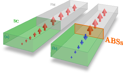
Figure 1: Schematics of the inverse proximity effect (IPE). The arrows represent the local magnetization vectors. The ABSs are absent and present at the interface in (a) and (b), respectively. When there are ABSs, the magnetization induced in the superconductor (SC) is opposite to that without ABS. The length scale of the IPE is characterized by the superconducting coherence length $\xi_{0}$.

In this paper, we theoretically study the IPE in F/USC junctions utilizing the quasiclassical Green’s function theory. We show that, when ABSs appear, the IPE induces a local magnetization with the opposite sign compared to that in the F/conventional-SC junction (see Fig. 1). Using a 1D model, we show that the direction of the induced magnetization is determined by two factors: existence of ABSs and the sign of the spin-mixing angle. We also show that spin-singlet and spin-triplet pairs near the interface show a correspondence when $T\sim T_{c}$. Odd-frequency spin-triplet $s$-wave pairs induced in a spin-triplet $p$-wave junction behave in the same way as spin-singlet $s$-wave pairs induced in an $s$-wave junction.

In a two-dimensional system, the sign of the spin-mixing angle in general depends on the momentum parallel to the interface, $k_{\parallel}$. When the magnetization in F is sufficiently small, the results are qualitatively the same as those in 1D system. In the case of a large magnetization in F, however, the $k_{\parallel}$ dependence of the spin-mixing angle cannot usually be ignored. As a result, in this latter case, the direction of the induced magnetization for superconductors with nodes at $k_{\parallel}=0$ is not simply determined by the two factors discussed in the 1D limit.

II Model and Formulation

In this paper, we consider two-dimensional ballistic superconducting junctions as shown in Fig. 1, where the interface is located at $x=0$. We discuss the magnetization induced at the interface of an F/SC junction, where F and SC stand for ferromagnet and superconductor.

Superconductivity in the ballistic limit can be described by the quasiclassical Eilenberger theory. The Green functions obey the Eilenberger equation:

$$i\boldsymbol{v}_{F}\cdot\boldsymbol{\nabla}\check{g}+\left[\check{H},~{}\check{g}\right]_{-}=0,$$ (1)

$$\check{g}=\left(\begin{array}[]{rr}\hat{g}&\hat{f}\\[2.84526pt] -\hat{\undertilde{f}}&-\hat{\undertilde{g}}\\ \end{array}\right),\hskip 11.38109pt\check{H}=\left(\begin{array}[]{cc}i\omega_{n}\hat{\sigma}_{0}&\hat{\eta}\\[2.84526pt] \hat{\undertilde{\eta}}&-i\omega_{n}\hat{\sigma}_{0}\end{array}\right),$$ (6)

where $\check{g}=\check{g}(x,\boldsymbol{k},i\omega_{n})$ is the Matsubara Green function and $\boldsymbol{v}_{F}$ is the Fermi velocity. In this paper, the accents $\check{\;}$ and $\hat{\;}$ denote matrices in particle-hole space and spin space, respectively. The identity matrices in particle-hole and spin space are denoted by $\check{\tau}_{0}$ and $\hat{\sigma}_{0}$. The Pauli matrices in particle-hole space and in spin space are $\check{\tau}_{j}$ and $\hat{\sigma}_{j}$ with $j\in\{1,2,3\}$, respectively. All of the functions satisfy the symmetry relation $\hat{K}(x,\boldsymbol{k},i\omega_{n})=[\hat{\undertilde{K}}(x,-\boldsymbol{k},i\omega_{n})]^{*}$, where the unit vector $\boldsymbol{k}$ represents the direction of the Fermi momentum. The effects of the F can be taken into account through boundary conditions.

The Eilenberger equation (1) must be supplemented by a normalization condition, $\check{g}^{2}=\check{1}$, which is nonlinear. It can be implemented explicitely by the so-called Riccati parametrization Schopohl and Maki (1995); Eschrig et al. (1999); Eschrig (2000, 2009); Eschrig et al. (2015). The Green function can be expressed in terms of the coherence function $\hat{\gamma}$ in the following way Eschrig (2009); Eschrig et al. (2015):

$$\check{g}=2\left(\begin{array}[]{rr}\hat{\mathcal{G}}&\hat{\mathcal{F}}\\[2.84526pt] -\hat{\undertilde{\mathcal{F}}}&-\hat{\undertilde{\mathcal{G}}}\\ \end{array}\right)-\check{\tau}_{3},$$ (9)

$$\hat{\mathcal{G}}=(1-\hat{\gamma}\hat{\undertilde{\gamma}})^{-1},\hskip 17.07164pt\hat{\mathcal{F}}=(1-\hat{\gamma}\hat{\undertilde{\gamma}})^{-1}\hat{\gamma},$$ (10)

$$\hat{\undertilde{\mathcal{G}}}=(1-\hat{\undertilde{\gamma}}\hat{\gamma})^{-1},\hskip 17.07164pt\hat{\undertilde{\mathcal{F}}}=(1-\hat{\undertilde{\gamma}}\hat{\gamma})^{-1}\hat{\undertilde{\gamma}},$$ (11)

where $\hat{\gamma}=\hat{\gamma}(x,\boldsymbol{k},i\omega_{n})$. The Riccati parametrization reduces the Eilenberger equation (1) into the Riccati-type differential equation Eschrig et al. (1999):

$$i\boldsymbol{v}_{F}\cdot\boldsymbol{\nabla}\hat{\gamma}+\hat{\xi}\hat{\gamma}-\hat{\gamma}\hat{\undertilde{\xi}}-\hat{{\eta}}+\hat{\gamma}\hat{\undertilde{\eta}}\hat{\gamma}=0.$$ (12)

This Riccati-Eilenberger equation can be simplified as

$$\boldsymbol{v}_{F}\cdot\boldsymbol{\nabla}\gamma+2\omega_{n}\gamma-\Delta_{\boldsymbol{k}}+\Delta_{\boldsymbol{k}}^{*}\gamma^{2}=0,$$ (13)

where we assume the superconductor has only one spin component [i.e., $\hat{\eta}=i\Delta_{\boldsymbol{k}}(i\hat{\sigma}_{\nu}\hat{\sigma}_{2})$ with $\nu\in\{0,1,2,3\}$] and the spin structure of the coherence function is parameterized as $\hat{\gamma}=\gamma(i\hat{\sigma}_{\nu}\hat{\sigma}_{2})$. In a homogeneous superconductor, the coherence function is given by

$$\bar{\gamma}(\boldsymbol{k},i\omega_{n})=\frac{\Delta_{\boldsymbol{k}}}{\omega_{n}+\sqrt{\omega_{n}^{2}+|\Delta_{\boldsymbol{k}}|^{2}}},$$ (14)

where the coherence function needs to satisfy the condition $\lim_{\omega_{n}\to\infty}\gamma=0$.

In USCs, the pair potential depends on the direction of the momentum. For isotropic Fermi surfaces, the momentum dependence of the pair potential is given by

$$\Delta_{\boldsymbol{k}}=\left\{\begin{array}[]{ll}\Delta_{0}&~{}\text{for $s$ wave,}\\ \Delta_{0}\cos\varphi&~{}\text{for $p_{x}$ wave,}\\ \Delta_{0}\sin\varphi&~{}\text{for $p_{y}$ wave,}\\ \Delta_{0}\cos(2\varphi)&~{}\text{for $d_{x^{2}-y^{2}}$ wave,}\\ \Delta_{0}\sin(2\varphi)&~{}\text{for $d_{xy}$ wave,}\\ \end{array}\right.$$ (20)

where $\varphi$ characterizes the direction of the Fermi momentum; $k_{x}=\cos\varphi$ and $k_{y}=\sin\varphi$. The temperature dependence of the pair potential is determined by the self-consistency condition for a homogeneous SC:

$$\Delta_{0}(T)=2N_{0}\lambda\frac{\pi}{\beta}\sum_{\omega_{n}>0}^{\omega_{c}}\int\frac{\Delta_{\varphi}\Lambda_{\varphi}}{\sqrt{\omega_{n}^{2}+\Delta_{\varphi}^{2}}}\frac{d\varphi}{2\pi}$$ (21)

where $N_{0}$ is the density of states (DOS) per spin at the Fermi level, $\beta=1/T$, $\omega_{c}$ is the BCS cutoff energy, and

$$\Lambda_{\varphi}=\left\{\begin{array}[]{ll}1&~{}\text{for $s$ wave,}\\ 2\cos\varphi&~{}\text{for $p_{x}$ wave,}\\ 2\sin\varphi&~{}\text{for $p_{y}$ wave,}\\ 2\cos(2\varphi)&~{}\text{for $d_{x^{2}-y^{2}}$ wave,}\\ 2\sin(2\varphi)&~{}\text{for $d_{xy}$ wave.}\\ \end{array}\right.$$ (27)

The coupling constant $\lambda$ is given by

$$\lambda=\frac{1}{N_{0}}\left[\mathrm{ln}\left(\frac{T}{T_{c}}\right)+\sum_{n=0}^{n_{c}}\frac{1}{n+1/2}\right]^{-1},$$ (28)

with $n_{c}=\omega_{c}/2\pi T$.

In this paper, the temperature dependence of the pair potential is taken into account, however the approximation of a spatially homogeneous pair potential is made.

Magnetic potentials can induce the local magnetization in the SC. The induced magnetization is defined as

$$M(x)=\mu_{B}(n_{\uparrow}-n_{\downarrow}),$$ (29)

$$n_{\alpha}(x)=\langle\Psi^{\dagger}_{\alpha}(x)\Psi_{\alpha}(x)\rangle$$ (30)

where $\mu_{B}$ is the effective Bohr magneton, $\alpha=$ $\uparrow$ or $\downarrow$ is the spin index, and $\Psi_{\alpha}$ ($\Psi^{\dagger}_{\alpha}$) is the annihilation (creation) operator of a particle with the spin $\alpha$. This local magnetization can be obtained from the diagonal parts of the quasiclassical Green’s function:

$$M(x) =\frac{\mu_{B}N_{0}\pi}{2i\beta}\sum_{\omega_{n}}\int\mathrm{Tr}\left[(\tau_{3}\otimes{\sigma}_{3})\hat{g}(x,\varphi,i\omega_{n})\right]\frac{d\varphi}{2\pi},$$

$$=2\pi\mu_{B}N_{0}T\sum_{n=0}^{n_{c}}\int\mathrm{Im}[g_{\uparrow}-g_{\downarrow}]\frac{d\varphi}{2\pi},$$ (31)

where we have used the symmetry of the Matsubara Green function $\hat{g}(x,\varphi,i\omega_{n})=-{\hat{g}}^{*}(x,\varphi,-i\omega_{n})$, and the abbreviation $\hat{g}=\mathrm{diag}[g_{+},g_{-}]$ with $g_{\pm}$ being the normal Green’s function for the up and down spin.

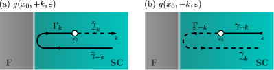
Figure 2: Quasiclassical path to obtain the Green’s function in $(+k,k_{y})$ and $(-k,k_{y})$ direction, respectively. The particle-like (hole-like) coherence function must be solved along the quasiclassical path in $+k$ ($-k$) direction, which are indicated by the solid and broken lines. The momentum parallel to the interface is conserved during the reflection. The overbar symbol $\bar{\cdot}$ denotes the bulk value of the coherence function.

II.1 Boundary condition

The boundary conditions for the coherence functions are given in Refs. Eschrig (2000, 2009); Eschrig et al. (2015). Hereafter, the outgoing (incoming) coherence functions are denoted by $\Gamma$ ($\gamma$) as introduced in Ref. Eschrig (2000). When the SC and F are semi-infinitely long in the $x$ direction, the boundary condition is simplified because $\gamma=0$ in the F. The boundary condition is given by

$$\hat{\Gamma}=\hat{r}\hat{\gamma}\hat{r}^{*},$$ (32)

where the reflection-coefficient matrix $\hat{r}$ is given by

$$\hat{r}=\left[\begin{array}[]{cc}r_{\uparrow}&\\ &r_{\downarrow}\end{array}\right]=\left[\begin{array}[]{cc}|r_{\uparrow}|e^{i(\phi+\theta_{\mathrm{SM}})}&\\ &|r_{\downarrow}|e^{i(\phi-\theta_{\mathrm{SM}})}\end{array}\right].$$ (37)

The angle $\theta_{\mathrm{SM}}$ is the so-called spin-mixing angle Tokuyasu et al. (1988) and $r_{\uparrow}$ and $r_{\downarrow}$ are the reflection coefficients for the up-spin and down-spin particles injected from the SC side. The reflection coefficients can be obtained by matching the wave functions:

$$r_{\alpha} =\frac{\hbar(v-v_{\alpha})-2iV}{\hbar(v+v_{\alpha})+2iV},$$ (38)

where we have assumed the potential barrier $V\delta(x)$ at the interface and $v=\hbar k/m$ ($v_{\alpha}=\hbar k_{\alpha}/m$) is the $x$ component of the Fermi velocity in the SC (F) side; $k=(2\mu_{S}-k_{y}^{2})^{1/2}$ and $k_{\uparrow(\downarrow)}=\{2m[\mu_{F}+(-)M_{0}]-k_{y}^{2}\}^{1/2}$ with $m$ being the effective mass of a quasiparticle. Note that we have made $\hbar$ explicit to avoid misunderstandings.

In a single-spin-component superconductor, the coherence amplitude in the bulk can be expressed as

$$\hat{\gamma}=\gamma(i\hat{\sigma}_{\nu}\hat{\sigma}_{2}),\hskip 22.76219pt\undertilde{\hat{\gamma}}=\undertilde{\gamma}(i\hat{\sigma}_{\nu}\hat{\sigma}_{2})^{\dagger}.$$ (39)

In the present case (i.e., magnetic potentials are parallel to the spin quantization axis), the reflection coefficients are diagonal in spin space (i.e., $\hat{r}=\mathrm{diag}[r_{\uparrow},r_{\downarrow}]$). Therefore, the outgoing coherence functions (32) are given by

$$\hat{\Gamma}=\left(\begin{array}[]{rr}&\Gamma_{\uparrow}\\ s_{\nu}\Gamma_{\downarrow}&\\ \end{array}\right)=\left(\begin{array}[]{rr}&r_{\uparrow}\gamma r^{*}_{\downarrow}\\ s_{\nu}r_{\downarrow}\gamma r^{*}_{\uparrow}&\\ \end{array}\right),$$ (44)

for the opposite-spin pairing ($\nu=0$ or $3$), where $s_{\nu}=1$ ($-1$) for the spin-triplet (singlet) pairing. The boundary conditions obtained here are consistent with those derived using the so-called evolution operators Ashida et al. (1989); Nagato et al. (1993); Tanuma et al. (2001); Hirai et al. (2003).

To obtain the coherence amplitude, we need to consider the group velocity of the quasiparticle and quasihole properly. The quasiclassical paths to obtain $\check{g}(x_{0},k,k_{y},\varepsilon)$ and $\check{g}(x_{0},-k,k_{y},\varepsilon)$ are shown in Figs. 2(a) and 2(b), where the solid and broken lines represent the path for the particle-like and hole-like coherence amplitudes and the direction of the arrows indicate the direction of the Fermi momentum. Since the quasiparticle (quasihole) propagates in the same (opposite) directions as $\boldsymbol{k}$, $\hat{\gamma}$ and $\undertilde{\hat{\gamma}}$ should be solved in $\boldsymbol{k}$ and $-\boldsymbol{k}$ direction respectively.

The Green’s function can be obtained from the coherence functions [see Eq. (9)]. Using the boundary condition, the diagonal part of the Green’s functions at the interface are given in terms of the coherence functions:

$$\hat{g}_{+k}=(1-\hat{\Gamma}\hat{\undertilde{\gamma}})^{-1}(1+\hat{\Gamma}\hat{\undertilde{\gamma}}),$$ (45)

$$\hat{g}_{-k}=(1-\hat{\gamma}\hat{\undertilde{\Gamma}})^{-1}(1+\hat{\gamma}\hat{\undertilde{\Gamma}}),$$ (46)

where $\hat{g}_{\pm k}=\hat{g}(x=0^{+},\pm k,k_{y},i\omega_{n})$. The spin-reduced Green’s functions at the interface are

$${g}_{\alpha,{+k}}=\frac{1+\Gamma_{\alpha}{\undertilde{\gamma}}}{1-\Gamma_{\alpha}{\undertilde{\gamma}}},\hskip 5.69054pt{g}_{\alpha,{-k}}=\frac{1+{\gamma}\undertilde{\Gamma}_{\alpha^{\prime}}}{1-{\gamma}\undertilde{\Gamma}_{\alpha^{\prime}}},$$ (47)

where $\alpha^{\prime}$ means the opposite spin of $\alpha$. The spin structure of the coherence functions are parameterized as $\hat{\Gamma}=\mathrm{diag}[\Gamma_{\uparrow},\Gamma_{\downarrow}](i\hat{\sigma}_{\nu}\hat{\sigma}_{2})$ and $\hat{\undertilde{\Gamma}}=\mathrm{diag}[\undertilde{\Gamma}_{\uparrow},\undertilde{\Gamma}_{\downarrow}](i\hat{\sigma}_{\nu}\hat{\sigma}_{2})^{\dagger}$. Assuming the spatially homogeneous pair potential, we can replace $\gamma$ in Eq. (47) by $\bar{\gamma}$, where the symbol $\bar{\;}$ means bulk values. This assumption changes the results only quantitatively but not qualitatively.

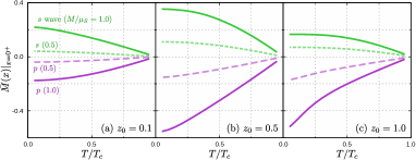
Figure 3: Temperature dependence of induced magnetization at the interface of a 1D FM/SC junction. The induced magnetization is normalized as $\bar{M}=M/2\pi\mu_{B}N_{0}T_{c}$. The magnetization of the F is set to $M_{0}=\mu_{F}$ or $0.5\mu_{F}$ with $\mu_{F}=\mu_{S}$. The spin-independent barrier potential is set to (a) $z_{0}=0.1$, (b) 0.5, and (c) 1.0, where $\theta_{\mathrm{SM}}<0$ for all of the sets of the parameters. The induced magnetization of the $s$-wave junctions is positive, whereas that of the $p$-wave junctions are negative. The pair potential depends on the temperature but is kept constant as function of the spatial coordinate $x$.

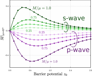
Figure 4: Induced magnetization at the interface of a 1D FM/SC junction. The magnetization $M|_{x=0^{+}}$ for $s$- and $p$-wave superconductors are respectively positive and negative regardless of the magnitude of $z_{0}$. The temperature is set to $T=0.2T_{c}$.

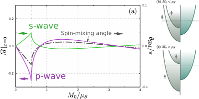
Figure 5: Induced magnetization and spin-mixing angle of a 1D F/SC junction as a function of $M_{0}$. The chemical potential in the F is set to $\mu_{F}=0.5\mu_{S}$, which means that the F is an FM (HM) when $M_{0}<0.5\mu_{S}$ ($M_{0}\geq 0.5\mu_{S}$). The schematic band structures of the FM/SC and HM/SC junctions are shown in (b) and (c), respectively. The sign of the magnetization is determined by $\mathrm{sgn}(M_{0})$ and the pairing symmetry. The temperature and the barrier potentials are set to $T=0.2T_{c}$ and $z_{0}=1$.

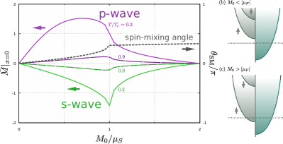
Figure 6: Induced magnetization and spin-mixing angle of a 1D F/SC junction with $\mu_{F}=-\mu_{S}$. The F is insulating for $M_{0}<\mu_{S}$ or a half-metallic for $M_{0}>\mu_{S}$. The induced magnetization for an $s$-wave junction is negative regardless of the temperature (i.e., $T=0.2T_{c}$ and $0.9T_{c}$), whereas that $p$-wave junctions are positive. The barrier potential is set to $z_{0}=0$. The $s$-wave results are consistent with those in Ref. Tokuyasu et al., 1988, where $\theta_{\mathrm{SM}}$ is defined with the opposite sign compared with our definition. The schematics of band structures of the FI/SC and HM/SC junctions are shown in (b) and (c), respectively.

III One-dimensional system

In order to understand the basics of the IPE. We start with one-dimensional (1D) systems. Such systems can be considered by setting $k_{y}=0$.

III.1 Ferromagnetic-metal junction

The temperature dependence of the induced magnetizations at the interface of the F/SC junction are shown in Fig. 3 where spin-singlet even-parity and spin-triplet odd-parity superconducting junctions are considered, which correspond to the $s$- and $p_{x}$-wave superconducting junctions in the 2D case respectively. The magnetization in the F is set to $M_{0}=\mu_{F}$ or $0.5\mu_{F}$ with $\mu_{F}=\mu_{S}$, the barrier potential $z_{0}=mV/k$ is set to (a) $z_{0}=0.1$, (b) $z_{0}=0.5$, and (c) $z_{0}=1.0$, and the pair potential is assumed spatially homogeneous but temperature dependent. In the even-parity case, the magnetization in the F induces the parallel magnetization in the SC as shown in Fig. 3. This behavior is consistent with that in the ballistic limit in Refs. Tollis et al. (2005); Bergeret et al. (2005b). In the odd-parity case, on the contrary, the induced magnetization is antiparallel to $M_{0}$. We have confirmed that no magnetization is induced when the $\boldsymbol{d}$-vector is perpendicular to the magnetization vector in the F.

The $z_{0}$ dependences of $M|_{x=0^{+}}$ are shown in Fig. 4. The induced magnetization is not a monotonic function of the barrier parameter $z_{0}$. When $z_{0}\to\infty$, the reflection coefficient (38) becomes spin-independent (i.e., $r_{\alpha}\to-1$). Therefore, $M_{x=0^{+}}$ vanishes in this limit. When $z_{0}=0$, the reflection coefficients in Eq. (38) are real as long as $k_{\alpha}$ is real (i.e., F is a ferromagnetic metal), which means that the reflected quasiparticles do not have an additional spin-dependent phase shift. As a result, no magnetization is induced in the SC .

The induced magnetization $M|_{x=0^{+}}$ and the spin-mixing angle $\theta_{\mathrm{SM}}$ as functions of $M_{0}$ are shown in Fig. 5(a) where $\mu_{F}=0.5\mu_{S}$, $z_{0}=1.0$, and $T=0.2T_{c}$. In this case, the F is a ferromagnetic metal (FM) for $0<M_{0}<\mu_{F}$ and a half-metal (HM) for $M_{0}>\mu_{F}$ as schematically illustrated in Figs. 5(b) and 5(c). As shown in Fig. 5(a), the sign of $M|_{x=0^{+}}$ for the $s$-wave junction is always opposite to $\mathrm{sgn}[\theta_{\mathrm{SM}}]$, whereas that for the $p$-wave junction always has the same sign. These results demonstrate that the sign of the induced magnetization is determined by the two factors: the pairing symmetry and the sign of the spin-mixing angle $\theta_{\mathrm{SM}}$.

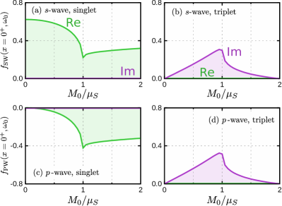
Figure 7: Pair amplitudes in a 1D F/$s$-wave junction. The $s$-wave spin-singlet, $s$-wave triplet, $p$ -wave singlet, and $p$ -wave triplet components are plotted in (a), (b), (c), and (d). When $M_{0}<\mu_{S}$ (i.e., FI regime), the magnetization is mainly generated by the product of the $s$-wave singlet and $s$-wave triplet pairs because the $s$-wave singlet is dominant [see Eq. (48)]. The temperature and the Matsubara frequency are set to $T=0.9T_{c}$ and $\omega_{n}=\omega_{0}$.

III.2 Ferromagnetic-insulator junction

The IPE occurs in ferromagnetic-insulator(FI)/SC junctions as well. The $M_{0}$ dependence of $M|_{x=0^{+}}$ is shown in Fig. 6(a). In order to model the FI, we set $\mu_{F}=-\mu_{S}$ where the FI-HM transition occurs at $M_{0}=|\mu_{F}|$ as schematically shown in Figs. 6(b) and 6(c). Figure 6(a) shows that $M|_{x=0^{+}}$ in the $s$-wave junction is antiparallel to $M_{0}$ in the F. This result is consistent with Ref. Tokuyasu et al., 1988 . For the $p$-wave case, on the other hand, the induced magnetization is parallel to $M_{0}$. We can conclude that the IPE induces the local magnetization with the opposite sign compared with an $s$-wave junction.

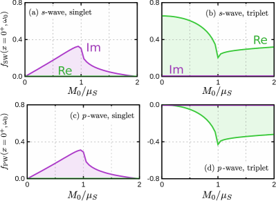
Figure 8: Pair amplitudes in a 1D F/$p$ -wave junction. The results are plotted in the same manner as in Fig. 7. The main contribution comes from the $s$-wave pairs even in the $p$ -wave spin-triplet superconducting junction.

At low temperature, $|M|$ in $M_{0}<\mu_{F}$ for the $p$-wave junction is greatly larger than that for the $s$-wave case. Similar low-temperature anomalies of the magnetic response have been reported so farAsano et al. (2011); Yokoyama et al. (2011); Suzuki and Asano (2014, 2015); Asano and Sasaki (2015); Higashitani et al. (2013); Suzuki and Asano (2014, 2016); Higashitani (2014a). These anomalies are explained by the emergence of the zero-energy ABSs. In superconducting junctions, ABSs appear because of the interference between the quasiparticle propagating into an interface and reflected one. Therefore, the effects of ABSs become larger as increasing reflection probability $|R|$ Kashiwaya and Tanaka (2000). In other words, the anomalous IPE becomes more prominent in an FI/SC junction than that in FM/SC and HM/SC junctions.

The amplitude of $M|_{x=0^{+}}$ changes suddenly at $M_{0}=|\mu_{F}|$ in accordance with the FI-HM transition. After the FI-HM transition, the induced magnetization decreases with increasing $M_{0}$ and vanishes at $M_{0}=2|\mu_{F}|$ regardless of the pairing symmetry. When $\mu_{F}\pm M_{0}=\mu_{S}$, the dispersion relation of either band in the F becomes identical to that in the SC, with the consequence that the reflection probability for the corresponding spin becomes zero. In this case, both $\Gamma_{\uparrow}$ and $\Gamma_{\downarrow}$ are zero [see Eq. (44)], which means the IPE does not occur.

The induced magnetization can be expressed in terms of the pair amplitude (i.e., anomalous Green’s function) when $T\sim T_{c}$ (see Appendix A for the details) Higashitani et al. (2013); Higashitani (2014b). In the 1D limit, in particular, the magnetization is give by

$$M\approx 4\pi\mu_{B}N_{0}T\sum_{\omega_{n}>0}m_{0,3},$$ (48)

$$m_{\nu,\nu^{\prime}}=\mathrm{Im}\big{[}f_{\nu,\mathrm{SW}}f^{*}_{\nu^{\prime},\mathrm{SW}}+f_{\nu,\mathrm{PW}}f^{*}_{\nu^{\prime},\mathrm{PW}}\big{]},$$ (49)

where SW and PW stand for the $s$-wave and $p$-wave pairings respectively. The spin indices $\nu=0$ and 3 represent the spin-singlet and spin-triplet pairs respectively. Note that $f_{0,PW}$ and $f_{3,SW}$ should be odd-functions of $\omega_{n}$ to satisfy the Pauli rule Eschrig et al. (2003); Eschrig and Löfwander (2008); Eschrig et al. (2007). Equation (48) means that the magnetization is given by the product of the spin-singlet and spin-triplet pairs.

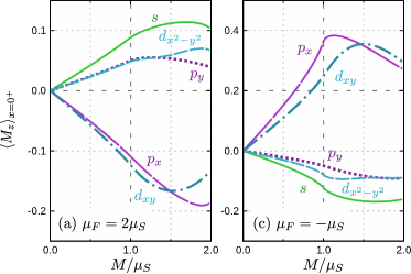
Figure 9: Induced magnetization of a 2D F/SC junction. The chemical potential is set to (a) $\mu_{F}=2\mu_{S}$ and (b) $\mu_{F}=-\mu_{S}$. When the ABSs are present, the induced magnetizations have the opposite sign to those without ABSs. The temperature and the barrier potentials are set to $T=0.2T_{c}$ and $z_{0}=1$.

The pair amplitudes at the interface of the $s$-wave junction are shown in Fig. 7, where $T=0.9T_{c}$ and $\omega=\omega_{0}=\pi T$. The spin-singlet $s$-wave, spin-triplet $s$-wave, spin-singlet $p$-wave, and spin-triplet $p$-wave pair amplitudes are shown in Figs. 7(a), 7(b), 7(c), and 7(d). In the FI region (i.e., $M_{0}<\mu_{F}$) of an $s$-wave junction, the conventional spin-singlet $s$-wave pairs are dominant and the other pair amplitudes are relatively small. The magnetization in this case is mainly generated by the spin-singlet and spin-triplet $s$-wave Cooper pairs (i.e., $f_{0,\mathrm{SW}}f^{*}_{3,\mathrm{SW}}\ll f_{0,\mathrm{PW}}f^{*}_{3,\mathrm{PW}}$ when $M_{0}\ll\mu_{F}$).

In the $p$-wave case, on the other hand, the spin-triplet $s$-wave pair amplitude is dominant for $M_{0}<\mu_{F}$ as shown in Fig. 8. In addition, the spin-triplet $s$-wave pair amplitudes have almost the same $M_{0}$ dependences for the spin-singlet $s$-wave pair amplitude as shown in Figs. 7(a) and 8(b). Comparing Figs. 7 and 8, similar correspondences between spin-singlet and spin-triplet pairs are confirmed. In Eq. (48), such a singlet-triplet conversion results in the sign change of the magnetization (i.e., $m_{0,3}=-m_{3,0}$). Namely, the $s$-wave pairs in the $p$-wave junction generate almost the same amplitude of the magnetization compared with the one in the $s$-wave junction. The direction, however, is opposite compared with that in the $s$-wave junction. In the Cooper pair picture, the spin structure of the dominant Cooper pair determines the direction of the induced magnetization.

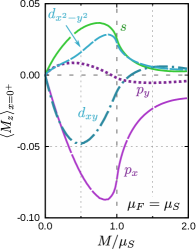
Figure 10: Induced magnetization of a 2D F/S junction with $\mu_{F}=\mu_{S}$. The results are plotted in the same manner in Fig. 9. When $M_{0}$ is sufficiently large, the induced magnetizations for an $s$-wave and $p_{y}$-wave junctions are opposite even though no ABS appears in both of the junctions.

IV Two-dimensional system

Most realistic superconducting junctions are two-dimensional or three-dimensional. In 2D systems, local quantities should be obtained via a $k_{y}$ integration, where $k_{y}$ is the momentum parallel to the interface (see Eq. (II)). In particuar, the induced magnetization generated by the IPE is obtained via $k_{y}$ integration where the partial magnetization depends on $k_{y}$ via the transport coefficients and the pair potential.

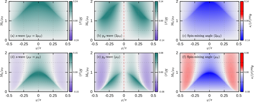
Figure 11: Angle-resolved magnetization and spin-mixing angle of F/SC junctions. The chemical potential in the F is set to $\mu_{F}=2\mu_{S}$ in (a)-(c), whereas $\mu_{F}=\mu_{S}$ in (d)-(f). The order parameter is assumed spin-singlet $s$-wave in (a) and (d), and spin-triplet $p$-wave in (b) and (e). When $\mu_{F}=\mu_{S}$ and $M_{0}\neq 0$, the sign change of $\theta_{\mathrm{SM}}$ occurs around $k_{y}\sim\pm k_{F}$. In (e), when $M_{0}>\mu_{F}$, the positive contribution to $M$ is smaller than the negative one due to the nodes of the $p_{y}$-wave gap at $\varphi=0$. In (a), (b), (d), and (e), the partial magnetizations are normalized to $\bar{M}(\varphi)=M(\varphi)/2\pi\mu_{B}N_{0}T_{c}$ and the magnetization in F is changed from $M_{0}=0.8$ to $2.0$ by $0.2$. The temperature and the barrier potentials are set to $T=0.2T_{c}$ and $z_{0}=0$.

The induced magnetizations in the 2D junctions are shown in Fig. 9, where the chemical potential in the F is set to (a) $\mu_{F}=2\mu_{S}$ and (b) $\mu_{F}=-\mu_{S}$. When $\mu_{F}=2\mu_{S}$, $\mathrm{sgn}(M)$ is determined by whether the ABSs are present or not. The anomalous IPE occurs when the ABSs are present at the interface (i.e., $p_{x}$- and $d_{xy}$-wave junctions). When $M_{0}<\mu_{F}$, all of the channels are regarded as FM/SC junctions which results in the parallel (antiparallel) magnetization in the SC without (with) ABSs as discussed in the 1D limit [see Fig. 5]. The direction of the induced magnetization does not change even in the $M_{0}>\mu_{S}$ region.

When $\mu_{F}=-\mu_{S}$, $\mathrm{sgn}(M)$ for each superconducting junction is inverted compared with Fig. 9(a). In the $M<\mu_{F}$ region, all of the channels are regarded as an FI/SC junction where the induced magnetization in the absence (presence) of ABSs is negative as discussed in the 1D limit. When $M_{0}>\mu_{F}$, even though the channels around $k_{y}=0$ change to HM/SC junctions, the sign of $\theta_{\mathrm{SM}}$ remains unchanged. Therefore, the total amplitude of the magnetization also remains unchanged.

When $M_{0}\gg\mu_{F}$ and $\mu_{F}=\mu_{S}$, the sign change of $\theta_{\mathrm{SM}}$ can not be ignored. The $M_{0}$ dependence of $M|_{x=0^{+}}$ for $\mu_{F}=\mu_{S}$ are shown in Fig. 10. In the $p_{y}$- and $d_{xy}$-wave case (i.e., SCs with gap nodes on the Fermi surface at $k_{y}=0$), the direction of the induced magnetization changes around $M_{0}=\mu_{F}$ as shown in Fig. 10. On the other hand, the signs of $M|_{x=0^{+}}$ for the $s$-, $p_{x}$-, and $d_{x^{2}-y^{2}}$-wave superconducting junction (i.e., SCs without gap does at $k_{y}=0$) are unchanged.

To understand the sign change of the induced magnetization, we evaluated the angle-resolved magnetization $M(\varphi)$ with $k_{y}=\sin\varphi$. The results for $s$- and $p_{y}$-wave junctions with $\mu_{F}=2\mu_{S}$ are shown in Figs. 11(a) and 11(b). In this case, $M(\varphi)$ are positive for both of the junctions because the sign of $\theta_{\mathrm{SM}}$ is always positive as shown in Fig. 11(c). Note that $M(\varphi)|_{\varphi=0}=0$ in the $p_{y}$-wave junction because of the nodes on the superconducting gap shown by the broken red line in Fig. 11(b).

The results with $\mu_{F}=\mu_{S}$ are shown in Figs. 11(d), 11(e), and 11(f). The spin-mixing angle can be negative when $M_{0}\neq 0$ as shown in Fig. 11(f) Eschrig (2018). In the $s$-wave junction with $M_{0}\neq 0$, the positive contribution (shown in green) around $\varphi=0$ is larger than the negative ones (shown in purple) around $|\varphi|=\pi/2$. The total magnetization, therefore, is always positive even for $\mu_{F}=\mu_{S}$ as shown in Fig. 10. In the $p_{y}$-wave junction, on the other hand, the positive contribution is smaller than in the $s$-wave case because of the nodes. As a result, the direction of the total magnetization can change around $M_{0}=\mu_{F}$ (Fig. 10).

V Discussions

The anomalous IPE presented in this paper can be observed by ferromagnetic resonance (FMR) measurements Mühge et al. (1998); Garifullin et al. (2002), by nuclear magnetic resonance (NMR) measurements Salikhov et al. (2009), and by polar Kerr effect measurements Xia et al. (2009). In these experiments the conventional IPE has been observed. Replacing the conventional SC by an USC such as a high-$T_{c}$ cuprate, it would possible to confirm experimentally the anomalous IPE.

In this paper, we assume that the pair potential depends only on the temperature but not on the coordinate. This assumption, however, changes the results only quantitatively but not qualitatively. Our main conclusion about the direction of the induced magnetization would remain unchanged even if we employ the spatial-dependent self-consistent pair potential.

VI Conclusion

We have theoretically studied the IPE in F/USC junctions utilizing the quasiclassical Green function theory. We have shown that the direction of the induced magnetization is determined by two factors: by whether the ABS exists and by the sign of the spin-mixing angle $\theta_{\mathrm{SM}}$. Namely, in the 1D limit, the induced magnetizations for the $p_{x}$-wave SC is always opposite to that for the $s$-wave SC.

In the 2D model, the spin-mixing angle $\theta_{\mathrm{SM}}$ depends on the momentum parallel to the interface $k_{y}$. The results for 2D F/SC junctions are qualitatively the same as those in the 1D limit when the magnetization in the F ($M_{0}$) is smaller than the chemical potential of the F ($\mu_{F}$). When $M_{0}\gg\mu_{F}$, the sign of the induced magnetization is not simply determined by the ABSs because the sign changes of $\theta_{\mathrm{SM}}$ around $k_{y}\sim\pm k_{F}$ are not negligible in this parameter range.

In addition, analyzing the pair amplitudes in 1D models, we have pointed out a correspondence at $T\sim T_{c}$ between the spin-singlet pairs in an $s$-wave junction and the spin-triplet pairs in a $p$-wave junction. The odd-frequency spin-triplet $s$-wave pairs induced in the spin-triplet $p$-wave junction have qualitatively the same $M_{0}$ dependence as that for the spin-singlet $s$-wave pairs induced in the $s$-wave junction. Reflecting this correspondence, the amplitudes of the induced magnetizations in the $s$- and $p$-wave junctions are qualitatively the same. Their directions, however, are opposite to each other, where the direction of the magnetization is determined by the relative phase between the spin-singlet and spin-singlet pair functions.

Appendix A Symmetry of Cooper pairs and induced magnetization

When there is a spin-dependent potential, subdominant pairing component must be induced because of the symmetry breaking. Near the interface of an F/SC junction, the anomalous Green functions are expressed as a superposition of the spin-triplet and singlet pairs:

$$\hat{g}=\mathrm{diag}[g_{\uparrow},g_{\downarrow}],\hskip 17.07164pt \hat{f}=f_{0}i\hat{\sigma}_{2}+f_{3}\hat{\sigma}_{1},$$ (50)

$$\undertilde{\hat{f}}=\undertilde{f}_{0}(-i\hat{\sigma}_{2})+\undertilde{f}_{3}\hat{\sigma}_{1},$$ (51)

where we consider a spin-dependent potential parallel to the spin quantization axis. From the normalization condition (i.e., $\hat{g}^{2}-\hat{f}\undertilde{\hat{f}}=\hat{\sigma}_{0}$), we have the explicit forms for $g_{\uparrow}$ and $g_{\downarrow}$: $g_{\uparrow(\downarrow)}^{2}=[1+f_{0}\undertilde{f}_{0}+f_{3}\undertilde{f}_{3}]+(-)[f_{0}\undertilde{f}_{3}+f_{3}\undertilde{f}_{0}]$. When $T\sim T_{c}$, the pair amplitude is sufficiently small. Accordingly, the approximated Green’s function and the local magnetization are given by the following expressions:

$$g_{\uparrow(\downarrow)}=1+\frac{1}{2}\left\{[f_{0}\undertilde{f}_{0}+f_{3}\undertilde{f}_{3}]+(-)[f_{0}\undertilde{f}_{3}+f_{3}\undertilde{f}_{0}]\right\}$$

$$M(x)\approx 2\pi\mu_{B}N_{0}T\sum_{\omega_{n}>0}\int_{-\pi}^{\pi}\mathrm{Im}\big{[}f_{0}\undertilde{f}_{3}+f_{3}\undertilde{f}_{0}\big{]}\,\frac{d\varphi}{2\pi}.$$ (52)

In a 2D system, the anomalous Green’s function can be expanded in a Fourier series:

$$f_{\nu}=\frac{C_{\nu,0}}{\sqrt{2\pi}}+\frac{1}{\sqrt{\pi}}\sum_{l>0}\left[C_{\nu,l}\cos(l\varphi)+S_{\nu,l}\sin(l\varphi)\right],$$ (53)

where $C_{\nu,n}$ are $S_{\nu,n}$ are coefficients that represent each pairing amplitude (e.g., $C_{\nu=0,0}$, $C_{3,1}$, and $S_{3,2}$ correspond to the $s$-wave spin-singlet, $p_{x}$-wave spin-triplet, and $d_{xy}$-wave spin-triplet pairs). Note that the spin-singlet odd-parity and spin-triplet even-parity components should be odd functions with respect to the Matsubara frequency. In other words, they represent the odd-frequency pair amplitudes. Using $\undertilde{f}(x,\varphi,i\omega_{n})=f^{*}(x,\varphi+\pi,i\omega_{n})$ and the orthogonality of the trigonometric functions, we can obtain

$$M(x)=4\pi\mu_{B}N_{0}T\sum_{\omega_{n}>0}\mathrm{Im}\big{[}C_{0,0}C^{*}_{3,0}+\sum_{l>0}(-1)^{l}\left(C_{0,l}C^{*}_{3,l}+S_{0,l}S^{*}_{3,l}\right)\big{]}.$$ (54)

In the 1D limit, in particular, the magnetization is given by

$$M=4\pi\mu_{B}N_{0}T\sum_{\omega_{n}>0}\mathrm{Im}\big{[}f_{0,\mathrm{SW}}f^{*}_{3,\mathrm{SW}}+f_{0,\mathrm{PW}}f^{*}_{3,\mathrm{PW}}\big{]},$$ (55)

where SW and PW stand for $s$- and $p$-wave pairings (i.e., even-parity and odd-parity pairing in the 1D limit). The magnetization is generated by the product of the spin-singlet and spin-triplet pairs.

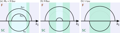
Figure 12: Evolution of the Fermi surfaces. The chemical potentials are set to $\mu_{F}=\mu_{S}$. The magnetization is set to (a) $M_{0}=0.5\mu_{F}$, (b) $0.9\mu_{F}$, and (c) $1.1\mu_{F}$. There are two Fermi surfaces in the F in the light-blue region, whereas only one Fermi surface exists in the green region. The outer light-purple region is irrelevant to the IPE.

Appendix B Spin-mixing angle and Fermi surfaces

The sign of the spin-mixing angle $\theta_{\mathrm{SM}}$ is not simply determined by whether the F is an FM or HM Eschrig (2018). We show the evolution of the Fermi surfaces in Fig. 12, where the chemical potentials are set to $\mu_{F}=\mu_{S}$. The magnetization is set to (a) $M_{0}=0.5\mu_{F}$, (b) $0.9\mu_{F}$, and (c) $1.1\mu_{F}$. Increasing $M_{0}$, the spin bands split in the F. As a result, there is only one Fermi surface for the channels with $k_{\parallel}$ as shown in the green region in Fig. 12. When $M_{0}>\mu_{F}$, the Fermi surface for the down-spin band vanishes. Comparing Figs. 12 and 11(f), we see that $\mathrm{sgn}[\theta_{\mathrm{SM}}]$ is not in an obvious way related to the band structure in the F.

In junctions of a ferromagnet and a normal metal, the spin-dependent potentials in the magnet give rise to a phase delay of the wave function for the reflected quasiparticle Eschrig (2018). The quasiparticle injected from the normal metal penetrates into the ferromagnet even when the process is classically forbidden. The quasiparticle is reflected after experiencing the spin-dependent potential, which results in an additional phase. Therefore, the spin-mixing angle is not only determined by the electronic structure in the ferromagnet but by how the quasiparticle experiences the magnetic potentials at the interface.

References

- Bardeen et al. (1957) J. Bardeen, L. N. Cooper, and J. R. Schrieffer, Phys. Rev. 108, 1175 (1957).
- Buchholtz and Zwicknagl (1981) L. J. Buchholtz and G. Zwicknagl, Phys. Rev. B 23, 5788 (1981).
- Hara and Nagai (1986) J. Hara and K. Nagai, Progress of Theoretical Physics 76, 1237 (1986).
- Hu (1994) C.-R. Hu, Phys. Rev. Lett. 72, 1526 (1994).
- Tanaka and Kashiwaya (1995) Y. Tanaka and S. Kashiwaya, Phys. Rev. Lett. 74, 3451 (1995).
- Kashiwaya and Tanaka (2000) S. Kashiwaya and Y. Tanaka, Reports on Progress in Physics 63, 1641 (2000).
- Löfwander et al. (2001) T. Löfwander, V. S. Shumeiko, and G. Wendin, Superconductor Science and Technology 14, R53 (2001).
- Tanaka and Kashiwaya (1997) Y. Tanaka and S. Kashiwaya, Phys. Rev. B 56, 892 (1997).
- Asano (2001) Y. Asano, Phys. Rev. B 64, 014511 (2001).
- Eschrig et al. (2003) M. Eschrig, J. Kopu, J. C. Cuevas, and G. Schön, Phys. Rev. Lett. 90, 137003 (2003).
- Tanaka and Kashiwaya (2004) Y. Tanaka and S. Kashiwaya, Phys. Rev. B 70, 012507 (2004).
- Asano et al. (2004) Y. Asano, Y. Tanaka, and S. Kashiwaya, Phys. Rev. B 69, 134501 (2004).
- Kwon et al. (2004) H.-J. Kwon, K. Sengupta, and V. M. Yakovenko, The European Physical Journal B-Condensed Matter and Complex Systems 37, 349 (2004).
- Krawiec et al. (2004) M. Krawiec, B. L. Györffy, and J. F. Annett, Phys. Rev. B 70, 134519 (2004).
- Kopu et al. (2004) J. Kopu, M. Eschrig, J. C. Cuevas, and M. Fogelström, Phys. Rev. B 69, 094501 (2004).
- Eschrig et al. (2004) M. Eschrig, J. Kopu, A. Konstandin, J. C. Cuevas, M. Fogelström, and G. Schön, Adv. in Solid State Phys. , 533 (2004).
- Buzdin (2005) A. I. Buzdin, Rev. Mod. Phys. 77, 935 (2005).
- Bergeret et al. (2005a) F. S. Bergeret, A. F. Volkov, and K. B. Efetov, Rev. Mod. Phys. 77, 1321 (2005a).
- Asano et al. (2006) Y. Asano, Y. Tanaka, T. Yokoyama, and S. Kashiwaya, Phys. Rev. B 74, 064507 (2006).
- Asano et al. (2007a) Y. Asano, Y. Tanaka, A. A. Golubov, and S. Kashiwaya, Phys. Rev. Lett. 99, 067005 (2007a).
- Keizer et al. (2006) R. Keizer, S. Goennenwein, T. Klapwijk, G. Miao, G. Xiao, and A. Gupta, Nature 439, 825 (2006).
- Eschrig and Löfwander (2008) M. Eschrig and T. Löfwander, Nature Physics 4, 138 (2008).
- Asano et al. (2007b) Y. Asano, Y. Tanaka, and A. A. Golubov, Phys. Rev. Lett. 98, 107002 (2007b).
- Braude and Nazarov (2007) V. Braude and Y. V. Nazarov, Phys. Rev. Lett. 98, 077003 (2007).
- Houzet and Buzdin (2007) M. Houzet and A. I. Buzdin, Phys. Rev. B 76, 060504 (2007).
- Galaktionov et al. (2008) A. V. Galaktionov, M. S. Kalenkov, and A. D. Zaikin, Phys. Rev. B 77, 094520 (2008).
- Zhao and Sauls (2008) E. Zhao and J. A. Sauls, Phys. Rev. B 78, 174511 (2008).
- Kalenkov and Zaikin (2010) M. S. Kalenkov and A. D. Zaikin, Phys. Rev. B 82, 024522 (2010).
- Löfwander et al. (2010) T. Löfwander, R. Grein, and M. Eschrig, Phys. Rev. Lett. 105, 207001 (2010).
- Metalidis et al. (2010) G. Metalidis, M. Eschrig, R. Grein, and G. Schön, Phys. Rev. B 82, 180503 (2010).
- Eschrig (2011) M. Eschrig, Phys. Today 64, 43 (2011).
- Tanaka et al. (2012) Y. Tanaka, M. Sato, and N. Nagaosa, J. Phys. Soc. Jpn. 81, 011013 (2012).
- Machon et al. (2013) P. Machon, M. Eschrig, and W. Belzig, Phys. Rev. Lett. 110, 047002 (2013).
- Machon et al. (2014) P. Machon, M. Eschrig, and W. Belzig, New Journal of Physics 16, 073002 (2014).
- Ozaeta et al. (2014) A. Ozaeta, P. Virtanen, F. S. Bergeret, and T. T. Heikkilä, Phys. Rev. Lett. 112, 057001 (2014).
- Di Bernardo et al. (2015a) A. Di Bernardo, S. Diesch, Y. Gu, J. Linder, G. Divitini, C. Ducati, E. Scheer, M. G. Blamire, and J. W. Robinson, Nat. Commun. 6, 1 (2015a).
- Linder and Robinson (2015) J. Linder and J. W. Robinson, Nat. Phys. 11, 307 (2015).
- Eschrig (2015) M. Eschrig, Reports on Progress in Physics 78, 104501 (2015).
- Eschrig (2018) M. Eschrig, Phil. Trans. R. Soc. A 376, 20150149 (2018).
- Suzuki et al. (2020) S.-I. Suzuki, M. Sato, and Y. Tanaka, Phys. Rev. B 101, 054505 (2020).
- Higashitani (1997) S. Higashitani, J. Phys. Soc. Jpn. 66, 2556 (1997).
- Tanaka et al. (2005) Y. Tanaka, Y. Asano, A. A. Golubov, and S. Kashiwaya, Phys. Rev. B 72, 140503 (2005).
- Asano et al. (2011) Y. Asano, A. A. Golubov, Y. V. Fominov, and Y. Tanaka, Phys. Rev. Lett. 107, 087001 (2011).
- Yokoyama et al. (2011) T. Yokoyama, Y. Tanaka, and N. Nagaosa, Phys. Rev. Lett. 106, 246601 (2011).
- Suzuki and Asano (2014) S.-I. Suzuki and Y. Asano, Phys. Rev. B 89, 184508 (2014).
- Di Bernardo et al. (2015b) A. Di Bernardo, Z. Salman, X. L. Wang, M. Amado, M. Egilmez, M. G. Flokstra, A. Suter, S. L. Lee, J. H. Zhao, T. Prokscha, E. Morenzoni, M. G. Blamire, J. Linder, and J. W. A. Robinson, Phys. Rev. X 5, 041021 (2015b).
- Suzuki and Asano (2015) S.-I. Suzuki and Y. Asano, Phys. Rev. B 91, 214510 (2015).
- Asano and Sasaki (2015) Y. Asano and A. Sasaki, Phys. Rev. B 92, 224508 (2015).
- Suzuki and Asano (2016) S.-I. Suzuki and Y. Asano, Phys. Rev. B 94, 155302 (2016).
- Lee et al. (2017) S.-P. Lee, R. M. Lutchyn, and J. Maciejko, Phys. Rev. B 95, 184506 (2017).
- Krieger et al. (2020) J. A. Krieger, A. Pertsova, S. R. Giblin, M. Döbeli, T. Prokscha, C. W. Schneider, A. Suter, T. Hesjedal, A. V. Balatsky, and Z. Salman, Phys. Rev. Lett. 125, 026802 (2020).
- Higashitani et al. (2013) S. Higashitani, H. Takeuchi, S. Matsuo, Y. Nagato, and K. Nagai, Phys. Rev. Lett. 110, 175301 (2013).
- Higashitani (2014a) S. Higashitani, Phys. Rev. B 89, 184505 (2014a).
- Deutscher and De Gennes (1969) G. Deutscher and P. De Gennes, Marcel Dekker, New York 2, 1005 (1969).
- Volkov et al. (1993) A. Volkov, A. Zaitsev, and T. Klapwijk, Physica C: Superconductivity 210, 21 (1993).
- Golubov and Kupriyanov (1988) A. Golubov and M. Y. Kupriyanov, J. Low Temp. Phys. 70, 83 (1988).
- Golubov and Kupriyanov (1989) A. Golubov and M. Y. Kupriyanov, Zh. Èksp. Teor. Fiz. 96,1420 [Sov. Phys. JETP 69, 805 (1989)] (1989).
- Golubov et al. (1997) A. A. Golubov, F. K. Wilhelm, and A. D. Zaikin, Phys. Rev. B 55, 1123 (1997).
- Suzuki et al. (2019) S.-I. Suzuki, A. A. Golubov, Y. Asano, and Y. Tanaka, Phys. Rev. B 100, 024511 (2019).
- Tanaka et al. (2007) Y. Tanaka, Y. Tanuma, and A. A. Golubov, Phys. Rev. B 76, 054522 (2007).
- Berezinskii (1974) V. L. Berezinskii, Zh. Eksp. Teor. Fiz. 20, 628 (1974) [JETP Lett.20, 287 (1974)] (1974).
- Balatsky and Abrahams (1992) A. Balatsky and E. Abrahams, Phys. Rev. B 45, 13125 (1992).
- Fominov et al. (2015) Y. V. Fominov, Y. Tanaka, Y. Asano, and M. Eschrig, Phys. Rev. B 91, 144514 (2015).
- Tokuyasu et al. (1988) T. Tokuyasu, J. A. Sauls, and D. Rainer, Phys. Rev. B 38, 8823 (1988).
- Bergeret et al. (2004) F. S. Bergeret, A. F. Volkov, and K. B. Efetov, Phys. Rev. B 69, 174504 (2004).
- Tollis et al. (2005) S. Tollis, M. Daumens, and A. Buzdin, Phys. Rev. B 71, 024510 (2005).
- Bergeret et al. (2005b) F. S. Bergeret, A. L. Yeyati, and A. Martín-Rodero, Phys. Rev. B 72, 064524 (2005b).
- Salikhov et al. (2009) R. I. Salikhov, I. A. Garifullin, N. N. Garif’yanov, L. R. Tagirov, K. Theis-Bröhl, K. Westerholt, and H. Zabel, Phys. Rev. Lett. 102, 087003 (2009).
- Xia et al. (2009) J. Xia, V. Shelukhin, M. Karpovski, A. Kapitulnik, and A. Palevski, Phys. Rev. Lett. 102, 087004 (2009).
- Grein et al. (2013) R. Grein, T. Löfwander, and M. Eschrig, Phys. Rev. B 88, 054502 (2013).
- Yagovtsev et al. (2020) V. Yagovtsev, N. Pugach, and M. Eschrig, Superconductor Science and Technology (2020).
- Mühge et al. (1998) T. Mühge, Y. V. Goryunov, K. Theis-Bröhl, K. Westerholt, H. Zabel, and I. Garifullin, Applied Magnetic Resonance 14, 567 (1998).
- Garifullin et al. (2002) I. Garifullin, D. Tikhonov, N. Garifyanov, M. Fattakhov, K. Theis-Bröhl, K. Westerholt, and H. Zabel, Appl. Magn. Reson. 22, 439 (2002).
- Schopohl and Maki (1995) N. Schopohl and K. Maki, Phys. Rev. B 52, 490 (1995).
- Eschrig et al. (1999) M. Eschrig, J. A. Sauls, and D. Rainer, Phys. Rev. B 60, 10447 (1999).
- Eschrig (2000) M. Eschrig, Phys. Rev. B 61, 9061 (2000).
- Eschrig (2009) M. Eschrig, Phys. Rev. B 80, 134511 (2009).
- Eschrig et al. (2015) M. Eschrig, A. Cottet, W. Belzig, and J. Linder, New J. Phys. 17, 083037 (2015).
- Ashida et al. (1989) M. Ashida, S. Aoyama, J. Hara, and K. Nagai, Phys. Rev. B 40, 8673 (1989).
- Nagato et al. (1993) Y. Nagato, K. Nagai, and J. Hara, J. Low Temp. Phys. 93, 33 (1993).
- Tanuma et al. (2001) Y. Tanuma, Y. Tanaka, and S. Kashiwaya, Phys. Rev. B 64, 214519 (2001).
- Hirai et al. (2003) T. Hirai, Y. Tanaka, N. Yoshida, Y. Asano, J. Inoue, and S. Kashiwaya, Phys. Rev. B 67, 174501 (2003).
- Note (1) Note that we have confirmed for all set of and .
- Note (2) The spin-mixing angle in Ref. \rev@citealpnumTokuyasu_PRB_88 is defined with an extra minus sign compared with ours.
- Higashitani (2014b) S. Higashitani, J. Phys. Soc. Jpn. 83, 075002 (2014b).
- Eschrig et al. (2007) M. Eschrig, T. Löfwander, T. Champel, J. Cuevas, J. Kopu, and G. Schön, J. Low Temp. Phys. 147, 457 (2007).