Action potential propagation and block in a model of atrial tissue with myocyte-fibroblast coupling

Abstract

The electrical coupling between myocytes and fibroblasts and the spacial distribution of fibroblasts within myocardial tissues are significant factors in triggering and sustaining cardiac arrhythmias but their roles are poorly understood. This article describes both direct numerical simulations and an asymptotic theory of propagation and block of electrical excitation in a model of atrial tissue with myocyte-fibroblast coupling. In particular, three idealised fibroblast distributions are introduced: uniform distribution, fibroblast barrier and myocyte strait, all believed to be constituent blocks of realistic fibroblast distributions. Primary action potential biomarkers including conduction velocity, peak potential and triangulation index are estimated from direct simulations in all cases. Propagation block is found to occur at certain critical values of the parameters defining each idealised fibroblast distribution and these critical values are accurately determined. An asymptotic theory proposed earlier is extended and applied to the case of a uniform fibroblast distribution. Biomarker values are obtained from hybrid analytical-numerical solutions of coupled fast-time and slow-time periodic boundary value problems and compare well to direct numerical simulations. The boundary of absolute refractoriness is determined solely by the fast-time problem and is found to depend on the values of the myocyte potential and on the slow inactivation variable of the sodium current ahead of the propagating pulse. In turn, these quantities are estimated from the slow-time problem using a regular perturbation expansion to find the steady state of the coupled myocyte-fibroblast kinetics. The asymptotic theory gives a simple analytical expression that captures with remarkable accuracy the block of propagation in the presence of fibroblasts. Electrophysiology, Myocyte-Fibroblast Coupling, Refractoriness, Asymptotic Approximation

1 Introduction

The cardiac rhythm is controlled by electrical signals. The disruption of cardiac electrical signalling results in abnormalities causing the heart to beat too slowly, too quickly, or irregularly. These abnormalities are known as arrhythmias and their effects may range from minor discomfort to sudden death (Huikuri et al.,, 2001; Qu & Weiss,, 2015). In addition to cardiac myocytes, the cells that actively generate and transmit electrical signals in the heart, other non-myocyte cells play a significant role in the development of arrhythmias and electrical dysfunction. The most abundant type of non-myocyte cells in the heart are the cardiac fibroblasts – a heterogeneous group of cells whose phenotype and main functions vary in response to the pathological conditions of the heart (Brown et al.,, 2005). In normal myocardium the fibroblasts are primarily responsible for homeostatic maintenance of extracellular collagenous matrix. In injured myocardium the fibroblasts, activated by cytokines, transition into a distinct myofibroblast phenotype, proliferate and act as the key cells in the wound healing response, in particular they secrete a collagen-based polymer matrix to support myocytes. Several cardiac diseases such as myocardial infarction (MI) and dilated cardiomyopathy are thus associated with an increased density of fibroblasts. The arrhythmogenic action of fibroblasts is believed to occur via two main mechanisms (a) production of excess collagen that decouples cardiomyocytes and causes convoluted conduction paths resulting in substrates prone to electrical dysfunction (de Jong et al.,, 2011) and (b) direct electrical interaction with myocytes via gap junction channels (Chilton et al.,, 2007; Louault et al.,, 2008). The latter mechanism is somewhat less studied in the literature and it is the focus of this article.

Mathematical modelling plays an important role in understanding the arrhythmogenic electrical interactions of cardiomyocytes and fibroblasts which are otherwise difficult to separate and study in vivo. Two types of models have been proposed for the electrical properties of the single fibroblast – passive and active. The active models (Jacquemet & Henriquez,, 2007; MacCannell et al.,, 2007) incorporate the discovery that cardiac fibroblasts express voltage-gated K+ currents (Chilton et al.,, 2005), while the passive models (Nayak et al.,, 2013) regard fibroblasts as inert electrical loads. While most models describe ventricular fibroblasts, atrial versions (Burstein et al.,, 2008) and myofibroblast phenotype versions (Chatelier et al.,, 2012; Koivumäki et al.,, 2014) are also available. For upscaling to tissue level either a cell-insertion approach or a cell-attachment approach is commonly adopted (Xie et al., 2009a, ). Single-cell and tissue models have been used to study a variety of effects of myocyte-fibroblast electrical coupling including changes in action potential morphology (MacCannell et al.,, 2007), excitability and conduction velocity (Miragoli et al., 2006a, ; Xie et al., 2009a, ), spontaneous self-excitation (Miragoli et al.,, 2007; Greisas & Zlochiver,, 2012), propensity to early after-depolarisation and cardiac alternans (Nguyen et al.,, 2011), and vulnerability to reentry (Majumder et al.,, 2012; Gomez et al., 2014b, ; Gomez et al., 2014a, ). Modelling tends to veer towards using realistic patient-specific 3D computational models (McDowell et al.,, 2011), an approach that, while clinically most relevant, due to its complexity is not well-suited to disentangle and explain causal effects and possible mechanisms of arrhythmogenesis.

Conduction disturbances, spatially non-uniform conduction and conduction block are thought to be key elements in the initiation and maintenance of one of the two main types of arrhythmias, the reentrant arrhythmias, of which tachycardia, atrial and ventricular fibrillation are prominent examples (Antzelevitch & Burashnikov,, 2011; Qu & Weiss,, 2015). Reentry around anatomic or functional obstacles is determined by both conduction velocity and refractoriness. A reentrant arrhythmia occurs when the length of a circuit exceeds the wavelength of the circulating excitation given by the product of its conduction velocity and its refractory period. Thus, to understand reentrant arrhythmogenesis in post-MI fibrous substrates we aim to model conduction velocity and refractoriness in tissues composed of coupled myocytes and fibroblasts. While conduction velocity or equivalently activation times are routinely measured experimentally e.g. (Dietrichs et al.,, 2020; Erem et al.,, 2011) and computed from direct numerical simulations e.g. (Xie et al., 2009a, ) there are few attempts for rigorous theoretical analysis, see discussions in (Tyson & Keener,, 1988; Meron,, 1992). These attempts have been based almost universally on conceptual models of FitzHugh-Nagumo type (FitzHugh,, 1961; Nagumo et al.,, 1962) that are incapable of reproducing slow repolarisation, slow sub-threshold response, fast accommodation and other features of cardiac excitability crucial for understanding and controlling arrhythmogenesis (Biktashev,, 2002; Biktashev et al.,, 2008). To address these deficiencies we developed earlier an asymptotic procedure for analysis of detailed cardiac ion current models (Biktasheva et al.,, 2006; Biktashev et al.,, 2008). The key step consists of embedding asymptotically small parameters in the detailed models considered based on (a) a formal analysis of the time-scales of evolution of dynamic variables, (b) the largeness of the maximal value of the sodium current $I_{\mathrm{Na}}$ compared to other currents and (c) the quasi-stationary permeability of the $I_{\mathrm{Na}}$ ionic gates in certain potential ranges. The asymptotic embedding procedure reveals that, unlike systems of FitzHugh-Nagumo type, cardiac models have non-Tikhonov asymptotic structure (Tikhonov,, 1952; Pontryagin,, 1957) including qualitatively new features of topological nature (Simitev & Biktashev,, 2011). Asymptotic model reduction based on such embedding is capable of reproducing essential spatiotemporal phenomena of cardiac electrical excitation as demonstrated in (Simitev & Biktashev,, 2011) using several different cardiac ionic models. In (Simitev & Biktashev,, 2006), a simplified version of the procedure was used to achieve numerically accurate prediction of the front propagation velocity (within 16%) and its profile (within 0.7 mV) for a realistic model of human atrial tissue (Courtemanche et al.,, 1998). The asymptotic reduction was sufficiently simple to allow the derivation of an analytical condition for propagation block in a re-entrant wave which was in an excellent agreement with results of direct numerical simulations of the realistic atrial ionic model.

In this work, we wish to adapt and extend the analysis of (Simitev & Biktashev,, 2006) in order to study conduction velocity and conduction block in tissues composed of coupled myocytes and fibroblasts. In particular, we wish to demonstrate that the asymptotic theory discussed above will also apply with little modification in the case of myocyte-fibroblast coupling. However, we expect that conduction velocity will depend on the ratio of fibroblasts to myocytes in the tissue via changes that coupling elicits to the resting potential and to the action potential shape (Jacquemet & Henriquez,, 2008; Xie et al., 2009b, ). Further to this, we wish to use the asymptotic theory to explain the critical ratio of fibroblasts to myocytes at which a homogeneous and isotropic patch of fibrous tissue will block conduction and act as an anatomical obstacle. In reality, fibrous tissue is, of course, highly inhomogeneous and anisotropic (Nguyen et al.,, 2014; Yamamura et al.,, 2018). Arrhythmogenic risk predominantly arises in the border zone of a fibrotic post myocardial infarction zone where the boundaries between necrotic and morphologically viable myocardium are nonlinear and characterized by irregular edges wherein islands or bundles of myocytes are interdigitated by scar tissue (Arbustini et al.,, 2018). While details of the scar morphology depend on a multitude of factors and very patient-specific, it seems possible to identify a small number of commonly occurring, simple fibrotic inhomogeneities and investigate their transmission capacity. We focus in particular, on two seemingly typical fibrotic inhomogeneities that we will refer to as “straits” and “barriers”. Straits can be described as channels collinear with the direction of electrical conduction that have small fibroblast-to-myocyte ratio and are bordered on both sides by regions with large fibroblast-to-myocyte ratio. Barriers can be described as strips perpendicular to the direction of conduction that have large fibroblast-to-myocyte ratio and separate regions of small fibroblast-to-myocyte ratio. We suggest that other more complicated fibroblast distributions seen in histology can be understood on the basis of these and other basic inhomogeneities.

The article is structured as follows. In Section 2, we formulate our mathematical model of fibrous atrial tissue including three particular versions of the monodomain equations used, the form of myocyte-fibroblast coupling current, parameter values, model kinetics and auxiliary conditions. We proceed to describe three idealised fibroblast distribution cases that we believe are constituent blocks of realistic fibroblast distributions. We also briefly summarize the Strang operator-splitting method used for numerical solution. In Section 3, we present results from direct numerical simulations of the three idealised fibroblast distributions. In particular, we report simulated values of the primary action potential biomarkers routinely measured in experiments on electrical excitation in myocardial tissues e.g. by optical mapping. We also measure the critical values of the parameters defining the three idealised fibroblast distributions at which action potential propagation failure occurs. In Section 4, we extend and apply the asymptotic theory of Biktashev et al., (2008); Simitev & Biktashev, (2011) to the case of uniform fibroblast distribution. Appropriate fast-time and slow-time systems are derived and coupled asymptotically. Solutions are of these asymptotic problems are obtained, notably analytical expressions for the resting steady state of the coupled myocyte-fibroblast kinetics using a regular perturbation expansion. We conclude with a discussion of results and questions for further work in Section 5.

2 Mathematical models and numerical methods

2.1 Mathematical model of fibrous atrial tissue

To model the propagation of electrical excitation in two-dimensional fibrous atrial tissue we use the monodomain equations, see e.g. (Sundnes et al.,, 2006; Franzone et al.,, 2014), in the modified form,

$$\chi\left(C_{\text{m}}\frac{\partial V_{\text{m}}}{\partial t}+I_{\text{m}}(V_{\text{m}})+n(\mathbf{x})G_{\text{gap}}(V_{\text{m}}-V_{\text{f}})+I_{\text{stim}}(\mathbf{x},t)\right) =\nabla\cdot(\mathbf{\sigma}\nabla V_{\text{m}})\quad\text{in}\quad\Omega\times(0,\infty),$$ (2.1a)

$$C_{\text{f}}\frac{\partial V_{\text{f}}}{\partial t}+I_{\text{f}}(V_{\text{f}})+G_{\text{gap}}(V_{\text{f}}-V_{\text{m}}) =0\quad\text{in}\quad\Omega\times(0,\infty),$$ (2.1b)

$$\mathbf{k}\cdot\nabla V_{\text{m}} =0\quad\text{in}\quad\partial\Omega\times(0,\infty).$$ (2.1c)

The problem is posed in a rectangular region $\Omega=[0,L_{x}]\times[0,L_{y}]\subset\mathbb{R}^{2}$ of sizes $L_{x}$ and $L_{y}$ in the $x$- and the $y$-directions, respectively, with a unit normal $\mathbf{k}$ to its boundary $\partial\Omega$. Time is denoted by $t$, and the position vector is given by $\mathbf{x}=(x,y)$ in a Cartesian coordinate system shown in Fig. 1. Here, $V_{\text{m}}(\mathbf{x},t)$ and $V_{\text{f}}(\mathbf{x},t)$ denote myocyte and fibroblast transmembrane potentials and $C_{\text{m}}$ and $C_{\text{f}}$ are myocyte and fibroblast membrane capacitances, respectively. The constant $\chi$ denotes cell surface-to-volume ratio, and $\mathbf{\sigma}$ is a constant, second-order conductivity tensor, with an anisotropy ratio of approximately 15:2. The terms $I_{\text{m}}(V_{\text{m}})$ and $I_{\text{f}}(V_{\text{f}})$ represent the sum of voltage-dependent ionic currents across myocyte and fibroblast membranes as defined in the realistic human atrial cell model of Courtemanche et al., (1998) and in the active fibroblast model of Morgan et al., (2016), respectively. The stimulus current $I_{\text{stim}}(\mathbf{x},t)$ has a profile of a periodic train of rectangular impulses with amplitude $I_{s}$, extent $x_{s}$, duration $t_{s}$, and period (basic cycle length) $B$,

$$I_{\text{stim}}(x,y,t)=I_{s}\,H(x_{s}-x)\left[1+\operatorname{sgn}\left(\sin\frac{\pi t}{B}\right)\operatorname{sgn}\left(\sin\frac{\pi(t-B-2t_{s})}{B}\right)\right]$$ (2.2)

where $H(x)$ is the Heaviside step function. Default parameter values are listed in Table 1 and used throughout unless specified otherwise. Resting values of the dynamical variables are used as initial conditions as discussed further in Section 3.

Symbol	Parameter	Value	Unit	Source Ref.
$L_{x}$	domain length	50	mm	–
$L_{y}$	domain width	10	mm	–
$C_{\text{m}}$	myocyte capacitance	100	pFmm-2	(Courtemanche et al.,, 1998)
$C_{\text{f}}$	fibroblast capacitance	6.3	pFmm-2	(MacCannell et al.,, 2007)
$G_{\text{gap}}$	intercell conductance	0.5	nS	(Morgan et al.,, 2016)
$\chi$	surface-to-volume ratio	140	mm-1	(Niederer et al.,, 2011)
$\sigma(\mathbf{x})$	conductivity tensor	$\begin{pmatrix}0.1334&0\\ 0&0.0176\end{pmatrix}$	Sm-1	(Niederer et al.,, 2011)
$I_{s}$	stimulus current amplitude	-2000	pA	(Courtemanche et al.,, 1998)
$x_{s}$	stimulus extent	1	mm	(Courtemanche et al.,, 1998)
$t_{s}$	stimulus duration	2	ms	(Courtemanche et al.,, 1998)
$B$	basic cycle length	variable	ms	–
$I_{\text{m}}(V_{\text{m}})$	myocyte current kinetics	variable	pA	(Courtemanche et al.,, 1998)
$I_{\text{f}}(V_{\text{f}})$	fibroblast current kinetics	variable	pA	(Morgan et al.,, 2016)

Table 1: Default values of model parameters and kinetics used in equations (2.1).

The realistic human atrial cell model of Courtemanche et al., (1998) used here includes all major transmembrane currents responsible for AP generation such as $I_{\text{Na}}$, $I_{\text{Kur}}$, $I_{\text{to}}$, $I_{\text{Kr}}$, $I_{\text{Ks}}$, $I_{\text{CaL}}$, $I_{\text{K1}}$, $I_{\text{NaK}}$, and $I_{NCX}$. The model also incorporates a description of intracellular Ca²⁺ handling that accounts for the uptake and release currents $J_{\text{up}}$ (SERCA) and $J_{\text{rel}}$ (RyR) of the sarcoplasmic reticulum as well as K⁺, Na⁺ and Ca²⁺ homeostasis regulating intracellular ionic concentrations. We have chosen to use this model as it gives the opportunity to validate our numerical codes against data available in the literature, and to use asymptotic results already obtained in this case by Simitev & Biktashev, (2006). Constant values for the components of the conductivity tensor $\sigma$ are assumed in equation (2.1a) since we wish to focus the attention on the arrhythmogenic role of direct electrical interaction between myocytes and fibroblasts rather than on the better studied effects of excess collagen density in fibrotic regions.

In equations (2.1) a fixed number of identical fibroblasts, $n(x,y)$, are connected in parallel to each myocyte via an inter-cell conductance $G_{\text{gap}}$. This arrangement represents the so called “single-sided” fibroblast-myocyte connection proposed by Kohl & Camelliti, (2007) where fibroblasts electrically couple to one (or more) myocytes that are themselves electrically well-connected to each other while there are no fibroblast-fibroblast connections. A similar arrangement was referred to as “fibroblast-attachment” in (Xie et al., 2009a, ).

2.2 Idealised fibroblast distributions

The function $n(x,y)$ can be used to prescribe realistic non-uniform fibroblast distributions of variable severity such as reported in (Nguyen et al.,, 2014; Yamamura et al.,, 2018; Arbustini et al.,, 2018). However, here we restrict the attention to three simple cases illustrated in Fig. 1(b) that are perhaps characteristic of the distributions arising in border zones between intact myocardium and mature scars, an example shown in Fig. 1(a). In particular, we consider the following profiles of $n(x,y)$.

1. Uniform fibroblast distribution prescribed by

   $$n(x,y)=N,$$ (2.3a)

   where $$N N=0 N>0 N$$ is a constant over the entire domain. This case is schematically illustrated in boxes C1a and C1b of Fig. 1(b) with describing intact myocardium with no fibroblasts and indicating fibroblasts attached to each myocyte, respectively.

2. “Fibroblast barrier” distribution prescribed by

   $$n(x,y)=N\,H\big{(}(L_{x}/2+\Delta x)-x\big{)}H\big{(}x-(L_{x}/2-\Delta x)\big{)},$$ (2.3b)

   where intact myocardium with no attached fibroblasts is separated by a rectangular region of constant width $\Delta x$ extending uniformly in the $y$-direction where $N$ fibroblasts are attached to each myocyte. This case is a simplification of the situation schematically illustrated in box C2 of Fig. 1(b).

3. “Myocyte strait” distribution prescribed by

   $$n(x,y)=N\,\big{(}H\big{(}(L_{y}/2-\Delta y)-y\big{)}+H\big{(}y-(L_{y}/2+\Delta y)\big{)}\big{)},$$ (2.3c)

   where intact myocardium, in the shape of a rectangular region of constant width $\Delta y$, extends uniformly in the $x$-direction and channelled by fibrotic regions on both sides where $N$ fibroblasts are attached to each myocyte. This case is schematically illustrated in box C3 of Fig. 1(b).

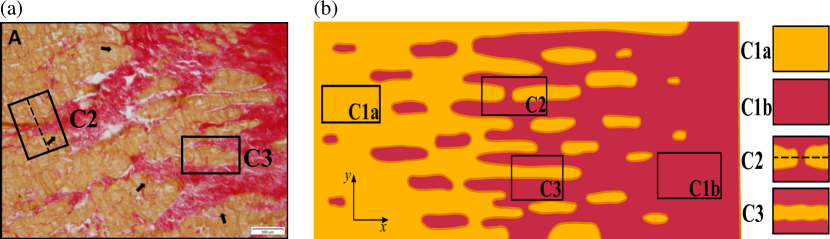
Figure 1: (a) An example of fibrosis in a specimen of cardiac tissue with collagen stained in red and intact myocardium shown in yellow from Yamamura et al., (2018). (b) A schematic illustration of a border zone between intact myocardium (to the left) and fibrosis (to the right) where the darker shaded areas indicate increased fibroblast density. The rectangular regions denoted in (b) correspond to the specific forms of the fibroblast distribution function $n(x,y)$ considered, see text.

2.3 Numerical methods

In order to obtain numerical solutions of the fibroblast-myocyte monodomain equations we write system (2.1) in the form

$$\frac{\partial}{\partial t}\begin{bmatrix}V_{\text{m}}\\ V_{\text{f}}\end{bmatrix}=\operatorname{\mathcal{A}}\begin{bmatrix}V_{\text{m}}\\ V_{\text{f}}\end{bmatrix}+\operatorname{\mathcal{B}}\begin{bmatrix}V_{\text{m}}\\ V_{\text{f}}\end{bmatrix},$$ (2.4)

where $\operatorname{\mathcal{A}}$ and $\operatorname{\mathcal{B}}$ are nonlinear differential operators defined by

$$\operatorname{\mathcal{A}}\begin{bmatrix}V_{\text{m}}\\ V_{\text{f}}\end{bmatrix}\equiv-\operatorname{diag}\left(\frac{1}{C_{\text{m}}}\Big{(}I_{\text{m}}(V_{\text{m}})+n(\mathbf{x})\,G_{\text{gap}}(V_{\text{m}}-V_{\text{f}})+I_{\text{stim}}\Big{)},\;\frac{1}{C_{\text{f}}}\Big{(}I_{\text{f}}(V_{\text{f}})+G_{\text{gap}}(V_{\text{f}}-V_{\text{m}})\Big{)}\right),$$ (2.5a)

$$\operatorname{\mathcal{B}}\begin{bmatrix}V_{\text{m}}\\ V_{\text{f}}\end{bmatrix}\equiv\operatorname{diag}\left(\frac{1}{\chi C_{\text{m}}}\nabla\cdot(\mathbf{\sigma}\cdot\nabla V_{\text{m}}),\;\;0\right).$$ (2.5b)

Following Qu & Garfinkel, (1999), we then apply the classical operator splitting method of Strang, (1968) and numerically approximate the solution vector $[V_{\text{m}},V_{\text{f}}]^{T}_{k\Delta t}$ after $k$ time steps of length $\Delta t$ by the following second-order accurate in time, formal $\theta$-scheme with $\theta=1/2$

$$\begin{bmatrix}V_{\text{m}}\\ V_{\text{f}}\end{bmatrix}_{k\Delta t}=\bigg{(}e^{(1-\theta)\Delta t\operatorname{\mathcal{A}}}\;\;e^{\Delta t\operatorname{\mathcal{B}}}\;\;e^{\theta\Delta t\operatorname{\mathcal{A}}}\bigg{)}^{k}\begin{bmatrix}V_{\text{m}}\\ V_{\text{f}}\end{bmatrix}_{0}+O(\Delta t^{2}),\qquad\qquad k=0,1,\dots,$$ (2.6)

where $[V_{\text{m}},V_{\text{f}}]^{T}_{0}$ are specified initial conditions and $e^{X}\equiv\sum_{m=0}^{\infty}X^{m}/m!$ is an operator exponential.

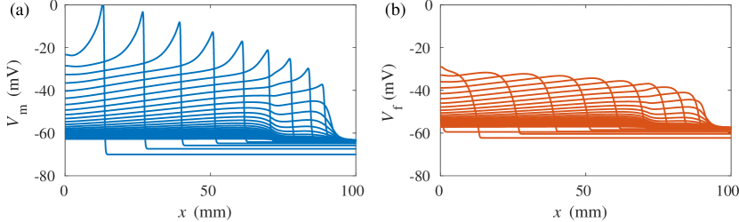
Figure 2: Myocyte and fibroblast action potentials $V_{\text{m}}$ in (a) and $V_{\text{f}}$ in (b), respectively, propagating in the $x$-direction in tissue with uniform fibroblast distribution (2.3a). Propagation is illustrated by potential profiles plotted at 25 ms time intervals apart. Fibroblast count $N$=12, other parameter values are listed in Table 1 and $B\to\infty$.

The practical implementation of the scheme consists of splitting the monodomain problem (2.1) into three Cauchy problems coupled to each other via their initial conditions as formally represented by the three nested operator exponentials in equation (2.6). The problems represented by the exponentials of $\operatorname{\mathcal{A}}$ consist of a spatially-decoupled nonlinear system of stiff ordinary differential equations and are solved using an fourth-order implicit Runge-Kutta method. The problem represented by the exponential of $\operatorname{\mathcal{B}}$ is a linear diffusion equation which is spatially discretised using a low-order finite element scheme and implemented in the open-source parallel C++ finite element library libMesh (Kirk et al.,, 2006) following the implementation reported by Rossi & Griffith, (2017). The numerical simulation code has been validated in Mortensen et al., (2018) against the benchmark paper of Niederer et al., (2011). Due to the stiffness of the ionic current system, a high-resolution spatial mesh with typical size 0.1 mm and a time step of 0.005 ms is required to resolve the upstrokes of propagating action potentials.

3 Direct numerical simulations of propagation in fibrous tissue

In this section, we present results from direct numerical simulations of equations (2.1) for the three choices of fibroblast distribution (2.3) introduced in Section 2. In each of these cases we provide numerical values of selected biomarkers typically used to characterise propagation in experimental measurements. In particular, we report values of conduction velocity, peak potential, peak intracellular calcium transient, APD${}_{\text{90}}$ duration and triangulation index as functions of the number of fibroblasts per myocyte. Action potential excitation and conduction are inhibited as fibroblast count increases, and we proceed to estimate the critical parameters of the fibroblast distributions (2.3) at which propagation block occurs.

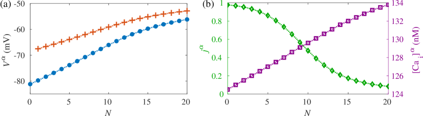
Figure 3: (a) Resting values of the myocyte potential $V^{\alpha}_{\text{m}}$ (blue full circles) and of the fibroblast potential $V^{\alpha}_{\text{f}}$, (red crosses), (b) resting values of the myocyte gating variable $j^{\alpha}$ (green diamonds, left ordinate scale) and of the internal myocyte calcium concentration (violet squares, right ordinate scale) all as functions of the fibroblast count $N$ in the case of uniform fibroblast distribution (2.3a). Other parameter values are listed in Table 1 and $I_{s}=0$.

3.1 The case of uniform fibroblast distribution (C1)

The basic effects of myocyte-fibroblast electrical coupling on conduction are best understood in the simple case C1 of uniform fibroblast distribution (2.3a) which we proceed to discuss here. Fig. 2 shows a numerical thought experiment that illustrates visually many of the phenomena analysed further in the text and their underlying mechanisms. Here, a tissue model with $N=12$ fibroblasts coupled to each myocyte is considered. Myocyte and fibroblast variables are set initially to the resting values of uncoupled cells as defined in Courtemanche et al., (1998) and Morgan et al., (2016), respectively. A stimulation by a current injection with a single impulse (i.e. $B\to\infty$ in (2.2)) is performed. The myocyte and fibroblast transmembrane potentials assume typical action potential profiles as shown in Fig. 2. As the signals propagate in the $x$-direction and in time, their peak values $V_{\text{m}}^{\omega}$ and $V_{\text{f}}^{\omega}$ decrease while the pre-front potentials $V_{\text{m}}^{\alpha}$ and $V_{\text{f}}^{\alpha}$ increase. The overall shapes of the action potentials change and most notably the steep profile of the myocyte potential, $V_{\text{m}}$ is eroded and assumes a much more diffusive profile than initially. This coincides with a slowdown of conduction until eventually decay of the action potentials occurs. Since conduction velocity and action potential features depend on the state of the medium ahead of the front this behaviour in our experiment can be explained by the process of relaxation of pre-front values of the myocyte and fibroblast potentials, gating variables, and ionic concentrations to their resting states. This relaxation occurs simultaneously with the propagation of the AP into the tissue. The resting state of the coupled myocyte-fibroblast system is different from the resting states of the uncoupled myocytes and fibroblast cells and Fig. 3 shows the equilibrium values $V^{\alpha}_{\text{m}}$ and $V^{\alpha}_{\text{f}}$ of myocyte and fibroblast potentials and, as examples, also of the slow inactivation gating variable of the myocyte sodium current $j^{\alpha}$ and of the resting calcium concentration, $\text{[Ca}_{\text{i}}]^{\alpha}$, all as functions of the number of coupled fibroblasts $N$. For each value of $N$, the resting values are computed by suppressing stimulation and leaving the tissues to relax for 1000 ms at which moment the equilibrium values are recorded. The pre-front potentials $V^{\alpha}_{\text{m}}$ and $V^{\alpha}_{\text{f}}$ as well as the $\text{[Ca}_{\text{i}}]^{\alpha}$ increase monotonically while $j^{\alpha}$ decreases from their respective uncoupled values with the increase of the number of coupled fibroblasts $N$.

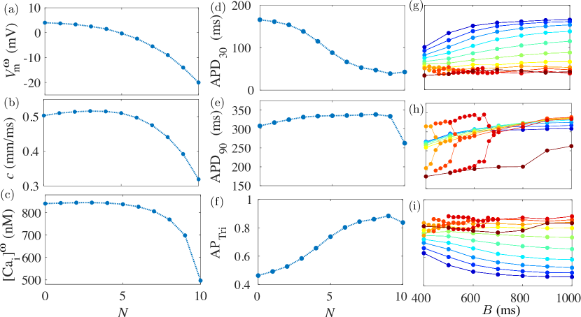
Figure 4: (a) Peak myocyte potential, $V_{\text{m}}^{\omega}$, (b) AP wave speed, $c$, (c) peak internal myocyte calcium concentration, (d) myocyte APD₃₀ (e) myocyte APD₉₀ and (f) normalised triangulation index, AP${}_{\text{Tri}}$, as functions of the number of coupled fibroblasts $N$ in the uniform case (2.3a) and for a single stimulus $B\to\infty$. (g) Myocyte APD₃₀ (h) myocyte APD₉₀ and (i) normalised triangulation index, AP${}_{\text{Tri}}$, as functions of basic cycle length $B$. In (h-i) the coloured lines represent different numbers of coupled fibroblasts, with dark blue corresponding to $N=0$ and dark red corresponding to and $N=10$, respectively, with the rest of the values on a heat map color scale.

Fig. 4 shows the dependences of other selected AP biomarkers commonly measured experimentally on the number of coupled fibroblasts $N$. The most significant result is the existence of a critical number of fibroblasts beyond which action potential propagation is inhibited and the tissue relaxes to equilibrium soon after stimulation. At the parameter values used in Fig. 4 this critical number is $N_{\text{crit}}=10$. At values of $N$ smaller than this critical value, normal action potentials are established and travel in the $x$-direction with constant wave speed, $c$, and fixed shape. These can be characterised with the value of their peak potential, $V^{\omega}$, the action potential duration, APD₉₀, defined as the time taken for the AP to return to 90% repolarisation after the initial depolarisation, and the normalised triangulation index,

$$\text{AP}_{\text{Tri}}=\frac{\text{APD}_{90}-\text{APD}_{30}}{\text{APD}_{90}}.$$

Wave speed values, $c$, exhibit non-monotonic behaviour with a slight increase in the interval $N\in[0,4]$ and decrease for larger values of $N$ until $N_{\text{crit}}$ is reached as shown in Fig. 4(b). This behaviour is similar to the “biphasic” behaviour reported by Miragoli et al., 2006b in experiments and by Xie et al., 2009a in simulations of a cell-attached model. This non-monotonicity was suggested to occur because wave speed first increases by the fibroblast bringing the membrane potential closer to the threshold for sodium current activation but then decreases as the increasing fibroblast density shift the cardiomyocyte membrane resting potential and sodium inactivation as discussed above. This will be subject to further theoretical modelling in Section 4 further below. With the increase of the number of coupled fibroblasts $N$, both the peak potential values $V^{\omega}$ (Fig. 4(a)) and the values of APD₃₀ (Fig. 4(d)) decrease, while the values of APD₃₀ (Fig. 4(e)) somewhat increase, before collapse at $N_{\text{crit}}=10$, giving rise to increasingly triangular AP profile as measured by APD${}_{\text{Tri}}$ (Fig. 4(f)). Another important quantity is the internal myocyte calcium concentration, $\text{[Ca}_{\text{i}}]$ which is directly linked the magnitude of myocyte contraction, and is used to couple electrophysiological models to models of sarcomere mechanics (Rice et al.,, 2008). The peak calcium concentration shown in Fig. 4(c) stays relatively constant until after $N=6$, after which it decreases. Without coupling the EP model to a model of contraction, it is clear that coupling a high number of fibroblasts will affect muscle contraction significantly.

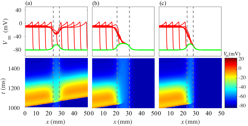
Figure 5: Examples of propagation and block of action potentials travelling in a direction perpendicular to a fibroblast barrier case C2 (2.3b) with (a) $N=15$ and $\Delta x=5$ mm, (b) $N=15$ and $\Delta x=10$ mm, and (c) $N=18$ with $\Delta x=5$ mm, respectively. The top row shows cross-sections in the $x$-direction of the myocyte transmembrane potentials at the middle of the simulation domains, $L_{y}/2$, and at time intervals of 10 ms after 1000 ms of initial relaxation, i.e. $V_{\text{m}}(x,y=L_{y}/2,t=1000+10k)$, $k=0,1,2\dots$ The resting profile at $t=1000$ ms is shown by a thick green line. The bottom row shows density map plots of $V_{\text{m}}$ as a function of the $x$-direction and time at $y=L_{y}/2$. The thin grey broken vertical lines show the location and the width $\Delta x$ of the fibroblast barriers in each case.

Usually, tissue is paced periodically in vivo as well as in vitro. To mimic this we investigated the effects that changing the basic cycle length $B$ (BCL) has on the action potential profile and its propagation. Simulations were performed for $N<N_{\text{crit}}$ for a physiological range of BCLs ranging from 300ms (200bpm) to 1000ms (60bpm). To allow the stimulated APs to adjust to the BCL a tissue of length 20mm was simulated for 6000ms, again leaving the tissue to relax in the initial 1000ms before the first stimulation. As the BCL was increased both the APD₃₀ shown in Fig. 4(g) and the APD₉₀ shown in Fig. 4(h) increase. However, when the fibroblast count $N$ reaches $N=7,8,9$, alternans occur for shorter BCL. At $N=10$ alternans do not appear, this is likely due to the value being too close to the threshold of excitation. The restitution curves end when the BCL becomes too short to successfully stimulate every AP. For the smaller values of $N$, the normalised triangulation index, AP${}_{\text{Tri}}$ shown in Fig. 4(i) increases weakly for small BCL, but for larger BCL the AP${}_{\text{Tri}}$ remains relatively constant. Action potential triangulation as an important pro-arrhythmic index (Hondeghem et al.,, 2001).

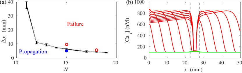
Figure 6: (a) The threshold curve separating the outcomes of propagation and block of action potential in the $(N-\Delta x)$ plane in the case of fibroblast barrier distribution (2.3b). The error bars show the nearest pair of grid points where simulations were run in order to construct the curve with the curve taken at midpoints. The markers show the locations of the three examples illustrated in Fig. 5 with full blue circles indicating successful propagation and empty red circles indicating block. (b) Cross-sections of calcium concentration transient $[\text{Ca}_{i}](x,y=L_{y}/2,t=1000+10k)$, $k=0,1,2\dots$ in the case $N=15$ and $\Delta x=5$mm plotted in style similar to the panels in the top row of Fig. 5 Thin grey broken vertical lines show the location and the width $\Delta x$ of the fibroblast barrier.

3.2 The case of “fibroblast barrier” distribution (C2)

We now consider the idealized “fibroblast barrier” example of a non-uniform fibroblast distribution defined by expression (2.3b). This case represents healthy myocardium characterised by small fibroblast density split in two by a fibrous region of high fibroblast density where $N$ fibroblasts are attached to each myocyte. The region has a rectangular shape of constant width $\Delta x$ extending uniformly in the $y$-direction. We expect that action potential propagation/failure in this case will depend on both the width $\Delta x$ and the fibroblast count $N$ – the two parameters needed to define this fibroblast distribution. To illustrate this we show in Fig. 5 three examples of action potentials propagating in the direction perpendicular to a fibroblast barrier. Similarly to the uniform case C1, the tissue is left to relax for 1000 ms before stimulation commences. Panels (a) and (b) of Fig. 5 show barrier distributions with identical fibroblast counts $N=15$ but different widths $\Delta x$ and illustrate that a wide barrier region can block the propagation of an incident action potential. Panels (a) and (c) of Fig. 5 show barrier distributions with identical widths $\Delta x=5$ mm but different fibroblast counts $N$ and illustrate that a large fibroblast count $N$ within the barrier can also block propagation, similarly to the uniform case of the preceding section. These examples suggest that there exist critical values of the fibroblast barrier distribution parameters $N$ and $\Delta x$ over which block occurs. The locus of these values forms a critical curve that serves as a threshold separating the outcomes of successful propagation and block in the $(N-\Delta x)$ parameter space and is shown in Fig. 6(a). The threshold curve plays a similar role and appears similar in shape to “strength-duration” curves, familiar from experimental electrophysiology, that serve to determine the threshold of electrical excitation as functions of the stimulus current amplitude and duration. We note that as the fibroblast count $N$ approaches 10 from above, $\Delta x$ increases asymptotically consistent with the behaviour of the uniform case C1 discussed in the preceding section.

The threshold behaviour described above is the essential feature of the fibroblast barrier case C2. Because the barrier is relatively thin its effect on the propagating action potential is only transient if it is not blocked. In the extensive healthy regions far from the fibroblast barrier action potential biomarkers behave in the same way as in the uniform case C1 described in relation to Fig. 4. For instance, Fig. 6(b) shows the calcium concentration profile propagating across a fibroblast barrier with $N=15$ and $\Delta x=5$ mm. While in the barrier region the calcium concentration is significantly less than in the “healthy” region, it quickly recovers on the exit of this relatively narrow strip.

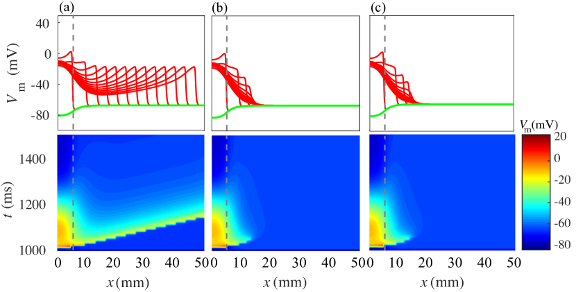
Figure 7: Examples of propagation and block of action potentials travelling down myocyte straits C3 (2.3c) with (a) $N=15$ and $\Delta y=0.6$ mm, (b) $N=15$ and $\Delta y=0.4$ mm, and (c) $N=18$ and $\Delta y=0.6$ mm, respectively. Thin grey broken vertical lines show the left end of the myocyte straits and other plot elements are as described in the caption of Fig. 5.

3.3 The case of “myocyte strait” distribution (C3)

Another simple idealised pattern that appears to be a constituent of realistic non-uniform fibrosis is that of a relatively thin strand of viable myocytes surrounded on both sides by fibrous tissue. This distribution is defined by expression (2.3c) and we will refer to it as a “myocyte strait” (C3). Similarly to the fibroblast barrier, a myocyte strait is determined by two free parameters – its width $\Delta y$ and the fibroblast count $N$ in the adjacent fibrous regions, and similarly, we expect that action potential propagation and failure depend on both. As an illustration, we show in Fig. 7 three examples of action potentials propagating $x$-direction through myocyte straits. For illustrative purposes, the fibroblast distribution used in these three cases differ from equation (2.3c) in that fibroblast-free regions at $x<5$ mm have been appended in front of the myocyte straits so that the effect of the action potentials entering the straits can be clearly seen. As in preceding cases discussed, the configuration is left to relax to resting state for 1000 ms, before action potentials are stimulated. Panel (a) of Fig. 7 shows an action potential propagating successfully through a strait of width $\Delta y=$0.6 mm with 15 fibroblasts coupled to each myocyte on either side of the strand. The corresponding propagation of the calcium transient in this case is shown in Fig. 8(b). Propagation block occurs when strait width is reduced as illustrated in Fig. 7(b) for $\Delta y=$0.4 mm and the same fibroblast count with $N=15$ as in panel (a). Propagation block also occurs when the fibroblast count in the flanking fibrotic regions is increased as demonstrated in Fig. 7(c) for a strand with $\Delta y=$0.6 mm, identical to that of panel (a) but with $N=18$. The critical threshold curve separating the regions where successful propagation and block occur in the $(N-\Delta y)$ parameter space is shown in Fig. 8(a). The threshold curve tends to $N=10$ from above as $\Delta y$ tends to 0 mm in agreement with the uniform case C1.

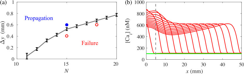
Figure 8: (a) The threshold curve separating the outcomes of propagation and block of action potential in the $(N-\Delta y$) plane in the case of myocyte strait distribution (2.3c). The circles represent the three examples shown in Fig. 7. (b) Cross-sections of calcium concentration transient $[\text{Ca}_{i}]$ propagating through a myocyte strait with $N=15$ and $\Delta y=5$ mm. Formatting conventions in both panels are identical to these used in Fig. 6.

Biomarkers of action potentials propagating down myocyte straits are plotted in Fig. 9. Each line in the plots connects values with the same strand width $\Delta y$ increasing from 0.1 mm to 0.9 mm, for a range of fibroblast counts $N\in[11,20]$ in the flanking fibrous regions. As $N$ increases the peak potential, $V^{\omega}$, the wave speed $c$ and the peak calcium concentration $[\text{Ca}_{i}]^{\omega}$ all decrease until the action potential is blocked, for every value of the width $\Delta y$. Notice that the values of $[\text{Ca}_{i}]^{\omega}$ for $N=12$ with $\Delta y=0.2$ mm and $N=20$ with $\Delta y=0.8$ mm are significantly smaller than adjacent values. This is due to the proximity of these simulations to the threshold curve shown in Fig. 8(a).

To avoid numerical instabilities near the propagation threshold curve the mesh discresization size was reduced from 0.1 mm to 0.05 mm in select few cases, in particular for larger values of $N=18,19,20$ in Fig. 8(a). This increase of resolution is also responsible for an insignificant change in slope of the curves corresponding to $\Delta y=0.8$ mm and 0.9 mm in Fig. 9.

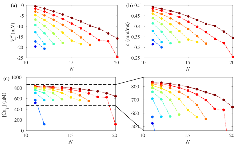
Figure 9: Selected biomarkers of myocyte action potentials propagating down myocyte straits (2.3c) as functions of the strait width $\Delta y$ and the number of fibroblasts $N$ coupled to each myocyte in the flanking regions. Dotted lines connect points with identical values of $\Delta y$ increasing from 0.1 mm to 0.9 mm in increments of 0.1mm from bottom (blue color) to top (dark red color). (a) Peak myocyte potential, (b) wave speed and (c) peak calcium concentration in the middle of the straits at $y=L/2$.

4 Asymptotic theory for the case of uniform fibroblast distribution

In this section we extend the asymptotic theory of (Simitev & Biktashev,, 2006; Biktashev et al.,, 2008; Simitev & Biktashev,, 2011) to the case C1 of uniform fibroblast distribution. The theory captures qualitatively the behaviour of action potential biomarkers reported above and explains the occurrence of propagation block with increasing fibroblast count $N$.

4.1 Formulation of a periodic boundary value problem

In the uniform case the fibroblast distribution takes the simple form $n(x,y)=N$ and, by symmetry, we can neglect the dependence on the $y$-coordinate and reduce problem (2.1) to one spatial dimension. Further, to investigate action potentials excited by a periodic stimulus (2.2) and propagating with a fixed shape and a constant speed $c$, we introduce a travelling wave ansatz $z=\tilde{x}+ct$, where $\tilde{x}=x\sqrt{C_{\text{m}}\chi/\sigma_{11}}$ is a rescaled $x$ coordinate, and arrive at the periodic boundary value problem

$$c\frac{d}{dz}V_{\text{m}} =-\frac{1}{C_{\text{m}}}\Big{(}I_{\text{m}}(V_{\text{m}},\mathbf{u})+N\,G_{\text{gap}}(V_{\text{m}}-V_{\text{f}})\Big{)}+\frac{d^{2}}{dz^{2}}V_{\text{m}},$$ (4.1a)

$$c\frac{d}{dz}V_{\text{f}} =-\frac{1}{C_{\text{f}}}\Big{(}I_{\text{f}}(V_{\text{f}},\mathbf{u})+G_{\text{gap}}(V_{\text{f}}-V_{\text{m}})\Big{)},$$ (4.1b)

$$c\frac{d}{dz}\mathbf{u} =\mathbf{F}(\mathbf{u},V_{\text{m}},V_{\text{f}}),$$ (4.1c)

$$V_{\text{m}}(0) =V_{\text{m}}(cB),\;\frac{d}{dz}V_{\text{m}}(0)=\frac{d}{dz}V_{\text{m}}(cB),\;V_{\text{m}}(z_{0})=V_{\text{m}}^{b},\;V_{\text{f}}(0)=V_{\text{f}}(cB),\;\mathbf{u}(0)=\mathbf{u}(cB),$$ (4.1d)

where $\mathbf{u}$ is a vector of all gating variables controlling the permittivity of myocyte and fibroblast ionic channels and of all intra- and extra-cellular concentrations of ions and $\mathbf{F}$ are the functions controlling their dynamics as defined in (Courtemanche et al.,, 1998) and (Morgan et al.,, 2016) and also specified in further detail below. The condition $V_{\text{m}}(z_{0})=V_{\text{m}}^{b}$ is a “phase/pinning” condition required to eliminate the translational invariance of the system and arises as a replacement of the initial value condition present in problem (2.1); here $z_{0}\in[0,cB]$ and $V_{\text{m}}^{b}$ is an arbitrary constant within range of $V_{\text{m}}$, e.g. $V_{\text{m}}^{b}=0$ mV.

4.2 Asymptotic embedding

For the analysis of the eigen-boundary value problem formulated above, we follow an asymptotic embedding procedure described in (Biktashev et al.,, 2008) and introduce in equations (4.1) a parameter $\epsilon>0$ such that for $\epsilon=1$ the embedding is identical to (4.1) while in the limit $\epsilon\to 0^{+}$ useful asymptotic simplifications are obtained. There are infinitely many ways to embed a small parameter $\epsilon$ and their merits are assessed (a) on the basis of the usefulness of the asymptotic simplifications and (b) on the quality of approximation to the solutions of the original problem. The asymptotic embedding of equations (4.1) used below is based on our earlier study (Simitev & Biktashev,, 2006) of the relative speed of the dynamical variables in the atrial model of Courtemanche et al., (1998). For a system of $M$ differential equations $\mathrm{d}{{w}_{l}}/\mathrm{d}{{t}}={F}_{l}({w}_{1},\dots w_{M})$, ${l}=1,\dots M$ the relative speeds of dynamical variables ${w}_{l}$ can be formally measured by their time-scaling functions defined as ${\tau_{{l}}}({w}_{1},\ldots)\equiv\left|\mathrm{d}{{F}_{{l}}}/\mathrm{d}{{w}_{{l}}}\right|^{-1}$, ${l}=1\ldots M$. Comparing relevant time-scaling functions, our earlier work established that the myocyte potential $V_{\text{m}}$ and the gating variables $m$ and $h$ are “fast variables”, i.e. they change significantly during the upstroke of a typical action potential, while all other variables are “slow” as they change only weakly during that period. However, an unusual non-Tikhonov, (1952) feature of the system is that $V_{\text{m}}$ is both fast and slow. The potential $V_{\text{m}}$ is only fast because of the presence of a large sodium current $g_{\text{Na}}(V_{\text{Na}}-V_{\text{m}})jhm^{3}$. In turn, the sodium current is large only during the upstroke of the action potential but not large otherwise. This is due to the near perfect switch behaviour of gates ${m}$ and ${h}$ which are almost fully closed outside the upstroke. These observations lead us to adopt the following asymptotic embedding of equations (4.1)

$$c\frac{d}{dz}V_{\text{m}} =-\frac{1}{C_{\text{m}}}\Big{(}\frac{1}{\epsilon}g_{\text{Na}}(V_{\text{Na}}-V_{\text{m}})jhm^{3}+I_{\Sigma}(V_{\text{m}},j,\mathbf{u}_{\text{m}})+N\,G_{\text{gap}}(V_{\text{m}}-V_{\text{f}})\Big{)}+\epsilon\frac{d^{2}}{dz^{2}}V_{\text{m}},$$ (4.2a)

$$c\frac{d}{dz}V_{\text{f}} =-\frac{1}{C_{\text{f}}}\Big{(}I_{\text{f}}(V_{\text{f}},\mathbf{u}_{\text{f}})+G_{\text{gap}}(V_{\text{f}}-V_{\text{m}})\Big{)},$$ (4.2b)

$$c\frac{d}{dz}m =\frac{\bar{m}(V_{\text{m}},\epsilon)-m}{\epsilon\tau_{m}(V_{\text{m}})},\quad\bar{m}(V_{\text{m}},0)=H(V_{\text{m}}-E_{m}),$$ (4.2c)

$$c\frac{d}{dz}h =\frac{\bar{h}(V_{\text{m}},\epsilon)-h}{\epsilon\tau_{h}(V_{\text{m}})},\quad\bar{h}(V_{\text{m}},0)=H(E_{h}-V_{\text{m}}),$$ (4.2d)

$$c\frac{d}{dz}j =\frac{\bar{j}(V_{\text{m}})-j}{\tau_{j}(V_{\text{m}})},$$ (4.2e)

$$c\frac{d}{dz}\begin{bmatrix}\mathbf{u}_{\text{m}}\\ \mathbf{u}_{\text{f}}\end{bmatrix} =\begin{bmatrix}\mathbf{T}_{\text{m}}(V_{\text{m}})&0\\ 0&\mathbf{T}_{\text{f}}(V_{\text{f}})\end{bmatrix}\left(\begin{bmatrix}\overline{\mathbf{u}_{\text{m}}}(V_{\text{m}})\\ \overline{\mathbf{u}_{\text{f}}}(V_{\text{f}})\end{bmatrix}-\begin{bmatrix}\mathbf{u}_{\text{m}}\\ \mathbf{u}_{\text{f}}\end{bmatrix}\right).$$ (4.2f)

The current $I_{\Sigma}$ is the sum of all slow currents and $\mathbf{u}_{\text{m}}$ and $\mathbf{u}_{\text{f}}$ are vectors composed of the remaining slow gating variables (in addition to $j$ which is also slow) with myocyte and fibroblast kinetics, respectively. The functions $\tau_{w}$ and $\bar{w}$ are time-scaling functions and quasi-stationary values of gating variables $w=j,m,h$, respectively. For the remaining slow gates these time scaling functions are arranged in diagonal matrices $\mathbf{T}_{\text{m}}$ and $\mathbf{T}_{\text{f}}$ with indices denoting myocyte and fibroblast function and $\overline{\mathbf{u}_{\text{m}}}$ and $\overline{\mathbf{u}_{\text{f}}}$ are quasi-stationary values. The explicit forms of these expressions are specified in (Courtemanche et al.,, 1998; Morgan et al.,, 2016). To account for the perfect switch behaviour of $m$ and $h$, the functions $\bar{m}(V_{\text{m}},\epsilon)$ and $\bar{h}(V_{\text{m}},\epsilon)$ are “embedded”, i.e. they are ${\epsilon}$-dependent versions of $\bar{m}(V_{\text{m}})$ and $\bar{h}(V_{\text{m}})$ such that $\bar{m}(V_{\text{m}};1)=\bar{m}(V_{\text{m}})$ and $\bar{h}(V_{\text{m}};1)=\bar{h}(V_{\text{m}})$ on one hand and $\bar{m}(V_{\text{m}},0)=H(V_{\text{m}}-E_{m})$ and $\bar{h}(V_{\text{m}},0)=H(E_{h}-V_{\text{m}})$ on the other hand, with ${{E}_{m}}=-32.7\,\mathrm{mV}$ and ${{E}_{h}}=-66.66\,\mathrm{mV}$ so that $\bar{m}({{E}_{m}})=1/2$ and $\bar{h}({{E}_{h}})=1/2$.

4.3 Asymptotic reduction

We are now ready to exploit the asymptotic embedding (4.2). Rescaling $Z=z/\epsilon$, taking the limit $\epsilon\to 0^{+}$ and neglecting decoupled equations, we obtain the fast-time subsystem

$$c\frac{d}{dZ}V_{\text{m}} =-\frac{g_{\text{Na}}j^{\alpha}}{C_{\text{m}}}(V_{\text{Na}}-V_{\text{m}})hm^{3}+\frac{d^{2}}{dZ^{2}}V_{\text{m}},$$ (4.3a)

$$c\frac{d}{dZ}m =\frac{H(V_{\text{m}}-E_{m})-m}{\tau_{m}(V_{\text{m}})},$$ (4.3b)

$$c\frac{d}{dZ}h =\frac{H(E_{h}-V_{\text{m}})-h}{\tau_{h}(V_{\text{m}})},$$ (4.3c)

$$V_{\text{m}}(-\infty) =V_{\text{m}}^{\alpha},\;\frac{d}{dZ}V_{\text{m}}(\infty)=0,\;V_{\text{m}}(\infty)=V_{\text{m}}^{\omega},\;V_{\text{m}}(0)={{E}_{h}},\;m(-\infty)=0,\;h(-\infty)=1.$$ (4.3d)

To avoid ambiguity we have specified in (4.3d) the pinning condition explicitly at $Z=0$ and have taken $Z$ in the range $Z\in(-\infty,\infty)$. We have also introduced the post-front potential, $V_{\text{m}}^{\omega}$ as a new parameter and introduced a condition to constrain it. We note that fibroblast kinetics does not explicitly affect this fast-time subsystem making this very similar to the problem considered in (Simitev & Biktashev,, 2006). Taking the limit $\epsilon\to 0^{+}$ directly in equations (4.2) and noting that at time scales much longer than $\epsilon$, the third and fourth equations imply that the sodium current in equation (4.2a) is proportional to $H(V_{\text{m}}-E_{m})H(E_{h}-V_{\text{m}})=0$ which vanishes in the limit $\epsilon\to 0^{+}$ despite the large factor $\epsilon^{-1}$ in front of it, we obtain the slow-time subsystem

$$c\frac{d}{dz}V_{\text{m}} =-\frac{1}{C_{\text{m}}}\Big{(}I_{\Sigma}(V_{\text{m}},j,\mathbf{u}_{\text{m}})+N\,G_{\text{gap}}(V_{\text{m}}-V_{\text{f}})\Big{)},$$ (4.4a)

$$c\frac{d}{dz}V_{\text{f}} =-\frac{1}{C_{\text{f}}}\Big{(}I_{\text{f}}(V_{\text{f}},\mathbf{u}_{\text{f}})+G_{\text{gap}}(V_{\text{f}}-V_{\text{m}})\Big{)},$$ (4.4b)

$$c\frac{d}{dz}j =\frac{\bar{j}(V_{\text{m}})-j}{\tau_{j}(V_{\text{m}})},$$ (4.4c)

$$c\frac{d}{dz}\begin{bmatrix}\mathbf{u}_{\text{m}}\\ \mathbf{u}_{\text{f}}\end{bmatrix} =\begin{bmatrix}\mathbf{T}_{\text{m}}(V_{\text{m}})&0\\ 0&\mathbf{T}_{\text{f}}(V_{\text{f}})\end{bmatrix}\left(\begin{bmatrix}\overline{\mathbf{u}_{\text{m}}}(V_{\text{m}})\\ \overline{\mathbf{u}_{\text{f}}}(V_{\text{f}})\end{bmatrix}-\begin{bmatrix}\mathbf{u}_{\text{m}}\\ \mathbf{u}_{\text{f}}\end{bmatrix}\right),$$ (4.4d)

$$V_{\text{m}}(0) =V_{\text{m}}^{\omega},\;V_{\text{m}}(cB)=V_{\text{m}}^{\alpha},\;V_{\text{f}}(0)=V_{\text{f}}(cB),\;j(0)=j^{\alpha},\;j(cB)=j^{\alpha},$$

$$\mathbf{u}_{\text{m}}(0) =\mathbf{u}_{\text{m}}(cB),\;\mathbf{u}_{\text{f}}(0)=\mathbf{u}_{\text{f}}(cB).$$ (4.4e)

For a specified period of stimulation $B$, fibroblast count $N$ and other myocyte and fibroblast parameter values, e.g. $C_{\text{m}}$, $C_{\text{f}}$, $G_{\text{gap}}$, $g_{\text{Na}}$ etc., that are all fixed as in (Courtemanche et al.,, 1998; Morgan et al.,, 2016), the coupled fast-time and slow-time systems (4.3) and (4.4) have differential equations of cumulative order $7+\dim(\mathbf{u}_{\text{m}})+\dim(\mathbf{u}_{\text{f}})$ and contain 4 free parameters ($c$, $V_{\text{m}}^{\alpha}$, $V_{\text{m}}^{\omega}$, $j^{\alpha}$), on one hand, and on the other hand, feature $10+\dim(\mathbf{u}_{\text{m}})+\dim(\mathbf{u}_{\text{f}})$ boundary conditions and 1 pinning condition. Therefore, the solution of (4.3) and (4.4), or equivalently of (4.1), is fully determined and can be found using numerical methods for solution of boundary value problems, see (Simitev & Biktashev,, 2011). In particular, components such as $c(N)$ and $V_{\text{m}}^{\omega}(N)$can be computed to compare with biomarkers from direct numerical simulations shown in Fig. 4. However, in order to understand the solutions more explicitly we next consider the fast-time and the slow-time problems separately from each other.

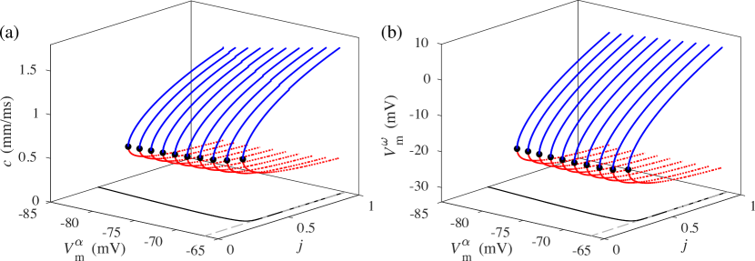
Figure 10: Selected components of the solution to the fast-time system (4.3) computed using the numerical method of Simitev & Biktashev, (2006). (a) Wave speed $c$ and (b) peak myocyte potential $V_{\text{m}}^{\omega}$ both as two-valued functions of the pre-front values of the myocyte potential $V_{\text{m}}^{\alpha}$ and of the slow inactivation gating variable of the myocyte sodium current $j^{\alpha}$. The critical curve $j^{\alpha}_{\text{crit}}(V_{\text{m}}^{\alpha})$ below which the fast-time problem has no solutions is shown as a black curve in the $(V_{\text{m}}^{\alpha}-j^{\alpha})$-plane in both panels.

4.4 Solution to the fast-time system

For fixed myocyte and fibroblast parameter values, the fast-time system (4.3) has differential equations of cumulative order four and contains four free parameters ($c$, $V_{\text{m}}^{\alpha}$, $V_{\text{m}}^{\omega}$, $j^{\alpha}$), while being constraint by five boundary conditions and one pinning condition. Therefore, the fast-time system is expected to have a two-parameter family of solutions, meaning that two of the free parameters can be chosen arbitrarily and all components of the solution will be functions of these two. For comparison with the direct numerical simulations shown in Fig. 4, we choose the prefront values of the myocyte potential $V_{\text{m}}^{\alpha}$ and of the slow inactivation gating variable of the myocyte sodium current $j^{\alpha}$ as independent parameters. Fig. 10 shows the wave speed and the post-front myocyte potential as functions of the latter two,

$$c=c(V_{\text{m}}^{\alpha},j^{\alpha}),\quad V_{\text{m}}^{\omega}=V_{\text{m}}^{\omega}(V_{\text{m}}^{\alpha},j^{\alpha}),$$ (4.5)

respectively. The solutions are computed using the numerical method of Simitev & Biktashev, (2006) where a problem identical to (4.3) save a curvature effect term was considered. The numerics take into account that the fast-time problem is posed on an infinite interval and that its right-hand sides are piece-wise differentiable. Fig. 10 shows that solutions of the fast-time problem exist only within a certain region of the $(V_{\text{m}}^{\alpha}-j^{\alpha})$-plane above a critical curve $j^{\alpha}_{\text{crit}}(V_{\text{m}}^{\alpha})$. In particular, at every point within this region two distinct solutions can be found – one solution sitting in a stable branch corresponding to a faster speed $c_{1}$ and an one solution sitting in an unstable branch corresponding to a slower speed $c_{2}$. Other solution components are similarly two-valued functions of $V_{\text{m}}$ and $j^{\alpha}$. A more rigorous demonstration of these assertions can be found in (Simitev & Biktashev,, 2011) where closed-form analytical solutions are presented for a conceptual model with a similar asymptotic structure. For the particular atrial kinetics of Courtemanche et al., (1998) considered here, a regular perturbation approximation of the critical curve $j^{\alpha}_{\text{crit}}(V_{\text{m}}^{\alpha})$ and of the wave speed $c$ has been reported in (Simitev & Biktashev,, 2006) and a solution in terms of iterated integral expressions has been presented in (Simitev & Biktashev,, 2008).

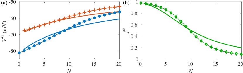
Figure 11: Selected components of the equilibrium solution to the slow-time system (4.7). (a) The resting (pre-front) myocyte potential $V_{\text{m}}^{\alpha}$ (solid blue curve) and fibroblast potential $V_{\text{f}}^{\alpha}$ (solid red curve) as functions of the fibroblast count $N$ evaluated from (4.10). Dotted curves with blue circle markers and with red plus-sign markers show values of $V_{\text{m}}^{\alpha}$ and $V_{\text{f}}^{\alpha}$, respectively, measured from direct numerical simulations of (2.1) as discussed in Section 3.1. (b) The resting (pre-front) value $j^{\alpha}$ of the $j$-gate as a function of the fibroblast count $N$ evaluated analytically (solid green curve) and from direct numerical simulations (dotted curve with diamond markers). Parameter values are specified in Table 1 with $B\to\infty$, and $G_{\text{f}}=0.23$ nS and $G_{\text{m}}=2.2$ nS.

4.5 Equilibrium solution of the slow-time system

For fixed myocyte and fibroblast parameter values, the slow-time system (4.4) has differential equations of cumulative order $3+\dim(\mathbf{u}_{\text{m}})+\dim(\mathbf{u}_{\text{f}})$ and contains four free parameters ($c$, $V_{\text{m}}^{\alpha}$, $V_{\text{m}}^{\omega}$, $j^{\alpha}$), while being constraint by $5+\dim(\mathbf{u}_{\text{m}})+\dim(\mathbf{u}_{\text{f}})$ boundary conditions. However, wave speed $c$ is not an essential unknown as it can be eliminated by rescaling the independent variable and, therefore the slow-time system is expected to have a one-parameter family of solutions. A natural choice for the independent free parameter is the initial value of the myocyte potential $V_{\text{m}}^{\omega}$, which would then, in principle, allow to determine all slow-time solution components, for instance,

$$V_{\text{m}}^{\alpha}=V_{\text{m}}^{\alpha}(V_{\text{m}}^{\omega}),\quad j^{\alpha}=j^{\alpha}(V_{\text{m}}^{\omega}).$$ (4.6)

We note that the fibroblast kinetics is now an essential part of the slow-time problem and the solutions also depend on other model parameters in particular the fibroblast count $N$. The slow myocyte and fibroblast kinetics of (Courtemanche et al.,, 1998; Morgan et al.,, 2016) are given by multi-component nonlinear expressions and analytical solutions to problem (4.4) are not known. To make further progress, we will restrict the attention to finding the equilibrium state of the slow-time system. This is sufficient to estimate wave speed and peak myocyte potential needed for comparison to the direct numerical experiments reported in Section 3.1, as well as to understand the failure of propagation in the case of a single action potential excited by a stimulus of infinite period $B\to\infty$, and propagating into a fully rested tissue.

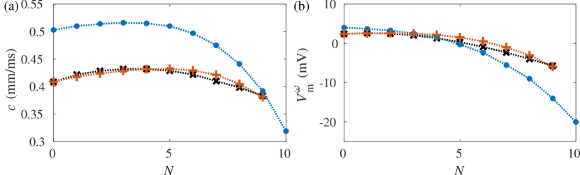
Figure 12: Selected components of the solution to the coupled fast- and slow-time problems. (a) Wave speed $c$ and (b) peak myocyte potential $V_{\text{m}}^{\omega}$ as functions of fibroblast count $N$ for parameter values specified in Table 1, $B\to\infty$ and $G_{\text{f}}=0.23$ nS and $G_{\text{m}}=2.24$ nS. Results from solution of (4.3) by the numerical method of (Simitev & Biktashev,, 2006) coupled to expressions (4.10) and (4.8) are denoted by black cross-sign markers. Results from direct numerical simulations of (2.1) are denoted with blue circle markers. Results from solution of (4.3) by the numerical method of (Simitev & Biktashev,, 2006) coupled to $V_{\text{m}}^{\alpha}$ and $j^{\alpha}$ measured from direct numerical simulations are denoted by red plus-sign markers.

The equilibrium state of the slow-time problem (4.4) is determined by

$$0 =I_{\Sigma}(V_{\text{m}},j,\mathbf{u}_{\text{m}})+N\,G_{\text{gap}}(V_{\text{m}}-V_{\text{f}}),$$ (4.7a)

$$0 =I_{\text{f}}(V_{\text{f}},\mathbf{u}_{\text{f}})+G_{\text{gap}}(V_{\text{f}}-V_{\text{m}}),$$ (4.7b)

$$0 =\bar{j}(V_{\text{m}})-j,$$ (4.7c)

$$0 =\overline{\mathbf{u}_{\text{m}}}(V_{\text{m}})-\mathbf{u}_{\text{m}},$$ (4.7d)

$$0 =\overline{\mathbf{u}_{\text{f}}}(V_{\text{f}})-\mathbf{u}_{\text{f}}.$$ (4.7e)

Equations (4.7c), (4.7d) and (4.7e) can be solved immediately,

$$j^{\alpha}=\bar{j}(V_{\text{m}}),\quad\mathbf{u}_{\text{m}}^{\alpha}=\overline{\mathbf{u}_{\text{m}}}(V_{\text{m}}),\quad\mathbf{u}_{\text{f}}^{\alpha}=\overline{\mathbf{u}_{\text{f}}}(V_{\text{f}}),$$ (4.8)

and gating variables can be then eliminated from the potential equations (4.7a) and (4.7b). The latter are now involved non-linear functions of $V_{\text{m}}$ and $V_{\text{f}}$ alone and linearisation near the resting potentials $V_{\text{m}}^{0}=-81$ mV and $V_{\text{f}}^{0}=-46$ mV of the decoupled myocyte and fibroblast models yields

$$0 =I_{\Sigma}(V_{\text{m}})+N\,G_{\text{gap}}(V_{\text{m}}-V_{\text{f}})\approx G_{\text{m}}(V_{\text{m}}-V_{\text{m}}^{0})+NG_{\text{gap}}(V_{\text{m}}-V_{\text{f}}),$$ (4.9a)

$$0 =I_{\text{f}}(V_{\text{f}})+G_{\text{gap}}(V_{\text{f}}-V_{\text{m}})\approx G_{\text{f}}(V_{\text{f}}-V_{\text{f}}^{0})+G_{\text{gap}}(V_{\text{f}}-V_{\text{m}}),$$ (4.9b)

where $G_{\text{m}}=[dI_{\Sigma}/dV_{\text{m}}]_{V_{\text{m}}^{0}}\approx 2.2$ nS, $G_{\text{f}}=[dI_{\text{f}}/dV_{\text{f}}]_{V_{\text{f}}^{0}}\approx 0.23$ nS, and where we have taken into account that the currents $I_{\Sigma}(V_{\text{m}}^{0})$ and $I_{\text{f}}(V_{\text{f}}^{0})$ vanish by the definition of $V_{\text{m}}^{0}$ and $V_{\text{f}}^{0}$. Solutions to the linear set (4.9) are then easily obtained

$$V_{\text{m}}^{\alpha}(N) =V_{\text{m}}^{0}+N(V_{\text{f}}^{0}-V_{\text{m}}^{0})/\big{(}G_{\text{m}}(G_{\text{gap}}^{-1}+G_{\text{f}}^{-1}+NG_{\text{m}}^{-1})\big{)},$$ (4.10a)

$$V_{\text{f}}^{\alpha}(N) =V_{\text{f}}^{0}-(V_{\text{f}}^{0}-V_{\text{m}}^{0})/\big{(}G_{\text{f}}(G_{\text{gap}}^{-1}+G_{\text{f}}^{-1}+NG_{\text{m}}^{-1})\big{)},$$ (4.10b)

and equilibrium values of $j$ and other gating variables are subsequently found from equations (4.8). Expressions (4.10) and (4.8) are plotted in Fig. 11. The analytical results are compared in the figure with values of $V_{\text{m}}^{\alpha}$, $V_{\text{f}}^{\alpha}$, and $j^{\alpha}$ measured from direct numerical simulations of (2.1) as discussed in Section 3.1 and demonstrate accuracy adequate for the goals of this analysis.

Figure 13: Critical fibroblast count $N_{\text{crit}}$ beyond which propagation failure occurs. The thick solid black curve is the critical refractoriness boundary curve $j^{\alpha}_{\text{crit}}(V_{\text{m}}^{\alpha})$ for the existence of solutions to the fast-time system as also shown in Fig. 10. The blue curve is the locus of pairs of equilibrium values of the $j$-gate and the myocyte potential $\big{(}V_{\text{m}}^{\alpha}(N),j^{\alpha}(N)\big{)}$ for fibroblast counts $N$ as denoted by circle markers along the curve. The value of $N$ at the intersection point marked with an asterisk is the critical fibroblast count $N_{\text{crit}}\approx=9.8$. Parameter values are specified in Table 1 with $B\to\infty$, and $G_{\text{f}}=0.23$ nS and $G_{\text{m}}=2.2$ nS.

4.6 Coupling and conditions for propagation

The equilibrium solution of the slow-time system can now be coupled to the solution of the fast-time system. The resting myocyte potential $V_{\text{m}}^{\alpha}$ and the resting value of the slow inactivation gating variable of the myocyte sodium current $j^{\alpha}$ in the tissue serve as pre-front values for the propagating wave front. Hence, substituting expressions (4.10) and (4.8) into equations (4.5) we find the wave speed and the peak myocyte potential as functions of the fibroblast count $N$ (and other model parameters),

$$c=c\big{(}V_{\text{m}}^{\alpha}(N),j^{\alpha}(N)\big{)},\qquad V_{\text{m}}^{\omega}=V_{\text{m}}^{\omega}\big{(}V_{\text{m}}^{\alpha}(N),j^{\alpha}(N)\big{)}.$$ (4.11)

In practice, expressions (4.10) and (4.8) are first used to approximate $V_{\text{m}}^{\alpha}(N)$ and $j^{\alpha}(N)$ and these are then used as inputs to the fast-time boundary value problem (4.3) which is solved by the numerical method of (Simitev & Biktashev,, 2006). These asymptotic results are plotted in Fig. 12 and compared with the wave speed and the peak myocyte potential measured from direct numerical simulations of the monodomain tissue equations (2.1) performed as described in section as discussed in Section 3.1. The relative error between the asymptotic approximation to the wave speed and the values from the direct numerical simulations is approximately 19% at $N=0$ and decreases with increasing $N$. To split the error contributions due to the asymptotic reduction from those due to the linearisation of currents near the resting state, we have also plotted in Fig. 12 curves computed using pre-front values $V_{\text{m}}^{\alpha}$ and $j^{\alpha}$ obtained from direct numerical simulations rather than from expressions (4.10) and (4.8) but still solving the fast-time boundary value problem. Errors due to the asymptotic reduction dominate.

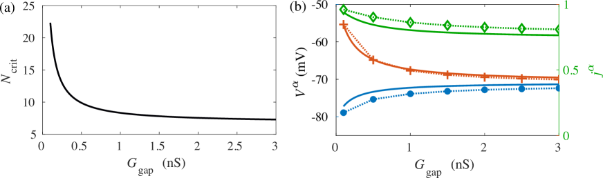
Figure 14: Dependence on myocyte-fibroblast coupling conductance $G_{\text{gap}}$. (a) Minimal number of coupled fibroblasts necessary for propagation $N_{\text{crit}}$ computed from equation (4.12). (b) Resting (pre-front) potentials and $j$ gate values computed from (4.10) and (4.8) as well as from direct numerical simulations. Same formatting conventions as in Fig. 11 are used with $V_{\text{m}}^{\alpha}$ and $V_{\text{f}}^{\alpha}$ on the left $y$-axis and $j^{\alpha}$ on the right $y$-axis. Fibroblast count is fixed to ${N}=4$ in (b). In (a) and (b), other parameter values are as specified in Table 1 with $B\to\infty$ and $G_{\text{f}}=0.23$ nS and $G_{\text{m}}=2.2$ nS.

With the insight from the asymptotic reduction and consequent coupling, the occurrence of propagation failure with increasing fibroblast count can now be easily understood. Propagating front solutions to the fast-time system (4.3) exist if and only if a point $(V_{\text{m}}^{\alpha},j^{\alpha})$, with abscissa given by the value of the pre-front myocyte potential and ordinate given the pre-front value of the slow inactivation gating variable of the myocyte sodium current $j$, belongs to the region in the $(V_{\text{m}},j)$-plane located above the critical bifurcation curve $j^{\alpha}_{\text{crit}}(V_{\text{m}}^{\alpha})$ as plotted in Fig. 10 while propagating front solutions do not exist in the region under the curve. The $j^{\alpha}_{\text{crit}}(V_{\text{m}}^{\alpha})$ curve, therefore serves as the boundary between absolute and relative refractoriness, i.e. the boundary between the ability and the inability of the medium to conduct excitation waves. Refractoriness is a fundamental characteristic of biological excitable media, including cardiac tissues. On the other hand, for a given fibroblast count $N$, the values of $V_{\text{m}}^{\alpha}$ and $j^{\alpha}$ are determined from the solution of the slow-time system (4.4). In the special case of propagation of a single action potential through a rested tissue, these are given by equations (4.10) and (4.8) for the equilibrium values of myocyte potential and the slow inactivation gating variable of the myocyte sodium current. Therefore, propagation is possible if these values fall within the region of relative refractoriness above the critical curve $j^{\alpha}_{\text{crit}}(V_{\text{m}}^{\alpha})$ and failure occurs if these values fall within the region of absolute refractoriness below $j^{\alpha}_{\text{crit}}(V_{\text{m}}^{\alpha})$. In Fig. 13 the $j^{\alpha}_{\text{crit}}(V_{\text{m}}^{\alpha})$ as well as the curve $\big{(}V_{\text{m}}^{\alpha}(N),j^{\alpha}(N)\big{)}$ parametrised by the fibroblast count $N$ are plotted together in the $(V_{\text{m}},j)$ plane for the standard set of parameter values given in Table 1. The intersection of these two curves determines the critical fibroblast count $N_{\text{crit}}$ beyond which propagation failure occurs. The $N_{\text{crit}}$ is denoted in Fig. 13 and is bracketed between $N=9$ and $N=10$ in full agreement with the results from direct numerical simulations, see Fig. 4 and discussion in Section 3.1. Fig. 13 also indicates that the intersection between the two curves occurs at a point far along the vertical asymptote $V_{\text{m}}^{\alpha}={{E}_{h}}$ of the fast-time system critical curve $j^{\alpha}_{\text{crit}}(V_{\text{m}}^{\alpha})$. This observation allows us to derive an explicit expression for the critical fibroblast count as a function of the parameters of the problem. Indeed, the algebraic equation $V_{\text{m}}^{\alpha}={{E}_{h}}$, where $V_{\text{m}}^{\alpha}$ is given by (4.10) and ${{E}_{h}}=-66.6$ mV, is linear in $N$ and solving his equation we find the approximation

$$N_{\text{crit}}=\frac{G_{\text{m}}\,(G_{\text{f}}+G_{\text{gap}})\,{{({{E}_{h}}-V_{\text{m}}^{0})}}}{G_{\text{f}}G_{\text{gap}}\,{{(V_{\text{f}}^{0}-{{E}_{h}})}}}.$$ (4.12)

It follows directly from equation (4.12) that propagation is always possible for values of the uncoupled fibroblast resting potential smaller than ${{E}_{h}}$, i.e. when $V_{\text{f}}^{0}<{{E}_{h}}$. This is significant since a range of experimental values have been reported for this parameter, e.g. (Chilton et al.,, 2005). Specific biomarker values reported from the direct numerical simulations in Section 3 also depend on the rest of the model parameters. Another model parameter with value poorly constrained from experiments is the myocyte-fibroblast coupling conductance $G_{\text{gap}}$. In the above, the value of $G_{\text{gap}}$ was chosen largely for numerical convenience. Now, with the help of the asymptotic theory developed here the dependence on myocyte-fibroblast coupling conductance $G_{\text{gap}}$ can be constructed easily. Fig. 14(a) shows the critical number of coupled fibroblasts $N_{\text{crit}}$ as a function of the value of myocyte-fibroblast coupling conductance $G_{\text{gap}}$ plotted from expression (4.12). Fig. 14(b) shows the variation of the resting coupled myocyte and fibroblast potentials and the resting value of the slow inactivation gating variable of the myocyte sodium current $j$ with variation of $G_{\text{gap}}$ computed from equations (4.10) and (4.8). Results from direct numerical simulations of the uniformly distributed fibroblast case at fixed $N=4$ are also plotted there and show excellent agreement. This serves to demonstrate that the asymptotic theory remains qualitatively valid. It has been too expensive to compute the entire critical curve as a function of $G_{\text{gap}}$ by direct simulations. We believe that the conceptual interpretation and the qualitative conclusions of the asymptotic theory remain true for a wide range of parameters, in the same way as for the variation with $G_{\text{gap}}$.

5 Summary and conclusions

Cardiac fibroblasts are the most abundant type of non-myocyte cells in the myocardium. They perform various functions, differ widely in phenotype and are known to be electrically active. Fibroblasts connect to myocytes via gap junctional channels and evidence exists that direct electrical interaction between the two types of cells can have arrhythmogenic effects. In this article we perform (a) direct numerical simulations, as well as (b) an asymptotic analysis of action potential propagation and block, in a model of atrial tissue with myocyte-fibroblast coupling. This is done with the aim to understand conduction disturbances, spatially non-uniform conduction and conduction block all of which are thought to be key elements in the initiation and sustenance of arrhythmias.

We consider a mathematical model of fibrous atrial tissue formulated in terms of a set of cardiac monodomain equations including a myocyte-fibroblast coupling current. Following the work of Xie et al., 2009b , we adopt an “attachment” approach to couple the human atrial myocyte model of Courtemanche et al., (1998) to the mammalian fibroblast model of Morgan et al., (2016). A key advantage of the “attachment” approach is that it can be easily employed within a homogenised continuum model such as the monodomain equations and a variety of fibroblast distributions can be prescribed simply and acutely. The alternative “insertion” approach requires that the model is defined on a discrete grid and does not lend itself easily to asymptotic analysis of the type report here. The atrial model of Courtemanche et al., (1998) is chosen as partial asymptotic results were readily available in our earlier work (Simitev & Biktashev,, 2006) for its specific kinetics and because our numerical code was already validated in this case against the benchmark of Niederer et al., (2011). For direct numerical simulations of the monodomain equations we use the Strang operator splitting method.

Using this setup we investigate three idealised fibroblast distributions: uniform distribution, fibroblast barrier distribution and myocyte strait distribution, that we hypothesize are constituent blocks of realistic fibroblast distributions. Essential action potential biomarkers that are typically measured in electrophysiological myocardial tissue experiments including conduction velocity, peak potential, action potential duration, and triangulation index are estimated from direct numerical simulations for all idealised distributions. Failure of action potential propagation is found to occur at certain critical values of the parameters that define each of the idealised fibroblast distributions and these critical values are accurately determined. In the case of uniform fibroblast distribution we find that electrical excitation fails to propagate when 10 or more fibroblasts are coupled to each myocyte at the standard parameter values of our simulations. As fibroblast count increases from zero, peak potential decreases while conduction velocity slightly increases for moderate fibroblast count $N$ and then as $N$ increases further a block occurs. The values of APD₉₀ increase as the fibroblast count increases until close to the propagation threshold when APD₉₀ decreases rapidly. Similarly, the calcium concentration stays relatively constant as $N$ increases from 0, until $N=8$, after which it also falls off rapidly. In the case of fibroblast barrier where “healthy” tissue is separated by a region of increased fibroblast count our direct numerical simulations show that propagation block is determined by both the width of the fibroblast barrier and the count of fibroblasts coupled to each myocyte within it. For examples, the larger the count of coupled fibroblasts within the region the thinner it must be to allow successful AP propagation. We proceed to determine a threshold curve of fibroblast count versus width that splits propagation from failure. This curve is akin to strength-duration curves that are used elsewhere to determine the amplitude and the duration of a stimulus current that is needed to trigger excitation. Unlike in the first and third fibroblast distribution cases, in this second case, it is not appropriate to measure biomarkers as the barrier region is not big enough. In the case of myocyte strait where channel of “healthy” tissue between two regions of increased fibroblast count we demonstrate that successful AP depends on both the width of the strait and the fibroblast count in the adjacent regions. For instance, the larger the count of coupled fibroblasts in the surrounding regions is, the wider the strand must be to admit the pulse across. Similarly, to the second case we construct a threshold curve of fibroblast count versus strait width that splits propagation from failure. When the strait width is held constant, as the fibroblast density in the adjacent regions increases the wave speed, peak potential and the peak calcium concentration all decrease.

To explain these direct numerical simulation results we extend and apply an asymptotic theory in our earlier works (Simitev & Biktashev,, 2011) to the case of uniform fibroblast distribution. Action potential biomarkers values are obtained as hybrid analytical-numerical solutions of coupled fast-time and slow-time periodic boundary value problems and compare well to direct numerical simulations. The boundary of absolute refractoriness is determined solely by the fast-time problem and is found to depend on the values of the myocyte potential and the slow inactivation variable of the sodium current ahead of the propagating front of the action potential. These quantities are in turn estimated from the slow-time problem using a regular perturbation expansion to find the steady state of the coupled myocyte-fibroblast kinetics. The asymptotic theory captures with remarkable accuracy the block of propagation in the presence of fibroblasts.

Our work does not consider the effect of collagen formed in the fibrotic scar. This has been excluded here as collagen is not electrically active and thus its main contribution is to alter the value of the effective diffusivity and this can be accounted for by simply rescaling the spatial variables in the governing equations. While this is straightforward in theory, it is difficult in practise to distinguish the effects of myocyte-fibroblast coupling we report here from the effects due to non-uniform and anisotropic collagen distribution. It will be of interest to further investigate the differences between fibroblasts and myofibroblasts, a phenotype which has been linked with elevated resting potentials and larger fibroblast capacitances (Sridhar et al.,, 2017). As argued above, results will remain qualitatively valid but important qualitative differences may occur. Our work also shows that for a large number coupled fibroblasts, the maximum internal myocyte calcium concentration is significantly less than in the fibroblast-free case. It is calcium profile that triggers the myocyte contraction and so, the inclusion of fibroblasts is important when modelling cardiac muscle contraction. An asymptotic theory for the cases of non-uniform fibroblast distributions $n(x,y)$ will lead to a set of spatially dependent ordinary differential equations for the steady state of the coupled myocyte-fibroblast model and also remains a subject for further studies.

Acknowledgements

This work was supported by the UK Engineering and Physical Sciences Research Council [grant number EP/N014642/1]. Simulations were carried out at the UK National Supercomputing Service ARCHER.

References

- Antzelevitch & Burashnikov, (2011) Antzelevitch, C. & Burashnikov, A. (2011). Overview of Basic Mechanisms of Cardiac Arrhythmia. Cardiac Electrophysiology Clinics, 3(1), 23–45, doi:10.1016/j.ccep.2010.10.012.
- Arbustini et al., (2018) Arbustini, E., Kramer, C. M., & Narula, J. (2018). Arrhythmogenic Potential of Border Zone After Myocardial Infarction. JACC: Cardiovascular Imaging, 11(4), 573–576, doi:10.1016/j.jcmg.2017.07.003.
- Biktashev, (2002) Biktashev, V. N. (2002). Dissipation of the Excitation Wave Fronts. Physical Review Letters, 89(16), doi:10.1103/physrevlett.89.168102.
- Biktashev et al., (2008) Biktashev, V. N., Suckley, R., Elkin, Y. E., & Simitev, R. D. (2008). Asymptotic Analysis and Analytical Solutions of a Model of Cardiac Excitation. Bulletin of Mathematical Biology, 70(2), 517–554, doi:10.1007/s11538-007-9267-0.
- Biktasheva et al., (2006) Biktasheva, I., Simitev, R., Suckley, R., & Biktashev, V. (2006). Asymptotic properties of mathematical models of excitability. Philosophical Transactions of the Royal Society A: Mathematical, Physical and Engineering Sciences, 364(1842), 1283–1298, doi:10.1098/rsta.2006.1770.
- Brown et al., (2005) Brown, R. D., Ambler, S. K., Mitchell, M. D., & Long, C. S. (2005). The cardiac fibroblast: Therapeutic Target in Myocardial Remodeling and Failure. Annual Review of Pharmacology and Toxicology, 45(1), 657–687, doi:10.1146/annurev.pharmtox.45.120403.095802.
- Burstein et al., (2008) Burstein, B., Libby, E., Calderone, A., & Nattel, S. (2008). Differential Behaviors of Atrial Versus Ventricular Fibroblasts. Circulation, 117(13), 1630–1641, doi:10.1161/circulationaha.107.748053.
- Chatelier et al., (2012) Chatelier, A., et al. (2012). A distinctde novoexpression of Nav1.5 sodium channels in human atrial fibroblasts differentiated into myofibroblasts. The Journal of Physiology, 590(17), 4307–4319, doi:10.1113/jphysiol.2012.233593.
- Chilton et al., (2007) Chilton, L., Giles, W. R., & Smith, G. L. (2007). Evidence of intercellular coupling between co-cultured adult rabbit ventricular myocytes and myofibroblasts. The Journal of Physiology, 583(1), 225–236, doi:10.1113/jphysiol.2007.135038.
- Chilton et al., (2005) Chilton, L., et al. (2005). K+ currents regulate the resting membrane potential, proliferation, and contractile responses in ventricular fibroblasts and myofibroblasts. American Journal of Physiology - Heart and Circulatory Physiology, 288(6), H2931–H2939, doi:10.1152/ajpheart.01220.2004.
- Courtemanche et al., (1998) Courtemanche, M., Ramirez, R., & Nattel, S. (1998). Ionic mechanisms underlying human atrial action potential properties: insights from a mathematical model. Am. J. Physiol., 275, H301–H321, doi:10.1152/ajpheart.1998.275.1.h301.
- de Jong et al., (2011) de Jong, S., van Veen, T. A. B., van Rijen, H. V. M., & de Bakker, J. M. T. (2011). Fibrosis and Cardiac Arrhythmias. Journal of Cardiovascular Pharmacology, 57(6), 630–638, doi:10.1097/fjc.0b013e318207a35f.
- Dietrichs et al., (2020) Dietrichs, E. S., et al. (2020). Moderate but not severe hypothermia causes pro-arrhythmic changes in cardiac electrophysiology. Cardiovascular Research, doi:10.1093/cvr/cvz309.
- Erem et al., (2011) Erem, B., Brooks, D. H., van Dam, P. M., Stinstra, J. G., & MacLeod, R. S. (2011). Spatiotemporal estimation of activation times of fractionated ECGs on complex heart surfaces. In 2011 Annual International Conference of the IEEE Engineering in Medicine and Biology Society: IEEE.
- FitzHugh, (1961) FitzHugh, R. A. (1961). Impulses and physiological states in theoretical models of nerve membrane. Biophys. J., 1, 445–466.
- Franzone et al., (2014) Franzone, P. C., Pavarino, L. F., & Scacchi, S. (2014). Mathematical Cardiac Electrophysiology. Springer International Publishing.
- (17) Gomez, J. F., Cardona, K., Martinez, L., Saiz, J., & Trenor, B. (2014a). Electrophysiological and Structural Remodeling in Heart Failure Modulate Arrhythmogenesis. 2D Simulation Study. PLoS ONE, 9(7), e103273, doi:10.1371/journal.pone.0103273.
- (18) Gomez, J. F., Cardona, K., Romero, L., Ferrero, J. M., & Trenor, B. (2014b). Electrophysiological and Structural Remodeling in Heart Failure Modulate Arrhythmogenesis. 1D Simulation Study. PLoS ONE, 9(9), e106602, doi:10.1371/journal.pone.0106602.
- Greisas & Zlochiver, (2012) Greisas, A. & Zlochiver, S. (2012). Modulation of Spiral-Wave Dynamics and Spontaneous Activity in a Fibroblast/Myocyte Heterocellular Tissue–-A Computational Study. IEEE Transactions on Biomedical Engineering, 59(5), 1398–1407, doi:10.1109/tbme.2012.2188291.
- Hondeghem et al., (2001) Hondeghem, L. M., Carlsson, L., & Duker, G. (2001). Instability and Triangulation of the Action Potential Predict Serious Proarrhythmia, but Action Potential Duration Prolongation Is Antiarrhythmic. Circulation, 103(15), 2004–2013, doi:10.1161/01.cir.103.15.2004.
- Huikuri et al., (2001) Huikuri, H. V., Castellanos, A., & Myerburg, R. J. (2001). Sudden Death Due to Cardiac Arrhythmias. New England Journal of Medicine, 345(20), 1473–1482, doi:10.1056/nejmra000650.
- Jacquemet & Henriquez, (2007) Jacquemet, V. & Henriquez, C. S. (2007). Modelling cardiac fibroblasts: interactions with myocytes and their impact on impulse propagation. EP Europace, 9(suppl_6), vi29–vi37, doi:10.1093/europace/eum207.
- Jacquemet & Henriquez, (2008) Jacquemet, V. & Henriquez, C. S. (2008). Loading effect of fibroblast-myocyte coupling on resting potential, impulse propagation, and repolarization: insights from a microstructure model. American Journal of Physiology-Heart and Circulatory Physiology, 294(5), H2040–H2052, doi:10.1152/ajpheart.01298.2007.
- Kirk et al., (2006) Kirk, B. S., Peterson, J. W., Stogner, R. H., & Carey, G. F. (2006). libMesh: A C++ Library for Parallel Adaptive Mesh Refinement/Coarsening Simulations. Engineering with Computers, 22(3–4), 237–254, doi:10.1007/s00366-006-0049-3.
- Kohl & Camelliti, (2007) Kohl, P. & Camelliti, P. (2007). Cardiac myocyte–nonmyocyte electrotonic coupling: Implications for ventricular arrhythmogenesis. Heart Rhythm, 4(2), 233–235, doi:10.1016/j.hrthm.2006.10.014.
- Koivumäki et al., (2014) Koivumäki, J. T., Clark, R. B., Belke, D., Kondo, C., Fedak, P. W. M., Maleckar, M. M. C., & Giles, W. R. (2014). Na+ current expression in human atrial myofibroblasts: identity and functional roles. Frontiers in Physiology, 5, doi:10.3389/fphys.2014.00275.
- Louault et al., (2008) Louault, C., Benamer, N., Faivre, J.-F., Potreau, D., & Bescond, J. (2008). Implication of connexins 40 and 43 in functional coupling between mouse cardiac fibroblasts in primary culture. Biochimica et Biophysica Acta (BBA) - Biomembranes, 1778(10), 2097–2104, doi:10.1016/j.bbamem.2008.04.005.
- MacCannell et al., (2007) MacCannell, A., Bazzazi, H., Chilton, L., Shibukawa, Y., Clark, R., & Giles, W. (2007). A Mathematical Model of Electrotonic Interactions between Ventricular Myocytes and Fibroblasts. Biophysical Journal, 92(11), 4121–4132, doi:10.1529/biophysj.106.101410.
- Majumder et al., (2012) Majumder, R., Nayak, A. R., & Pandit, R. (2012). Nonequilibrium Arrhythmic States and Transitions in a Mathematical Model for Diffuse Fibrosis in Human Cardiac Tissue. PLoS ONE, 7(10), e45040, doi:10.1371/journal.pone.0045040.
- McDowell et al., (2011) McDowell, K. S., Arevalo, H. J., Maleckar, M. M., & Trayanova, N. A. (2011). Susceptibility to Arrhythmia in the Infarcted Heart Depends on Myofibroblast Density. Biophysical Journal, 101(6), 1307–1315, doi:10.1016/j.bpj.2011.08.009.
- Meron, (1992) Meron, E. (1992). Pattern formation in excitable media. Physics Reports, 218(1), 1–66, doi:10.1016/0370-1573(92)90098-k.
- (32) Miragoli, M., Gaudesius, G., & Rohr, S. (2006a). Electrotonic Modulation of Cardiac Impulse Conduction by Myofibroblasts. Circ Res., (pp. 801–810)., doi:10.1161/01.RES.0000214537.44195.a3.
- (33) Miragoli, M., Gaudesius, G., & Rohr, S. (2006b). Electrotonic Modulation of Cardiac Impulse Conduction by Myofibroblasts. Circulation Research, 98(6), 801–810, doi:10.1161/01.res.0000214537.44195.a3.
- Miragoli et al., (2007) Miragoli, M., Salvarani, N., & Rohr, S. (2007). Myofibroblasts Induce Ectopic Activity in Cardiac Tissue. Circulation Research, 101(8), 755–758, doi:10.1161/circresaha.107.160549.
- Morgan et al., (2016) Morgan, R., Colman, M. A., Chubb, H., Seemann, G., & Aslanidi, O. V. (2016). Slow Conduction in the Border Zones of Patchy Fibrosis Stabilizes the Drivers for Atrial Fibrillation: Insights from Multi-Scale Human Atrial Modeling. Frontiers in Physiology, 7(474), doi:10.3389/fphys.2016.00474.
- Mortensen et al., (2018) Mortensen, P., Aziz, M. H. B. N., Gao, H., & Simitev, R. (2018). Modelling and simulation of electrical propagation in transmural slabs of scarred left ventricle tissue. In 6th European Conference on Computational Mechanics (ECCM 6), 11–15 June 2018, Glasgow.
- Nagumo et al., (1962) Nagumo, J., Arimoto, S., & Yoshizawa, S. (1962). An active pulse transmission line simulating nerve axon. Proc. IRE, 50, 2061–2070.
- Nayak et al., (2013) Nayak, A. R., Shajahan, T. K., Panfilov, A. V., & Pandit, R. (2013). Spiral-Wave Dynamics in a Mathematical Model of Human Ventricular Tissue with Myocytes and Fibroblasts. PLoS ONE, 8(9), e72950, doi:10.1371/journal.pone.0072950.
- Nguyen et al., (2014) Nguyen, T. P., Qu, Z., & Weiss, J. N. (2014). Cardiac fibrosis and Arrhythmogenesis: The Road to Repair is Paved with Perils. J Mol Cell Cardiol, 70, 83–91, doi:10.1016/j.yjmcc.2013.10.018.
- Nguyen et al., (2011) Nguyen, T. P., Xie, Y., Garfinkel, A., Qu, Z., & Weiss, J. N. (2011). Arrhythmogenic consequences of myofibroblast–myocyte coupling. Cardiovascular Research, 93(2), 242–251, doi:10.1093/cvr/cvr292.
- Niederer et al., (2011) Niederer, S. A., et al. (2011). Verification of cardiac tissue electrophysiology simulators using an N-version benchmark. Philosophical Transactions of the Royal Society A: Mathematical, Physical and Engineering Sciences, 369(1954), 4331–4351, doi:10.1098/rsta.2011.0139.
- Pontryagin, (1957) Pontryagin, L. S. (1957). The asymptotic behaviour of systems of differential equations with a small parameter multiplying the highest derivatives. Izv. Akad. Nauk SSSR, Ser. Mat., 21(5), 107–155.
- Qu & Garfinkel, (1999) Qu, Z. & Garfinkel, A. (1999). An advanced algorithm for solving partial differential equation in cardiac conduction. IEEE Transactions on Biomedical Engineering, 46, 1166–1168, doi:10.1109/10.784149.
- Qu & Weiss, (2015) Qu, Z. & Weiss, J. N. (2015). Mechanisms of Ventricular Arrhythmias: From Molecular Fluctuations to Electrical Turbulence. Annual Review of Physiology, 77(1), 29–55, doi:10.1146/annurev-physiol-021014-071622.
- Rice et al., (2008) Rice, J. J., F. Wang, D. M. B., & de Tombe, P. P. (2008). Approximate Model of Cooperative Activation and Crossbridge Cycling in Cardiac Muscle Using Ordinary Differential Equations. Biophysical Journal, 95, 2368–2390.
- Rossi & Griffith, (2017) Rossi, S. & Griffith, B. E. (2017). Incorporating inductances in tissue-scale models of cardiac electrophysiology. Chaos: An Interdisciplinary Journal of Nonlinear Science, 27(9), 093926.
- Simitev & Biktashev, (2006) Simitev, R. D. & Biktashev, V. N. (2006). Conditions for Propagation and Block of Excitation in an Asymptotic Model of Atrial Tissue. Biophys J, 90, 2258 – 2269, doi:10.1529/biophysj.105.072637.
- Simitev & Biktashev, (2008) Simitev, R. D. & Biktashev, V. N. (2008). An Analytically Solvable Asymptotic Model of Atrial Excitability. In Deutsch et al. (Ed.), Mathematical Modeling of Biological Systems, Volume II (pp. 289–302). Birkhaeuser Boston.
- Simitev & Biktashev, (2011) Simitev, R. D. & Biktashev, V. N. (2011). Asymptotics of Conduction Velocity Restitution in Models of Electrical Excitation in the Heart. Bulletin of Mathematical Biology, 73(1), 72–115, doi:10.1007/s11538-010-9523-6.
- Sridhar et al., (2017) Sridhar, S., Vandersickel, N., & Panfilov, A. V. (2017). Effect of Myocyte-Fibroblast Coupling on the Onset of Pathological Dynamics in a Model of Ventricular Tissue. Sci Reports, doi:10.1038/srep40985.
- Strang, (1968) Strang, G. (1968). On the Construction and Comparison of Difference Schemes. SIAM Journal on Numerical Analysis, 5(3), 506–517, doi:10.1137/0705041.
- Sundnes et al., (2006) Sundnes, J., Lines, G. T., Cai, X., Nielsen, B. F., Mardal, K.-A., & Tveito, A. (2006). Computing the Electrical Activity in the Heart. Springer Berlin Heidelberg.
- Tikhonov, (1952) Tikhonov, A. N. (1952). Systems of Differential Equations, Containing Small Parameters at the Derivatives. Mat. Sbornik, 31(3), 575–586.
- Tyson & Keener, (1988) Tyson, J. J. & Keener, J. P. (1988). Singular perturbation theory of traveling waves in excitable media. Physica D, 32, 327–361.
- (55) Xie, Y., Garfinkel, A., Camelliti, P., Kohl, P., Weiss, J. N., & Qu, Z. (2009a). Effects of fibroblast-myocyte coupling on cardiac conduction and vulnerability to reentry: A computational study. Heart Rhythm, 6(11), 1641–1649, doi:10.1016/j.hrthm.2009.08.003.
- (56) Xie, Y., Garfinkel, A., Weiss, J. N., & Qu, Z. (2009b). Cardiac alternans induced by fibroblast-myocyte coupling: mechanistic insights from computational models. American Journal of Physiology-Heart and Circulatory Physiology, 297(2), H775–H784, doi:10.1152/ajpheart.00341.2009.
- Yamamura et al., (2018) Yamamura, K., et al. (2018). Electrotonic Myofibroblast-to-Myocyte Coupling Increases Propensity to Reentrant Arrhythmias in Two-Dimensional Cardiac Monolayers. Heart, 108, 855–863, doi:10.1136/heartjnl-2018-313961.