Estimation of first-order sensitivity indices based on symmetric reflected Vietoris-Rips complexes areas

Abstract

In this paper we estimate the first-order sensitivity index of random variables within a model by reconstructing the embedding manifold of a two-dimensional cloud point. The model assumed has $p$ predictors and a continuous outcome $Y$. Our method gauges the manifold through a Vietoris-Rips complex with a fixed radius for each variable. With this object, and using the area and its symmetric reflection, we can estimate an index of relevance for each predictor. The index reveals the geometric nature of the data points. Also, given the method used, we can decide whether a pair of non-correlated random variables have some structural pattern in their interaction.

1 Introduction

Topological data analysis (TDA) is a recent area of research that studies the topological invariants of data point clouds and applies them to specific problems in statistics, machine learning or data visualization. TDA provides new insights to statistical problems and helps discover hidden patterns that classical methods could not detect. Novel examples for TDA are in LiTopological2019 RybakkenDecoding2019 , Paluzo-HidalgoPhilological2020 . A recent survey on the topic could be found in OtterRoadmap2017 .

The basic workflow described by GhristBarcodes2008 for TDA has three steps: 1. Convert the set of data points into a family of simplicial complexes (a topological manifold); 2. Identify the persistent homology (Betti numbers) of the whole complex; 3. Encode the persistence homology into a barcode (GhristBarcodes2008 ), a persistence diagram (Cohen-SteinerStability2007 ), landscapes (BubenikStatistical2015 ), or other similar structures.

In this workflow, the first step simplifies the random nature of the data points into a single structure which can be tackled as a whole. The second step uses algebraic topology to separate all the relevant features of the data. In particular we can identify the Betti numbers which are the quantity of connected components, holes, voids, etc. Betti numbers represent an example of a topological invariant of the manifold that TDA uses to identify the different features of the data. Euler characteristic and cohomology groups are also examples of topological invariants of the complex that can be used. Finally, we can encode the Betti numbers into simpler structures like barcode, persistence diagram or landscapes.

One problem in statistics, which is of our interest, is sensitivity analysis (SA). It explores how much one variable impacts an output through a model. The model could be known, unknown, a computer code or even a meta-model (GratietMetamodelBased2015 ). Classic methods are widely known, using techniques like screening methods (CampolongoScreening2011 ), Montecarlo simulation (IshigamiImportance1990 ), Sampling ( SobolEstimating2007 , SaltelliVariance2010 ), Non-parametric curves (SolisNonparametric2019 ), among others.

In this paper, we will focus on the use of TDA to determine the sensitivity of a variable into a model. Using the geometric shape of the data, we will identify the most relevant variables of the model. The relevance could come as having monotonic or semi-monotonic patterns, holes inside the data or anomalous patterns. The non-important variables should have flat or noisy shapes. Given our interest on detecting the shape of the data, we can also distinguish the structured noise from the unstructured one.

In our framework all the information is provided by the data. The underlying function or process that generated the data is unknown. Our aim is to determine which variable has the greatest impact with respect to the output. To achieve this, we will analyze the data for each variable separately, transform it into a simplicial complex and then build its Vietoris-Rips complex. In this way we will construct an estimate of the shape that contains the geometric features for each variable and its output.

We have to clarify that constructing the Vietoris-Rips for a fixed neighborhood radius $\varepsilon$ will not show all the features of the data (see p.64 on GhristBarcodes2008 ). The persistent homology arisees when taking into consideration a range of possible values for the neighborhood radii which can be detected in a barcode in the form of continuous lines representing persisting features of the topology (CollinsBarcode2004 ). However, it is possible to take the shorter-medium lines to extract more information (StolzPersistent2017 ) or use the disconnected components to cluster the data (ChazalPersistenceBased2013 ). In recent years new techniques used to automatically separate topological features from noise straight from the barcode have been studied. (AtienzaPersistent2019 ). In this work, the radius is chosen empirically, observing the barcodes and selecting the most prominent features of the data.

In HernandezGeometrical2019 we constructed a geometric goodness-of-fit index by using a similar method as the one described above . We were concerned with the relationship of the input variable with respect to the output one. This previous work lead to define a geometric correlation index between the variables. However, it could not determine the true influence of a variable inside a model. The most exceptional examples are when the variables have a zero-sum pattern. In this case, their algorithm failed to acknowledge the irrelevance of such variables.

To extend those ideas, we will use the reflection symmetry of an object to compare it with itself. In this manner the zero-sum patterns and their own reflections must have an almost identical shape which could allow us to identify anomalous patterns. The comparison can also help distinguish pure noise, structured noised and relevant variables. The creation of these symmetries are possible thanks to some affine transformations on the vector space containing the object. The work of CombesAutomatic2008 and NagarDetecting2019 use them to identify symmetry patterns in 2D and 3D.

Finally, we estimate the area of the shape and that of its reflection. We use the symmetric difference as an invariant between these two objects. If both are close, in a geometric congruence sense, their symmetric difference should be low, as a percentage of the total area encompassed by the superposition of figures. This behavior shows that the point set has a noisy nature and its correlation with the output variable is negligible. Otherwise, a high symmetric difference area reveals that the original object and their symmetric difference have strong irregularities concluding a relevant impact of this variable with respect to the output.

We normalize our geometric indices, between $0$ and $1$, to determine if one variable is noisy or relevant. Those indices were made using the symmetric difference between a Vietoris-Rips complex and its reflected sibling. We use the symmetric difference between the two objects to determine their level of dissimilarity. This technique allows us to separate pure noise, structured noise and relevant variables.

The paper is structured as follows: Section 2 introduces the framework to the sensitivity analysis. In this section, we review the concept and construction of a Vietoris-Rips complex and the notions of persistent homology to create balanced complexes. Some theory on symmetries is also presented in this part. Section 3 is the main section of the paper. Here we present the methodology used to create the sensitivity geometrical indices. We explain the Vietoris-Rips construction, the use of the symmetric reflection and the index estimation. In Section 4 we present some simulations using our own package called topsa. We show how our method performs and order the relevant variables in a model. Finally, in Section 5 we present our discussion about the method and possible further research work.

2 Preliminaries

2.1 Sensitivity Analysis

Let $(X_{1},X_{2},\ldots,X_{p})\in\mathbb{R}^{p}$ for $p\geqslant 1$ and $Y\in\mathbb{R}$ two random variables. Define the non-linear regression model as

$$Y=f(X_{1},X_{2},\ldots,X_{p})+\varepsilon.$$ (1)

Here $\varepsilon$ is a random noise independent of $(X_{1},X_{2},\ldots,X_{p})$. The unknown function $m:\mathbb{R}^{p}\mapsto\mathbb{R}$ describes the conditional expectation of $Y$ given the $p$-tuple $(X_{1},X_{2},\ldots,X_{p})$. Suppose as well that $(X_{i1},X_{i2},\ldots,X_{ip},Y_{i})$ for $i=1,\ldots,n$ is a size $n$ sample for the random vector $(X_{1},X_{2},\ldots,X_{p},Y)$ .

One popular method to determine the relevant variables of the model is the variance-based global sensitivity analysis, this method was proposed by Sobol SobolSensitivity1993 in 1993 and is based on the ANOVA decomposition. He proved that if $f$ is a squared integrable function then it could be decomposed in the unitary cube as:

$$Y=f=f_{0}+\sum_{i}f_{i}+\sum_{\begin{subarray}{c}ij\\ i\neq j\end{subarray}}f_{ij}+\cdots+f_{12\cdots p}$$ (2)

where each term is also square integrable over the domain. Also, for each $i$ we have $f_{i}=f_{i}(X_{i})$, $f_{ij}=f_{ij}(X_{i},X_{j})$ and so on. This decomposition has $2^{p}$ terms and the first one, $f_{0}$, is constant. The remaining terms are non-constant functions. SobolSobolSensitivity1993 also proved that this representation is unique if each term has zero mean and the functions are pairwise orthogonal. Equation (2) can be interpreted as the decomposition of the output variable $Y$ into its effects due to the interaction with none, one or multiple variables. Taking expectation in equation (2) and simplifying the expression we get:

$$f_{0} =\mathbb{E}[Y]$$

$$f_{i}(X_{i}) =\mathbb{E}[Y|X_{i}]-\mathbb{E}[Y]$$

$$f_{ij}(X_{i},X_{j}) =\mathbb{E}[Y|X_{i},X_{j}]-f_{i}-f_{j}-f_{0}$$

and so on for all combinations of variables.

Once with this orthogonal decomposition, we measure the variance of each element. The global-variance method estimates the regression curves (surfaces) for each dimension, removing the effects due to variables in lower dimensions. Then, it gauges the variance of each curve (surface) normalized by the total variance in the model. For the first and second-order effects the formulas are:

$$S_{i} =\frac{\mathrm{Cov}(f_{i}(X_{i}),Y)}{\mathrm{Var}(Y)}=\frac{\mathrm{Var}(\mathbb{E}[Y|X_{i}])}{\mathrm{Var}(Y)}$$ (3)

$$S_{ij} =\frac{\mathrm{Cov}(f_{ij}(X_{i},X_{j}),Y)}{\mathrm{Var}(Y)}=\frac{\mathrm{Var}(\mathbb{E}[Y|X_{i},X_{j}])}{\mathrm{Var}(Y)}-S_{i}-S_{j}.{}$$

The formulas for the higher order terms are obtained recursively.

2.2 Simplicial Homology Background

For the purpose of this paper a topological object is either a connected surface or a connected directed graph. Given a geometric object define a $0$-simplex as a point, frequently called a vertex. Since we deal with finite sets of data, taking coordinates on the Euclidean Plane $\mathcal{E}=\mathbb{R}^{2}$, we denote a $0$-simplex as a point $p_{j}=(x_{j},y_{j})$ for $j=1,\ \dots,\ n$.

If we join two distinct $0$-simplices, $p_{0},\ p_{1}$, by an oriented line segment, we get a $1$-simplex called an edge: $\overline{p_{0}p_{1}}=(p_{1}-p_{0})$.

Consider now three non-colinear points $p_{0},\ p_{1},\ p_{2}$ as $0$-simplices. Together they form three $1$-simplices: $\overline{p_{0}p_{1}}$, $\overline{p_{0}p_{2}}$ and $\overline{p_{1}p_{2}}=\overline{p_{0}p_{2}}-\overline{p_{0}p_{1}}$. This last equation shows that only two of them are linearly independent and span the third one. The union of these three edges form a triangular shape, a $2$-simplex called a face, denoted as $\triangle(p_{0}p_{1}p_{2})$ that contains all the points enclosed between the edges:

$$\triangle(p_{0}p_{1}p_{2})=\triangle^{2}=\left\{p\in\mathbb{R}^{3}\colon p=\sum_{j=0}^{2}\lambda_{j}p_{j},\ \sum_{j=0}^{2}\lambda_{j}=1,\lambda_{j}\geqslant 0\right\}\subseteq\mathbb{R}^{3}.$$

The notation $\triangle^{2}$ allows us geometrically to realize the $2$-simplex as a subspace $\triangle^{2}\subseteq\mathbb{R}^{3}$ of dimension $2$; roughly speaking, $\triangle^{2}$ is the convex hull of three affinely-independent points $p_{0},p_{1},p_{2}$.

As well as $2$-simplices, if we consider four non-coplanar points, we can construct a $3$-simplex called tetrahedron. A generalization of dimension $n$ will be a convex set in $\mathbb{R}^{n}$ containing $\left\{p_{0},p_{1},\dots,p_{n}\right\}$ a subset of $n+1$ distinct points that do not lie in the same hyperplane of dimension $n-1$ or, equivalently, that the vectors $\left\{\overline{p_{0}p_{j}}=p_{j}-p_{0}\right\},0<j\leqslant n$ are linearly independent. In such a case, we are denoting the points $\left\{p_{0},p_{1},\dots,p_{n}\right\}$ as vertices, and the usual notation would be $[p_{0},p_{j}]$ for edges, $[p_{0},p_{1},p_{2}]$ for faces, $[p_{0},\dots,p_{4}]$ for tetrahedra, and $[p_{0},\dots,p_{n}]$ for $n$-simplices. The standard $n$-simplex is usually denoted

$$\triangle^{n}=\left\{p\in\mathbb{R}^{n+1}\colon p=\sum_{j=0}^{n}\lambda_{j}p_{j},\ \sum_{j=0}^{n}\lambda_{j}=1,\lambda_{j}\geqslant 0\right\}\subseteq\mathbb{R}^{n+1},$$

as we did above. A few words about dimension: as well as we did for the triangle $\triangle^{2}$ as a subspace of $\mathbb{R}^{3}$, this standard notation allows to realize the $n$-simplex as a subspace $\triangle^{n}\subseteq\mathbb{R}^{d}$ of dimension $n$ (here $d\geqslant n$).

A $\bigtriangleup$-complex $X$ (or simplicial complex $X$) is the topological quotient of a collection of disjoint simplices identifying some of their faces via a family of linear homeomorphisms $\left\{\sigma_{\alpha}\right\}_{\alpha\in\mathcal{A}}$ that preserve the order of the vertices. We use these to identify the $n$-simplices: $e_{\alpha}^{n}$. Using simple words, we can think about $X$ as a collection of $n$-simplices such that if $\triangle^{k}\subseteq\triangle^{n}\in X$ then $\triangle^{k}\in X$, calling $\triangle^{k}$ as a face of $\triangle^{n}$, and the geometrical-dimensional notation gives us the chance to interpret the identification above as the union of the simplices in $X$ so that those simplices only intersect along the shared faces, and hence, the simplicial complex $X$ may be embedded in $\mathbb{R}^{d}$, when the maximal simplices in $X$ are of dimension $n\leqslant d$:

$$X=\left(\bigcup_{k=0}^{n}\triangle^{k}\right)\Big{/}_{\sim}\subseteq\mathbb{R}^{d}.$$

Now, we may define the simplicial homology groups of a $\bigtriangleup$-complex $X$ as follows. Lets consider the free abelian group $\bigtriangleup_{n}(X)$ with open $n$-simplices $e_{\alpha}^{n}\subseteq X$ as basis elements. The elements of this group, known as chains, look like linear combinations of the form

$$c=\sum_{\alpha}n_{\alpha}e_{\alpha}^{n}$$ (4)

with integer coefficients $n_{\alpha}\in\mathbb{Z}$. We also could write chains as linear combinations of characteristic maps

$$c=\sum_{\alpha}n_{\alpha}\sigma_{\alpha}$$ (5)

where every $\sigma_{\alpha}\colon\bigtriangleup^{n}\to X$ is the corresponding characteristic map of each $e_{\alpha}^{n}$, with image the closure of $e_{\alpha}^{n}$. So, $c\in\bigtriangleup_{n}(X)$ is a finite collection of $n$-simplices in $X$ with integer multiplicities $n_{\alpha}$. The boundary of the $n$-simplex $[p_{0},\dots,p_{n}]$ consists of the various $(n-1)$-simplices

$$[p_{0},\dots,\hat{p}_{j},\dots,p_{n}]=[p_{0},\dots,p_{j-1},p_{j+1},\dots,p_{n}].$$

For chains, the boundary of $c=[p_{0},\dots,p_{n}]$ is an oriented $(n-1)$-chain of the form

$$\partial c=\sum_{j=0}^{n}(-1)^{j}[p_{0},\dots,\hat{p}_{j},\dots,p_{n}]$$ (6)

which is a linear combination of faces. This allows us to define the boundary homomorphisms for a general $\bigtriangleup$-complex $X$, $\partial_{n}\colon\bigtriangleup_{n}(X)\to\bigtriangleup_{n-1}(X)$ as follows:

$$\partial_{n}(\sigma_{\alpha})=\sum_{j=0}^{n}(-1)^{j}\sigma_{\alpha}\big{|}{{}_{[p_{0},\dots,\hat{p}_{j},\dots,p_{n}]}}.$$ (7)

Hence, we get a sequence of homomorphisms of abelian groups

$$\dots\to\bigtriangleup_{n}(X)\xrightarrow{\partial_{n}}\bigtriangleup_{n-1}(X)\xrightarrow{\partial_{n-1}}\bigtriangleup_{n-2}(X)\to\dots\to\bigtriangleup_{1}(X)\xrightarrow{\partial_{1}}\bigtriangleup_{0}(X)\xrightarrow{\partial_{0}}0$$

where $\partial\circ\partial=\partial_{n}\circ\partial_{n-1}=0$ for all $n$. This is usually known as a chain complex. Since $\partial_{n}\circ\partial_{n-1}=0$, the $\operatorname{Im}(\partial_{n})\subseteq\ker(\partial_{n-1})$, and so, we define the $n^{th}$ simplicial homology group of $X$ as the quotient

$$H_{n}^{\bigtriangleup}(X)=\frac{\ker(\partial_{n})}{\operatorname{Im}(\partial_{n+1})}.$$ (8)

The elements of the kernel are known as cycles and the elements of the image are known as boundaries.

Easy computations of sequences give us the simplicial homology of some examples: the circle $X=\mathbb{S}^{1}:$

$$H_{0}^{\bigtriangleup}(\mathbb{S}^{1})\cong\mathbb{Z},\quad H_{1}^{\bigtriangleup}(\mathbb{S}^{1})\cong\mathbb{Z},\quad H_{n}^{\bigtriangleup}(\mathbb{S}^{1})\cong 0\quad\text{for}\quad n\geqslant 2,$$

and the torus $X=T\cong\mathbb{S}^{1}\times\mathbb{S}^{1}:$

$$H_{0}^{\bigtriangleup}(T)\cong\mathbb{Z},\quad H_{1}^{\bigtriangleup}(T)\cong\mathbb{Z}\oplus\mathbb{Z},\quad H_{2}^{\bigtriangleup}(T)\cong\mathbb{Z},\quad H_{n}^{\bigtriangleup}(T)\cong 0\quad\text{for}\quad n\geqslant 3.$$

In a very natural way, one can extend this process to define singular homology groups $H_{n}(X)$. This process, nevertheless, is not trivial but natural. If $X$ is a $\bigtriangleup$-complex with finitely many $n$-simplices, then $H_{n}(X)$ (and of course $H_{n}^{\bigtriangleup}(X)$) is finitely generated.

The $n^{th}$-Betti number of $X$ is the number $b_{n}$ of summands isomorphic to the additive group $\mathbb{Z}$. The reader may see HatcherAlgebraic2000 for details. We will be interested on $0$-th, $1$-st and $2$-nd Betti numbers, since they represent the generators of the set of vertices, edges and faces respectively.

For purposes of this research work, $2$-simplices constitute the building blocks of our Vietoris-Rips complex.

2.3 Vietoris-Rips Complex and Persistent Homology

For the general case, let us consider a set of data points $D\subseteq\mathbb{R}^{n}$, and let $\varepsilon>0$.

Definition 1

The Vietoris-Rips complex of $D$ at scale $\varepsilon$ is defined as

$$\mathcal{V}_{\varepsilon}(D):=\left\{\triangle^{k}\subseteq D:\ ||p_{i}-p_{j}||\leqslant\varepsilon,\forall p_{i},p_{j}\in\triangle^{k}\right\}$$

where $||\cdot||$ represents the Euclidean norm on $\mathbb{R}^{n}$.

From the last definition, we can see that the simplices in $\mathcal{V}_{\varepsilon}(D)$ have vertices that are at a distance less or equal than $\varepsilon>0$.

Several authors, among them Zomorodian ZomorodianFast2010 as pioneer, consider a fixed value $\varepsilon_{0}$ and compute $\mathcal{V}_{\varepsilon_{0}}(D)$ to compute then the complex at any other scale $\varepsilon<\varepsilon_{0}$, using a weight function $w:\ \mathcal{V}_{\varepsilon_{0}}\to\mathbb{R}_{+}$ defined as:

$$w(\triangle^{k}):=\left\{\begin{array}[]{c r}||p_{i}-p_{j}||&\textmd{if}\ \triangle^{k}=\left\{p_{i},p_{j}\right\}\\ &\\ \max\left\{w(\triangle^{\ell}):\ \triangle^{\ell}\subseteq\triangle^{k}\right\}&\textmd{otherwise.}\end{array}\right.$$

At the end of the day, the weight value $w(\triangle^{k})$ will be the minimum $\varepsilon$ such that the simplex $\triangle^{k}$ enters the Vietoris-Rips-complex $\mathcal{V}_{\varepsilon_{0}}(D)$.

Definition 2 (Neighborhood graph)

Given a set of data points $D$, and considering its non-oriented graph $\mathcal{G}=V\cup E$ as the union of vertex $V=D$ and edges $E$, we define the neighborhood graph as the pair $(\mathcal{G},w)$ where $w:\ E\to\mathbb{R}_{+}$ is the weight function defined on the edges.

Definition 3 (Vietoris-Rips neighborhood graph)

Given $V\subseteq\mathbb{R}^{n}$ a set of vertices (data points $D=V$) and a scale parameter $\varepsilon\in\mathbb{R}$, the Vietoris-Rips neighborhood graph (Vietoris-Rips-neighborhood graph) is defined as $G_{\varepsilon}(V)=V\cup E_{\varepsilon}(V)$ where

$$E_{\varepsilon}(V)=\{\{p_{i},p_{j}\}\mid p_{i},p_{j}\in V\wedge p_{i}\neq p_{j}\wedge||p_{i}-p_{j}||\leqslant\varepsilon\}.$$

From now on, for our purposes we will consider a geometric object to be the Vietoris-Rips-complex $\mathcal{V}$ of a given set of points or vertices $D=V\subseteq\mathbb{R}^{2}$.

Definition 4 (Vietoris-Rips complex)

Given a set of vertices $V\subseteq\mathbb{R}^{2}$ and its neighborhood graph $\mathcal{G}_{\varepsilon}(V)=V\cup E_{\varepsilon}(V)$ for some $\varepsilon>0$, their Vietoris-Rips complex $\mathcal{V}=\mathcal{V}(\mathcal{G}_{\varepsilon})$ is defined as the union of $V$, $E_{\varepsilon}(V)$ and the set of 2-simplices $T$ that appear on $G_{\varepsilon}(V)$.

Definition 5 (Vietoris-Rips expansion)

Given a neighborhood graph $\mathcal{G}_{\varepsilon}(V)$, their Rips complex $\mathcal{R}_{\varepsilon}$ is defined as all the edges of a simplex $\triangle^{k}$ that are in $\mathcal{G}_{\varepsilon}(V)$. In this case $\triangle^{k}$ belongs to $\mathcal{R}_{\varepsilon}$. For $\mathcal{G}_{\varepsilon}(V)=V\cup E_{\varepsilon}(V)$, we have

$$\mathcal{R}_{\varepsilon}=V\cup E_{\varepsilon}(V)\cup\left\{\triangle^{k}\Big{|}{\binom{\triangle^{k}}{2}}\subseteq E_{\varepsilon}(V)\right\}.$$

where $\triangle^{k}$ is a simplex of $\mathcal{G}_{\varepsilon}(V)$.

Let us consider a parametrized family of spaces: a sequence of Rips complexes $\{\mathcal{R}_{j}\}_{j=1}^{n}$ associated to a specific point cloud data for an increasing sequence of radii $(\varepsilon_{j})_{j=1}^{n}$. Instead of considering the individual homology of the complex $\mathcal{R}_{j}$, consider the homology of the inclusion maps

$$\mathcal{R}_{1}\xrightarrow{i}\mathcal{R}_{2}\xrightarrow{i}\dots\mathcal{R}_{n-1}\xrightarrow{i}\mathcal{R}_{n}$$

i.e., consider he homology of the iterated induced inclusions

$$i_{*}\colon H_{*}(\mathcal{R}_{j})\to H_{*}(\mathcal{R}_{k})\quad\textmd{for}\quad j<k.$$

These induced homology maps tell us which topological features persist. The persistence concept says how Rips complexes become a good approximation to C̆ech complexes (For full details see DeSilvaCoverage2007 , ZomorodianComputing2005 ).

Lemma 1 (Lemma 2.1.GhristBarcodes2008 )

For any radio $\varepsilon>0$ there are inclusions

$$\mathcal{R}_{\varepsilon}\hookrightarrow\mathcal{C}_{\varepsilon\sqrt{2}}\hookrightarrow\mathcal{R}_{\varepsilon\sqrt{2}}.$$

To work with persistent homology in general, start considering a persistence complex $\{C_{*}^{i}\}_{i}$ which is a sequence of chain complexes joint with chain inclusion maps $f^{i}\colon C_{*}^{i}\to C_{*}^{i+1}$, according to the tools we are working with, we can take a sequence of Rips or C̆ech complexes of increasing radii $(\varepsilon_{j})_{j}$.

Definition 6

For $j<k$, we define the $(j,k)$-persistent homology of the persistent complex $C=\{C_{*}^{i}\}_{i}$ as the image of the induced homomorphism $f_{*}\colon H_{*}(C_{*}^{j})\to H_{*}(C_{*}^{k})$. We denote it by $H^{j\to k}_{*}(C)$.

Definition 7 (Barcodes)

The barcodes are graphical representations of the persistent homology of a complex $H^{j\to k}_{*}(C)$ as horizontal lines in a $XY$-plane whose corresponds to the increasing radii $\{\varepsilon_{j}\}_{j}$, and whose vertical $Y$-axis corresponds to an ordering of homology generators. Roughly speaking, a barcode is the persistent topology analogue to a Betti number.

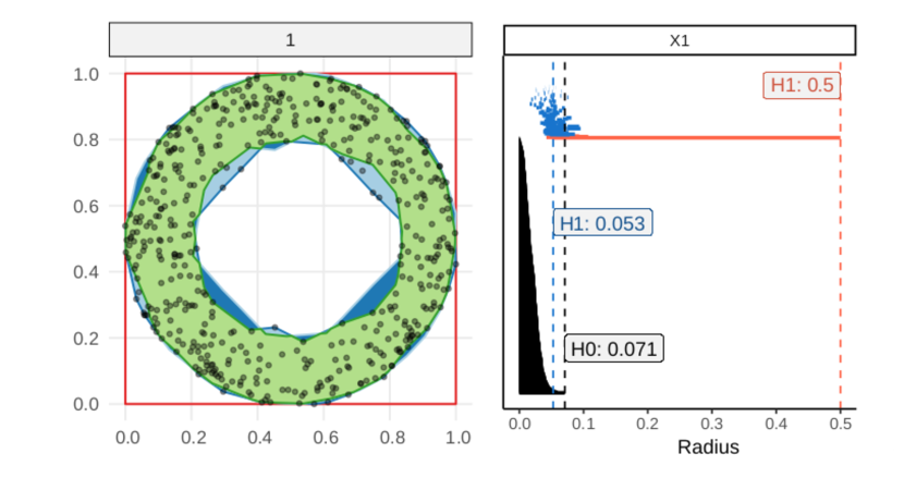
Figure 1 represents the barcodes for one set of data points arranged in a circle and having one hole in the middle (a doughnut). The central hole persists along multiple radius until it disappeared with $\varepsilon=0.5$. The long red line represent this feature persistence on $H_{1}$. The blue short lines are the noisy hole that appear and disappear briefly on the object. The black lines on the bottom are the number of connected components ($H_{0}$).

Figure 1: Manifold representing a circle with one hole and its corresponding barcode

2.4 Symmetries and Affine Geometry

Considering the Euclidean Plane $\mathbb{R}^{2}$, there are different geometries we can get by considering the action of different groups on it. Each group preserving a different set of properties that we would like to study. For example, for a point $p\in\mathbb{R}^{2}$, consider the action $\phi(p)=Ap+b$ where $A$ is a $2\times 2$ unitary matrix and $b\in\mathbb{R}^{2}$, this action preserves distance, a concept central to the Euclidian Geometry in a classical sense. Of course, the set of transformations described above is a group under composition and congruence is an invariant under the action of this set of transformations.

If we allow our set of transformations to be of the form $\phi(p)=Ap+b$ with $A$ an invertible matrix, then the geometry we get is more relaxed and the set of invariants of this action varies. This geometry is called Affine Geometry, and since not all invertible matrices are unitary, affine geometry does not leave congruence in the Euclidian sense as an invariant. Of course all isometries are affine transformations.

Since affine transformations preserve both parallelism and ratios along a given line, then it preserves ratios along parallel lines which implies that it preserves axial symmetry and that it carries within it other related properties in point sets.

In this study we will take advantage of this properties of affine geometry to talk about certain geometric qualities of point sets that are fundamental to understand sensitivity.

3 Methodology

In HernandezGeometrical2019 it is defined the way that the Vietoris Rips is constructed to determine the homological structure of the data. The method is based in the work of ZomorodianFast2010 on the use of cliques to dertermine the 2-simplex of the data.

In this work we determined a geometric correlation between the input and output variables. The algorithm allows us to measure the geometric pattern present in the data. The method consisted in three steps: 1. Build the Vietoris-Rips complex for a single given radius; 2. Estimate the bounding box contained inside the Vietoris-Rips complex; and 3. Compare the areas of the bounding box and the Vietoris-Rips complex to determine the percentage of blank space remained in the box.

The mentioned method is incapable to notice if one variable is relevant or not to the model. In other words, a variable with a non-noisy structure could be meaningless to explain the output. The behavior is explained as it does not matter what value takes the input variables, it does not get reflected over the output one. Even if there is some structural pattern, those values nullify each other to produce a non-influential process.

To explore further the intrinsic structure of the Vietoris-Rips complex, take the classic Ishigami model $f(X_{1},X_{2},X_{3})=\sin X_{1}+7\sin^{2}X_{2}+0.1X^{3}_{3}\sin X_{1}$ where $X_{d}\sim\text{Uniform}[-\pi,\pi]$ and $d=1,2,3$. The reader can find a complete discussion of this model in SaltelliScreening2009 .

Figure 2: The Ishigami model plot with $n=1000$ random points. Theoretically, $S_{1}=0.32$, $S_{2}=0.44$, $S_{3}=0$

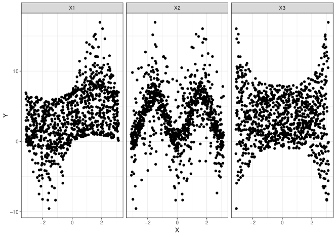
Notice from Figure 2 that the three variables have a clear pattern. The variable $X_{1}$ is increasing, variable $X_{2}$ has a M-shape and variable $X_{3}$ has bow-tie shape. In the three cases, HernandezGeometrical2019 estimated that the percentage of blank space is around 50%.

Nevertheless, the Sobol sensitivity indexes declare that the most important variable is $X_{2}$, followed by $X_{1}$ and finally $X_{3}$ has a theoretical null influence. One outstanding characteristic is how behaves the cloud of points around the line middle line $\overline{Y}=(\min{Y_{i}}+\max{Y_{i}})/2$. For the first two variables, we notice how the points upward the line does not produce the same pattern on the downwards sections. However, for the third variable $X_{3}$, both sections behave similar simulating a mirror effect.

Thus, to measure the mirror effect on a model, we propose the following procedure:

1. For each variable $X_{k}$, $k=1,\ldots,p$ and $Y$; project them in the $\mathbb{R}^{2}$ plane.

2. Estimate $(X_{\min},Y_{\min})=(\min\{X_{ki}\},\min\{Y_{i}\})$ for $i=1\ldots,n$.

3. Recenter all the points $\tilde{X}_{ki}=X_{ki}-X_{\min}$ and $\tilde{Y}_{ki}=Y_{i}-Y_{\min}$.

4. Create the Vietoris-Rips-complex $\mathcal{V}_{k}$ according to the procedure in HernandezGeometrical2019 for the cloud of points formed with $(\tilde{X}_{ki},\tilde{Y}_{i})$.

5. Create the symmetrical reflection $\mathcal{V}_{k}^{\text{SR}}$ of the Vietoris-Rips-complex and set it in the same plane of $\mathcal{V}_{k}$ (see Section 3.1).

6. Estimate the symmetric difference between both objects: $\mathcal{V}_{k}^{\triangle}=\mathcal{V}_{k}\triangle\mathcal{V}_{k}^{\text{SR}}$. Calculate the Area of $\mathcal{V}_{k}^{\triangle}$ and denote it as $\mathrm{Area}(\mathcal{V}_{\triangle})$. With those areas estimate the sensitivity index in Section 3.2,

   $$S_{i}^{\text{Geom}}=\frac{\mathrm{Area}(\mathcal{V}_{k}^{\triangle})}{2\ \mathrm{Area}(\mathcal{V}_{k})}$$

In the next sections we will describe in detail these steps.

3.1 Affine transformation of the Vietoris-Rips complex

Recall that the Vietoris-Rips-complex is the union of the i-th complexes for $i\in\{0,1,2,\ldots\}$ of a datapoint cloud. The 2-simplexes are formed with 3 vertex $(p_{k\alpha_{s}},p_{k\beta_{s}},p_{k\gamma_{s}})$ where the subindices $\alpha_{s}$, $\beta_{s}$ and $\gamma_{s}$ are permutations with repetitions from the sequence $1,\ldots,n$ and $s=1,\ldots,b_{2}$, where $b_{2}$ represents the second Betti number. Recall that each point has associated a pairwise coordinates, e.g., $p_{k\alpha_{i}}=(X_{k\alpha_{s}},Y_{\alpha_{s}})^{\top}$.

Define the affine transformation $\varphi(p)=Ap+b$ where

$$p =(x,y)^{\top}\in\mathbb{R}^{2}$$

$$A =\begin{pmatrix}1&0\\ 0&-1\end{pmatrix}$$

$$b =(0,2\ Y_{\operatorname{mid}})^{\top}$$

Applying the affine transformation $\varphi$ to each 2-simplex, we can create the Vietoris-Rips-complex reflection over the original one. However, this procedure fails if the data crosses the $x$-axis due to the reflection get distorted.

To remedy this, we first have to shift the datapoints to obtain a clear reflection through $\varphi$. To achieve this, recenter all the points to $\tilde{X}_{ki}=X_{ki}-X_{\min}$ and $\tilde{Y}_{ki}=Y_{i}-Y_{\min}$, this way all the data will be contained in the first quadrant.

To simplify the notation for the rest of the paper, we will assume that every datapoint has been shifted according the last paragraph.

Thus, for a single 2-simplex $[p_{1},p_{2},p_{3}]$ defined in Section 2.2 we can transform it applying the affine transformation explained in Section 2.4. Therefore, we have

$$\varphi([p_{1},p_{2},p_{3}])=\lambda_{1}\varphi(p_{1})+\lambda_{2}\varphi(p_{2})+\lambda_{3}\varphi(p_{3}).$$ (9)

where $\lambda_{1}+\lambda_{2}+\lambda_{3}=1$. Here we have abused of notation in $\varphi([p_{1},p_{2},p_{3}])$. It means, applying the transformation $\varphi$ to the whole 2-simplex $[p_{1},p_{2},p_{3}]$. By linearity, we apply $\varphi$ to inner point of $[p_{1},p_{2},p_{3}]$, therefore it turns into the right side of Equation (9).

Developing the last equation for a single point $p_{s}=(x_{s},y_{s})$ we have,

$$\varphi(p_{s}) =Ap_{s}+b$$

$$=\begin{pmatrix}1&0\\ 0&-1\end{pmatrix}\begin{pmatrix}x_{s}\\ y_{s}\end{pmatrix}+\begin{pmatrix}0\\ 2Y_{\operatorname{mid}}\end{pmatrix}$$

$$=\begin{pmatrix}x_{s}\\ 2Y_{\operatorname{mid}}-y_{s}\end{pmatrix}$$

Therefore, gathering this results for the three points in a 2-simplex $T$,

$$\varphi([p_{1},p_{2},p_{3}]) =\lambda_{1}\begin{pmatrix}x_{1}\\ 2\ Y_{\operatorname{mid}}-y_{1}\end{pmatrix}+\lambda_{2}\begin{pmatrix}x_{2}\\ 2\ Y_{\operatorname{mid}}-y_{2}\end{pmatrix}+\lambda_{3y}\begin{pmatrix}x_{3}\\ 2\ Y_{\operatorname{mid}}-y_{3}\end{pmatrix}$$

Finally, we define the symmetric reflection of $\mathcal{V}(G_{\varepsilon})$ as

$$\mathcal{V}_{k}^{\text{SR}}(G_{\varepsilon})=\varphi(\mathcal{V}_{k}(G_{\varepsilon}))=\bigcup_{s=1}^{b_{2}}\left\{\varphi([p_{k\alpha_{s}},p_{k\beta_{s}},p_{k\gamma_{s}}])\right\}$$

where $b_{2}$ represents the second Betti number.

Here we apply the affine transformation $\varphi$ to all the 2-simplex of the complex, and the join them into another complex.

For the rest of the paper, we will denote $\mathcal{V}_{k}\coloneqq\mathcal{V}_{k}(G_{\varepsilon})$ and $\mathcal{V}_{k}^{\text{SR}}\coloneqq\mathcal{V}_{k}^{\text{SR}}(G_{\varepsilon})$

3.2 Estimation of the geometrical sensitivity index

Once the symmetric reflection $\mathcal{V}_{k}^{\text{SR}}$ is estimated, we have to use it to determine if the variable $X_{k}$ is relevant or not. We mentioned before that one characteristic for the non-relevant variables is their symmetry through the $y$-middle axis. For this purpose, we will overlap the complexes $\mathcal{V}_{k}^{\text{SR}}$ with respect to $\mathcal{V}_{k}$ and gauge how much they are equal.

The symmetric difference between both complexes give the amount of area in either one but not in the intersection. We will denote the new set as

$$\mathcal{V}_{k}^{\triangle}=\left(\mathcal{V}_{k}\cup\mathcal{V}_{k}^{\text{SR}}\right)\setminus\left(\mathcal{V}_{k}\cap\mathcal{V}_{k}^{\text{SR}}\right).$$

Therefore, if the area of $\mathcal{V}_{k}^{\triangle}$ is small, it means that the union of original complex and the transformed one, is almost the same that their intersection. Otherwise, the points produced a particular pattern that the symmetric reflection cannot imitate. However, the complex $\mathcal{V}_{k}^{\text{SR}}$ replicate the same behavior of $\mathcal{V}_{k}$ in the opposite direction.

Once with the objects $\mathcal{V}_{k}$ and $\mathcal{V}_{k}^{\triangle}$ lets define the geometric sensitivity index as

$$S_{i}^{\text{Geom}}=\frac{\mathrm{Area}(\mathcal{V}_{k}^{\triangle})}{2\ \mathrm{Area}(\mathcal{V}_{k})}$$ (10)

The index $S_{i}^{\text{Geom}}$ measures how much the $\mathcal{V}_{k}$ and $\mathcal{V}^{\text{SR}}_{k}$ are asymmetrical.

We can identify two cases:

1. If $X_{k}$ is irrelevant to model $f$ (Equation (1)) a sensitivity index should be 0. The variable $X_{k}$ acts as a random input to the model causing a random pattern for the output.

   Here, we have that $\mathcal{V}_{k}$ and $\mathcal{V}^{\star}_{k}$ share the same structure (almost everywhere) due to the random interaction between $X_{k}$ and $Y$.

2. If $X_{k}$ is important to the model, thus its values cause a defined pattern to the output $Y$. Those patterns, in average, could be increasing, decreasing or a combination of both, for instance.

   In any case, the complexes $\mathcal{V}_{k}$ and $\mathcal{V}^{\star}_{k}$ have a non-negligible difference.

Considering these two cases, our index measures how asymmetrical are $\mathcal{V}_{k}$ and $\mathcal{V}^{\star}_{k}$ through the $\mathrm{Area}(\mathcal{V}_{k}^{\triangle})$. If the variable is irrelevant or random $\mathcal{V}_{k}\cong\mathcal{V}^{\star}_{k}$, which implies $\mathcal{V}_{k}^{\triangle}\cong\emptyset$. Therefore, the area of $\mathcal{V}_{k}^{\triangle}$ result in a negligible value.

In the other case, $\mathcal{V}_{k}\ncong\mathcal{V}^{\star}_{k}$. In the extreme case where the intersection of both sets are of measure zero, we have

$$\mathrm{Area}(\mathcal{V}_{k}^{\triangle})=\mathrm{Area}(\mathcal{V}_{k})+\mathrm{Area}(\mathcal{V}^{\star}_{k})=2\ \mathrm{Area}(\mathcal{V}_{k}).$$

Equation (10) summarizes both cases to get a index between 0 to 1.

4 Results

The methodology in this paper was compiled in a R (RCoreTeamLanguage2020 ) package called topsa: Topological Sensitivity Analysis (https://cran.r-project.org/package=topsa.

The additional packages used were TDA (FasyTDA2019 ) for estimating the Vietori-Rips structure, the package sf (PebesmaSimple2018 ) for all the geometric estimations and the package ggplot2 (WickhamGgplot22009 ) for all the graphic outputs.

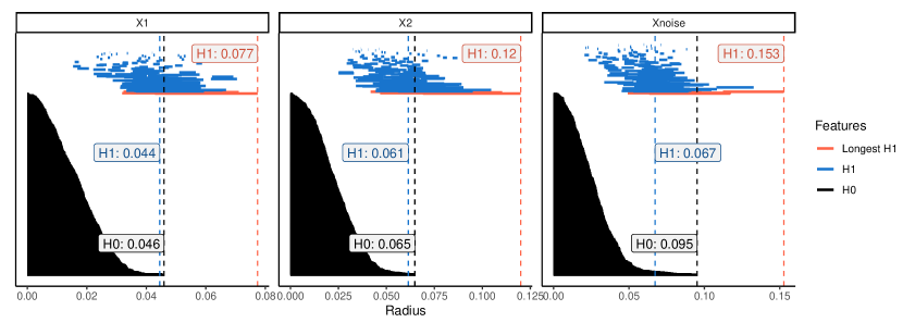
For all the settings, we sample $n=1000$ points with the distribution specified in each case. Due to the number of points, we choose the quantile $5\%$ for each case to determine the radius of the neighborhood graph. Further insights about this choosing will be presented in the conclusions section

We will consider five settings, each one with different topological features. The cases are not exhaustive and there are other settings with interesting features as well. However, through those examples we could show the capabilities of our models to detect sensitivity in each variable.

4.1 Theoretical examples

The examples considered are the following:

Linear

This is a simple setting with

$$Y=2X_{1}+X_{2}$$

and $X_{3}$ is an independent random variable. We set $X_{i}\sim\mathrm{Uniform}(-1,1)$ for $i=1,\ldots,3$.

Circle with hole:

The model in this case is

$$\begin{cases}X_{1}=r\cos(\theta)\\ Y=r\sin(\theta)\end{cases}$$

with $\theta\sim\mathrm{Uniform}(0,2\pi)$ and $r\sim\mathrm{Uniform}(0.5,1)$. This form creates a circle with a hole in the middle.

Connected circles with holes:

The model consists in three different circles, where we set $\theta\sim\mathrm{Uniform}(0,2\pi)$:

1. Circle centered at $(0,0)$ with radius between 1.5 and 2.5:

   $$\begin{cases}X_{1}=r_{1}\cos(\theta)\\ Y=r_{1}\sin(\theta)\end{cases}$$

   where $r_{1}\sim\mathrm{Uniform}(1.5,2.5)$.

2. Circle centered at $(3.5,3.5)$ with radius between 0.5 and 1:

   $$\begin{cases}X_{2}-3.5=r_{2}\cos(\theta)\\ Y-3.5=r_{2}\sin(\theta)\end{cases}$$

   where $r_{2}\sim\mathrm{Uniform}(0.5,1)$.

3. Circle centered at $(-4,4)$ with radius between 1 and 2:

   $$\begin{cases}X_{3}+4=r_{3}\cos(\theta)\\ Y-4=r_{3}\sin(\theta)\end{cases}$$

   where $r_{3}\sim\mathrm{Uniform}(1,2)$.

Ishigami:

The final model is

$$Y=\sin X_{1}+7\ \sin^{2}X_{2}+0.1\ X_{3}^{4}\sin X_{1}$$

where $X_{i}\sim\mathrm{Uniform}(-\pi,\pi)$ for $i=1,2,3$, $a=7$ and $b=0.1$.

4.2 Numerical results

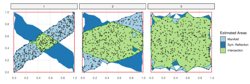
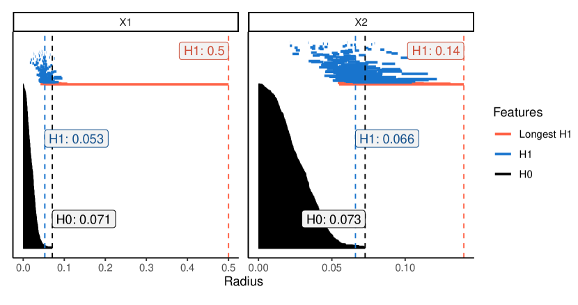
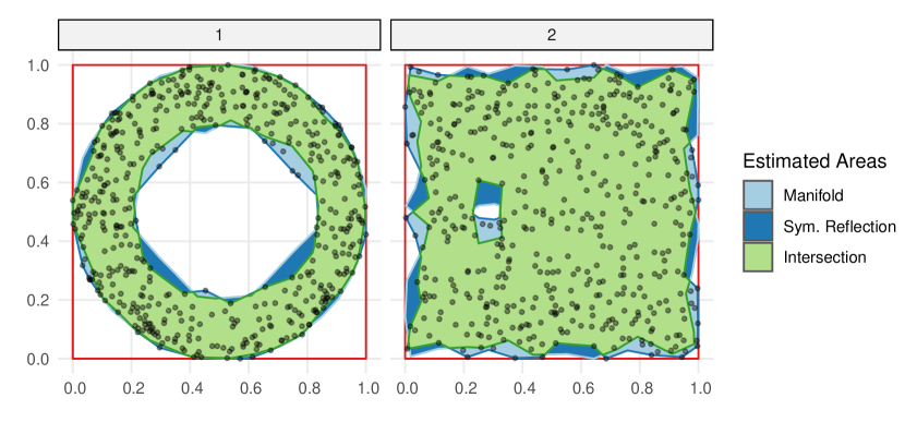
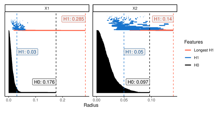
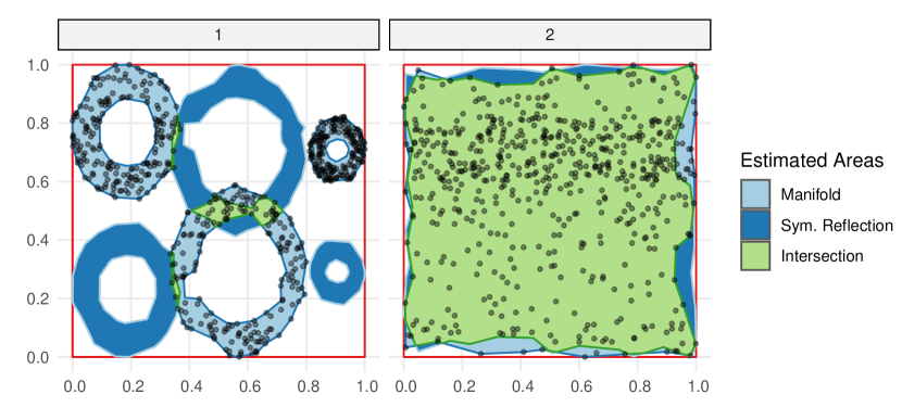
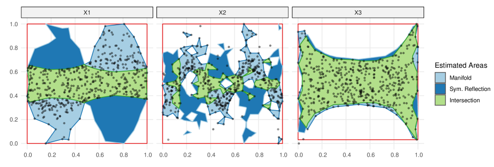
The results in this section were estimated with the code topsa. The figures are estimated Vietoris-Rips-complex for each input $X_{i}$ with respect to the output variable $Y$. Also, we represent the symmetric reflection of this complex and the symmetric difference between them. The table below each figure presents the radius used to build the neighborhood graph, the estimated areas of the manifold object ($\mathrm{Area}(\mathcal{V})$), the area of the reference box contained the complex ($\mathrm{Area}(B)$), the geometrical correlation index estimated in HernandezGeometrical2019 ($\rho^{\mathrm{Geom}}$), and the geometric sensitivity index ($S^{\mathrm{Geom}}$).

The linear model in Figure 3 allow us to identify that the variable $X_{1}$ doubles the relevance of $X_{2}$. The indices $\rho^{\mathrm{Geom}}$ and $S^{\mathrm{Geom}}$ are coherent in this case. The variables $X_{3}$ to $X_{5}$ will have less relevant indices. We conclude how the empty spaces are present according to the relevance level of the variable.

Variable	$\varepsilon$	$\mathrm{Area}(\mathcal{V}(G))$	$\mathrm{Area}(B)$	$S_{i}^{\mathrm{Geom}}$	$S_{i}$
$X_{1}$	0.08	0.31	1.00	0.69	0.81
$X_{2}$	0.12	0.64	1.00	0.36	0.19
$X_{3}$	0.15	0.80	0.98	0.19	0.01

Figure 3: Results for the Linear case.

The model of a circle with a hole in Figure 4 presents a topological particularity. It is a model were there exist a clear geometric pattern between $X_{1}$ and $Y$ but neither $X_{1}$ nor $X_{2}$ are relevant. Observe how the first variable has $\rho_{1}^{\mathrm{Geom}}$ equal to $0.48$ and the $\rho_{2}^{\mathrm{Geom}}$ equals to $0.08$. However, $S_{1}^{\mathrm{Geom}}$ and $S_{2}^{\mathrm{Geom}}$ are less than $0.05$. It means, our estimators detect a geometrical correlation in the first variable but neither one has impact in the model.

Variable	$\varepsilon$	$\mathrm{Area}(\mathcal{V}(G))$	$\mathrm{Area}(B)$	$S_{i}^{\mathrm{Geom}}$	$S_{i}$
$X_{1}$	0.10	2.07	3.94	0.48	0.03
$X_{2}$	0.13	3.66	3.99	0.08	0.04

Figure 4: Results for the Circle with hole case.

The other atypical case is a model of connected circles with holes in Figure 5. Both circles have different scales and positions. In this case, the first variable has a geometric pattern while the second one is random input. Both the $\rho^{\mathrm{Geom}}$ and $S^{\mathrm{Geom}}$ detect that the first variable is the geometric relevant while the second not.

Variable	$\varepsilon$	$\mathrm{Area}(\mathcal{V}(G))$	$\mathrm{Area}(B)$	$S_{i}^{\mathrm{Geom}}$	$S_{i}$
$X_{1}$	0.09	0.23	1.00	0.77	0.64
$X_{2}$	0.16	0.92	1.00	0.08	0.01

Figure 5: Results for the Circle with two hole case.

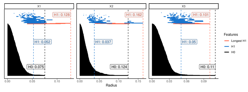
Another classic model is the Ishigami. model in sensitivity analysis because it presents a strong non-linearity and non-monotonicity with interactions in $X_{3}$. With other sensitivity estimators the variables $X_{1}$ and $X_{2}$ have great relevance to the model, while the third one $X_{3}$ has almost zero. For a further explanation of this function we refer the reader to SobolUse1999 . Figure 6. In our case all the geometric correlations are between 0.5 to 0.7. As noticed by HernandezGeometrical2019 , this measure detects the geometric structure present in every variable. But, this measure gives an incomplete perspective of the problem because is not saying if they are relevant or not to the model. For this, the index $S^{\mathrm{Geom}}$ establish the order of relevance of the variables as: $X_{2},X_{1},X_{3}$. This match with the theoretical case discussed at the beginning of Section 3.

Variable	$\varepsilon$	$\mathrm{Area}(\mathcal{V}(G))$	$\mathrm{Area}(B)$	$S_{i}^{\mathrm{Geom}}$	$S_{i}$
$X_{1}$	0.16	0.48	1.00	0.49	0.29
$X_{2}$	0.08	0.27	1.00	0.64	0.48
$X_{3}$	0.13	0.49	0.97	0.07	0.02

Figure 6: Results for the Ishigami case.

5 Conclusions

In this work we proposed a simple method to detect the relevance of a variable in a model. We estimated first the embedding manifold in $\mathbb{R}^{2}$ of each input variable and the output variable $Y$. We use the Vietoris-Rips as a proxy for the intrinsic geometry of the object. By application of simple affine transformations we compared the area of the estimated manifold to that of its symmetric reflection and use this information to create a score. If their symmetric difference were small in terms of area relative to the whole geometric pattern, the variable’s relevance were small as well. Otherwise it would be higher.

As our experiments show, the geometric sensitivity index constructed in our method detected the geometric structure within the point cloud. Even if the construction depends on the simplicial complexes, we based the method on the area of the complex. This simplified the understanding of the index for non-technical users. Our index calculated the empty space created by the data after re-scaling to the the interval $[0,1]\times[0,1]$. This approach allowed us to normalize the total space taken by the data. If the space is small, then there is not an obvious pattern between the variable and their response. Otherwise, we can recognize patterns that influenced the value of $Y$.

One caveat of this method was the choice of radius in order to construct the Vietoris-Rips complex. This parameter is the most sensible part of the method, and yet the most difficult to select. In our examples, we first observed the barcode and selected the radius according to the most prominent features on the data. An automated approach to this selection can be done and can be implemented as part of the algorithm.

While the method provided here showed to be of use, we recognize that its extension into higher dimension modeling and for the analysis of multiple variables at a time can be very costly in a computational sense. Another issue would be to determine the hyperspace symmetrization and the subsequent calculation of hyper volumes. One plausible approach to solving this problem would either be projecting the data in low dimensional spaces by means of principal component analysis, projection pursuit or following an specific direction in a grand tour (CookGrand2008 ).

Other natural approach to extend this method to a broader class of problems will follow by exploiting the deeper topological features of the data. Tools like Euler curves, landscapes or cohomology analysis would presumably lead to new insights on the relevance of each variable in the model.

Declarations

Funding

First and second authors acknowledge the financial support from Escuela de Matemática de la Universidad de Costa Rica, through CIMPA, Centro de Investigaciones en Matemática Pura y Aplicada through the projects 821–B7–254 and 821–B8–221 respectively.

Third author acknowledges the financial support from Escuela de Matemática de la Universidad de Costa Rica, through CIMM, Centro de Investigaciones Matemáticas y Metamatemáticas through the project 820–B8–224.

Code availability

All the calculations in this package were made using an own R-package topsa. It estimates sensitivity indices reconstructing the embedding manifold of the data. The reconstruction is done via a Vietoris Rips with a fixed radius. Then the homology of order 2 and the indices are estimated. The package is published on CRAN on this address https://cran.r-project.org/package=topsa

Conflict of interests

On behalf of all authors, the corresponding author states that there is no conflict of interest.

References

- [1] Nieves Atienza, Rocio Gonzalez-Diaz, Enlace a sitio externo Este enlace se abrirá en una ventana nueva, and Matteo Rucco. Persistent entropy for separating topological features from noise in vietoris-rips complexes. Journal of Intelligent Information Systems; New York, 52(3):637–655, 2019.
- [2] Peter Bubenik. Statistical topological data analysis using persistence landscapes. arXiv:1207.6437 [cs, math, stat], January 2015.
- [3] Francesca Campolongo, Andrea Saltelli, and Jessica Cariboni. From screening to quantitative sensitivity analysis. A unified approach. Computer Physics Communications, 182(4):978–988, April 2011.
- [4] Frédéric Chazal, Leonidas J. Guibas, Steve Y. Oudot, and Primoz Skraba. Persistence-Based Clustering in Riemannian Manifolds. Journal of the ACM, 60(6):41:1–41:38, November 2013.
- [5] David Cohen-Steiner, Herbert Edelsbrunner, and John Harer. Stability of Persistence Diagrams. Discrete & Computational Geometry, 37(1):103–120, January 2007.
- [6] Anne Collins, Afra Zomorodian, Gunnar Carlsson, and Leonidas J. Guibas. A barcode shape descriptor for curve point cloud data. Computers & Graphics, 28(6):881–894, December 2004.
- [7] Benoit Combes, Robin Hennessy, John Waddington, Neil Roberts, and Sylvain Prima. Automatic symmetry plane estimation of bilateral objects in point clouds. In 2008 IEEE Conference on Computer Vision and Pattern Recognition, pages 1–8, June 2008.
- [8] Dianne Cook, Andreas Buja, Eun-Kyung Lee, and Hadley Wickham. Grand Tours, Projection Pursuit Guided Tours, and Manual Controls. In Chun-houh Chen, Wolfgang Härdle, and Antony Unwin, editors, Handbook of Data Visualization, Springer Handbooks Comp.Statistics, pages 295–314. Springer, Berlin, Heidelberg, 2008.
- [9] Vin de Silva and Robert Ghrist. Coverage in sensor networks via persistent homology. Algebraic \& Geometric Topology, 7(1):339–358, April 2007.
- [10] Brittany T. Fasy, Jisu Kim, Fabrizio Lecci, Clement Maria, David L. Millman, and Vincent Rouvreau Maria. TDA: Statistical Tools for Topological Data Analysis, December 2019.
- [11] Robert Ghrist. Barcodes: The persistent topology of data. Bulletin of the American Mathematical Society, 45(1):61–75, October 2008.
- [12] Loïc Le Gratiet, Stefano Marelli, and Bruno Sudret. Metamodel-Based Sensitivity Analysis: Polynomial Chaos Expansions and Gaussian Processes. In Roger Ghanem, David Higdon, and Houman Owhadi, editors, Handbook of Uncertainty Quantification, pages 1–37. Springer International Publishing, Cham, 2015.
- [13] Allen Hatcher. Algebraic Topology. Cambridge Univ. Press, Cambridge, 2000.
- [14] Alberto Hernández, Maikol Solís, and Ronald Zúñiga. Geometrical correlation indices using homological constructions on manifolds. Manuscript submitted for publication, 2019.
- [15] T. Ishigami and Toshimitsu Homma. An importance quantification technique in uncertainty analysis for computer models. In Uncertainty Modeling and Analysis, 1990. Proceedings., First International Symposium On, pages 398–403. IEEE, 1990.
- [16] Max Z. Li, Megan S. Ryerson, and Hamsa Balakrishnan. Topological data analysis for aviation applications. Transportation Research Part E: Logistics and Transportation Review, 128:149–174, August 2019.
- [17] Rajendra Nagar and Shanmuganathan Raman. Detecting Approximate Reflection Symmetry in a Point Set Using Optimization on Manifold. IEEE Transactions on Signal Processing, 67(6):1582–1595, March 2019.
- [18] Nina Otter, Mason A. Porter, Ulrike Tillmann, Peter Grindrod, and Heather A. Harrington. A roadmap for the computation of persistent homology. EPJ Data Science, 6(1):17, December 2017.
- [19] Eduardo Paluzo-Hidalgo, Rocio Gonzalez-Diaz, and Miguel A. Gutiérrez-Naranjo. Towards a Philological Metric through a Topological Data Analysis Approach. arXiv:1912.09253 [cs, math], January 2020.
- [20] Edzer Pebesma. Simple Features for R: Standardized Support for Spatial Vector Data. The R Journal, 10(1):439, 2018.
- [21] R Core Team. R: A Language and Environment for Statistical Computing, 2020.
- [22] Erik Rybakken, Nils Baas, and Benjamin Dunn. Decoding of Neural Data Using Cohomological Feature Extraction. Neural Computation, 31(1):68–93, January 2019.
- [23] Andrea Saltelli, Paola Annoni, Ivano Azzini, Francesca Campolongo, Marco Ratto, and Stefano Tarantola. Variance based sensitivity analysis of model output. Design and estimator for the total sensitivity index. Computer Physics Communications, 181(2):259–270, February 2010.
- [24] Andrea Saltelli, Francesca Campolongo, and Jessica Cariboni. Screening important inputs in models with strong interaction properties. Reliability Engineering & System Safety, 94(7):1149–1155, July 2009.
- [25] I. M. Sobol and Yu.L. Levitan. On the use of variance reducing multipliers in Monte Carlo computations of a global sensitivity index. Computer Physics Communications, 117(1-2):52–61, March 1999.
- [26] I.M. Sobol. Sensitivity Estimates for Nonlinear Mathematical Models. Mathematical Modeling and Computational experiment, 1(4):407–414, 1993.
- [27] I.M. Sobol, S. Tarantola, D. Gatelli, S.S. Kucherenko, and W. Mauntz. Estimating the approximation error when fixing unessential factors in global sensitivity analysis. Reliability Engineering & System Safety, 92(7):957–960, July 2007.
- [28] Maikol Solís. Non-parametric estimation of the first-order Sobol indices with bootstrap bandwidth. Communications in Statistics - Simulation and Computation, pages 1–16, August 2019.
- [29] Bernadette J. Stolz, Heather A. Harrington, and Mason A. Porter. Persistent homology of time-dependent functional networks constructed from coupled time series. Chaos: An Interdisciplinary Journal of Nonlinear Science, 27(4):047410, April 2017.
- [30] Hadley Wickham. Ggplot2: Elegant Graphics for Data Analysis. Use R! Springer-Verlag, New York, 2009.
- [31] Afra Zomorodian. Fast construction of the Vietoris-Rips complex. Computers \& Graphics, 34(3):263–271, June 2010.
- [32] Afra Zomorodian and Gunnar Carlsson. Computing persistent homology. Discrete and Computational Geometry, 2005.