Towards a Probabilistic Foundation of Relativistic Quantum Theory:
The One-Body Born Rule in Curved Spacetime

Abstract

In this work we establish a novel approach to the foundations of relativistic quantum theory, which is based on generalizing the quantum-mechanical Born rule for determining particle position probabilities to curved spacetime. A principal motivator for this research has been to overcome internal mathematical problems of quantum field theory (QFT) such as the ‘problem of infinities’ (renormalization), which axiomatic approaches to QFT have shown to be not only of mathematical but also of conceptual nature. The approach presented here is statistical by construction, can accommodate a wide array of dynamical models, does not rely on the symmetries of Minkowski spacetime, and respects the general principle of relativity.

In the analytical part of this work we consider the $1$-body case under the assumption of smoothness of the mathematical quantities involved. This is identified as a special case of the theory of the general-relativistic continuity equation. While related approaches to the relativistic generalization of the Born rule assume the hypersurfaces of interest to be spacelike and the spacetime to be globally hyperbolic, we employ prior contributions by C. Eckart and J. Ehlers to show that the former condition is naturally replaced by a ‘non-tangency condition’ and that the latter one is obsolete. We discuss two distinct formulations of the $1$-body case, which, borrowing terminology from the non-relativistic analog, we term the Lagrangian and Eulerian pictures. We provide a comprehensive treatment of both. The main contribution of this work to the mathematical physics literature is the development of the Lagrangian picture. The Langrangian picture shows how one can resolve the ‘problem of time’ in this approach and therefore serves as a blueprint for the generalization to many bodies and the case that the number of bodies is not conserved.

We also provide an example to illustrate how this approach can in principle be employed to model particle creation and annihilation.

Keywords:
Relativistic conservation laws   -   Relativistic quantum mechanics
Axiomatic quantum field theory   -   Problem of time
Dirac equation   -   Flowout   -   Beyond the Standard Model
MSC2020:
81T20   -   81T99   -   81P99   -   83C47   -   83C40

1 Introduction

Since this work is addressed to both mathematical physicists and mathematicians and the reader might not have a strong background in theoretical particle physics, we begin with a general historical motivation in Sec. 1.1. In Sec. 1.2 we argue why it is the (general-)relativistic generalization of the Born rule that provides a natural approach to the foundations of relativistic quantum theory. Respective analytical results on the one-body theory, which constitute the core contribution of this work, are summarized in Sec. 1.3. In Sec. 1.4 we provide some remarks on the directly related literature. Notations and conventions are given in Sec. 1.5.

Readers only interested in our analytical results are invited to skip to Secs. 1.3 and 1.5.

1.1 Historical background and motivation

The Standard Model of Particle Physics (SM) is contemporarily the empirically most successful theory of the fundamental constituents of matter and its mutual interactions. While it does not incorporate the gravitational interaction, in its ability to provide such a unified description lies arguably its greatest achievement.

The theoretical framework that underlies the SM is known as relativistic quantum field theory (QFT). Historically, the abstract framework of QFT emerged out of perturbative descriptions of physical phenomena involving electrons and electromagnetic radiation: quantum electrodynamics (QED) in its early stages. First articles on the topic appeared in the late 1920s and early 1930s [113]. In order to attain a physically acceptable theory of radiation that is also able to describe quantum phenomena of matter, one ultimately had to generalize the non-relativistic theory of quantum mechanics (QM) to the (special-)relativistic setting. In this generalization lies the theoretical justification for the existence of QFT (cf. p. xi in Ref. [201]).

From the 1930s up until the late 1940s QED was, however, generally viewed with great skepticism. This was mostly due to the appearance of unphysical divergences in the theory, the so called ‘problem of infinities’ (cf. Sec. 1.3 in Ref. [201], Ref. [113], Sec. 5 in Ref. [33], and Ref. [168]). It was the perceived failure of the $1$-electron Dirac theory [42] to account for a variety of spectroscopic measurements [141, 116, 142, 115, 63], that created the need for an alternative approach. Bethe’s and other theoreticians’ success in accounting for those experimental anomalies within QED enabled the theory to meet this demand. While their method of ‘renormalizing’ the charge and mass of the electron was ad hoc, mathematically unsound, and it did not entirely resolve ‘the problem of infinites’ [47, 64], the lack of empirically viable competition meant that QED was to emerge victoriously.

Moreover, the success of QED in this question was going to determine subsequent developments in theoretical particle physics. QFT became the language of the field moving forward, thus ingraining the idea of renormalization. Despite overt mathematical problems of the formalism, over the coming decades QFT proved itself to be sufficiently flexible to accommodate and sometimes even predict new experimental data. Undoubtedly, it was also the close collaboration between theoreticians and experimentalists during that time that eventually enabled QFT to serve as the theoretical foundation for the SM we employ today.

While the SM represents a significant milestone in the history of particle physics, there is a growing concern with regards to the problem that the vast majority of so called ‘Beyond the Standard Model’ research has provided few, if any, empirically tangible results [183, 206, 96, 97]. In this respect, it is worth noting that in the history of science it is not uncommon for a subject area to pass through such a phase of apparent stagnation. Overcoming it in a scientifically fruitful manner usually necessitates a careful reevaluation of underlying methodologies and assumptions. Although this process is commonly resisted by practitioners in the subject, it is nonetheless necessary for its scientific integrity (cf. Refs. [114, 150]).

In order to address at least some of the internal mathematical problems of QFT, mathematical physicists began the process of crafting it into a rigorous formalism in the early 1950s. Starting with works by Friedrichs [69, 73, 70, 71, 72], Wightman [203, 204], Cook [34] and others [122, 173, 106, 4], this methodological shift eventually gave rise to a variety of research programs and axiomatic systems: the most well-known ones are ‘axiomatic quantum field theory’ (the Wightman axioms; cf. Ref. [204] and Sec. 3.1 in Ref. [184]), ‘algebraic quantum field theory’ (the Haag-Kastler axioms; cf. Refs. [81, 80]), and ‘constructive quantum field theory’ (the Osterwalder-Schrader axioms and extensions by Glimm and Jaffe; cf. Refs. [148, 149, 78]). Though axiomatic approaches to QFT were at times being criticized for their limited practical applicability (cf. Sec. II in Ref. [29]), today their scientific value has become generally acknowledged. Axiomatic approaches to QFT have contributed to particle physics by clarifying both the concepts and mathematical structures employed in ‘perturbative QFT’ [64].

While axiomatic approaches to QFT constitute an important methodological step in the history of theoretical particle physics, we wish to articulate the following objection to purely formal approaches to resolving the difficulties of perturbative QFT: The search for an axiomatic foundation for the subject is necessarily accompanied by an identification of its basic concepts and how those relate to the natural phenomena one intends to explain. Especially with regards to the concept of renormalization, it is worthwhile to remember that the goal is not to reproduce what is known to be inconsistent. Rather, it is to construct an internally consistent relativistic quantum theory that can compete with the empirical successes of the SM.

Achieving this goal may require a revision of the basic concepts of contemporary relativistic quantum theory. Although this may seem like a bold task at first, one may find hope in recalling that QFT is merely the language in which developments of the field have historically been formulated [110]—a language that is still questionable on logical grounds. To acknowledge the need to change this language does not necessarily translate to ‘throwing out the baby with the bathwater’. It merely means acknowledging the need for a different theoretical perspective on existing results.

Providing such a perspective is indeed the primary aim of this work and the research program it is intended to give rise to.

1.2 The Born rule as a novel approach to relativistic quantum theory

The approach suggested and pursued in this work is based on the Born rule in (non-relativistic) QM.

Following Pauli’s original formulation, the rule determines the probability that the positions of one or several particles lie in a given ‘region’ of configuration space at fixed time. More precisely, if $\rho(t,\vec{x}_{1},\dots,\vec{x}_{N})$ denotes the values of the (time-dependent) probability density $\rho$ at time $t\in\mathbb{R}$ and at points $(\vec{x}_{1},\dots,\vec{x}_{N})\in\mathbb{R}^{3N}$, as obtained from a respective (normalized) $N$-body Schrödinger [175] or Pauli [152] wave function, then

$$\mathbb{P}_{t}(U)=\int_{U}\rho(t,\vec{x}_{1},\dots,\vec{x}_{N})\,\mathrm{d}^{3}x_{1}\dots\mathrm{d}^{3}x_{N}$$ (1.1)

gives the probability that at time $t$ the bodies are positioned within a (Lebesgue) subset $U$ in $\mathbb{R}^{3N}$.

For the purpose of constructing a relativistic quantum theory, there are two major reasons why one would focus on this particular aspect of the non-relativistic theory:

First, as opposed to vectors in an abstract Hilbert space or even elements of the Fock space constructed thereof, the Born rule is formulated directly in terms of spatio-temporal concepts. One may therefore expect there to be a more or less straightforward generalization to the relativistic setting.

Second, the Born rule is fundamentally a statistical statement: Taking its generalization as a point of departure for the relativistic theory guarantees that the latter is of statistical nature from the onset.

Evidently, this will also tie the particle concept into the basic structure of the theory. Yet this is should not come as a surprise, since the particle concept is central to the non-relativistic theory and any straightforward relativistic generalization will therefore inherit it.^,

In their 1929 article [88], which was foundational to the development of quantum field theory, Heisenberg and Pauli did indeed consider a particle-based approach. They chose to reject it on the following grounds:

As is generally known, in classical point mechanics a relativistically invariant formulation of the many-body problem with the aid of the Hamiltonian theory is not feasible. One may therefore not hope that in the quantum theory a relativistically invariant treatment of the many-body problems with differential equations in configuration space […] will be attainable […]

[translated from German]

Heisenberg and Pauli did thus not consider the notion that a particle-based relativistic quantum theory could be constructed which does not rely on ‘quantizing’ a ‘classical’ Hamiltonian system.

This is the point at which this work parts ways with their reasoning.

Rest assured, we do not deny that there may be physical situations in which the concept of a discrete particle ceases to be a viable physical concept and a field description becomes more appropriate. Yet due to the centrality of the particle concept to QM and its non-relativistic siblings (see e.g. Refs. [160, 163, 144, 44]), such situations are beyond the purview of a mere relativistic generalization of those theories. The conservative approach is therefore to put the particle concept at the center of such a generalization—as Heisenberg and Pauli implicitly admitted with their above statement.

Still, the historical context justifies the assertion that the construction of a relativistic quantum theory with the particle concept at its center has shown itself to be a difficult problem.

In particular, if one does take the generalization of the Born rule as an approach to the problem, there are two major hurdles one needs to address:

1. The so called ‘problem of time’: On the one hand, Eq. (1.1) above indirectly refers to the different spatial positions of the bodies at the same instance of time. On the other hand, in the theory of relativity the notion of simultaneity lacks the physical significance it has in non-relativistic theories.

   In special relativity this is known to be a consequence of the special principle of relativity in conjunction with the invariance of the speed of light (in vacuum). In the general theory of relativity it may be considered a consequence of the general principle of relativity. Einstein [56] phrased the latter as follows:

   We shall be true to the principle of relativity in its broadest sense if we give such a form to the laws that they are valid in every such four-dimensional system of co-ordinates, that is, if the equations expressing the laws are co-variant with respect to arbitrary transformations.

   If understood in a broad sense, the general principle of relativity also demands that we may not employ any quantities in the formulation of fundamental physical laws that depend on a particular choice of physical observer, frame of reference, ‘initial’ hypersurface, etc.

   A priori, there is thus reasonable doubt as to whether a relativistic generalization of the Born rule can be made sense of. It is indeed a matter of simple counting that in an $(n+1)$-dimensional spacetime $\mathcal{Q}$ with $N$ bodies ($n,N\in\mathbb{N}$) the most obvious candidate for a ‘relativistic configuration space’, the $N$-fold product manifold $\mathcal{Q}^{N}$, is $N(n+1)$-dimensional—so that there are $N-1$ ‘too many time dimensions’.

2. The problem of dynamics: For Eq. (1.1) to define a probability measure at each $t\in\mathbb{R}$, the probability conservation law $\mathbb{P}_{t}(\mathbb{R}^{3N})\equiv 1$ needs to hold. In non-relativistic QM this is assured by the fact that the time evolution operator $U_{t}=\exp(-\mathfrak{i}t\hat{H}/\hbar)$ is unitary for each $t$ whenever the given Hamiltonian $\hat{H}$ is self-adjoint. This, in turn, suggests that for the relativistic theory we need to introduce a (possibly indirect) assertion on how the time evolution is modeled. Yet this makes it difficult to fully separate the probabilistic and the dynamical aspects of the theory.

   Historically, the conceptual problems with viewing the Dirac equation as a $1$-body evolution equation were indeed one of the main motivators for pursuing the development of quantum field theory over a deeper understanding of relativistic $N$-body theories.

There are two main works in the recent literature that propose a relativistic generalization of the Born rule:

In Ref. [124] Lienert and Tumulka suggest a construction for $N$ bodies in Minkowski spacetime which takes the configuration space to be the $N$-fold product of a Cauchy surface therein. In this work an ‘instant of time’ is viewed as a choice of Cauchy surface. Different Hilbert spaces are associated with the respective hypersurfaces and the existence of a unitary time-evolution operator between the two surfaces is postulated, in analogy to the Schrödinger picture of QM. The authors do not commit to any particular dynamical models, though the considered examples were all descendants of the ($1$-body) Dirac equation (cf. Sec. 4 in Ref. [124]). For the many-body case the considered models seem to lack physical justification, with the exception of “free Dirac evolution”.

Contrarily, Miller et al. [136] consider the more general case of a globally hyperbolic spacetime and then use Bernal and Sanchez’ stronger version [12, 13] of Geroch’s Splitting Theorem [77] to construct an ‘$N$-particle configuration spacetime’. The latter is chosen to be the product of $\mathbb{R}$ with the $N$-fold product of a Cauchy surface (cf. Sec. 2.2 in Ref. [136]). The authors were indeed able to prove an invariance theorem to address the ‘problem of time’ (cf. Thm. 22.(ii) in Ref. [136] as well as Thm. 2 in Ref. [135]). Yet the proposed dynamical equations violate the general principle of relativity (cf. Eqs. 20 and 24 in Ref. [136]).

In this work we develop the theory of the $1$-body Born rule on curved spacetime under the assumption of smoothness of the mathematical quantities involved. This novel generalization mainly draws from prior contributions to the theory of general-relativistic fluid mechanics due to Eckart [50] and Ehlers [54]. We show that there are two distinct formulations of the theory for the case that one allows for the temporal evolution of the quantities involved. In full analogy to the non-relativistic analog, we term those formulations the Lagrangian picture and the Eulerian picture, respectively.

The development of the Lagrangian picture we view as the main contribution of this work to the foundations of relativistic quantum theory: The construction of the Lagrangian picture for the $1$-body case opens up a potentially viable path towards the generalization of the theory to the $N$-body case or even the case that the number of bodies is not conserved.

Like Miller et al. [135, 136], we address the ‘problem of time’ in this formulation by proving an invariance property that assures that the general principle of relativity is indeed respected (cf. Thm. 3.1.4 and 3.1.4).

While we do not suggest any explicit dynamical models, we show in several examples how the Dirac equation fits into the formalism. The structural aspects of the theory are the focus of this work. We thereby provide a mathematical framework that is in principle agnostic with respect to the dynamics one wishes to impose—be it through a relativistic wave equation or other (possibly non-linear) partial differential equations for the respective fundamental quantities of the theory.

The general idea that the probabilistic and the dynamical aspects of relativistic quantum theory may be treated separately is inspired by the non-relativistic Madelung equations [127, 128] and their close connection to Kolmogorov’s theory of probability (cf. Chap. 2 in Ref. [161]). Though their precise mathematical relation to the Schrödinger equation is still a subject of mathematical research [198, 197, 199, 75, 160, 31, 132, 163], the Madelung equations allow one to separate the equation of continuity from ‘the dynamics’, as encoded by an equation containing the forces/potentials.

In the relativistic theory one is thus not bound to the difficult task of guessing appropriate wave equations that have to make sense in a statistical context—as Dirac was miraculously able to do [42, 37].

The reason that we have pursued a generalization of the Born rule to the general-relativistic setting, as opposed to being satisfied with a special-relativistic version, is that this approach is not only more general but simpler: As Hollands and Wald have noted on p. 87 sq. of their article [93], Minkowski spacetime constitutes a highly symmetrical setting, yet even a special-relativistic quantum theory ought not to rely on those symmetries in its basic formulation. From a mathematical perspective those symmetries constitute ‘obsolete assumptions’, thus making a construction of the theory on curved spacetime the natural approach. Of course, for practical purposes and at this point in time, one is nonetheless primarily interested in how the theory works in Minkowski spacetime.

Finally, we wish to point out that the theory we develop in this work is most easily understood from the point of view of the statistical/ensemble interpretation of QM. In essence, this interpretation states that the primary utility of QM is to make statistical predictions on the ‘physical observables’ of ‘similarly prepared systems’ of particles—that is the ensemble obtained by taking the collection of all (uncountably many) ‘samples’. While one would be justified to view this as a ‘minimalist’ interpretation of QM, there does exist an implicit conflict with the Copenhagen interpretation insofar as statements such as “the electron is in state $\Psi$” become meaningless—the words ‘state’ and ‘quantum system’ always refer to an ensemble of individual physical systems, not the systems themselves. The interested reader is referred to Refs. [6], [153], and Sec. 2.1 in Ref. [161] for a general introduction to the subject.

Ultimately and as explained in Sec. 1.1 above, the mathematical axiomatization of relativistic quantum theory requires an identification of its basic concepts. It is in this sense that the progress that was achieved in the foundations of QM via the development of the ensemble interpretation has a direct bearing on the theory we develop here. Yet since the work is primarily of mathematical nature, we use the ensemble interpretation mostly for methodological purposes (cf. [181]). The reader is, of course, free to choose their own interpretation. Still, how one resolves the fundamental questions of the non-relativistic theory is bound to lead to different judgments on whether one deems a particular approach to the relativistic theory as reasonable or not. That is, the ongoing debate on the conceptual foundations of quantum mechanics [101, 102, 66, 67] cannot be fully separated from the discussion of the mathematical foundations of relativistic quantum theory.

1.3 Summary of analytical results and outlook

The central contribution of this work is the comprehensive development of the theory of the $1$-body Born rule on curved spacetime under the assumption of smoothness of the mathematical quantities involved.

From a mathematical perspective, this theory may be viewed as a special case of the theory of the general-relativistic continuity equation. Indeed, if one considers the non-relativistic analog, this is to be expected: As long as the corresponding scalar quantity of interest is obtained from an integral of a scalar density over space, it matters little to the mathematical formalism whether that integral determines a mass, a charge, or a probability. Therefore, one reobtains the generic case by replacing the normalization condition on the density by the condition of Lebesgue integrability, (see also Rem. 1.1 below). Accordingly, much of the prior progress this work builds on was achieved in other areas of the general theory of relativity [50, 54]. The reader is referred to Sec. 1.4 below.

With the aforementioned restrictions, this work is the first to consider the theory of the general-relativistic continuity equation in full generality. As in non-relativistic continuum dynamics, we find that there are two different formulations of the theory: The Lagrangian picture and the Eulerian picture. While various discussions of the Eulerian picture may be found in the literature (see e.g. §3.0.2 in Ref. [169], p. 50 sq. in Ref. [54], and p. 69 sq. in Ref. [85]), an in-depth discussion of the Lagrangian picture – and thus the need to distinguish between the two – constitutes a novel contribution of this work. For the Eulerian picture we introduce the so called ‘non-tangency condition’ and use it to show novel theorems, which overcome the overly restrictive conditions of spacelikeness of the ‘initial’ hypersurface and global hyperbolicity of the spacetime that are common in the related literature (cf. Refs. [124, 136] and Sec. 1.4 below).

Figure 1: The sketch shows the general structure of the theory laid out in this work along with the respective main theorems. A more detailed outline is given in Sec. 1.3.

A general overview of the theory is given in Fig. 1. The theorems referred to therein constitute the central results of this work. We formulate them as ‘self-contained packages’, which comes at the expense of obtaining longer statements. The intention is to make it easy for the reader to directly jump to the important statements, referring to the (italic) definitions in the text for terminology.

The ‘static case’ is discussed in Sec. 2 and constitutes a treatment of the Born rule in the absence of temporal evolution (i.e. for ‘fixed time’). The central result of this section is Thm. 2.1, with Prop. 2.1 providing a general existence result. Ex. 2.1 shows how the $1$-body Dirac theory fits into the general framework developed here.

The ‘kinematic case’ is needed in order to account for temporal evolution. It is the topic of Sec. 3.

Sec. 3.1 begins the treatment of the kinematic case with a general conceptual discussion. Here we physically motivate the splitting the current density vector field $J$ into an ‘invariant probability density’ $\rho$ and a velocity vector field $X$ via Eq. (3.3). We show that, while the time evolution induced by $X$ does generally not preserve the condition of spacelikeness of an ‘initial’ hypersurface (Ex. 3.1), it does always preserve the ‘non-tangency condition’ (Prop. 3.1). This is a central justification for choosing the latter condition over the former one.

The full mathematical theory for the kinematic case is developed in Secs. 3.2 and 3.3. In the former one we discuss the Lagrangian picture, for which the concept of a $1$-body flowout is central (Def. 3.3). Prop. 3.2 proves existence and Lem. 3.1 establishes its utility within the general theory of relativity. The main result of this subsection is Thm. 3.1. Lem. 3.2 provides relevant coordinate expressions, and we consider a simple example in Ex. 3.2.

An analogous treatment of the Eulerian picture is given in Sec. 3.3. Therein we also discuss the mutual relation between the two pictures. Indeed, they may be regarded as mathematically equivalent (Thm. 3.2; justifying the corresponding arrow in Fig. 1). The central theorem on the Eulerian picture is Cor. 3.1. Though coordinate expressions are known, we do treat an example here as well (Ex. 3.3). To make the internal consistency of the theory explicit, we have also shown how ‘at fixed time’ the kinematic Born rule indeed yields the static one in Lem. 3.3 (the implication arrow in Fig. 1).

Finally, in Sec. 4 we discuss an example for which probability conservation is intentionally violated. Its purpose is not to propose any specific physical model, but to show how the theory can in principle be employed to describe the case of a varying number of bodies.

Before we address potential future developments of the theory, we shall make some remarks of a general nature.

Remark 1.1

1. In this work we allow for future-directed causal current density vector fields $J$, which includes the cases that it is future-directed timelike or lightlike. While other authors have also found this ‘causal evolution’ to be worthy of investigation [51, 135, 136], we consider it an open question whether there are any fundamental physical models for which $J$ is not timelike.

   To introduce a conserved current of the electromagnetic field, for instance, one requires a spacetime symmetry (cf. p. 61 sqq. in Ref. [85]) or the JWKB approximation (cf. Sec. 3.1 and 3.2 in Ref. [174]), either one of which puts a strong restriction on the physical context.

2. For readers with a focus on mathematics we wish to point out the possibility of defining natural ‘time-invariant’ $L^{p}$-spaces, as indicated in Rems. 3.3 and 3.5.

3. It is straightforward to adapt the theory here for the purposes of relativistic fluid mechanics by dropping the interpretation of $\rho$ as an invariant probability density and interpreting it as an invariant (inertial) mass density instead. Of course, the respective physical dimensions of $\rho$ and $J$ also need to be changed accordingly. Interested readers are referred to the introductory discussion in Sec. 3.

   It is also worthy of note that there are various works in the literature that make use of the historical, yet outdated concepts of ‘relativistic mass’ and ‘rest mass’ [146, 1]. That those notions lack physical justification can be seen by requiring mass conservation (via the relativistic continuity equation) and viewing the point mass model as the limit of an underlying continuum-theoretical one—in full analogy to the non-relativistic theory. Accordingly, the concept of a ‘rest mass density’ is also problematic.

4. If the reader wishes to adapt the theory here to the case that $J$ is a charge current density vector field, then it is important to keep in mind that inverting the signs of the charge inverts the direction of $J$ at each point. Because of this, it is simpler to work with the invariant charge density $\rho$ and the future-directed timelike velocity field $X$, which are related to $J$ via Eq. (3.3) below. We again refer to the introductory discussion in Sec. 3.

   It is also worthwhile to rewrite the special-relativistic inhomogeneous Maxwell equations in terms of the invariant charge density, which differs by the common ‘charge density’ by a ‘$\gamma$-factor’ (cf. Eqs. (3.3) and (3.4) below):

   $$\nabla\cdot\vec{E}=\frac{1}{\varepsilon_{0}}\frac{\rho}{\sqrt{1-\left(\frac{\vec{v}}{c}\right)^{2}}}\quad,\quad\nabla\times\vec{B}=\mu_{0}\,\frac{\rho\,\vec{v}}{\sqrt{1-\left(\frac{\vec{v}}{c}\right)^{2}}}+\frac{1}{c^{2}}\,\frac{\partial\vec{E}}{\partial t}\,.$$ (1.2)

   Here we used SI units and notation that is standard in the physics literature. phantom

$\diamondsuit$

The relativistic generalization of the Born rule for the $1$-body case constitutes a prerequisite for the generalization to $N$ bodies. The latter poses a conceptually non-trivial step, since statistical correlation and the need to account for the indistinguishability of bodies only become relevant for $N>1$. Nonetheless, it is indeed possible to generalize the Lagrangian picture of the $1$-body theory to the $N$-body case. Roughly speaking and without going into any detail here, this makes it possible to introduce a single ‘time parameter’ without violating the general principle of relativity. Developing this theory in its full scope is an obvious next step.

In turn, the $N$-body generalization forms a prerequisite for the development of the general theory with a varying number of bodies.

A major limitation of the theory here is the assumption that the relevant quantities – the (invariant) probability densities, timeshifts, vector fields, etc. – are smooth. Constructing the relativistic $1$-body generalization in the category of smooth manifolds first allowed us to develop the conceptual structure without the need to worry about the regularity of the quantities in question. Yet ultimately an acceptable relativistic $1$-body quantum theory will need to take a functional-analytic perspective with regards to the quantities $\rho$ and $X$ (respectively $\varrho$ and $\iota$), making use of appropriate Lebesgue and Sobolev spaces to allow for a sensible notion of ‘weak solutions’ (cf. Rems. 2.2.4, 3.3, and 3.5 below; see also Refs. [134, 163]).

In this respect, we note again that this work remains mostly agnostic with regards to any specific dynamical models. On the one hand, it is a strength, for the theory provides a language in terms of which a wide variety of dynamical models can be formulated as long as the latter comply with the basic assumptions. On the other hand, it is a weakness, for physics fundamentally concerns itself with dynamics. Kinematics is only a means to an end. It remains to be seen, whether this work provides any insight with regards to the physical (in)acceptability of the Dirac equation as a $1$-body theory for the electron beyond what is discussed below. In either case, it is certainly a natural starting point for addressing the much broader question of dynamics.

On a final note, we expect the questions of regularity and dynamics to be interrelated based on our experience with partial differential equations (see also Ref. [163]).

1.4 Further remarks on the literature

The earliest reference that we could locate in the literature discussing a non-trivial candidate for a relativistic Born rule is a 1934 article by Bloch [17]. On p. 314 sq. therein he notes that the many-time wave function, which Dirac, Fock, and Podolsky introduced in their 1932 article [38], plays the role of a “probability amplitude.” The physical relevance of this ‘many-time formalism’ is, however, rather questionable—not only did the authors introduce one time for each body but also a “common time” and a “field time” for a single electromagnetic field supposed to act on all bodies. One may regard those works as historical attempts to resolve the ‘problem of time’ (discussed in Sec. 1.2 above).

Since the theory of the relativistic $1$-body Born rule is an exemplar of the theory of the relativistic continuity equation, the theory of relativistic fluid mechanics constitutes a part of the literature on the subject. In this context various authors have been studying if and how scalar quantities such as mass, entropy, and charge are conserved under temporal evolution. Given that fluid dynamics is a standard topic in relativity theory, it should not come as a surprise that the most important prior mathematical contributions [50, 54] to the relativistic $1$-body Born rule have been made in this subject area.

More direct treatments of the relativistic Born rule can be grouped into two main categories:

1. Lienert, Lill, and Tumulka’s treatment of the special-relativistic $N$-body case [124, 125].

2. In the more recent literature, Miller, Eckstein, and coauthors pursued a measure-theoretic approach to both the $1$-body [135, 51, 52, 53, 134] and the $N$-body Born rule [136]. In Ref. [52], Eckstein and Miller set the respective mathematical foundations by generalizing the causal relations between points on a spacetime to measures thereon. This was later used to show the invariance theorems for the $1$- and $N$-body case we mentioned in Sec. 1.2 above.

With regards to the $N$-body Born rule, the authors of the respective main references [124, 136] ought to be credited for pursuing a ‘single time parameter’ approach. Despite the flaws of those constructions, the Lagrangian picture indeed makes such an approach feasible.

Returning to the broader literature, it is justified to say that the $1$-body theory has been studied directly or indirectly in a variety of contexts and under many different assumptions.

Despite this diversity, there are two problematic assumptions that authors commonly make when treating the subject: That the spacetime ought to be globally hyperbolic and that the respective hypersurface ought to be spacelike. The former assumption is generally accompanied by the latter. This work demonstrates that those two assumptions are obsolete. A more in-depth criticism is given in Rem. 2.1 below.

Finally, we shall make some remarks on various “no-go theorems” that have appeared in the literature [130, 87, 86] and that one may view as relevant to this work.

In Ref. [130] Malament argues that under a certain set of assumptions a relativistic generalization of the Born rule always has to yield the result zero—which would clearly defeat its purpose. The reader is invited to check that the respective result does not apply to the theory in this work. More generally, we view it as rather problematic from a methodological point of view to claim a general “theorem” that is beyond the reach of pure mathematics—one should not mistake one’s own physical interpretation of a mathematical statement as the statement itself.

Hegerfeld’s work [86] is of more direct interest here, for he shows that in QM the infinite “propagation speed” of initial wave functions with compact support is essentially a result of the Hamiltonian formalism. Accordingly, Hegerfeld’s result might indicate a serious limitation of the Hamiltonian formalism—an option the he did not acknowledge. Since this formalism is intimately tied to the linearity of the ‘general Schrödinger equation’

$$\mathfrak{i}\hbar\frac{\partial\Psi}{\partial t}=\hat{H}\Psi\,,$$ (1.3)

in relativistic quantum theory one may need to consider non-linear evolution equations from the onset.^, Since the subject of dynamics is not the focus of this work, however, we shall not pursue this matter any further here.

1.5 Notations and conventions

For the reader’s convenience we outline some notations and conventions.

With a few notable exceptions, we generally follow Ref. [167] in this respect. Unless otherwise noted, all mappings and manifolds in this work are assumed to be smooth.

We use the $(+-\dots-)$-convention for the metric and Einstein summation convention with lower case Latin indices. Though we have placed much emphasis on rigor, at times we do use ‘sloppy language’ that omits relevant structures—for instance, we might state that “$\mathcal{S}_{0}$ is a submanifold of the spacetime $\mathcal{Q}$” as opposed to “$(\mathcal{S}_{0},\iota_{0})$ is a submanifold of the spacetime $(\mathcal{Q},g,\mathcal{O})$.” We also do not distinguish between $\mathbb{R}$- or $\mathbb{C}$-valued functions on a manifold and respective scalar fields (i.e. global sections of the respective trivial bundle). If we use the word ‘initial’ in connection with a submanifold or hypersurface, this is made with a reference to its ‘temporal evolution’; it does not refer to the mathematical property of being ‘weakly embedded’ (cf. p. 113 sq. in Ref. [119] or Def. 1.6.9 in Ref. [167]).

Due to the importance of integrals in this work, we point out that our definition of the integral coincides with the one in Def. 4.2.6 in Ref. [167]. Moreover, at times we also employ the simplified notation for integrals over submanifolds stated in Def. 4.2.7 thereafter. Locally, $\int\mathrm{d}^{n}\kappa$ is a shorthand notation for the $n$-fold (Lebesgue) integral with respect to the coordinates $\kappa$. For a manifold $\mathcal{Q}$ the set $\mathcal{B}^{*}\negthinspace(\mathcal{Q})$ denotes its Lebesgue $\sigma$-algebra (cf. Footnote 46 below).

Quite often we make use of the term ‘natural inclusion’: If $B$ is a set and $A$ is a subset of $B$, then the natural inclusion (of $A$ into $B$) is the map $A\to B\colon q\mapsto q$. In the context of manifolds this map is usually required to be smooth—though it need not be a topological embedding. Its local coordinate representative usually differs from the identity mapping.

With regards to general differential-geometric notation, we use $\mathrm{d}$ for the exterior derivative and $\mathcal{L}_{Y}$ for the Lie derivative along some vector field $Y$. Furthermore, if $\varphi$ is a smooth mapping (between manifolds), its pullback is $\varphi^{*}$, its pushforward is $\varphi_{*}$ and $\left.\varphi\right\rvert_{A}$ is the map with domain restricted to $A$. A generic notation for its domain is $\operatorname{dom}\varphi$ and for its graph it is $\operatorname{graph}(\varphi)$. At times we find it useful to use a period as a placeholder, e.g. $\varphi(\,.\,)=\varphi$. The dot $\cdot$ denotes matrix multiplication and tensor contraction of adjacent entries. The transpose of a matrix $A$ is $A^{\operatorname{T}}$ and $\mathbbm{1}$ is some kind of identity, as determined by the context. The tangent, cotangent and $k$-fold exterior algebra bundles of a manifold $\mathcal{Q}$ are denoted by $\operatorname{T}{}\negthinspace\mathcal{Q}$, $\operatorname{T}\negthinspace{}^{*}\mathcal{Q}$, and $\Lambda^{k}\operatorname{T}\negthinspace{}^{*}\mathcal{Q}$, respectively. Anti-symmetrization of tensor components is denoted by square brackets; if for instance $\alpha_{i_{1}i_{2}}$ denotes the components of a $2$-form, then $\alpha_{[i_{1}i_{2}]}\equiv\alpha_{i_{1}i_{2}}$. We also employ the usual notation for the Kronecker delta and the Levi-Civita symbol.

Finally, we note that $c$ denotes the speed of light (in vacuum).

2 The static 1-body Born rule

Due to subtle differences in the use of terminology in the mathematical general relativity literature, we shall begin with a few definitions. Readers looking for an introduction to the general theory of relativity are directed to Refs. [195, 145, 169, 140, 85]. General introductions to the relevant differential geometry may be found in Refs. [119, 167, 166].

The first term we consider is that of a spacetime, arguably the central concept of relativity theory. Since it is primarily a physical concept, different mathematical definitions may be found in the literature. Notwithstanding questions of regularity, the definition provided here is intended to be as wide as possible while including mathematical structures that are essential for the physics, regardless of the particular model in question.

Definition 2.1

A spacetime is a tuple $\left(\mathcal{Q},g,\mathcal{O}\right)$ such that $\left(\mathcal{Q},g\right)$ is a Lorentzian manifold and $\mathcal{O}$ is a spacetime orientation that is compatible with $g$ (as explained below). Moreover, if $\mathcal{Q}$ has dimension $(n+1)$ with $n\in\mathbb{N}$, we call the respective spacetime an $(n+1)$-spacetime. $\diamondsuit$

As we do not intend to go into the theory of principal bundles here, one may indirectly define a compatible spacetime orientation $\mathcal{O}$ by declaring some global timelike vector field to be ‘future-directed’ and fixing an ‘ordinary’ orientation on $\mathcal{Q}$. Thus, only orientable manifolds that admit a global nowhere-vanishing vector field can be turned into spacetimes. The physical justification for the above definition is that it allows one to distinguish both ‘past’ from ‘future’ and ‘right-handed’ from ‘left-handed’.

The second term we shall define already constitutes a first step towards formulating the general-relativistic Born rule: By viewing time in Newtonian mechanics as a separate coordinate rather than a parameter, one finds that for the sought-for generalization one requires an $n$-dimensional submanifold of an $(n+1)$-spacetime which in some sense represents ‘space’—roughly speaking, a ‘hypersurface’ subject to further conditions.

Definition 2.2

Let $\mathcal{Q}$ be a manifold of dimension at least $1$. Then a hypersurface of $\mathcal{Q}$ is an embedded submanifold $\left(\mathcal{S}_{0},\iota_{0}\right)$ of $\mathcal{Q}$ of dimension $\dim\mathcal{Q}-1$. $\diamondsuit$

The noteworthy requirement is that $\iota_{0}$ ought to be a topological embedding. Apart from providing some important technical advantages, the embeddedness property allows one to think of the submanifold as a subset of $\mathcal{Q}$. This is important because we are interested in the probability to find the body in a ‘region’ of the image $\iota_{0}\left(\mathcal{S}_{0}\right)$ in $\mathcal{Q}$; the manifold $\mathcal{S}_{0}$ by itself is only an auxiliary object.

Still, it is not always convenient to view $\mathcal{S}_{0}$ as a subset of $\mathcal{Q}$. For instance, as a model for temporal evolution of the hypersurface $\left(\mathcal{S}_{0},\iota_{0}\right)$, the kinematic case will supply us with examples in which the manifold $\mathcal{S}_{0}$ embeds into $\mathcal{Q}$ via mappings that differ from the natural inclusion (even if $\mathcal{S}_{0}=\iota_{0}(\mathcal{S}_{0})$).

Having defined these two important terms, we shall proceed to generalize the Born rule for the ‘static case’, i.e. the case for which we do not account for the temporal evolution of the system.

As explained, this Born rule has to be formulated on a hypersurface $\left(\mathcal{S}_{0},\iota_{0}\right)$ in an $(n+1)$-spacetime $\left(\mathcal{Q},g,\mathcal{O}\right)$. As in the non-relativistic theory, it will be stated as an integral over ‘measurable’ subsets of $\mathcal{S}_{0}$. Therefore, the mathematical task is to construct a suitable integrand and guarantee that the respective integral is well-defined.

To do so, it is of use to recall the general principle of relativity stated in Sec. 1.2 above. Taken literally, adherence to it can be assured by employing the language of Cartan calculus to construct the central mathematical objects of the theory from more basic ones, the latter of which may also not rely on a particular choice of coordinates.

We therefore require a coordinate-independent quantity that mathematically encodes the position probability on the hypersurface. Inspired by the relativistic theory of electromagnetism and the Dirac equation, we take this quantity to be the (probability) current density (vector) field $J$. In the static case we only require its values $J_{0}$ on the hypersurface $\iota_{0}(\mathcal{S}_{0})$, however. That is, $J_{0}$ is assumed to be a vector field over $\mathcal{S}_{0}$, i.e. it is a (smooth) section of the pullback bundle

$$\iota_{0}^{*}\operatorname{T}{}\negthinspace\mathcal{Q}=\left\{\left(q,Y\right)\in\mathcal{S}_{0}\times\operatorname{T}{}\negthinspace\mathcal{Q}\middle|Y\in\operatorname{T}\negthinspace{}_{\iota_{0}(q)}\mathcal{Q}\right\}$$ (2.1)

(cf. Sec. 2.6 in Ref. [167]).

Yet for $J_{0}$ to be a physical current density field over $\mathcal{S}_{0}$ we must require that at each point $q\in\mathcal{S}_{0}$ the vector $(J_{0})_{q}$ either vanishes or is future-directed causal. The underlying physical reason is that $J_{0}$ determines the ‘propagation direction’ of probability.

The ‘length’ of $J_{0}$ also has a physical interpretation: Given a ‘measurable’ subset $U$ of $\mathcal{S}_{0}$, then the ‘length’ of $J_{0}$ on $U$ determines the amount of probability contained in $U$ (cf. Sec. 3). Therefore, the set of points $q$ in $\mathcal{S}_{0}$ for which $(J_{0})_{q}$ vanishes ought not to contribute to the integral.

By choosing $\mathcal{S}_{0}$ appropriately, we may therefore assume that $J_{0}$ is future-directed causal everywhere on $\mathcal{S}_{0}$.

Given such a $J_{0}$ and the canonical volume form $\mu$ on $\mathcal{Q}$ (as induced by $g$ and $\mathcal{O}$), we may then define the $n$-form

$$\frac{1}{c}\,\iota_{0}^{*}\bigl{(}J_{0}\cdot\mu_{\iota_{0}(\,.\,)}\bigr{)}$$ (2.2)

on $\mathcal{S}_{0}$. Clearly, this integrand does not depend on any particular choice of coordinates and it also does not depend on the particular choice of $\left(\mathcal{S}_{0},\iota_{0}\right)$.

To our knowledge, the first person to suggest this integrand in the published literature was Ehlers (cf. p. 25 sq. and p. 50 sq. in Ref. [54]). Though he contributed to the theory of relativistic fluid mechanics rather than the theory of the relativistic Born rule directly, the close relationship between the former and the $1$-body case of the latter justifies this credit (cf. Sec. 1.3).

However, if one were to use the integrand from Eq. (2.2) without imposing any further conditions on $\mathcal{S}_{0}$, it would be possible to choose $\mathcal{S}_{0}$ to be tangent to $J_{0}$—in which case the integrand can be shown to vanish everywhere. This, in turn, prevents the definition of a probability measure on $\mathcal{S}_{0}$ via the use of said integrand.

Contrarily and as we shall show below, if $J_{0}$ is nowhere-tangent to $\mathcal{S}_{0}$, then we may indeed normalize the respective integral. In particular, the mere existence of such a vector field on $\mathcal{S}_{0}$ assures that $\mathcal{S}_{0}$ is orientable (cf. Thm. 15.21 in Ref. [119]), which is a necessary condition for the integral to be mathematically defined.

We call this requirement the non-tangency condition.

One may view the non-tangency condition as the mathematical expression of our initial assertion that $(\mathcal{S}_{0},\iota_{0})$ ought to represent ‘space’ in some sense. The example in Fig. 2 illustrates that the condition indeed excludes certain hypersurfaces that do not meet the latter intuitive requirement.

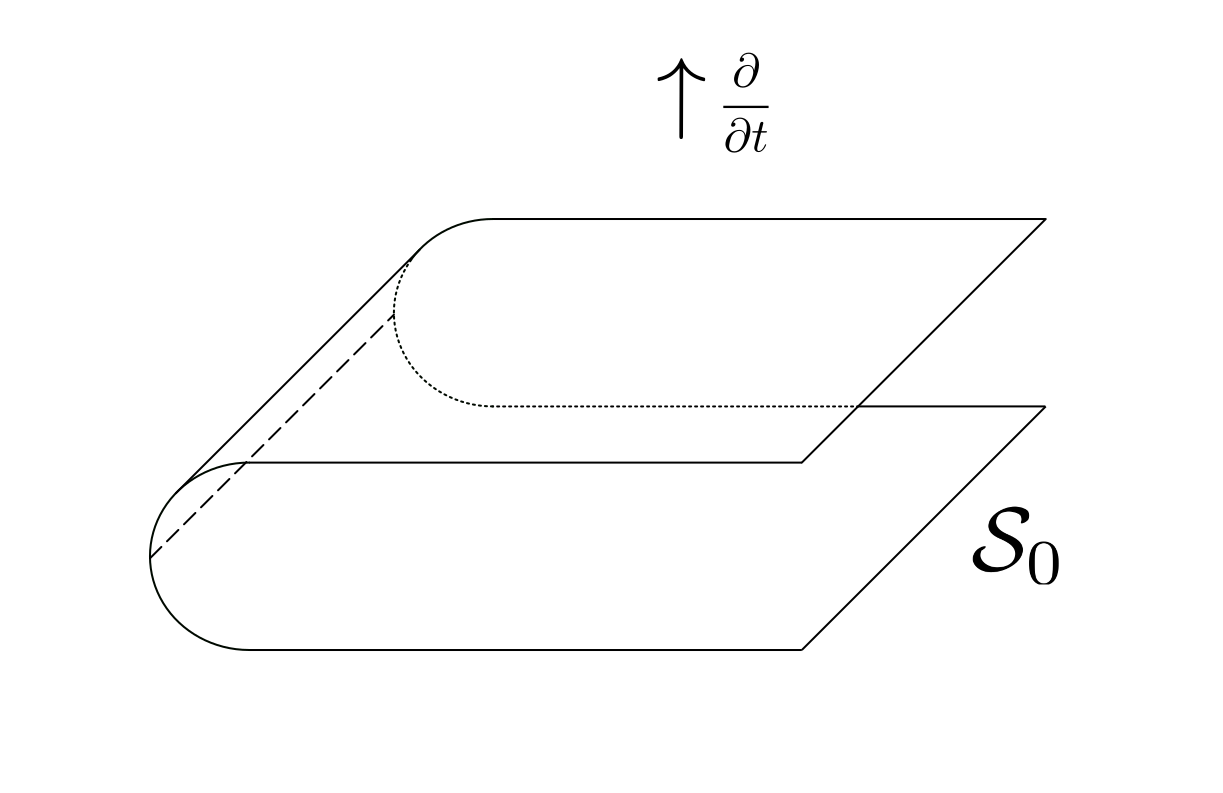
Figure 2: The sketch shows a hypersurface $\mathcal{S}_{0}$ in $(2+1)$-dimensional Minkowski spacetime. At the longly dashed line $\mathcal{S}_{0}$ is tangent to $\partial/\partial t$, so $\partial/\partial t$ cannot be used to define an orientation on $\mathcal{S}_{0}$. In fact, as any Euclidean product of any future-directed causal vector field $J_{0}$ with the respective Euclidean normal vector field on $\mathcal{S}_{0}$ has to change sign and this is continuous by assumption, the non-tangency condition cannot be satisfied on $\mathcal{S}_{0}$—independent of the particular choice of $J_{0}$.

Remark 2.1

We shall consider the particular case that $\left(\mathcal{S}_{0},\iota_{0}\right)$ is spacelike and orientable.

In that instance the metric $g$ on $\mathcal{Q}$ induces a Riemannian metric $\tilde{g}=-\iota_{0}^{*}g$ on $\mathcal{S}_{0}$, which in turn gives rise to a volume form $\tilde{\mu}$ on $\mathcal{S}_{0}$. Denoting the unique future-directed timelike normal vector field over $\mathcal{S}_{0}$ by $\tilde{n}$, we may rewrite the integrand in Eq. (2.2) to

$$\frac{1}{c}\,g_{\iota_{0}(\,.\,)}(J_{0},\tilde{n})\,\,\tilde{\mu}\,.$$ (2.3)

This is indeed the integrand commonly found in the literature.

The integrands in Eqs. (2.2) and (2.3) are, however, not equivalent: If one drops the condition that $(\mathcal{S}_{0},\iota_{0})$ is spacelike, then there may exist points $q$ in $\mathcal{S}_{0}$ for which $(\iota_{0})_{*}\operatorname{T}\negthinspace{}_{q}\mathcal{S}_{0}$ is a lightlike or even timelike subspace of $\operatorname{T}\negthinspace{}_{\iota(q)}\mathcal{Q}$. In the former case the pullback metric is degenerate at $q$ and thus does not give give rise to a volume form. In the latter case there are two normal vectors $\tilde{n}_{q}$, both of them spacelike.

Indeed, there are a number of conceptual problems resulting out of the requirement that $\left(\mathcal{S}_{0},\iota_{0}\right)$ must be spacelike:

1. First, it implicitly and fallaciously associates spacelike hypersurfaces in relativity theory with the Newtonian conception of space. This is problematic, because in non-relativistic physics $c$ is effectively infinite and thus the distinction between lightlike and spacelike hypersurfaces becomes meaningless therein. In a prior work, the first author of this work has argued that ‘Newtonian space’ is more appropriately associated with the past lightcone of the (pointlike) physical observer at an event. We refer to Sec. 3 in Ref. [159].

2. The second problem is one of existence and also concerns the assumption of global hyperbolicity on the spacetime (cf. Sec. 1.4):

   In 1965 Penrose [154] discovered the following property of plane-wave spacetimes:

   No spacelike hypersurface exists in the space-time which is adequate for the global specification of Cauchy data.

   We also refer to Ref. [155] and Chap. 13 in Ref. [10] for a discussion.

   While the argument that such spacetimes are strong idealizations of actual gravitational radiation does have merit, it nonetheless constitutes a weak, physical argument for restricting oneself to spacelike hypersurfaces in globally hyperbolic spacetimes. For the purposes of formulating a quantum theory on curved spacetime, what is the physical argument that in plane-wave spacetimes there should not be any hypersurface ”which is adequate for the global specification of Cauchy data” [154]?

   It seems difficult to justify the two aforementioned assumptions, given that the mathematical theory outlined here exposes them as overly restrictive.

3. The third problem is that in general spacelike hypersurfaces need not stay spacelike under the flow of a time-like/causal/lightlike vector field. We refer to Ex. 3.1 below.

The misconception explained in point 1 above seems to be the main reason why the relativistic $1$-body Born rule had not been stated in its full generality in the literature before. In this respect, it is worth pointing out that Ehlers did not require the non-tangency condition when suggesting the integrand (2.2), though he might have merely omitted it (cf. p. 25 sq. and p. 50 sq. in Ref. [54]). $\diamondsuit$

Having gathered the main ingredients for the $1$-body Born rule in the static case, we are ready to formulate the central theorem of this section.

Theorem 2.1

Let $$\left(\mathcal{Q},g,\mathcal{O}\right) \left(\mathcal{S}_{0},\iota_{0}\right) \mathcal{Q} J_{0} \mathcal{S}_{0}$$ be a spacetime. Further, let be a hypersurface in and let be a nowhere tangent, future-directed timelike/causal/lightlike vector field over .

The following holds:

1. $\mathcal{S}_{0}$ is orientable and carries a canonical orientation.

2. The expression in Eq. (2.2) is a volume form on $\mathcal{S}_{0}$.

3. Let $J_{0}$ satisfy

   $$\frac{1}{c}\int_{\mathcal{S}_{0}}\iota_{0}^{*}\bigl{(}J_{0}\cdot\mu_{\iota_{0}(\,.\,)}\bigr{)}=1\,,$$ (2.4a)

   and denote by $\mathcal{B}^{*}\negthinspace\left(\iota_{0}(\mathcal{S}_{0})\right)$ the $\sigma$-algebra of Lebesgue subsets of the image $\iota_{0}(\mathcal{S}_{0})$. Then

   $$\mathbb{P}_{0}\colon\mathcal{B}^{*}\negthinspace\left(\iota_{0}(\mathcal{S}_{0})\right)\to[0,1]\colon U\mapsto\mathbb{P}_{0}(U)=\frac{1}{c}\int_{\iota_{0}^{-1}(U)}\iota_{0}^{*}\bigl{(}J_{0}\cdot\mu_{\iota_{0}(\,.\,)}\bigr{)}$$ (2.4b)

   defines a probability measure on the measurable space $\bigl{(}\iota_{0}(\mathcal{S}_{0}),\mathcal{B}^{*}\negthinspace\left(\iota_{0}(\mathcal{S}_{0})\right)\bigr{)}$. Moreover, for $U\in\mathcal{B}^{*}\negthinspace\left(\iota_{0}(\mathcal{S}_{0})\right)$ the probability $\mathbb{P}_{0}(U)$ is $0$ if and only if $U$ is a Lebesgue null set.

$\diamondsuit$

The first statement in point 3 of Thm. 2.1 states that $\mathbb{P}_{0}(U)$ is indeed a probability in the mathematical sense of the word. Accordingly, for the static case the (general-relativistic) $1$-body Born rule states that $\mathbb{P}_{0}(U)$ is the probability that the body is located in $U$. Points 1, 2, and the second statement in point 3 are primarily of technical importance.

It is worth pointing out that there is no time given in the prescription $\mathbb{P}_{0}(U)$. The reason is that ‘the time’ is implicit in the choice of $\mathcal{S}_{0}$—which, in accordance with the general principle of relativity, is largely arbitrary.

Formally, we still need to prove that Thm. 2.1 relies on mathematically sensible assumptions.

Proposition 2.1

Let $\left(\mathcal{Q},g,\mathcal{O}\right)$ be a spacetime.

1. There exists an orientable hypersurface $\left(\mathcal{S}_{0},\iota_{0}\right)$ and a future-directed timelike/causal/lightlike vector field $J_{0}$ over $\mathcal{S}_{0}$ such that $J_{0}$ is nowhere tangent to $\mathcal{S}_{0}$.

2. If $J$ is a future-directed timelike/causal/lightlike vector field on $\mathcal{Q}$, then there exists an orientable hypersurface $\left(\mathcal{S}_{0},\iota_{0}\right)$ such that $J_{0}=J_{\iota_{0}(\,.\,)}$ is nowhere tangent to $\left(\mathcal{S}_{0},\iota_{0}\right)$.

$\diamondsuit$

In general, for a given orientable hypersurface $\left(\mathcal{S}_{0},\iota_{0}\right)$ in $\mathcal{Q}$, there need not exist any nowhere-tangent causal vector field over $\mathcal{S}_{0}$. Fig. 2 again provides an example.

For the reader’s convenience we give some coordinate expressions.

Lemma 2.1

Consider the situation of Thm. 2.1 with $$\dim\mathcal{Q}=n+1 n\in\mathbb{N}$$ for .

1. Let $\left(U,\kappa\right)$ be an oriented slice chart for $\mathcal{S}_{0}$ in $\mathcal{Q}$. Denote by $\vec{\kappa}\mapsto\left(0,\vec{\kappa}\right)$ the respective local coordinate expression of $\iota_{0}$. Then for all $W\in\mathcal{B}^{*}\left(\iota_{0}(\mathcal{S}_{0})\cap U\right)$ we have

   $$\mathbb{P}_{0}\left(W\right)=\frac{1}{c}\int_{\vec{\kappa}\left(W\right)}J_{0}^{0}\left(\vec{\kappa}\right)\,\sqrt{-\det{g}}\bigl{(}0,\vec{\kappa}\bigr{)}\,\mathrm{d}^{n}\kappa\,.$$ (2.5a)

2. Let $\left(V,\xi\right)$ and $\left(U,\kappa\right)$ be oriented charts on $\mathcal{S}_{0}$ and $\mathcal{Q}$, respectively, such that $\iota_{0}(V)\cap U$ is nonempty. Denote by $\xi\mapsto\kappa\left(\xi\right)$ the respective local coordinate expression of $\iota_{0}$. Then for all $W\in\mathcal{B}^{*}\bigl{(}\iota_{0}(V)\cap U\bigr{)}$ we have

   $$\mathbb{P}_{0}\left(W\right)=\frac{1}{c}\int_{\xi\left(\iota_{0}^{-1}(W)\right)}(n+1)!\,J_{0}^{[0}(\xi)\,\frac{\partial\kappa^{1}}{\partial\xi^{1}}(\xi)\,\cdots\,\frac{\partial\kappa^{n]}}{\partial\xi^{n}}(\xi)\,\sqrt{-\det{g}}\bigl{(}\kappa\left(\xi\right)\bigr{)}\,\mathrm{d}^{n}\xi\,.$$ (2.5b)

$\diamondsuit$

The following example is meant to illustrate how the relativistic Born rule is to be used in practice and that it is indeed of relevance to relativistic quantum theory.

Example 2.1

Consider Minkowski $$4 \left(\mathbb{R}^{4},g,\mathcal{O}\right) x=\left(ct,\vec{x}\right) \mathcal{O} \partial_{0}=\partial/\partial(ct)$$-spacetime with standard coordinates . As noted above, one may indirectly define the spacetime orientation by declaring that the standard coordinates are oriented and that the timelike vector field is future-directed.

For $i\in\{0,1,2,3\}$ denote by $\gamma^{i}$ the $i$th ‘gamma matrix’. Let $\Psi$ be a section of the trivial bundle $\mathbb{R}^{4}\times\mathbb{C}^{4}$. We think of $\Psi$ as a (smooth) solution of the Dirac equation, possibly in the presence of an external electromagnetic field. We refer, for instance, to Ref. [90] or Sec. 12.2 in Ref. [92].

As indicated in Sec. 1.1, there is some discussion in the physics literature on the interpretation of such ‘Dirac spinor fields’ $\Psi$ and whether the Dirac equation is an acceptable $1$-body evolution equation or not (see e.g. p. 1 and Chap. 1 in Ref. [190]). While this question is ultimately a physical one, Holland [90] has made a convincing argument why (sufficiently regular) Dirac spinor fields do indeed give rise to a mathematically acceptable $1$-body description:

The first point is that the Dirac current $J$ with components

$$J^{i}=\Psi^{\dagger}\cdot\gamma^{0}\cdot\gamma^{i}\cdot\Psi$$ (2.6a)

yields a future-directed timelike vector $J_{x}$ at any $x\in\mathbb{R}^{4}$ for which $\Psi(x)\neq 0$. Thus, if we define the open set

$$\mathcal{Q}=\mathbb{R}^{4}\setminus\Psi^{-1}\left(\{0\}\right)$$ (2.6b)

and restrict $g$, $\mathcal{O}$, $\Psi$, and $J$ accordingly, then $J$ becomes a future-directed timelike vector field on the spacetime $\mathcal{Q}$.

The second such point that speaks for the Dirac theory is that $J$ satisfies the relativistic $1$-body continuity equation and that thus the total probability of finding the body is indeed conserved. A more detailed discussion of this point may be found in Sec. 3.3 below; the particular result is given in Cor. 3.1.4.

These two points make it mathematically possible and sensible to discuss the relativistic $1$-body Born rule within the Dirac theory. In order to keep the discussion here simple, we shall assume, as above, that $\Psi$ and hence $J$ do not vanish. Still, Eq. (2.6i) below holds true regardless.

Having determined $J$ from such a solution $\Psi$ of the Dirac equation, one needs to assure that $J$ is normalized—as one normalizes wave functions in QM. In practice, this is done on the given initial hypersurface $(\mathcal{S}_{0},\iota_{0})$ and then probability conservation guarantees normalization for all other ‘times’. Entirely out of convenience we use

$$\frac{1}{c}\int_{\mathbb{R}^{3}}J^{0}(0,\vec{x})\,\mathrm{d}^{3}x=1$$ (2.6c)

(cf. Lem. 2.1.1).

Assume now that a (pointlike) physical observer is positioned at $x_{0}=(ct_{0},\vec{x}_{0})\in\mathbb{R}^{4}$ and is able to detect the particle in its past light cone $\mathcal{S}_{0}$. Physically, such a detection can only be realized by the interaction of the particle with other matter or radiation, but for the sake of explaining the mathematical theory we shall ignore this complication (see also Footnote 13 above).

Accordingly, we consider the hypersurface

$$\mathcal{S}_{0}=\left\{(ct,\vec{x})\in\mathbb{R}^{4}\middle|t=t_{0}-\left\lvert\vec{x}-\vec{x}_{0}\right\rvert/c<t_{0}\right\}$$ (2.6d)

together with the natural inclusion $\iota_{0}$. It may be shown that the coordinate functions $\vec{x}$ can be restricted to yield coordinates on $\mathcal{S}_{0}$, so that with respect to these coordinates we have

$$\iota_{0}\left(\vec{x}\right)=\left(ct_{0}-\left\lvert\vec{x}-\vec{x}_{0}\right\rvert,\vec{x}\right)=(x^{0}(\vec{x}),\vec{x})$$ (2.6e)

for all $\vec{x}\in\mathbb{R}^{3}\setminus\{0\}$.

As we are only interested in the values of $J$ over $\mathcal{S}_{0}$, the quantity $J$ in the integral in Eq. (2.5b) will be replaced by $J_{0}=J\circ\iota_{0}$. The coordinate representation of the latter is given by

$$J_{0}\colon\vec{x}\mapsto(J_{0})_{\vec{x}}=\left(J^{0}_{0}(\vec{x}),\vec{J}_{0}(\vec{x})\right)=\left(J^{0}\left(\iota_{0}(\vec{x})\right),\vec{J}\left(\iota_{0}(\vec{x})\right)\right)\,.$$ (2.6f)

To compute the respective integrand, we observe that

$$(3+1)!\,J^{[0}(\iota_{0}(\vec{x}))\,\frac{\partial x^{1}}{\partial x^{1}}(\vec{x})\,\frac{\partial x^{2}}{\partial x^{2}}(\vec{x})\,\frac{\partial x^{3]}}{\partial x^{3}}(\vec{x})\\ =\det\begin{pmatrix}J^{0}\left(\iota_{0}(\vec{x})\right)&-\left(\vec{x}-\vec{x}_{0}\right)^{\operatorname{T}}/\left\lvert\vec{x}-\vec{x}_{0}\right\rvert\\ \vec{J}\left(\iota_{0}(\vec{x})\right)&\mathbbm{1}\end{pmatrix}\,.$$ (2.6g)

For a Lebesgue set $U^{\prime}\subseteq\mathbb{R}^{3}$ the probability that the body is in the region

$$U=\iota_{0}\left(U^{\prime}\right)=\left\{\left(ct,\vec{x}\right)\in\mathbb{R}^{4}\middle|t=t_{0}-\left\lvert\vec{x}-\vec{x}_{0}\right\rvert/c<t_{0}\,\,\text{and}\,\,\vec{x}\in U^{\prime}\right\}$$ (2.6h)

of the past light cone of the observer at $x_{0}$ is therefore

$$\mathbb{P}_{0}\left(U\right)=\frac{1}{c}\int_{U^{\prime}}\left(J^{0}\left(\iota_{0}(\vec{x})\right)+\frac{\vec{J}\left(\iota_{0}(\vec{x})\right)\cdot\left(\vec{x}-\vec{x}_{0}\right)}{\left\lvert\vec{x}-\vec{x}_{0}\right\rvert}\right)\,\mathrm{d}^{3}x\,.$$ (2.6i)

In practice it may, however, be simpler to use Cor. 3.1.5 below to compute the respective probability. $\diamondsuit$

We conclude the discussion of the static case with a few remarks.

Remark 2.2

1. Physical arguments have to be employed to show that the integrand in Eq. (2.2) is indeed the physically correct choice.

   Identity (3.18c), which is discussed in Sec. 3.3, may be used as an argument for the ‘naturalness’ of this choice. The identity states that the integrand does not change along the direction of the flow of probability whenever the relativistic continuity equation, $\operatorname{div}J=0$, is satisfied.

   Regardless, a necessary criterion for physical consistency is that the Newtonian limit of the relativistic theory yields the non-relativistic theory: In this limit the non-relativistic $1$-body Born rule must be reobtained, and the demand for probability conservation in the relativistic theory has to carry over to the non-relativistic one. Since the question of the rigorous Newtonian limit is beyond the scope of this article, we shall not discuss this question here. We refer to Sec. 4.2 in Ref. [159] for a rigorous approach.

2. The non-tangency condition alone is in general not sufficient to exclude all hypersurfaces one would want to exclude physically.

   For instance, in Ex. 2.1 the hypersurface

   $$\mathcal{S}_{1}=\left\{(ct,\vec{x})\in\mathbb{R}^{4}\middle|t=0\,\,\text{or}\,\,t=t_{1}\right\}$$ (2.7)

   with $t_{1}\neq 0$ is clearly an unphysical choice, yet so far we have not provided any mathematical condition to exclude it.

   We will provide such a condition in Rem. 3.4 below, noting here only that it is somewhat artificial to consider the Born rule in the absence of any temporal evolution, and that the justification for doing so is primarily pedagogical. We refer to Lem. 3.3 below for an elaboration on how the kinematic Born rule relates to the static one.

   A related point is that one should also require $\left(\mathcal{S}_{0},\iota_{0}\right)$ to be ‘maximal’, so that one normalizes $J$ over ‘the entire space’. Under the additional assumption that $\mathcal{S}_{0}$ is connected, one may define $\left(\mathcal{S}_{0},\iota_{0}\right)$ to be maximal, if there does not exist another connected hypersurface $\left(\mathcal{S}^{\prime}_{0},\iota^{\prime}_{0}\right)$ such that $\iota_{0}(\mathcal{S}_{0})$ is properly contained in $\iota^{\prime}_{0}(\mathcal{S}^{\prime}_{0})$. Usually, however, an appropriate choice of ‘initial hypersurface’ is clear from as well as dictated by physical considerations. In that case, a rigorous mathematical definition would be more cumbersome than useful.

3. For the purpose of measurement one may want to impose more restrictions on the initial hypersurface $\left(\mathcal{S}_{0},\iota_{0}\right)$: For instance, if $J$ is known to be future-directed timelike (which ought to be the case for particles with non-zero mass), yet the values of $J$ are a priori unknown, then the non-tangency condition can only be guaranteed by requiring $\mathcal{S}_{0}$ to be nowhere timelike. This point does, however, not invalidate Rem. 2.1 above.

4. In the related literature some authors consider the Borel $\sigma$-algebra instead of the Lebesgue $\sigma$-algebra for formulating the Born rule on an appropriate manifold $\mathcal{S}_{0}$. The problem with this choice is that it does not yield a complete measure space, which is in turn required to sensibly define $L^{p}$-spaces on $\mathcal{S}_{0}$. $L^{p}$-spaces are important for the mathematical analysis of potential candidates for dynamical equations and, if sensible, for defining spaces of ‘wave functions’. phantom

$\diamondsuit$

3 The kinematic 1-body Born rule

The kinematic Born rule generalizes the static one so as to allow for the temporal evolution of the initial hypersurface. The discussion in Sec. 3.1 below is intended to be a heuristic introduction to the core ideas and, with the exceptions of Prop. 3.1 and Ex. 3.1 below, is therefore not rigorous. The respective mathematical theory will be developed in Secs. 3.2 and 3.3.

3.1 Conceptual approach

We begin by treating the question of how one would generally define the ‘time evolution’ of a hypersurface $(\mathcal{S}_{0},\iota_{0})$ in a spacetime $\mathcal{Q}$.

The reader may recall that in relativity theory the temporal evolution of a single point representing a point mass is generally modeled via a future-directed timelike curve—which is an observer curve in the particular case of proper time parametrization. Moreover, in the geometric optics approximation the propagation of electromagnetic radiation is usually modeled by (a family of) future-directed lightlike curves (cf. Sec. 3.2 in Ref. [174]). Thus, for the purpose of modeling the time evolution of a single point in a spacetime $\mathcal{Q}$ we should consider curves that are future-directed timelike, future-directed lightlike, and perhaps even future-directed causal.

If we view the hypersurface as a collection of points, we may therefore model its evolution by asking that for each $q$ in $\mathcal{S}_{0}$ we have a real open interval $\mathcal{I}_{q}$ and a map $\iota$ such that

$$\iota(\,.\,,q)\colon\mathcal{I}_{q}\to\mathcal{Q}\colon\tau\mapsto\iota(\tau,q)$$ (3.1)

is a future-directed timelike, causal, or lightlike curve.

Moreover, we ask that the tuple $\bigr{(}\mathcal{S}_{0},\iota(\tau,\,.\,)\bigl{)}$ is a hypersurface in its own right and that the curves do not intersect each other for different values of $\tau$. We also do not allow tearing, since, heuristically speaking, at the given ‘parameter time’ $\tau$ this would make $\iota$ discontinuous in $q$. Leaving the precise mathematical construction for Sec. 3.2 below, we find that the domain $\mathcal{S}$ of $\iota$ ought to be an open subset of $\mathbb{R}\times\mathcal{S}_{0}$, obtained by taking the disjoint union of all the intervals $\mathcal{I}_{q}$, and that $\iota$ itself ought to be a diffeomorphism to its image (or at least a local diffeomorphism; see Rem. 3.1.2 below).

Borrowing terminology from the non-relativistic continuum mechanics, this is indeed the general idea of how the temporal evolution is modeled in the Lagrangian picture. As in the non-relativistic analogue, the map $\iota$ fixes the initial point $q$ and then follows its trajectory as $\tau$ increases.

In the non-relativistic theory, one may, however, take another point of view known as the Eulerian picture. In the relativistic theory this is also a valid approach: Here the evolution of the hypersurface $(\mathcal{S}_{0},\iota_{0})$ is indirectly determined by a future-directed timelike, lightlike, or even causal vector field $X$ on $\mathcal{Q}$. The velocity vector field $X$ then gives rise to a flow $\Phi$, which in turn connects the Eulerian picture with the Lagrangian picture via the relation

$$\iota(\tau,q)=\Phi_{\tau}\bigl{(}\iota_{0}(q)\bigr{)}\,.$$ (3.2)

A schematic illustration of how the time evolution of a hypersurface may be modeled in the relativistic theory is given in Fig. 3.

Figure 3: The sketch illustrates the general idea of how to define the time evolution of an initial hypersurface $\mathcal{S}_{0}$, here given as a subset of a spacetime $\mathcal{Q}$: In the Lagrangian picture, one evolves every point in $\mathcal{S}_{0}$ along a future-directed timelike, causal, or lightlike curve, as given by Eq. (3.1). Each ‘parameter time’ $\tau$ then gives rise to a new hypersurface, namely the image $\iota(\tau,\mathcal{S}_{0})$. In the Eulerian picture, on the other hand, one considers the velocity field $X$ instead, which is a future-directed timelike, causal, or lightlike vector field on $\mathcal{Q}$ that is nowhere tangent to $\mathcal{S}_{0}$. The flow of $X$ relates the two pictures.

Of course, the described approach is of little use, if it cannot be shown to be consistent with the static Born rule of Sec. 2. To make the two consistent, two points require elaboration: First, what is the relation between the vector fields $J$ and $X$? Second, does the suggested time evolution model respect the non-tangency condition of the hypersurface? After all and in accord with the general principle of relativity, the underlying theory should be independent of which hypersurface one chooses as initial.

Regarding the first point, recall that in the static case we assumed that the dynamics of the respective $1$-body quantum theory provides us with a future-directed timelike, causal, or lightlike current density vector field $J$ on $\mathcal{Q}$. It would therefore be mathematically sensible to set the two vector fields $J$ and $X$ equal.

Yet this choice is physically incorrect, because the components of $J$ and $X$ have different physical dimensions: This can be seen by considering, for instance, the components $J^{i}$ of $J$ and $X^{i}$ of $X$, respectively, in standard coordinates in Minkowski spacetime. By assumption, each $J^{i}$ has the physical dimension of a probability current—velocity times inverse volume. The components $X^{i}$, on the other hand, appear in the integral curve equation, and thus have the physical dimension of velocity.

Nonetheless, we do interpret the ‘direction’ of $J$ as the ‘propagation direction’ of probability. Therefore, we require that there exists a strictly positive – though usually not constant – factor of proportionality $\rho$:

$$J=\rho\,X\,.$$ (3.3)

Eq. (3.3) is the relativistic analogue of the respective non-relativistic relation between a current density vector field on the one hand and the probability density and (drift) velocity vector field on the other—i.e. $\vec{j}=\rho\,\vec{v}$.

This, of course, raises the question of how to determine $\rho$ from $J$. In the analogue theories in which $J$ is a mass or a charge current density (cf. Rem. 1.1), $J$ will be timelike and $\rho$ may then be obtained by requiring that the integral curves of $X$ are observer curves. That is, $X$ is future-directed and satisfies

$$g(X,X)=c^{2}\,.$$ (3.4)

In quantum theory, however, Eq. (3.4) is more difficult to justify. The $1$-body Dirac theory discussed in Ex. 2.1, for instance, is agnostic with regards to the question.

In the absence of any other physical conditions, using Eq. (3.4) to determine $X$ from $J$ via Eq. (3.3) is arguably a natural choice. Ultimately, the theory we lay out in this work does not depend on this choice, however, with different choices amounting to a mere redefinition of the respective quantities (cf. Rem. 3.6 below). In practical applications one may therefore make a choice that is computationally convenient.

However one chooses the factor $\rho$, it will have the physical dimension of a probability density and, if one wants to bestow independent physical significance upon it, the choice should be independent of a particular coordinate system, again in accordance with the general principle of relativity. The first person to suggest the definition of such an invariant quantity was Eckart, who in the context of special-relativistic fluid mechanics introduced an invariant (inertial) mass density $\rho$ satisfying Eq. (3.3) for a mass current density $J$ by requiring $X$ to fulfill Eq. (3.4). Inspired by his work, in the context of relativistic quantum theory we suggest to call $\rho$ an invariant probability density, provided that the condition to obtain it from the probability current density $J$ is coordinate-invariant as well—as it is the case for Eq. (3.4).

A physical advantage of introducing an invariant probability density $\rho$ in this manner is that it allows one to conceptually separate the vector field governing the evolution of the hypersurface – namely $X$ – from the ‘amount of probability’ contained in each one of its ‘regions’ at different ‘times’—the scalar field $\rho$. Indeed, we will see below that, while the Eulerian picture alone in principle only needs the vector field $J$ for its full formulation, the Lagrangian picture indirectly relies on Eq. (3.3) (via the map $\iota$).

The second question above has a more straightforward answer: The following proposition shows that the evolution does indeed respect the non-tangency condition.

Proposition 3.1

Let $\mathcal{Q}$ be a manifold and let $X$ be a vector field on $\mathcal{Q}$ that is nowhere tangent to a an embedded submanifold $(\mathcal{S}_{0},\iota_{0})$ in $\mathcal{Q}$. Further, let $\Phi$ be the flow of $X$ and let $\tau$ be any real number such that the image $\mathcal{S}_{\tau}=\Phi_{\tau}\bigl{(}\iota_{0}(\mathcal{S}_{0})\bigr{)}$ is defined.

Then $\mathcal{S}_{\tau}$ is an embedded submanifold of $\mathcal{Q}$ that is nowhere tangent to $X$. $\diamondsuit$

On the contrary, the following example shows that an initially spacelike hypersurface need not remain spacelike under the flow of a future-directed timelike vector field—even in the absence of curvature (cf. Rem. 2.1 above).

Example 3.1

In Minkowski $$3 (ct,x,y) \omega>0 X$$-spacetime, standard coordinates thereon, and for some consider the observer (vector) field with values

$$\vec{X}(ct,x,y) =\omega\,\begin{pmatrix}0&-1\\ 1&0\end{pmatrix}\cdot\begin{pmatrix}x\\ y\end{pmatrix}\,,$$ (3.5a)

$$X^{0}(ct,x,y) =c\sqrt{1+\left(\vec{X}(t,x,y)/c\right)^{2}}\,.$$ (3.5b)

Physically, this vector field describes a rotation about the observer curve $$\tau\mapsto(c\tau,0,0) \mathbb{R}^{3} 2$$ in . As Eq. (3.5a) is the equation of a linear vector field (cf. §1.1 in [79] and Ex. 3.2.8 in [167]) and the respective matrix factor is in the Lie algebra of the -dimensional rotation group, we find by exponentiation that

$$\Phi_{\tau}(t_{0},x_{0},y_{0})=\begin{pmatrix}\sqrt{c^{2}+\omega^{2}(x_{0}^{2}+y_{0}^{2})}\,\tau+ct_{0}\\ x_{0}\,\cos(\omega\tau)-y_{0}\,\sin(\omega\tau)\\ x_{0}\sin(\omega\tau)+y_{0}\cos(\omega\tau)\end{pmatrix}\,.$$ (3.5c)

Consider now the initial hypersurface $\mathcal{S}_{0}=\mathbb{R}^{2}$ with

$$\iota_{0}\colon\mathcal{S}_{0}\to\mathbb{R}^{3}\colon(x_{0},y_{0})\mapsto\iota_{0}(x_{0},y_{0})=(0,x_{0},y_{0})\,.$$ (3.5d)

Upon setting $r_{0}:=\sqrt{x_{0}^{2}+y_{0}^{2}}$, the unit radial tangent vector at $(x_{0},y_{0})\neq(0,0)$ that points away from the origin in $\mathcal{S}_{0}$ is given by

$$\hat{r}_{(x_{0},y_{0})}=\left.\frac{\partial}{\partial r}\right\rvert_{(x_{0},y_{0})}=\frac{1}{r_{0}}\,\begin{pmatrix}x_{0}\\ y_{0}\end{pmatrix}\,.$$ (3.5e)

A calculation reveals that the pushforward of $\hat{r}_{(x_{0},y_{0})}$ under the map

$$\iota(\tau,\,.\,)=\Phi_{\tau}\circ\iota_{0}\colon\mathcal{S}_{0}\to\mathbb{R}^{3}\colon(x_{0},y_{0})\mapsto\iota(\tau,x_{0},y_{0})=\Phi_{\tau}(0,x_{0},y_{0})$$ (3.5f)

with $\tau\in\mathbb{R}$ becomes lightlike at proper time

$$\tau=\frac{\sqrt{c^{2}+\omega^{2}r_{0}^{2}}}{\omega^{2}r_{0}}$$ (3.5g)

and stays timelike afterwards. Therefore, the hypersurface $\mathcal{S}_{\tau}=\iota(\tau,\mathcal{S}_{0})$ is spacelike for $\tau=0$ and fails to be spacelike for any $\tau>0$. The qualitative time evolution of $\mathcal{S}_{0}$ is illustrated in Fig. 4. $\diamondsuit$

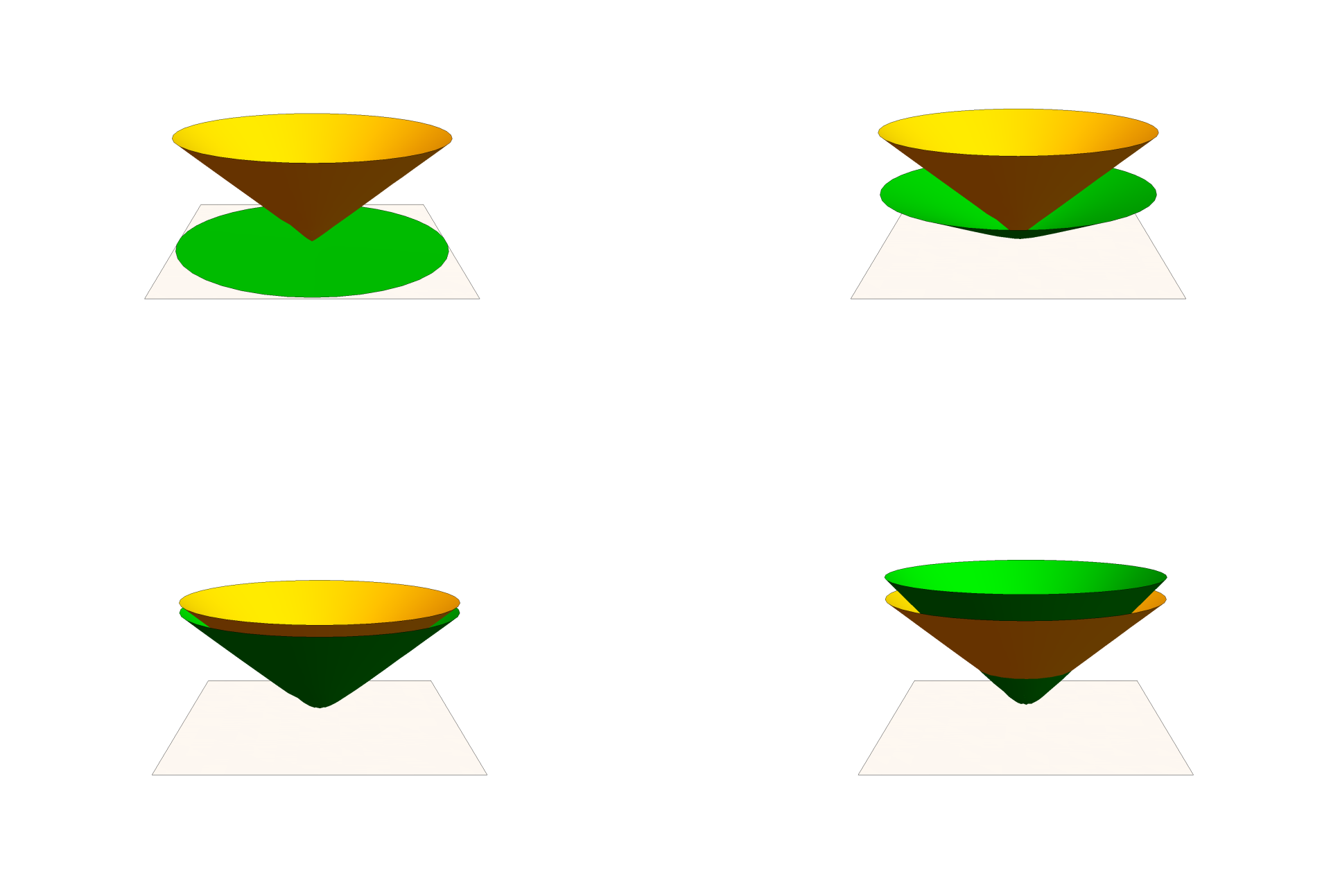
Figure 4: For Ex. 3.1 this figure illustrates the qualitative temporal evolution of a circular, green disk, initially lying in the $(t=0)$-hypersurface $\iota_{0}(\mathcal{S}_{0})$. Subsequent time steps are shown from left to right and from top to bottom. For each time step the white plane represents $\iota_{0}(\mathcal{S}_{0})$. The yellow future light cone of the observer curve $\tau\mapsto(c\tau,0,0)$ moves upwards along the $ct$-axis, its tip always touching the disk. In the first three time steps, the disk bends towards the light cone, but does not intersect it—it stays spacelike. In the last time step, however, the disk has crossed the light cone—its causal character has changed.

The behavior exhibited in Ex. 3.1 seems to be generic. Indeed, we recently gave another example of a flow on a curved spacetime (Ex. 3 in Ref. [162]), that also does not preserve the spacelikeness of the initial hypersurface.

3.2 The Lagrangian picture

Having the central ideas of the Lagrangian picture in place, we proceed with the development of the rigorous theory. First we define a suitable class of domains for the above map $\iota$.

Definition 3.1

A flow domain $\mathcal{S}$ for a manifold $\mathcal{S}_{0}$ is an open subset of the product $\mathbb{R}\times\mathcal{S}_{0}$ such that for every $q$ in $\mathcal{S}_{0}$ the set

$$\mathcal{I}_{q}=\left\{\tau\in\mathbb{R}\middle|\left(\tau,q\right)\in\mathcal{S}\right\}$$ (3.6)

is an open interval (cf. p. 211 in Ref. [119]). $\diamondsuit$

Of course, the domain of any flow of a vector field on $\mathcal{S}_{0}$ will be a flow domain.

Yet for our purposes we are interested in the case that $\left(\mathcal{S}_{0},\iota_{0}\right)$ is an embedded submanifold of a manifold $\mathcal{Q}$ and that $\Phi$ is the (maximal) flow of a vector field $X$. In that instance, a flow domain is obtained by taking the (maximal) domain $\mathcal{S}$ on which the map

$$\iota\colon\mathcal{S}\to\mathcal{Q}\colon(\tau,q)\mapsto\iota(\tau,q)=\Phi_{\tau}\bigl{(}\iota_{0}(q)\bigr{)}$$ (3.7)

is well-defined.

The conceptual advantage of defining flow domains for $\mathcal{S}_{0}$ intrinsically, i.e. independent of any flow on $\mathcal{Q}$, is that, in the case that the above map $\iota$ is not surjective, one can forget about the values of $\Phi$ that do not lie in the image $\iota(\mathcal{S})$. Those points are not of relevance to the temporal evolution of the hypersurface. As noted in Sec. 1.3, this intrinsic approach turns out to be of fundamental importance for the many-body generalization.

Accordingly, in the next step we provide a definition that captures the intrinsic properties of the tuple $\left(\mathcal{S},\iota\right)$. It is at this point that the non-tangency condition appears in the Lagrangian picture.

Definition 3.2

Let $$\mathcal{Q} \left(\mathcal{S}_{0},\iota_{0}\right) \mathcal{Q}$$ be a manifold and let be an embedded submanifold of .

1. A flowout from $\left(\mathcal{S}_{0},\iota_{0}\right)$ is a tuple $\left(\mathcal{S},\iota\right)$ such that

   1. $\mathcal{S}$ is a flow domain for $\mathcal{S}_{0}$,

   2. the map

      $$\iota\colon\mathcal{S}\to\mathcal{Q}\colon(\tau,q)\mapsto\iota(\tau,q)$$ (3.8a)

      satisfies $\iota_{0}=\iota(0,\,.\,)$, and

   3. $\left(\mathcal{S},\iota\right)$ is an embedded submanifold of $\mathcal{Q}$.

2. If $X$ is a vector field on $\mathcal{Q}$ that is nowhere tangent to $\left(\mathcal{S}_{0},\iota_{0}\right)$, then the tuple $\left(\mathcal{S},\iota\right)$ is called a flowout from $\left(\mathcal{S}_{0},\iota_{0}\right)$ along $X$, if $\left(\mathcal{S},\iota\right)$ is a flowout from $\left(\mathcal{S}_{0},\iota_{0}\right)$ and we have

   $$X_{\iota(\tau,q)}=\iota_{*}\,\left.\frac{\partial}{\partial\tau}\right\rvert_{(\tau,q)}$$ (3.8b)

   for all $(\tau,q)\in\mathcal{S}$.

   The respective flowout is maximal, if there does not exist another flowout $\left(\mathcal{S}^{\prime},\iota^{\prime}\right)$ from $\left(\mathcal{S}_{0},\iota_{0}\right)$ along $X$ such that $\mathcal{S}\subset\mathcal{S}^{\prime}$.

$\diamondsuit$

It is a simple consequence of the above definition that the vector field $\iota_{*}(\partial/\partial\tau)$ is nowhere tangent to $\bigl{(}\{\tau\}\times\mathcal{S}_{0},\iota(\tau,\,.\,)\bigr{)}$ for all $\tau\in\mathbb{R}$ such that $\operatorname{dom}\iota(\tau,\,.\,)=\mathcal{S}_{0}$. As shown in the proof of Thm. 2.1.1, this means that a hypersurface $\left(\mathcal{S}_{0},\iota_{0}\right)$ in $\mathcal{Q}$ can only admit a flowout, if it is orientable.

Remark 3.1

Three points are worthy of note with regards to Def. 3.2:

1. In Ref. [119] Lee does not require flowouts $\left(\mathcal{S},\iota\right)$ to be embedded.

   His flowout theorem states the following (Thm. 9.20 in Ref. [119]): Given a vector field $X$ on a manifold $\mathcal{Q}$ that is nowhere tangent to an embedded submanifold $\left(\mathcal{S}_{0},\iota_{0}\right)$ of $\mathcal{Q}$ and has flow $\Phi$, it is always possible to find a (not necessarily maximal) flow domain $\mathcal{S}$ for $\mathcal{S}_{0}$ such that the map $\iota$ in Eq. (3.7) is an injective immersion. That is, $\left(\mathcal{S},\iota\right)$ is only an ‘immersed’ submanifold, not an embedded one.

   While $\iota$ is indeed a smooth embedding whenever $\left(\mathcal{S}_{0},\iota_{0}\right)$ is a hypersurface (point (d) in the above theorem), we conjecture that the general result may be strengthened in this manner regardless of dimension. To our knowledge, however, no such theorem exists in the literature. Despite this, Def. 3.2 does implicitly rely on this more general statement.

2. There do indeed exist ‘non-embedded flowouts’. An example of such a ‘non-embedded flowout’ from a $0$-dimensional submanifold is given in Ex. 4.20 of Ref. [119]. In that instance the image $\iota(\mathcal{S})$ is dense in the ambient manifold $\mathcal{Q}$.

   Nonetheless, it does not constitute a counterexample to the conjecture in point 1 above, because an ‘embedded flowout’ may be obtained via a restriction in domain $\mathcal{S}$ of the map $\iota$. The example does show, however, that a maximal ‘embedded flowout’ need not always exist.

3. Def. 3.2 does not adequately account for the case that there exists a periodic integral curve of $X$ that intersects $\left(\mathcal{S}_{0},\iota_{0}\right)$ (which would imply that the spacetime is ‘vicious’, cf. Sec. 4.2 in Ref. [138]):

   If such a curve exists and $\Phi$ is the maximal flow of $X$, then the map $\iota$ in Eq. (3.7) will not be injective on its maximal domain $\mathcal{S}$. While the existence of such timelike/causal loops is often viewed as physically problematic (cf. Ref. [139] and p. 407 in Ref. [145]), Def. 3.2 is of purely mathematical nature and should therefore account for the possibility of periodic integral curves.

   In Appx. Proof below we show how Def. 3.2 ought to be generalized to this case.

   While it would be worthwhile to consider the theory in this article in this more general context, it would also make the mathematical relation between the Lagrangian and the Eulerian picture more subtle. In particular, Lem. 3.1 below would have to be turned into a local statement. We shall therefore abstain from using this more general definition here.

$\diamondsuit$

It should be clear from the discussion in the beginning of this section that for the purposes of relativistic quantum theory we need to further constrain the classes of flowouts. Indeed, doing so constitutes the first major step in the construction of the Lagrangian picture.

Definition 3.3

Let $\left(\mathcal{Q},g,\mathcal{O}\right)$ be a spacetime and let $\left(\mathcal{S}_{0},\iota_{0}\right)$ be an orientable hypersurface in $\mathcal{Q}$.

A future directed timelike 1-body flowout (from $\left(\mathcal{S}_{0},\iota_{0}\right)$) is a flowout $\left(\mathcal{S},\iota\right)$ from $\left(\mathcal{S}_{0},\iota_{0}\right)$ such that

$$\mathcal{X}=\iota_{*}\,\frac{\partial}{\partial\tau}$$ (3.9)

is a future-directed timelike vector field over $\mathcal{S}$.

Analogously, we define future-directed lightlike and future-directed causal $1$-body flowouts by requiring $\mathcal{X}$ to have the respective property. $\diamondsuit$

While it is in principle possible to consider past-directed timelike/causal/lightlike $1$-body flowouts in Def. 3.3 instead, because ‘time flows forward’ this would constitute an unconventional choice. Yet defining ‘spacelike 1-body flowouts’ would be physically inadequate, since a flowout for which $\mathcal{X}$ is spacelike cannot describe any temporal evolution of a $1$-body quantum system.

The following proposition provides a general existence result for $1$-body flowouts.

Proposition 3.2

In any spacetime the following holds:

1. There exists a future-directed timelike/causal/lightlike $1$-body flowout.

2. Given a future-directed timelike/causal/lightlike vector field $X$ on the spacetime and a hypersurface $\left(\mathcal{S}_{0},\iota_{0}\right)$ such that $X$ is nowhere tangent, there exists a future-directed timelike/causal/lightlike $1$-body flowout from $\left(\mathcal{S}_{0},\iota_{0}\right)$ along $X$.

3. If $X_{0}$ is a nowhere tangent, future-directed timelike vector field over a hypersurface $\left(\mathcal{S}_{0},\iota_{0}\right)$ in the spacetime, then there exists a future-directed timelike vector field $X$ in a neighborhood of $\iota_{0}(\mathcal{S}_{0})$ and a future-directed timelike $1$-body flowout $\left(\mathcal{S},\iota\right)$ from $\left(\mathcal{S}_{0},\iota_{0}\right)$ along $X$ such that for all $q$ in $\mathcal{S}_{0}$ we have

   $$(X_{0})_{q}=X_{\iota_{0}(q)}=X_{\iota(0,q)}\,.$$ (3.10)

$\diamondsuit$

Point 3 of Prop. 3.2 essentially states that it is always possible to extend the construction in Sec. 2 to a kinematic description, at least in the timelike case.

The second major step in the construction of the Lagrangian picture is to show that one may think of the flow domain $\mathcal{S}$ as a spacetime in its own right.

Lemma 3.1

Let $\left(\mathcal{Q},g,\mathcal{O}\right)$ be a spacetime and let $\left(\mathcal{S},\iota\right)$ be a future-directed timelike/causal/lightlike $1$-body flowout. Further, let $\tilde{\iota}$ be the restriction of $\iota$ in codomain to its image in $\mathcal{Q}$.

Then $\left(\mathcal{S},\iota^{*}g,\left(\tilde{\iota}^{-1}\right)_{*}\mathcal{O}\right)$ is a spacetime isomorphic to $\bigl{(}\iota(\mathcal{S}),g\negthickspace\upharpoonright_{\iota(\mathcal{S})},\operatorname{Fr}(\iota(\mathcal{S}))\cap\mathcal{O}\bigr{)}$. $\diamondsuit$

Because of Lem. 3.1, one may ‘forget’ about the spacetime $\mathcal{Q}$ and ‘carry’ the physical description over to $\mathcal{S}$ instead, at least for the purpose of the kinematic Born rule. Indeed, one may freely switch between the two descriptions via the diffeomorphism $\tilde{\iota}$.

It is therefore justified to ask for the probability that the body is in a ‘region’ $U$ in a certain hypersurface in $\mathcal{S}$, as opposed to a ‘region’ in an admissible hypersurface in $\mathcal{Q}$. This is indeed how we will formulate the kinematic $1$-body Born rule in the Lagrangian picture.

Remark 3.2

If $\iota(\mathcal{S})$ is properly contained in $\mathcal{Q}$, then the spacetime $\mathcal{S}$ in Lem. 3.1 may have different causal properties. It is, for instance, not possible for $\mathcal{S}$ to contain causal loops, since that would contradict injectivity of $\iota$. We refer the reader to Rem. 3.1.3 and Appx. Proof. Refs. [139, 138] provide a general discussion of the causal properties of spacetimes. $\diamondsuit$

While the discussion in the introduction of this section and Fig. 3 do explain the central ideas of the kinematic description, they are also potentially misleading: They implicitly suggest that the hypersurfaces $\{\tau\}\times\mathcal{S}_{0}\subset\mathcal{S}$ with $\tau\in\mathbb{R}$ are the only ones of interest in the Lagrangian picture (or, equivalently, their images in $\mathcal{Q}$ under $\iota$). This would, however, indirectly contradict the general principle of relativity. Just as one should be able to freely choose the initial hypersurface $\left(\mathcal{S}_{0},\iota_{0}\right)$ in $\mathcal{Q}$, hypersurfaces of the type $\{\tau\}\times\mathcal{S}_{0}$ ought not to hold any particular physical significance.

In order to mathematically account for this insight, we introduce the concept of a ‘timeshift’.

Definition 3.4

Let $\left(\mathcal{S},\iota\right)$ be a flowout from a submanifold $\left(\mathcal{S}_{0},\iota_{0}\right)$ in a manifold $\mathcal{Q}$.

We call a (smooth) function $\mathcal{T}$ on $\mathcal{S}_{0}$ such that its graph $\operatorname{graph}(\mathcal{T})$ is contained in $\mathcal{S}$ a shift (of $\left(\mathcal{S}_{0},\iota_{0}\right)$ in $\mathcal{S}$). If in addition $\left(\mathcal{S},\iota\right)$ is a future-directed timelike/causal/lightlike $1$-body flowout, then the shift $\mathcal{T}$ is called a timeshift (of $\left(\mathcal{S}_{0},\iota_{0}\right)$ in $\mathcal{S}$). $\diamondsuit$

The general idea of a shift $\mathcal{T}$ is that it induces a mapping

$$\iota_{\mathcal{T}}\colon\mathcal{S}_{0}\to\mathcal{S}\colon q\mapsto\iota_{\mathcal{T}}(q)=\iota\bigl{(}\mathcal{T}(q),q\bigr{)}$$ (3.11)

which ‘shifts’ the submanifold $\left(\mathcal{S}_{0},\iota_{0}\right)$ to the submanifold $\left(\mathcal{S}_{0},\iota_{\mathcal{T}}\right)$ in $\mathcal{Q}$.

Accordingly, in the Lagrangian picture timeshifts model the time evolution of the relativistic $1$-body system: For $\tau\in\mathbb{R}$ the hypersurface $\{\tau\}\times\mathcal{S}_{0}$ in $\mathcal{S}$ is obtained by choosing the particular timeshift $\mathcal{T}$ with values $\mathcal{T}(q)=\tau$ for all $q\in\mathcal{S}_{0}$—but in the general case there is no requirement for $\mathcal{T}$ to be constant. An illustration is given in Fig. 59.

Figure 5: This sketch shows how the Born rule is formulated in the Lagrangian picture. The initial hypersurface is $\mathcal{S}_{0}$, given as the subset $\{0\}\times\mathcal{S}_{0}$ in the depiction. The respective flow domain $\mathcal{S}\subseteq\mathbb{R}\times\mathcal{S}_{0}$ is enclosed by the dashed line and, in this instance, partially unbounded in positive $\tau$-direction. Following Lem. 3.1, the general idea is that the manifold $\mathcal{S}$ allows one to reformulate the dynamics in $\mathcal{Q}$ such that said dynamics becomes trivial (it is implicitly encoded in the map $\iota\colon\mathcal{S}\to\mathcal{Q}$). As in the static case, we formulate the Born rule on (the image of) an embedded hypersurface—yet in the Lagrangian picture this hypersurface is the graph of a timeshift $\mathcal{T}$, shown here in gray. If one has probability conservation, then for a given ‘region’ $U\subseteq\operatorname{graph}(\mathcal{T})$ the probability to find the body in a subset $\iota(U)$ of $\iota(\operatorname{graph}(\mathcal{T}))$ is simply the probability to find the body in the subset $\iota_{0}\left(\operatorname{pr}_{2}(U)\right)$ of $\iota_{0}\left(\mathcal{S}_{0}\right)$ (cf. Thm. 3.1.5).

Having gathered all the main ingredients of the Lagrangian picture, we may now state the respective central theorem.

Theorem 3.1

Let $$\left(\mathcal{Q},g,\mathcal{O}\right) \left(\mathcal{S},\iota\right) 1 \left(\mathcal{S}_{0},\iota_{0}\right) \mathcal{Q}$$ be a spacetime. Let be a future-directed timelike/causal/lightlike -body flowout from a hypersurface in .

Furthermore, let $\mathcal{T}$ be a timeshift of $\mathcal{S}_{0}$ in $\mathcal{S}$ and define the function

$$\mathcal{T}^{\prime}\colon\mathcal{S}_{0}\to\mathcal{S}\colon q\mapsto\mathcal{T}^{\prime}(q)=(\mathcal{T}(q),q)\,.$$ (3.12a)

The following holds:

1. 1. $\bigl{(}\mathcal{S}_{0},\mathcal{T}^{\prime}\bigr{)}$ is an embedded submanifold of $\mathcal{S}$ that is equivalent to $\operatorname{graph}(\mathcal{T})$ (together with its natural inclusion in $\mathcal{S}$), and

   2. $\operatorname{graph}(\mathcal{T})$ is orientable and carries a canonical orientation.

2. Denote by $\mu$ the canonical volume form on $\mathcal{Q}$. Then

   $$\upsilon=\frac{1}{c}\,\frac{\partial}{\partial\tau}\cdot\iota^{*}\mu$$ (3.12b)

   restricts to a volume form on $\operatorname{graph}(\mathcal{T})$. Moreover, $\left(\mathcal{T}^{\prime}\right)^{*}\upsilon$ is a volume form on $\mathcal{S}_{0}$.

3. Choose any (smooth) strictly positive scalar field $\varrho$ on $\mathcal{S}$. Then there exists a unique scalar field $\mathring{\varrho}$ on $\mathcal{S}$ such that

   $$\frac{\partial}{\partial\tau}\left(\varrho\,\upsilon\right)=\mathring{\varrho}\,\upsilon\,.$$ (3.12c)

4. Set $\operatorname{graph}(0)=\{0\}\times\mathcal{S}_{0}\subset\mathcal{S}$. Let $\varrho$ as above satisfy

   $$\int_{\operatorname{graph}(0)}\varrho\,\upsilon=1$$ (3.12d)

   and $\mathring{\varrho}=0$. Then

   $$\mathbb{P}_{\text{L}}\colon\mathcal{B}^{*}\negthinspace\bigl{(}\operatorname{graph}(\mathcal{T})\bigr{)}\to[0,1]\colon U\mapsto\mathbb{P}_{\text{L}}(U)=\int_{U}\varrho\,\upsilon$$ (3.12e)

   defines a probability measure on the measurable space $\bigl{(}\operatorname{graph}(\mathcal{T})$, $\mathcal{B}^{*}\negthinspace(\operatorname{graph}(\mathcal{T}))\bigr{)}$. Moreover, for $U\in\mathcal{B}^{*}\negthinspace\left(\operatorname{graph}(\mathcal{T})\right)$ the probability $\mathbb{P}_{\text{L}}(U)$ is $0$ if and only if $U$ is a Lebesgue null set.

5. Consider the projection mapping

   $$\operatorname{pr}_{2}\colon\mathcal{S}\to\mathcal{S}_{0}\colon(\tau,q)\mapsto\operatorname{pr}_{2}(\tau,q)=q\,.$$ (3.12f)

   If $\varrho$ satisfies the properties of point 4 above, then for all $U\in\mathcal{B}^{*}\negthinspace\left(\operatorname{graph}(\mathcal{T})\right)$ we have

   $$\mathbb{P}_{\text{L}}(U)=\int_{\operatorname{pr}_{2}(U)}\varrho(0,\,.\,)\,\upsilon_{(0,\,.\,)}=\mathbb{P}_{\text{L}}\bigl{(}0^{\prime}(\operatorname{pr}_{2}(U))\bigr{)}\,.$$ (3.12g)

   In particular, $\mathbb{P}_{\text{L}}(U)$ only depends on $\operatorname{pr}_{2}(U)$, which is independent of the choice of $\mathcal{T}$.

$\diamondsuit$

Point 1 of Thm. 3.1 is a consistency result. Point 2 shows that $\upsilon$ may be viewed as a ‘spatial volume form’. Point 3 gives rise to the Langrangian continuity equation, that is the continuity equation in the Lagrangian picture:

$$\mathring{\varrho}=0\,.$$ (3.13)

Moreover, Eq. (3.12c) identifies $\mathring{\varrho}$ as a geometric invariant—which is of particular relevance whenever one lifts the requirement of probability conservation (cf. Sec. 4). Point 4 states that the kinematic $1$-body Born rule in the Langrangian picture, Eq. (3.12e), does indeed yield a probability in the strict mathematical sense – that is probability conservation holds – whenever the Lagrangian continuity equation is satisfied. Regarding the relation of point 4 to the general principle of relativity we refer to Sec. 1.2 and Footnote 25 above. If probability conservation holds, then point 5 provides us with a simple way to compute the respective probability.

Remark 3.3

The reader may have noticed that the notation $\mathbb{P}_{\text{L}}(U)$ for the respective probability does not make any explicit reference to a choice of timeshift. There is indeed a mathematical justification for this notation:

Consider the set

$$\mathcal{B}^{*}_{\text{L}}\negthinspace\left(\mathcal{S}\right)=\left\{U\subset\mathcal{S}\middle|\exists\,\,\text{timeshift}\,\,\mathcal{T}\colon\,\,U\in\mathcal{B}^{*}\negthinspace\bigl{(}\operatorname{graph}(\mathcal{T})\bigr{)}\right\}\,.$$ (3.14)

Since for $U\in\mathcal{B}^{*}\negthinspace\bigl{(}\operatorname{graph}(\mathcal{T})\bigr{)}$ the integral in Eq. (3.12e) does not depend on the values of the timeshift $\mathcal{T}$ on $\operatorname{graph}(\mathcal{T})\setminus U$, we may understand $\mathbb{P}_{\text{L}}$ as a map from $\mathcal{B}^{*}_{\text{L}}\negthinspace\left(\mathcal{S}\right)$ to the interval $[0,1]$. The downside of this approach is that $\mathbb{P}_{\text{L}}$ then ceases to be a probability measure in the mathematical sense, because $\mathcal{B}^{*}_{\text{L}}\negthinspace\left(\mathcal{S}\right)$ does not contain $\mathcal{S}$ itself and is thus not a $\sigma$-algebra.

Indeed, one may pursue this approach further and even define respective ‘Lagrangian $L^{p}$-spaces’ (cf. Rem. 2.2.4). Since we only treat the smooth case here, however, we shall abstain from a more detailed treatment thereof.

Also note that the Lagrangian continuity equation (3.13) does not need to hold for the above definition of $\mathbb{P}_{\text{L}}$ to be sensible. $\diamondsuit$

The next lemma provides local coordinate expressions for $\mathring{\varrho}$ and $\mathbb{P}_{\text{L}}$.

Lemma 3.2

Consider the situation of Thm. 3.1 above, and let $$\left(V,\xi\right) \mathcal{S}_{0}$$ be an oriented chart on .

1. With respect to the coordinates $(\tau,\xi)$ on $\mathcal{S}$ we have

   $$\mathring{\varrho}(\tau,\xi)=\frac{1}{\sqrt{-\det(\iota^{*}g)}(\tau,\xi)}\,\,\frac{\partial}{\partial\tau}\left(\varrho(\tau,\xi)\,\sqrt{-\det(\iota^{*}g)}(\tau,\xi)\right)\,.$$ (3.15a)

2. Let $\mathcal{T}$ be a timeshift of $\mathcal{S}_{0}$ in $\mathcal{S}$. Then for all $W\in\mathcal{B}^{*}\left(V\right)$ we have

   $$\mathbb{P}_{\text{L}}\bigl{(}\mathcal{T}^{\prime}(W)\bigr{)}=\frac{1}{c}\int_{W}\varrho(\mathcal{T}(\xi),\xi)\,\sqrt{-\det(\iota^{*}g)}(\mathcal{T}(\xi),\xi)\,\mathrm{d}^{n}\xi\,.$$ (3.15b)

   Moreover, if $\mathring{\varrho}(\tau,\xi)\equiv 0$, we may set $\mathcal{T}(\xi)\equiv 0$ in the above expression without changing the result (cf. Thm. 3.1.5).

$\diamondsuit$

Eq. (3.15a) shows that the Lagrangian continuity equation (3.13) is easily solved locally.

In fact, locally the Lagrangian picture may be viewed as a choice of local slice coordinates for $(\mathcal{S}_{0},\iota_{0})$ in $\mathcal{Q}$ in which the vector field $X$ is simply $\partial/\partial\tau$. This is, however, a simplified view, for the construction provided here is indeed a global one. Moreover, this view fails to acknowledge that the Lagrangian picture opens up a potentially viable path to the many-body generalization.

In order to give an example of how the Lagrangian picture is employed in practice, we continue with Ex. 3.1 above.

Example 3.2

By construction, the tuple $$\left(\mathcal{S},\iota\right) \mathcal{S}=\mathbb{R}^{3} \iota 1 \left(\mathcal{S}_{0},\iota_{0}\right) X$$ with and determined by Eq. (3.5f) is a maximal future-directed timelike -body flowout from the hypersurface along the vector field . In particular, we find

$$\mathcal{X}_{(\tau,x_{0},y_{0})}\equiv X_{\iota(\tau,x_{0},y_{0})}=\begin{pmatrix}c\sqrt{1+(\omega r_{0}/c)^{2}}\\ \omega\begin{pmatrix}-\sin(\omega\tau)&-\cos(\omega\tau)\\ \cos(\omega\tau)&-\sin(\omega\tau)\end{pmatrix}\cdot\begin{pmatrix}x_{0}\\ y_{0}\end{pmatrix}\end{pmatrix}\,.$$ (3.16a)

A calculation reveals that the values of $\upsilon$ are given by

$$\upsilon_{(\tau,x_{0},y_{0})}=\sqrt{1+(\omega r_{0}/c)^{2}}\,\,\mathrm{d}x_{0}\wedge\mathrm{d}y_{0}\,.$$ (3.16b)

Since a function $\varrho$ satisfies the Lagrangian continuity equation whenever $\varrho\,\upsilon$ is independent of the parameter $\tau$, one has probability conservation whenever $\varrho$ itself is independent of $\tau$. Accordingly, we may choose a constant $\sigma>0$ and a function $\varrho$ with values

$$\varrho(\tau,x_{0},y_{0})=\frac{1}{2\pi\sigma^{2}\sqrt{1+(\omega r_{0}/c)^{2}}}\,\,e^{-r_{0}^{2}/2\sigma^{2}}$$ (3.16c)

to define a Lagrangian probability measure $\mathbb{P}_{\text{L}}$ on the graph of any timeshift $\mathcal{T}\colon(x_{0},y_{0})$ $\mapsto\mathcal{T}(x_{0},y_{0})$ of $\mathcal{S}_{0}$. $\diamondsuit$

Remark 3.4

Figure 6: This figure depicts a cylinder spacetime and an unphysical choice of a spacelike hypersurface $\mathcal{S}_{0}$ therein. See Rems. 2.2.2 and 3.4 for details.

In order to obtain a one-to-one correspondence between the Eulerian picture and Lagrangian picture, in most physical situations one wants the map $\iota$ to be surjective (so that it becomes a diffeomorphism).

There are, however, numerous reasons why $\iota$ may fail to be surjective. We shall only mention some of them here:

There may be points on $\mathcal{Q}$ where the current density vector field vanishes. If one has probability conservation, one may safely exclude them by restricting $\iota$ to its image, as done in Lem. 3.1 above.

There may be topological reasons: Some of the points of the spacetime may be ‘missing’, for instance due to singularities of the metric. This might point towards a limitation of the given physical model. If the spacetime admits causal loops, there might not be any maximal flowout from any suitable hypersurface in $\mathcal{Q}$. In that case we refer to Rem. 3.1.3 and Appx. Proof.

Yet $\iota$ may also fail to be surjective because of an inappropriate choice of initial hypersurface: Fig. 6 depicts such a hypersurface $\mathcal{S}_{0}$, given as a subset of a flat cylinder spacetime $\mathcal{Q}=\mathbb{R}\times\mathbb{S}^{1}$. $\mathcal{S}_{0}$ is chosen to be an inextendible spacelike geodesic. The long-dashed lines indicate the light cone at $(0,0)$. Even though $\mathcal{S}_{0}$ is spacelike, connected, and even maximal, any future-directed causal $1$-body flowout $(\mathcal{S},\iota)$ from $\mathcal{S}_{0}$ will fail to be surjective—due to the injectivity condition imposed on $\iota$. There do, however, exist choices of initial (spacelike) hypersurfaces – such as $\mathcal{S}_{0}=\{0\}\times\mathbb{S}^{1}$ – for which any future-directed causal vector field $X$ on $\mathcal{Q}$ gives rise to a respective surjective $1$-body flowout along $X$.

Even though $\mathcal{Q}$ is globally hyperbolic, $\mathcal{S}_{0}$ is, of course, not a Cauchy surface. The approach by Lienert and Tumulka [124] and Miller et al. [136] would therefore exclude this choice as well.

Irrespective of whether one takes Def. 3.2 or Def. C.1 as the underlying definition of a flowout, we propose that in general those initial hypersurfaces are admissible for which the map $\iota$ is a bijection—if such a choice exists. Ultimately, however, this condition can and ought not to replace good physical judgement. $\diamondsuit$

3.3 The Eulerian picture

As discussed in the beginning of this section, in the Eulerian picture the evolution of the initial hypersurface is indirectly determined by a future-directed timelike, causal, or lightlike vector field $X$ on the spacetime $\mathcal{Q}$. The main purpose of this subsection is to spell out analogue theorems to those stated in Sec. 3.2 and to discuss the precise relationship between the two pictures that goes beyond Lem. 3.1 above. Lem. 3.3 below shows how the kinematic Born rule in the Eulerian picture leads to the static Born rule of Sec. 2.

Accordingly, there are two main theorems in this subsection: Cor. 3.1 is the Eulerian analogue to Thm. 3.1 above. Thm. 3.2 relates the two pictures in full detail.

We shall first state Cor. 3.1. It is a consequence of Thm. 3.1 above and Thm. 3.2 below.

Corollary 3.1

Let $$\left(\mathcal{Q},g,\mathcal{O}\right) X \mathcal{Q} \Phi \left(\mathcal{S}_{0},\iota_{0}\right) \mathcal{Q} X$$ be a spacetime, let be a future-directed timelike/causal/lightlike vector field on with flow , and let be a hypersurface in such that is nowhere tangent and

$$\mathcal{Q}=\left\{\Phi_{\tau}\bigl{(}\iota_{0}(q)\bigr{)}\,\middle|\,q\in\mathcal{S}_{0}\,\,\text{and}\,\,\bigl{(}\tau,\iota_{0}(q)\bigr{)}\in\operatorname{dom}\Phi\right\}\,.$$ (3.18a)

Furthermore, let $$\left(\mathcal{N},\varphi\right) q \mathcal{S}_{0} \tau\mapsto\Phi_{\tau}\bigl{(}\iota_{0}(q)\bigr{)} \left(\mathcal{N},\varphi\right)$$ be a hypersurface such that for all in the (maximal) integral curve intersects transversally in exactly one point.

The following holds:

1. 1. The image $\varphi(\mathcal{N})$ together with the natural inclusion is equivalent to $\left(\mathcal{N},\varphi\right)$ as a hypersurface, and

   2. $\varphi(\mathcal{N})$ is orientable and carries a canonical orientation.

2. Denote by $\mu$ the canonical volume form on $\mathcal{Q}$. Then

   $$\nu=\frac{1}{c}\,X\cdot\mu$$ (3.18b)

   restricts to a volume form on $\varphi(\mathcal{N})$. Moreover, $\varphi^{*}\nu$ is a volume form on $\mathcal{N}$.

3. Choose any (smooth) strictly positive scalar field $\rho$ on $\mathcal{Q}$ and denote by $\operatorname{div}$ the divergence with respect to $\mu$. Then the following holds:

   $$\mathcal{L}_{X}\left(\rho\,\nu\right)=\operatorname{div}\left(\rho\,X\right)\,\nu\,.$$ (3.18c)

   In particular, if $\operatorname{div}(\rho\,X)$ vanishes everywhere, the form $\rho\,\nu$ is absolutely invariant with respect to $X$ (cf. Def. 4.2.15.3 in Ref. [167]).

4. Let $\rho$, as above, satisfy

   $$\int_{\mathcal{S}_{0}}\rho\,\nu=1$$ (3.18d)

   and $\operatorname{div}(\rho\,X)=0$. Then

   $$\mathbb{P}_{\text{E}}\colon\mathcal{B}^{*}\negthinspace\bigl{(}\varphi(\mathcal{N})\bigr{)}\to[0,1]\colon U\mapsto\mathbb{P}_{\text{E}}(U)=\int_{U}\rho\,\nu$$ (3.18e)

   defines a probability measure on the measurable space $\left(\varphi(\mathcal{N}),\mathcal{B}^{*}\negthinspace\bigl{(}\varphi(\mathcal{N})\bigr{)}\right)$. Moreover, for $U\in\mathcal{B}^{*}\negthinspace\bigl{(}\varphi(\mathcal{N})\bigr{)}$ the probability $\mathbb{P}_{\text{E}}(U)$ is $0$ if and only if $U$ is a Lebesgue null set.

5. Let $\mathcal{T}\colon\mathcal{S}_{0}\to\mathbb{R}$ be the (unique) map such that for all $q\in\mathcal{S}_{0}$ we have

   $$\Phi_{\mathcal{T}(q)}\bigl{(}\iota_{0}(q)\bigr{)}\in\varphi(\mathcal{N})\,.$$ (3.18f)

   For any $q$ in $\mathcal{S}_{0}$ set

   $$\iota_{\mathcal{T}}\left(q\right)=\Phi_{\mathcal{T}(q)}\left(\iota_{0}(q)\right)\,.$$ (3.18g)

   If $\rho$ satisfies the properties of point 4 above, then for all $U\in\mathcal{B}^{*}\negthinspace\left(\mathcal{S}_{0}\right)$ we have

   $$\mathbb{P}_{\text{E}}\bigl{(}\iota_{\mathcal{T}}(U)\bigr{)}=\int_{\iota_{0}(U)}\rho\,\nu=\mathbb{P}_{\text{E}}\bigl{(}\iota_{0}(U)\bigr{)}\,.$$ (3.18h)

   In particular, $\mathbb{P}_{\text{E}}(\iota_{\mathcal{T}}(U))$ only depends on $U$ and therefore not on the choice of hypersurface $\left(\mathcal{N},\varphi\right)$.

$\diamondsuit$

Of course, Eq. (3.18e) defines the kinematic 1-body Born rule in the Eulerian picture and

$$\operatorname{div}(\rho\,X)=0$$ (3.19)

is the Eulerian continuity equation.

The main idea in showing the equivalence of the two pictures is that $\iota$ is a diffeomorphism whenever it is surjective. Moreover, even if it is not surjective, it may be made surjective by restricting it to its image, as done in Lem. 3.1. By applying the diffeomorphism $\iota$ accordingly, every statement in one picture may then be translated to the other. The commutative diagram in Fig. 7 shows how this is done for the evolution of the initial hypersurface.

Theorem 3.2

Let $$\left(\mathcal{Q},g,\mathcal{O}\right) \left(\mathcal{S}_{0},\iota_{0}\right) \mathcal{Q}$$ be a spacetime and let be a hypersurface in .

1. 1. If $X$ is a future-directed timelike/causal/lightlike vector field on $\mathcal{Q}$ that is nowhere tangent to $\left(\mathcal{S}_{0},\iota_{0}\right)$, then there exists a future-directed timelike/causal/lightlike $1$-body flowout $\left(\mathcal{S},\iota\right)$ from $\left(\mathcal{S}_{0},\iota_{0}\right)$ along $X$. In particular, if $\Phi$ denotes the flow of $X$, then for all $(\tau,q)\in\mathcal{S}$ we have

      $$\iota(\tau,q)=\Phi_{\tau}\bigl{(}\iota_{0}(q)\bigr{)}$$ (3.20a)

      and

      $$\mathcal{X}_{(\tau,q)}=\iota_{*}\,\left.\frac{\partial}{\partial\tau}\right\rvert_{(\tau,q)}=X_{\iota(\tau,q)}\,.$$ (3.20b)

   2. Conversely, if $\left(\mathcal{S},\iota\right)$ is a future-directed timelike/causal/lightlike $1$-body flowout from $\left(\mathcal{S}_{0},\iota_{0}\right)$, then Eq. (3.20b) defines a future-directed timelike/causal/lightlike vector field $X$ on $\mathcal{Q}$ with flow $\Phi$ that is nowhere tangent to $\left(\mathcal{S}_{0},\iota_{0}\right)$ and Eq. (3.20a) holds.

      Furthermore, if $\iota(\mathcal{S})=\mathcal{Q}$, then Eq. (3.18a) holds as well.

In the following, let either set of assumptions of point 1 be satisfied and assume in addition that $\mathcal{Q}=\iota(\mathcal{S})$ (so that $\iota$ becomes a diffeomorphism):

1. If we define $\nu$ via Eq. (3.18b) and $\upsilon$ via Eq. (3.12b), then

   $$\iota^{*}\nu=\upsilon\,.$$ (3.20c)

2. Given either $\rho$ from Cor. 3.1.3 or $\varrho$ from Thm. 3.1.3, we define the other scalar field via the relation

   $$\rho\circ\iota=\varrho\,.$$ (3.20d)

   Then we have the identity

   $$\iota^{*}\bigl{(}\operatorname{div}(\rho\,X)\,\nu\bigr{)}=\mathring{\varrho}\,\upsilon\,.$$ (3.20e)

   In particular, the following equivalence holds:

   $$\operatorname{div}\left(\rho\,X\right)=0\quad\iff\quad\mathring{\varrho}=0\,.$$ (3.20f)

3. Given a timeshift $\mathcal{T}$ of $\left(\mathcal{S}_{0},\iota_{0}\right)$ in $\mathcal{S}$, define $\iota_{\mathcal{T}}$ by Eq. (3.11) and set $\mathcal{S}_{\mathcal{T}}=\iota_{\mathcal{T}}(\mathcal{S}_{0})$. Then for a hypersurface $\left(\mathcal{N},\varphi\right)$ in $\mathcal{Q}$ the following are equivalent:

   1. For all $q$ in $\mathcal{S}_{0}$ the (maximal) integral curve $\tau\mapsto\Phi_{\tau}\bigl{(}\iota_{0}(q)\bigr{)}$ intersects $\left(\mathcal{N},\varphi\right)$ transversally in exactly one point.

   2. There exists a timeshift $\mathcal{T}$ of $\left(\mathcal{S}_{0},\iota_{0}\right)$ such that

      $$\varphi(\mathcal{N})=\mathcal{S}_{\mathcal{T}}\,.$$ (3.20g)

4. If $\mathcal{T}$ is any timeshift of $\left(\mathcal{S}_{0},\iota_{0}\right)$ in $\mathcal{S}$, then for all $U\in\mathcal{B}^{*}\negthinspace\left(\mathcal{S}_{0}\right)$ we have

   $$\int_{\iota_{\mathcal{T}}(U)}\rho\,\nu=\int_{\mathcal{T}^{\prime}(U)}\varrho\,\upsilon\,,$$ (3.20h)

   provided that either one of the respective integrals exists. In particular, if either one of the conditions of Eq. (3.20f) above is satisfied, we may write

   $$\mathbb{P}_{\text{E}}\bigl{(}\iota_{\mathcal{T}}(U)\bigr{)}=\mathbb{P}_{\text{L}}\bigl{(}\mathcal{T}^{\prime}(U)\bigr{)}$$ (3.20i)

   (cf. Thm. 3.1.4 and Cor. 3.1.4).

$\diamondsuit$

Figure 7: This commutative diagram provides an overview of how the time evolution of the initial hypersurface $(\mathcal{S}_{0},\iota_{0})$ – or $(\mathcal{S}_{0},0^{\prime})$, respectively – is modeled in either picture. In both pictures a timeshift $\mathcal{T}$ is associated with the ‘evolved’ hypersurface (cf. Def. 3.4 and Thm. 3.2.4): In the Lagrangian picture this is the hypersurface $(\mathcal{S}_{0},\mathcal{T}^{\prime})$, with $\mathcal{T}^{\prime}$ given by Eq. (3.12a), in the Eulerian picture it is the hypersurface $(\mathcal{S}_{0},\iota_{\mathcal{T}})$.

Remark 3.5

In Rem. 3.3 we argued that the map $$\mathbb{P}_{\text{L}} \mathbb{P}_{\text{E}}$$ may be defined without referring to a particular choice of timeshift. The map may indeed be extended in an analogous manner:

Recall that for $q\in\mathcal{Q}$ one defines the streamline of the vector field $X$ at $q$ to be the image of the respective maximal integral curve starting at $q$. Since it is possible for two streamlines at different points of $\mathcal{Q}$ to coincide, one may view a streamline as an equivalence class of maximal integral curves of $X$. In this manner, we may refer to a streamline without needing to specify a particular point on $\mathcal{Q}$ or a particular integral curve. Furthermore, every streamline is an ‘immersed’ submanifold of $\mathcal{Q}$ (together with the natural inclusion and if equipped with the topology and smooth structure obtained from a respective integral curve).

Under the assumptions in the first sentence of Cor. 3.1 we may then define the set

$$\mathcal{B}^{*}_{\text{E}}(\mathcal{Q}) = \mspace{-45.0mu}\Bigl{\{}U\subset\mathcal{Q}\Bigm{|} \exists\,\,\text{hypersurface}\,\,(\mathcal{N},\varphi)\,\,\text{in}\,\,\mathcal{Q}\colon\,\,\text{every streamline of}\,\,X$$

$$\text{intersects}\,\,(\mathcal{N},\varphi)\,\,\text{transversally in exactly one point}$$

$$\text{and}\,\,U\in\mathcal{B}^{*}\negthinspace\bigl{(}\varphi(\mathcal{N})\bigr{)}\Bigr{\}}\,.$$ (3.21a)

A major benefit of this definition is that it does not make any explicit reference to $(\mathcal{S}_{0},\iota_{0})$ or $\iota_{0}(\mathcal{S}_{0})$.

In full analogy to the construction in the Lagrangian picture, we may then extend the domain of $\mathbb{P}_{\text{E}}$ to $\mathcal{B}^{*}_{\text{E}}(\mathcal{Q})$.

Under the additional assumption that there exists a $1$-body flowout $(\mathcal{S},\iota)$ from $(\mathcal{S}_{0},\iota_{0})$ along $X$ such that $\iota$ is surjective, we may also use Thm. 3.2.4 to show that

$$\mathcal{B}^{*}_{\text{E}}(\mathcal{Q})=\left\{U\subset\mathcal{Q}\middle|\exists\,\,\text{timeshift}\,\,\mathcal{T}\colon\,\,U\in\mathcal{B}^{*}\negthinspace\bigl{(}\iota_{\mathcal{T}}(\mathcal{S}_{0})\bigr{)}\right\}\,.$$ (3.21b)

$\diamondsuit$

The next result formalizes the statement that the kinematic Born rule in the Eulerian picture is consistent with the static Born rule from Sec. 2. By Eq. (3.20i), it is therefore also consistent with the Born rule in the Lagrangian picture.

Lemma 3.3

Let $\left(\mathcal{Q},g,\mathcal{O}\right)$ be a spacetime, let $X$ be a future-directed timelike/causal/lightlike vector field on $\mathcal{Q}$ that is nowhere tangent to a hypersurface $\left(\mathcal{S}_{0},\iota_{0}\right)$ in $\mathcal{Q}$. Furthermore, let $\left(\mathcal{S},\iota\right)$ be the respective (maximal) $1$-body flowout (cf. Thm. 3.2.1.1i) and let $\mathcal{T}$ be a timeshift of $\mathcal{S}_{0}$ in $\mathcal{S}$. Define $\rho$ and the probability space $\left(\mathcal{S}_{\mathcal{T}},\mathcal{B}^{*}\negthinspace\left(\mathcal{S}_{\mathcal{T}}\right),\mathbb{P}_{\text{E}}\right)$ as in Cor. 3.1.4 above (so that Eq. (3.19) holds).

Then the vector field $J=\rho\,X$ is future-directed timelike/causal/lightlike on $\mathcal{Q}$ and defines a vector field $J_{\mathcal{T}}=J_{\iota_{\mathcal{T}}(\,.\,)}$ over $\left(\mathcal{S}_{0},\iota_{\mathcal{T}}\right)$ that is nowhere tangent.

Moreover, if one defines the measure $\mathbb{P}_{\mathcal{T}}$ for $J_{\mathcal{T}}$ in analogy to Thm. 2.1.3 above, then for all $U\in\mathcal{B}^{*}\negthinspace\bigl{(}\mathcal{S}_{\mathcal{T}}\bigr{)}$ one has

$$\mathbb{P}_{\mathcal{T}}\left(U\right)=\mathbb{P}_{\text{E}}\left(U\right)\,.$$ (3.22)

Thus $\mathbb{P}_{\mathcal{T}}$ is a probability measure on $\left(\mathcal{S}_{\mathcal{T}},\mathcal{B}^{*}\negthinspace\left(\mathcal{S}_{\mathcal{T}}\right)\right)$. $\diamondsuit$

Note that Eqs. (3.20i) and (3.22) also hold in the absence of probability conservation, if interpreted accordingly.

Due to Lem. 3.3, respective coordinate expressions for $\mathbb{P}_{\text{E}}$ may be obtained from Lem. 2.1. Local coordinate expressions for the divergence of a vector field may be found in the literature (see e.g. Eq. 3.4.10 in Ref. [195]).

We shall discuss an example in the Eulerian picture by continuing Exs. 3.1 and 3.2 above.

Example 3.3

Since $$X \nu$$ is given by Eqs. (3.5a) and (3.5b), has values

$$\nu_{(ct,x,y)}=\sqrt{1+\omega^{2}(x^{2}+y^{2})/c^{2}}\,\mathrm{d}x\wedge\mathrm{d}y+\omega x\,\mathrm{d}t\wedge\mathrm{d}x+\omega y\,\mathrm{d}t\wedge\mathrm{d}y\,.$$ (3.23a)

The values of $\rho$ are computed from Eq. (3.16c):

$$\rho(ct,x,y)=\frac{1}{2\pi\sigma^{2}\sqrt{1+\omega^{2}(x^{2}+y^{2})/c^{2}}}\,\,e^{-(x^{2}+y^{2})/2\sigma^{2}}\,.$$ (3.23b)

The function $\rho$ is independent of $t$, because the Gaussian is centered at the origin and rotationally symmetric. Hence, this property results out of our particular choice of $\varrho$ in Ex. 3.1 and is therefore not generic.

Finally, we shall consider the Born rule on the past light cone at $0$ in $\mathbb{R}^{3}$. A calculation reveals that

$$\mathcal{T}(x_{0},y_{0})=-\frac{r_{0}}{\sqrt{c^{2}+\omega^{2}r_{0}^{2}}}$$ (3.23c)

would define an appropriate timeshift $\mathcal{T}$—if the function were smooth at $0$. The closed set $\{0\}\subset\mathcal{S}_{0}$ has, however, measure zero, and it is therefore of no concern. Therefore, in accordance with Cor. 3.1.5, for a set $U^{\prime}\subseteq\mathcal{S}_{0}\setminus\{0\}$ the probability that the body is located in the region $U=\iota_{\mathcal{T}}(U^{\prime})$ is given by

$$\mathbb{P}_{\text{E}}(U)=\int_{U^{\prime}}\frac{1}{2\pi\sigma^{2}}\,\,e^{-(x^{2}+y^{2})/2\sigma^{2}}\,\,\mathrm{d}x\,\mathrm{d}y$$ (3.23d)

$\diamondsuit$

We conclude with a remark on rescaling the vector field $X$.

Remark 3.6

As noted in the introduction of this section, the kinematic $1$-body Born rule is invariant under rescalings of the vector field $X$:

If $f$ is a (smooth) strictly positive function on $\mathcal{Q}$, then $X^{\prime}=fX$ is also a future-directed timelike/causal/lightlike vector field and $\rho^{\prime}=\rho/f$ defines an invariant probability so that the respective current density vector field $J$, as given by Eq. 3.3, remains unchanged under the transformation. Therefore, $\mathbb{P}_{\text{E}}$ and, accordingly, $\mathbb{P}_{\text{L}}$ is invariant under the transformation—independent of whether one has probability conservation or not.

If one does have probability conservation, however, then the Eulerian continuity equation, Eq. (3.19), also holds true with respect to $\rho^{\prime}$ and $X^{\prime}$. There is indeed an underlying geometric reason for what may otherwise seem like a trivial calculation, namely one may view this fact as a consequence of the absolute invariance of $\rho\,\nu$ with respect to $X$ (cf. Cor. 3.1.3):

$$\mathcal{L}_{fX}(\rho\,\nu)=\mathcal{L}_{X^{\prime}}(\rho^{\prime}\,\nu^{\prime})=0\,.$$ (3.24)

The reader is referred to Proposition 4.2.16 in Ref. [167] for a version of the respective Poincaré-Cartan Theorem. $\diamondsuit$

4 Example: A single particle decays into vacuum

The purpose of this section is to illustrate by means of a simple example that the above theory is not necessarily limited to the case of a constant number of bodies. As such the goal is more of pedagogical nature than to construct a physically acceptable model. The reader is also referred to Sec. 6 in Ref. [160] for an analog in the non-relativistic theory. There it is shown that an analogous modification of the $1$-body Schrödinger theory leads to a non-linearity in the respective modified Schrödinger equation (cf. Sec. 1.4 above). The central theorems of Ref. [162] may also be of interest.

The example we wish to consider is that of a single particle decaying into vacuum. As it is easiest to construct this example in the Lagrangian picture, we assume that a future-directed timelike/causal/lightlike $1$-body flowout $\left(\mathcal{S},\iota\right)$ is given for a hypersurface $\left(\mathcal{S}_{0},\iota_{0}\right)$ in a spacetime $\left(\mathcal{Q},g,\mathcal{O}\right)$. Without loss of generality, we require that $\iota$ is surjective.

We shall assume that initially there is always one particle in the ensemble, i.e. the Lagrangian probability density $\varrho$ with $\varrho_{0}=\varrho(0,\,.\,)$ satisfies $\mathbb{P}_{\text{L}}(\operatorname{graph}(0))=1$, and that for subsequent times $\varrho$ satisfies the differential equation

$$\mathring{\varrho}=-k\varrho$$ (4.1)

for some ‘rate constant’ $k>0$. Taking local coordinates as in Lem. 3.2, we obtain the solution

$$\varrho\left(\tau,\xi\right)\,\sqrt{-\det(\iota^{*}g)}(\tau,\xi)=\varrho_{0}\left(\xi\right)\,\sqrt{-\det(\iota^{*}g)}(0,\xi)\,\,e^{-k\tau}\,.$$ (4.2)

Though this may seem like an oversimplified model and we have to restrict its validity to $\tau\geq 0$, the function $\rho=\varrho\circ\iota^{-1}$ might be quite complicated regardless. Due to Eqs. (3.20c) to (3.20e), the latter satisfies the partial differential equation

$$\operatorname{div}\left(\rho\,X\right)=-k\rho\,.$$ (4.3)

Of course, in an actual physical model the solution in Eq. (4.2) would only be of limited use, since one would generally need to solve for $\varrho$ and $\iota$ (or $\rho$ and $X$, or even just $J$) simultaneously.

Still, Eq. (4.2) shows that the density $\varrho(\tau,\,.\,)$ tends to the zero function as $\tau\to\infty$, so that the probability to find any particle at all likewise goes to zero in this limit.

While the probability to find the particle is therefore not conserved, it is still possible to speak of probability conservation in a generalized sense by introducing the quantity

$$\Theta_{\mathcal{T}}=1-\mathbb{P}_{\text{E}}\left(\mathcal{S}_{\mathcal{T}}\right)$$ (4.4)

for any (here positive) timeshift $\mathcal{T}$ of $\left(\mathcal{S}_{0},\iota_{0}\right)$ in $\left(\mathcal{S},\iota\right)$. The quantity $\Theta_{\mathcal{T}}$ gives the probability that there are no particles in the hypersurface $\mathcal{S}_{\mathcal{T}}$—i.e. no particles ‘anywhere’ (vacuum) at this ‘instance of time’.

Probability conservation in this generalized sense now means that the probability that one either finds no or one particle is $1$ for any choice of time shift.

We once again conclude with a remark.

Remark 4.1

1. One of the challenges of formulating continuity equations with sources, like the ones in Eqs. (4.1) and (4.3), is that the quantity $\mathbb{P}_{\text{L}}(\operatorname{graph}(\mathcal{T}))=\mathbb{P}_{\text{E}}\left(\mathcal{S}_{\mathcal{T}}\right)$ has to remain in the interval $[0,1]$. In formulating such source terms one may take inspiration from chemical kinetics and the theory of reaction-(advection-)diffusion systems, where the amount of substance also has to be bounded from below and above. See e.g. Problem 10 in Sec. 15.2 of Ref. [126] for an example of the latter (without advection).

2. One may in principle formulate ‘higher-order continuity equations’ in the Lagrangian picture by using $\varrho$, $\mathring{\varrho}$, ${\mathop{\kern 0.0pt\varrho}\limits^{\vbox to-5.5757pt{ \kern-6.02777pt\hbox to0.0pt{\hss\kern 0.70004pt\r{}\kern-3.14998pt\r{}\hss}\vss}}}$, etc. as well as other functions on $\mathcal{S}$. Using coordinates as in Lem. 3.2, we find, for instance, that

   $${\mathop{\kern 0.0pt\varrho}\limits^{\vbox to-5.5757pt{ \kern-6.02777pt\hbox to0.0pt{\hss\kern 0.70004pt\r{}\kern-3.14998pt\r{}\hss}\vss}}}(\tau,\xi)=\frac{1}{\sqrt{-\det(\iota^{*}g)}(\tau,\xi)}\,\,\frac{\partial^{2}}{\partial\tau^{2}}\left(\varrho(\tau,\xi)\,\sqrt{-\det(\iota^{*}g)}(\tau,\xi)\bigr{)}\right)\,.$$ (4.5)

   Of course, the use of higher order derivatives also requires either more initial conditions or more partial differential equations for the entire initial value problem to be solvable.

3. When considering continuity equations with source terms in this theory it is important to keep in mind that the function $\varrho$ in the Langrangian picture has to be nowhere-vanishing.

   While the condition may seem superfluous, given that the Born rule makes sense regardless, there is the problem that $\varrho$ and $\iota$ are in general dynamically coupled by respective partial differential equations. Roughly speaking, the map $\iota$ cannot propagate probability that is not there to begin with. A similar issue occurs in the non-relativistic theory where the drift field $\vec{v}$ is ill-defined in regions where the (suitably regular) wave function vanishes.

   In the relativistic theory and for the case that one has probability conservation, the problem may be dealt with by restricting oneself to a domain of $\varrho_{0}=\varrho(0,\,.\,)$ on which it does not vanish. If one does not have probability conservation, then despite this restriction it is easy to construct examples for which $\varrho$ vanishes entirely on some graph of a timeshift.

$\diamondsuit$

Appendix

Appendix A: Proofs

Proof of Thm. 2.1

1. This is a corollary of Prop. 15.21 in Ref. [119].

2. By footnote 44 the expression in Eq. (2.2) is a well-defined and smooth top-degree form on $\mathcal{S}_{0}$.

   In order to show that it is nowhere vanishing, let $(Y_{1},\dots,Y_{n})$ be any oriented frame at $q$ in $\mathcal{S}_{0}$. We find that

   $$\left(\iota_{0}^{*}\bigl{(}J_{0}\cdot\mu_{\iota_{0}(\,.\,)}\bigr{)}\right)_{q}(Y_{1},\dots,Y_{n})=\mu_{\iota_{0}(q)}\left((J_{0})_{q},(\iota_{0})_{*}Y_{1},\dots,(\iota_{0})_{*}Y_{n}\right).$$ (A.1)

   The right hand side of Eq. (A.1) is non-vanishing, since the non-zero vector $(J_{0})_{q}$ is non-tangent to the subspace $(\iota_{0})_{*}\operatorname{T}\negthinspace{}_{q}\mathcal{S}_{0}$ of $\operatorname{T}\negthinspace{}_{q}\mathcal{Q}$ and $\mu$ is nowhere vanishing. Thus, the expression in Eq. (2.2) is nowhere vanishing. Since the orientation in point 1 was chosen such that the right hand side of Eq. (A.1) is positive, we indeed have a volume form on $\mathcal{S}_{0}$.

3. Due to the normalization, Eq. (2.4a), and point 2, $\mathbb{P}_{0}$ does indeed take values in $[0,1]$, provided $\iota_{0}^{-1}(U)$ is measurable. Since $(\mathcal{S}_{0},\iota_{0})$ and $\iota_{0}(\mathcal{S}_{0})$ (together with the natural inclusion) are equivalent submanifolds, $\iota_{0}^{-1}(U)$ is indeed measurable whenever $U$ is measurable.

   For the second statement we use this equivalence to simplify our notation, thus not distinguishing between $\mathcal{S}_{0}$ and $\iota_{0}(\mathcal{S}_{0})$ and their respective subsets:

   To show the reverse implication, recall that $U$ is a Lebesgue null set if and only if it intersects to a null set in each chart $(V,\xi)$ (cf. Prop. 1.6 in Chap. XII of Ref. [2]). Furthermore, observe that point 2 implies that there exists a strictly positive scalar field $\chi$ on $\xi(V)\subseteq\mathbb{R}^{n}$ such that the following coordinate expression holds

   $$\iota_{0}^{*}\left(J_{0}\cdot\mu_{\iota_{0}(\,.\,)}\right)=\chi\,\mathrm{d}^{n}\xi\,.$$ (A.2)

   Therefore, the measure $U\mapsto\mathbb{P}_{\mathcal{S}_{0}}(V\cap U)$ is absolutely continuous with respect to the Lebesgue measure on $V$ induced by the coordinates $\xi$ (cf. Def. 7.30 in Ref. [109]). To complete the proof, choose an at most countable atlas $\left(V_{\alpha},\xi_{\alpha}\right)_{\alpha\in I}$ for $\mathcal{S}_{0}$. Then we find that

   $$\mathbb{P}_{\mathcal{S}_{0}}(U)=\mathbb{P}_{\mathcal{S}_{0}}\Bigl{(}\bigl{(}\textstyle\bigcup_{\alpha\in I}V_{\alpha}\bigr{)}\cap U\Bigr{)}\leq\sum_{\alpha\in I}\mathbb{P}_{\mathcal{S}_{0}}(V_{\alpha}\cap U)=0\,.$$ (A.3)

   For the forward implication, take $(V,\xi)$ as above and use the fact that

   $$0=\mathbb{P}_{\mathcal{S}_{0}}(U)\geq\mathbb{P}_{\mathcal{S}_{0}}(U\cap V)\geq 0\,.$$ (A.4)

   From Eq. (A.2) and strict positivity of $\chi$ we conclude that $U\cap V$ has Lebesgue measure zero (cf. Ex. 7.32 (i) in Ref. [109]). Since this holds for any chart $(V,\xi)$, $U$ itself is a null set.

Proof of Prop. 2.1

1. Pick any $q\in\mathcal{Q}$. By assumption, $J_{q}\neq 0$. By the straightening lemma, there exist local coordinates $\kappa$ in an open neighborhood $U$ of $q$ such that $J=\partial/\partial\kappa^{0}$ on $U$ (cf. Prop. 3.2.17.2 in Ref. [167]). Now choose $\mathcal{S}_{0}$ to be the $\kappa^{0}=0$ slice.

2. Due to point 2, it is enough to show that locally there always exists a future-directed timelike/causal/lightlike vector field $J$ on $\mathcal{Q}$. For the timelike case we refer to Lem. 5.32 and Prop. 5.37 in Ref. [145]. For the lightlike case, Lem. B.1 from Appx. 4 is sufficient. The causal case then follows as well.

Proof of Lem. 2.1

1. The proof uses the fact that one can ‘shift around’ the anti-symmetrization operation, if each tensor component is a product of tensor components of type $(1,1)$:

   $$\kappa^{*}\left(J_{0}\cdot\mu_{\kappa(\,.\,)}\right) =\left(\sqrt{-\det{g}}\circ\kappa\right)\,\frac{1}{n!}\,\varepsilon_{i_{0}\dots i_{n}}J_{0}^{i_{0}}\,\mathrm{d}\kappa^{i_{1}}\wedge\dots\wedge\mathrm{d}\kappa^{i_{n}}$$ (A.5)

   $$=\left(\sqrt{-\det{g}}\circ\kappa\right)\,\frac{1}{n!}\,\varepsilon_{i_{0}\dots i_{n}}\,J_{0}^{i_{0}}\,\frac{\partial\kappa^{i_{1}}}{\partial\xi^{j_{1}}}\,\dots\,\frac{\partial\kappa^{i_{n}}}{\partial\xi^{j_{n}}}\,\mathrm{d}\xi^{j_{1}}\wedge\dots\wedge\mathrm{d}\xi^{j_{n}}$$ (A.6)

   $$=\left(\sqrt{-\det{g}}\circ\kappa\right)\,\varepsilon_{i_{0}\dots i_{n}}\,J_{0}^{i_{0}}\,\frac{\partial\kappa^{i_{1}}}{\partial\xi^{[1}}\,\dots\,\frac{\partial\kappa^{i_{n}}}{\partial\xi^{n]}}\,\mathrm{d}\xi^{1}\wedge\dots\wedge\mathrm{d}\xi^{n}$$ (A.7)

   $$=\left(\sqrt{-\det{g}}\circ\kappa\right)\,\varepsilon_{i_{0}\dots i_{n}}\,J_{0}^{i_{0}}\,\frac{\partial\kappa^{[i_{1}}}{\partial\xi^{1}}\,\dots\,\frac{\partial\kappa^{i_{n}]}}{\partial\xi^{n}}\,\mathrm{d}\xi^{1}\wedge\dots\wedge\mathrm{d}\xi^{n}$$ (A.8)

   $$=\left(\sqrt{-\det{g}}\circ\kappa\right)\,\varepsilon_{i_{0}[i_{1}\dots i_{n}]}\,J_{0}^{i_{0}}\,\frac{\partial\kappa^{i_{1}}}{\partial\xi^{1}}\,\dots\,\frac{\partial\kappa^{i_{n}}}{\partial\xi^{n}}\,\mathrm{d}\xi^{1}\wedge\dots\wedge\mathrm{d}\xi^{n}$$ (A.9)

   $$=\left(\sqrt{-\det{g}}\circ\kappa\right)\,\varepsilon_{i_{0}i_{1}\dots i_{n}}\,J_{0}^{i_{0}}\,\frac{\partial\kappa^{i_{1}}}{\partial\xi^{1}}\,\dots\,\frac{\partial\kappa^{i_{n}}}{\partial\xi^{n}}\,\mathrm{d}\xi^{1}\wedge\dots\wedge\mathrm{d}\xi^{n}$$ (A.10)

   $$=\left(\sqrt{-\det{g}}\circ\kappa\right)\,(n+1)!\,J_{0}^{[0}\,\frac{\partial\kappa^{1}}{\partial\xi^{1}}\,\dots\,\frac{\partial\kappa^{n]}}{\partial\xi^{n}}\,\mathrm{d}\xi^{1}\wedge\dots\wedge\mathrm{d}\xi^{n}\,.$$ (A.11)

2. We take the expression from Eq. (A.10) and observe that

   $$\varepsilon_{i_{0}i_{1}\dots i_{n}}\,J_{0}^{i_{0}}\,\delta^{i_{1}}_{1}\,\dots\,\delta^{i_{n}}_{n}=\varepsilon_{0\,1\,\dots\,n}\,J_{0}^{0}=J_{0}^{0}\,.$$ (A.12)

Proof of Prop. 3.1

The map $\Phi_{\tau}$ is a diffeomorphism from $\operatorname{dom}\Phi_{\tau}$ to $\operatorname{dom}\Phi_{-\tau}$ (cf. Thm. 9.12(c) in Ref. [119] or Prop. 3.2.10.1 in Ref. [167]). Therefore the map $\iota(\tau,\,.\,)=\Phi_{\tau}\circ\iota_{0}$ is a smooth embedding with respect to the smooth structure on $\operatorname{dom}\Phi_{-\tau}$. Yet $\operatorname{dom}\Phi_{-\tau}$ is an open submanifold of $\mathcal{Q}$, so we may view $\iota(\tau,\,.\,)$ as a smooth embedding to $\mathcal{Q}$. Therefore $\mathcal{S}_{\tau}$ indeed admits a smooth structure such that, together with its natural inclusion, it becomes an embedded submanifold. The respective smooth structure is unique (cf. Thm. 3.51 in Ref. [119]).

To check the non-tangency condition, observe that for any $q\in\iota_{0}(\mathcal{S}_{0})$ a vector $Y$ in $\operatorname{T}\negthinspace{}_{\Phi_{\tau}(q)}\mathcal{Q}$ is tangent to $\mathcal{S}_{\tau}$ if and only if $\left(\Phi_{-\tau}\right)_{*}Y$ is tangent to $(\mathcal{S}_{0},\iota_{0})$. Yet any vector field $X$ is invariant under its own flow, so that

$$\left(\Phi_{-\tau}\right)_{*}\left(X_{\Phi_{\tau}(q)}\right)=X_{q}\,.$$ (A.13)

The assertion now follows from the fact that $X_{q}$ is non-tangent to $(\mathcal{S}_{0},\iota_{0})$.

Proof of Prop. 3.2

1. We first show the timelike case:

   Since $\mathcal{Q}$ is time-oriented (via the spacetime-orientation $\mathcal{O}$), we may again choose a global future-directed timelike vector field $X$ (cf. Lem. 5.32 and Prop. 5.37 in Ref. [145]). Further, by Prop. 2.1, we may also choose an orientable hypersurface $\left(\mathcal{S}_{0},\iota_{0}\right)$ that is nowhere tangent to $X$.

   By applying the flowout theorem (Thm. 9.20 in Ref. [119]), we obtain a tuple $\left(\mathcal{S},\iota\right)$ that satisfies all properties of a future-directed timelike $1$-body flowout provided that $\iota$ is a topological embedding. As stated in point (d) of Thm. 9.20 in Ref. [119], this missing property follows from dimensional considerations (cf. Prop. 4.22(d) in Ref. [119]).

   For the lightlike case we employ Lem. B.1 in Appx. 4 to obtain a future-directed lightlike vector field $X$ on some open subset $U$ of a spacetime $\mathcal{Q}$. Then, as an open submanifold of $\mathcal{Q}$, the set $U$ is canonically a spacetime as well, so we may apply Prop. 2.1 to obtain a suitable hypersurface $\mathcal{S}_{0}$ in $U$. The assertion then follows by repeating the argument for the timelike case.

   The causal case follows from the timelike or the lightlike case.

2. This is a consequence of the flowout theorem, as argued in point 1.

3. Existence of a smooth extension $X$ of $X_{0}$ on some open neighborhood $U$ of $\iota_{0}(\mathcal{S}_{0})$ follows from the fact that $(\mathcal{S}_{0},\iota_{0})$ is embedded. Moreover, since the set $\bigl{(}g(X,X)\bigr{)}^{-1}(\mathbb{R}_{+})$ is open in $\mathcal{Q}$ and contains $\mathcal{S}_{0}$, we may choose $U$ such that $X$ is timelike on $U$. Since $X_{0}$ is future-directed over $\mathcal{S}_{0}$ and $X$ is continuous, $X$ is future-directed on $U$. The assertion now follows from point 2.

Proof of Lem. 3.1

The image $\iota(\mathcal{S})$ is an open submanifold of $\mathcal{Q}$ and therefore defines a spacetime by restricting $g$ and $\mathcal{O}$ as stated. Now, since $\tilde{\iota}$ is a diffeomorphism, it gives rise to spacetime $\mathcal{S}$ isomorphic to $\iota(\mathcal{S})$.

Proof of Thm. 3.1

1. 1. See Prop. 5.4 in Ref. [119] and its proof.

   2. Since $\dim\mathcal{S}=\dim\mathcal{Q}$ and $\iota$ is an immersion, $\iota^{*}\mu$, as given in point 2, is a nowhere vanishing top-degree form on $\mathcal{S}$. We define a frame $(Y_{1},\dots,Y_{n})$ at $q$ in $\mathcal{S}_{0}$ to be oriented, if

      $$\left((\mathcal{T}^{\prime})^{*}\upsilon\right)_{q}(Y_{1},\dots,Y_{n})=\\ \frac{1}{c}\,\mu_{\iota_{\mathcal{T}}(q)}\biggl{(}\iota_{*}\biggl{(}\left.\frac{\partial}{\partial\tau}\right\rvert_{\mathcal{T}^{\prime}(q)}\biggr{)},\left(\iota_{\mathcal{T}}\right)_{*}Y_{1},\dots,\left(\iota_{\mathcal{T}}\right)_{*}Y_{n}\biggr{)}$$ (A.14)

      is greater than zero. The orientation is well-defined, because $\partial/\partial\tau$ is nowhere tangent to $\operatorname{graph}(\mathcal{T})$. It is canonical, because $\mathcal{T}^{\prime}$ is an orientation-preserving map whenever $\mathcal{S}_{0}$ is equipped with the orientation induced by the vector field $\mathcal{X}_{\mathcal{T}^{\prime}(\,.\,)}$ over $(\mathcal{S}_{0},\iota_{\mathcal{T}})$ (cf. Prop. 15.21 in Ref. [119]).

2. This follows from the definition of the orientation in the proof of point 1.1ii.

3. Since $\varrho$ is strictly positive and $\upsilon$ is nowhere vanishing, $\varrho\,\upsilon$ is nowhere vanishing. Identity (3.12c) is now a trivial consequence of the definition of the derivative on the left hand side (cf. Footnote 60). Uniqueness follows from the fact that, if $(h-h^{\prime})\,\upsilon=0$ for $h,h^{\prime}\in C^{\infty}\left(\mathcal{S},\mathbb{R}\right)$, then $h=h^{\prime}$.

4. Due to $\mathring{\varrho}=0$ and Eq. (3.12c), $\varrho\,\upsilon$ does not depend on $\tau$. That is, for all $\left(\tau,q\right)\in\mathcal{S}$ we have

   $$\varrho(\tau,q)\,\upsilon_{(\tau,q)}=\varrho(0,q)\,\upsilon_{(0,q)}\,.$$ (A.15)

   Since $\mathcal{T}^{\prime}=(\mathcal{T},\mathbbm{1}_{\mathcal{S}_{0}})$, we conclude that

   $$(\mathcal{T}^{\prime})^{*}\left(\varrho\,\upsilon\right)=\varrho(0,\,.\,)\,\upsilon_{(0,\,.\,)}\,.$$ (A.16)

   Finally, observe that

   $$\int_{U}\varrho\,\upsilon=\int_{(\mathcal{T}^{\prime})^{-1}(U)}(\mathcal{T}^{\prime})^{*}\left(\varrho\,\upsilon\right)=\int_{\operatorname{pr}_{2}(U)}\varrho(0,\,.\,)\,\upsilon_{(0,\,.\,)}\,.$$ (A.17)

5. The first point follows from Eq. (A.17) and the normalization (3.12d). For the second point, argue as in the proof of Thm. 2.1.3.

Proof of Lem. 3.2

1. Using the general coordinate expression for volume forms induced by a metric, we have

   $$\left(\iota^{*}\mu\right)=\sqrt{-\det{(\iota^{*}g)}}\,\,\mathrm{d}\tau\wedge\mathrm{d}\xi^{1}\wedge\dots\wedge\mathrm{d}\xi^{n}\,.$$ (A.18)

   The integrand is obtained by contracting with $\partial/\partial\tau$ and multiplying by $\varrho/c$.

2. One way to show this is to realize that $\mathring{\varrho}$ is a divergence, which allows one to use the respective formula. Another approach is to derive the integrand from point 2 directly and compare the two sides of Eq. (3.12c).

Proof of Thm. 3.2

1. 1. See Prop. 3.2.2. Eqs. (3.20a) and (3.20b) hold by construction.

   2. This is also true by construction.

2. Set $n=\dim\mathcal{S}_{0}$. Then for all $(\tau,q)\in\mathcal{S}$ and $Y_{1},\dots,Y_{n}\in\operatorname{T}\negthinspace{}_{(\tau,q)}\mathcal{S}$ we have

   $$\left(\iota^{*}\nu\right)_{(\tau,q)}\left(Y_{1},\dots,Y_{n}\right) =\frac{1}{c}\,\mu_{\iota(\tau,q)}\left(X,\iota_{*}Y_{1},\dots,\iota_{*}Y_{n}\right)$$ (A.19)

   $$=\frac{1}{c}\,\mu_{\iota(\tau,q)}\left(\iota_{*}\,\frac{\partial}{\partial\tau},\iota_{*}Y_{1},\dots,\iota_{*}Y_{n}\right)$$ (A.20)

   $$=\upsilon_{(\tau,q)}\left(Y_{1},\dots,Y_{n}\right)\,.$$ (A.21)

3. The respective functions are well-defined in either case.

   We first show Eq. (3.18c) using Cartan’s formula (cf. Prop. 4.1.8 in Ref. [167]): On the one hand, by the definition of the divergence (cf. Footnote 62), we have

   $$\mathcal{L}_{(\rho\,X)}\mu=\mathrm{d}\left(\rho\,X\cdot\mu\right)=\operatorname{div}\left(\rho\,X\right)\mu\,.$$ (A.22)

   But then Eq. (3.18c) follows from

   $$\mathcal{L}_{X}\left(\rho\,X\cdot\mu\right) =X\cdot\mathrm{d}\left(\rho\,X\cdot\mu\right)$$ (A.23)

   $$=\operatorname{div}\left(\rho\,X\right)\,X\cdot\mu\,.$$ (A.24)

   Using an identity for the behavior of the Lie derivative under diffeomorphisms (cf. Prop. 3.3.3.5 and Eq. 2.5.7 in Ref. [167]), Eq. (3.18c) as well as the definition in Footnote 60, we may now show Eq. (3.20e):

   $$\mathring{\varrho}\,\upsilon =\mathcal{L}_{\partial/\partial\tau}\bigl{(}(\rho\circ\iota)\,\iota^{*}\nu\bigr{)}$$ (A.25)

   $$=\mathcal{L}_{\left(\iota^{-1}\right)_{*}X}\bigl{(}\iota^{*}(\rho\,\nu)\bigr{)}$$ (A.26)

   $$=\iota^{*}\bigl{(}\mathcal{L}_{X}(\rho\,\nu)\bigr{)}$$ (A.27)

   $$=\iota^{*}\bigl{(}\operatorname{div}(\rho\,X)\,\nu\bigr{)}\,.$$ (A.28)

   Eq. (3.20f) is a trivial – yet important – consequence thereof.

4. ‘4i $\implies$ 4ii’: Since $\iota$ is a diffeomorphism, property 4i holds if and only if for every such $q$ the (maximal) integral curve $\tau\mapsto(\tau,q)$ of $\partial/\partial\tau$ intersects the hypersurface $\iota^{-1}\big{(}\varphi(\mathcal{N})\bigr{)}$ in $\mathcal{S}\subseteq\mathbb{R}\times\mathcal{S}_{0}$ transversally in exactly one point. Existence and smoothness of $\mathcal{T}$ such that

   $$\iota^{-1}\big{(}\varphi(\mathcal{N})\bigr{)}=\operatorname{graph}(\mathcal{T})$$ (A.29)

   now follows from Thm. 6.32 in Ref. [119].

   ‘4ii $\implies$ 4i’: This holds by definition of $\iota$ and the non-tangency condition.

5. $$\int_{\iota\left(\mathcal{T}^{\prime}(U)\right)}\rho\,\nu=\int_{\mathcal{T}^{\prime}(U)}\iota^{*}\left(\rho\,\nu\right)=\int_{\mathcal{T}^{\prime}(U)}\varrho\,\upsilon\,.$$ (A.30)

Proof of Cor. 3.1

Once one identifies the hypersurface $(\mathcal{N},\varphi)$ with $(\mathcal{S}_{0},\iota_{\mathcal{T}})$ using Thm. 3.2.4, Cor. 3.1 is mostly a consequence of Thm. 3.1. Upon having made this identification, the more detailed arguments are as follows:

1. Point 1i is trivial. Point 1ii follows from Thm. 3.1.1.1ii and the fact that $\iota$ is an injective immersion.

2. See Thm. 3.1.2 and Thm. 3.2.2.

3. Consult the proof of Thm. 3.2.3 above. Absolute invariance follows from its definition together with the fact that $X\cdot\left(X\cdot\mu\right)$ vanishes due to linear dependence of the two contractions.

4. Thm. 3.2.3 states that $\mathring{\varrho}=0$ in this instance. The set $V=\iota_{\mathcal{T}}^{-1}(U)$ is a Lebesgue set and so is $\mathcal{T}^{\prime}(V)\subseteq\operatorname{graph}(\mathcal{T})$. The assertion now follows from combining Thm. 3.2.5 and 3.1.4.

5. We apply Thm. 3.2.5, Thm. 3.1.5, and then the former again:

   $$\mathbb{P}_{\text{E}}\bigl{(}\iota_{\mathcal{T}}(U)\bigr{)}=\mathbb{P}_{\text{L}}\bigl{(}\mathcal{T}^{\prime}(U)\bigr{)}=\mathbb{P}_{\text{L}}\bigl{(}0^{\prime}(U)\bigr{)}=\mathbb{P}_{\text{E}}\bigl{(}\iota_{0}(U)\bigr{)}\,.$$ (A.31)

Proof of Lem. 3.3

$J$ is future-directed timelike/causal/lightlike, since this is the case for $X$ and $\rho$ is strictly positive. $J_{\mathcal{T}}$ is shown to be nowhere tangent to $\left(\mathcal{S}_{0},\iota_{\mathcal{T}}\right)$ by adapting the second part of the proof of Prop. 3.1 (set $\tau=\mathcal{T}(q)$). Eq. (3.22) holds by construction.

Appendix B: Local existence of future-directed lightlike vector fields

The following lemma is used in the proof of Prop. 3.2.

Lemma B.1

Locally, every time-oriented Lorentzian manifold admits a future-directed lightlike (smooth) vector field. $\diamondsuit$

Proof

Since $\mathcal{Q}$ is time-oriented, we may choose a global future-directed timelike vector field $X$ (cf. Lem. 5.32 and Prop. 5.37 in Ref. [145]). Then, by local triviality of the respective principal bundle, for every $q\in\mathcal{Q}$ there exists an open neighborhood $U$ of $q$ in $\mathcal{Q}$ and a time-oriented orthonormal frame field $Z$ over $U$. Without loss of generality, we may assume that $Z_{0}$ is parallel to $X$ on $U$. Further, if $\Lambda\in\operatorname{GL}\left(\mathbb{R}^{4}\right)$ is any non-trivial Lorentz boost, then the vector field

$$Y=\left(Z\cdot\Lambda\right)_{0}$$ (B.1)

is future-directed timelike, normalized, and nowhere parallel to $X$. One shows that the parallel and orthogonal components of $X$ with respect to $Y$, denoted by $X^{\parallel}$ and $X^{\perp}$, are smooth and nowhere vanishing. Upon defining $K=X^{\parallel}+\lambda X^{\perp}$ with

$$\lambda=\sqrt{g\left(X^{\parallel},X^{\parallel}\right)\,/\,-g\left(X^{\perp},X^{\perp}\right)}\,,$$ (B.2)

we find that $K$ is lightlike. Moreover, $K$ is smooth.

To show that $K$ is future-directed, consider the sequence $(K^{\prime}_{n})_{n\in\mathbb{N}}$ with

$$K^{\prime}_{n}=X^{\parallel}+\left(1-\frac{1}{n}\right)\,\lambda X^{\perp}\,.$$ (B.3)

By linear independence of the nowhere vanishing vector fields $X^{\parallel}$ and $X^{\perp}$, every $K^{\prime}_{n}$ is nowhere vanishing. Furthermore, $K^{\prime}_{1}=X^{\parallel}$ is future-directed timelike and $g(K^{\prime}_{n},K^{\prime}_{n})$ is strictly positive for all $n\in\mathbb{N}$. Therefore, for every $q\in U$ the sequence $\left(\left(K^{\prime}_{n}\right)_{q}\right)_{n\in\mathbb{N}}$ stays in the (closed) future tangent light cone at $q$ and converges to a lightlike vector $K_{q}$. Thus $K$ is indeed future-directed. $\blacksquare$

Appendix C: Generalized flowouts

As noted in Rem. 3.1.3, there is reason to generalize Def. 3.2 so that it adequately accounts for periodic integral curves. We shall provide such an intrinsic definition here and also prove a theorem establishing its suitability.

Definition C.1

Let $$\mathcal{Q} \left(\mathcal{S}_{0},\iota_{0}\right)$$ be a manifold and let be an embedded submanifold.

A flowout from $\left(\mathcal{S}_{0},\iota_{0}\right)$ is a tuple $\left(\mathcal{S},\iota\right)$ such that

1. $\mathcal{S}$ is a flow domain for $\mathcal{S}_{0}$, and

2. the map

   $$\iota\colon\mathcal{S}\to\mathcal{Q}\colon(\tau,q)\mapsto\iota(\tau,q)$$ (C.1a)

   satisfies all of the properties below:

   1. $\iota(0,\,.\,)=\iota_{0}$ .

   2. $\iota$ is an immersion.

   3. For all $(\tau,q)$ and $(\tau^{\prime},q^{\prime})$ in $\mathcal{S}$ the following implication holds:

      $$\iota(\tau,q)=\iota(\tau^{\prime},q^{\prime})\quad\implies\quad q=q^{\prime}\,\,\,\text{and}\,\,\,\iota_{*}\,\left.\frac{\partial}{\partial\tau}\right\rvert_{(\tau,q)}=\iota_{*}\,\left.\frac{\partial}{\partial\tau}\right\rvert_{(\tau^{\prime},q^{\prime})}\,.$$ (C.1b)

   4. If the image $\iota(\mathcal{S})$ is equipped with the subspace topology in $\mathcal{Q}$, then the restriction of $\iota$ to $\iota(\mathcal{S})$ in codomain is a quotient map.

$\diamondsuit$

Upon replacing Def. 3.2.1 with Def. C.1, the definition of flowouts along vector fields and maximal flowouts is the same as in Def. 3.2.2. Similarly, the formal definition of $1$-body flowouts stays the same (cf. Def. 3.3).

Def. C.1 disposes of the assumptions that $\iota$ has to be injective and a topological embedding. One may understand points 2.2iii and 2.2iv as a weakening of the former condition and the latter topological condition, respectively. Def. C.1 does indeed provide a mathematical generalization of Def. 3.2. Hence, there is no need to prove a separate flowout theorem for this more general definition.

In the particular case that $\left(\mathcal{S}_{0},\iota_{0}\right)$ is a hypersurface, any immersion $\iota\colon\mathcal{S}\to\mathcal{Q}$ is a local diffeomorphism (cf. Prop. 4.8 in Ref. [119]). Therefore, it automatically satisfies the respective topological condition.

We proceed to show that the use of the term ‘flowout’ in Def. C.1 is indeed justified. The respective statement is given by Thm. C.1 below. The latter relies on the following lemma.

Lemma C.2

Let $\mathcal{S}$ and $\mathcal{Q}$ be smooth manifolds, and let $\iota$, as in Eq. (C.1a), be an immersion that satisfies condition 2.2iv of Def. C.1.

Then there exists a unique smooth structure on the image $\iota(\mathcal{S})$ such that (together with its natural inclusion) it is an embedded submanifold of $\mathcal{Q}$. $\diamondsuit$

Proof

The general idea of proof is to use the rank theorem to construct slice charts on $\iota(\mathcal{S})$ (cf. Thms. 4.12 and 5.8 in Ref. [119]), which is possible because of the topological properties of $\iota$.

Again, denote the restriction of $\iota$ in codomain by $\tilde{\iota}$ and the (necessarily injective) natural inclusion of $\iota(\mathcal{S})$ in $\mathcal{Q}$ by $\varphi$. Clearly, $\iota=\varphi\circ\tilde{\iota}$.

Since $\iota$ is an immersion, we may indeed apply the rank theorem: For every $p\in\mathcal{S}$ there exists a smooth chart $(V,\zeta)$ on $\mathcal{S}$ around $p$ and a smooth chart $(U,\kappa)$ on $\mathcal{Q}$ around $\iota(p)$ such that $\iota(V)\subseteq U$ and $\iota$ has the local coordinate representation

$$\zeta\mapsto\kappa(\zeta)=\left(\zeta^{1},\dots,\zeta^{n},0,\dots,0\right)$$ (C.2)

with $n=\dim\mathcal{S}$.

By assumption, $\tilde{\iota}$ is an open map. Thus $\iota(V)=\tilde{\iota}(V)$ is open with respect to the subspace topology on $\iota(\mathcal{S})$ in $\mathcal{Q}$. Moreover, the restriction $\alpha_{V}$ of $\tilde{\iota}$ to $V$ in domain and to $\iota(V)$ in codomain is a homeomorphism. Therefore, $\bigl{(}\iota(V),\zeta\circ(\alpha_{V})^{-1}\bigr{)}$ defines a chart on $\iota(\mathcal{S})$. The respective transition functions are smooth by construction, and thus the collection of all such charts gives rise to a smooth structure on $\iota(\mathcal{S})$.

Therefore, locally we may view the map $\tilde{\iota}$ as the identity mapping $\xi\mapsto\xi$. We may hence understand the map in Eq. (C.2) as a (smooth) local representative of $\varphi$.

Finally, we recall that $\iota(\mathcal{S})$ carries the subspace topology. Thus there exists an open $U^{\prime}$ in $\mathcal{Q}$ such that $\iota(V)=U^{\prime}\cap\iota(\mathcal{S})$. It follows that the coordinates $\kappa$ restrict to slice coordinates for $\iota(\mathcal{S})$ on $U^{\prime}\cap U$. Thus, $(\iota(\mathcal{S}),\varphi)$ is an embedded submanifold of $\mathcal{Q}$, and as such, the choice of smooth structure is unique (cf. Thm. 5.31 in Ref. [119]). $\blacksquare$

Theorem C.1

Let $\left(\mathcal{S},\iota\right)$ be a flowout from an embedded submanifold $\left(\mathcal{S}_{0},\iota_{0}\right)$ of a manifold $\mathcal{Q}$ (according to Def. C.1 above).

Then the following holds:

1. There exists a unique smooth structure on $\iota(\mathcal{S})$ such that $\iota(\mathcal{S})$ (together with its natural inclusion) is an embedded submanifold of $\mathcal{Q}$.

2. There exists a unique smooth vector field $X$ on $\iota(\mathcal{S})$ such that

   $$X_{\iota(\tau,q)}=\iota_{*}\,\left.\frac{\partial}{\partial\tau}\right\rvert_{(\tau,q)}$$ (C.3)

   for all $(\tau,q)\in\mathcal{S}$.

3. There exists a (non-unique) smooth extension $\tilde{X}$ of $X$ to an open neighborhood of $\iota(\mathcal{S})$ in $\mathcal{Q}$. In addition, $\left(\mathcal{S},\iota\right)$ is a flowout from $\left(\mathcal{S}_{0},\iota_{0}\right)$ along $\tilde{X}$.

$\diamondsuit$

Proof

1. This follows from Lem. C.2 above.

2. $X$ is well-defined: If $p\in\iota(\mathcal{S})$, then there exists a $(\tau,q)\in\mathcal{S}$ such that $p=\iota(\tau,q)$. Now define $X_{p}$ via Eq. (C.3). Due to the second part of Eq. (C.1b), $X_{p}$ is indeed uniquely defined in this manner.

   $X$ is smooth: Recall that, as shown in the proof of Lem. C.2, the natural inclusion $\varphi$ is locally given by Eq. (C.2). With respect to these coordinates, we have

   $$X=\frac{\partial\kappa^{i}}{\partial\tau}\,\frac{\partial}{\partial\kappa^{i}}\,.$$ (C.4)

   Smoothness of $X$ therefore follows from smoothness of $\varphi$ (or smoothness of $\iota$).

3. We may extend $X$ using the extension lemma for vector fields on submanifolds (cf. Problem 8-15 in Ref. [119]). The second assertion holds by construction. abcdefg

$\blacksquare$

It is noteworthy that above we did not make any explicit use of the first point on the right hand side of the implication (C.1b). The condition is nonetheless justified by the fact that it will hold, whenever $\iota$ arises from the flow of a vector field (in an open neighborhood of $\iota(\mathcal{S})$) in $\mathcal{Q}$.

Acknowledgements

The authors would like to acknowledge support from The Robert A. Welch Foundation (D-1523). M.R. also acknowledges financial support from the Department of Mathematics and Statistics at Texas Tech University. Furthermore, M. R. thanks Salvador Miret-Artés, Yuri B. Suris, and Gerd Rudolph for their support in making this research possible. M. R. also thanks Markus Fenske for his IT assistance, Hung Tran for his help with sharing the results of this work with a wider audience, Joseph D. Romano for writing advice, and Mike Scherfner for constructive discussions. Roderich Tumulka deserves gratitude for pointing out Ref. [143] and for helpful criticism of a prior version of this work.

References

- [1] Carl G. Adler “Does Mass Really Depend on Velocity, Dad?” In Am. J. Phys. 55.8, 1987, pp. 739–743 DOI: 10.1119/1.15314
- [2] Herbert Amann and Joachim Escher “Analysis III” Basel: Birkhäuser, 2009
- [3] E. Anderson “Problem of Time in Quantum Gravity” In Ann. Phys. 524.12, 2012, pp. 757–786 DOI: 10.1002/andp.201200147
- [4] H. Araki, K. Hepp and D. Ruelle “On the Asymptotic Behaviour of Wightman Functions in Space-like Directions” In Helv. Phys. Acta 35 Birkhäuser, 1962, pp. 164–176 DOI: 10.5169/SEALS-113273
- [5] Jonathan Bain “Effective Field Theories” In The Oxford Handbook of Philosophy of Physics Oxford: Oxford University Press, 2013, pp. 224–254 DOI: 10.1093/oxfordhb/9780195392043.013.0007
- [6] Leslie E. Ballentine “The Statistical Interpretation of Quantum Mechanics” In Rev. Mod. Phys. 42.4, 1970, pp. 358–381 DOI: 10.1103/RevModPhys.42.358
- [7] “Quantum Field Theory on Curved Spacetimes: Concepts and Mathematical Foundations” Berlin: Springer, 2009
- [8] Christian Bär and Christoph Stephan “Die Mathematische Zähmung Des Standardmodells” In Spektrum Wiss. 2009N5, 2009, pp. 66–73 URL: https://inspirehep.net/literature/827171
- [9] Jeffrey A. Barrett “On the Nature of Measurement Records in Relativistic Quantum Field Theory” In Ontological Aspects of Quantum Field Theory New Jersey: World Scientific, 2001 DOI: 10.1142/9789812776440˙0009
- [10] John K. Beem, Paul E. Ehrlich and Kevin L. Easley “Global Lorentzian Geometry” 202, Pure and Applied Mathematics New York: Marcel Dekker, 1996
- [11] Mara Beller “Born’s Probabilistic Interpretation: A Case Study of ‘Concepts in Flux”’ In Stud. Hist. Philos. Sci. 21.4 Pergamon, 1990, pp. 563–588 DOI: 10.1016/0039-3681(90)90033-5
- [12] Antonio N. Bernal and Miguel Sánchez “On Smooth Cauchy Hypersurfaces and Geroch’s Splitting Theorem” In Commun. Math. Phys. 243.3, 2003, pp. 461–470 DOI: 10.1007/s00220-003-0982-6
- [13] Antonio N. Bernal and Miguel Sánchez “Smoothness of Time Functions and the Metric Splitting of Globally Hyperbolic Spacetimes” In Commun. Math. Phys. 257.1, 2005, pp. 43–50 DOI: 10.1007/s00220-005-1346-1
- [14] Karin Berndl, Detlef Dürr, Sheldon Goldstein and Nino Zanghì “Nonlocality, Lorentz Invariance, and Bohmian Quantum Theory” In Phys. Rev. A 53.4 American Physical Society, 1996, pp. 2062–2073 DOI: 10.1103/PhysRevA.53.2062
- [15] H.. Bethe “The Electromagnetic Shift of Energy Levels” In Phys. Rev. 72.4 American Physical Society, 1947, pp. 339–341 DOI: 10.1103/PhysRev.72.339
- [16] David E. Betounes “Kinematics of Submanifolds and the Mean Curvature Normal” In Arch. Ration. Mech. Anal. 96.1, 1986, pp. 1–27 DOI: 10.1007/BF00251411
- [17] Felix Bloch “Die physikalische Bedeutung mehrerer Zeiten in der Quantenelektrodynamik” In Phys. Z. Sowjetunion 5, 1934, pp. 301–305
- [18] D. Bohm and B.J. Hiley “The Undivided Universe: An Ontological Interpretation of Quantum Theory” London: Routledge, 1993
- [19] David Bohm “A Suggested Interpretation of the Quantum Theory in Terms of ”Hidden” Variables. I” In Phys. Rev. 85.2, 1952, pp. 166–179 DOI: 10.1103/PhysRev.85.166
- [20] David Bohm “A Suggested Interpretation of the Quantum Theory in Terms of ”Hidden” Variables. II” In Phys. Rev. 85.2, 1952, pp. 180–193 DOI: 10.1103/PhysRev.85.180
- [21] David Bohm “Comments on an Article of Takabayasi Concerning the Formulation of Quantum Mechanics with Classical Pictures” In Prog. Theor. Phys. 9.3 Oxford Academic, 1953, pp. 273–287 DOI: 10.1143/ptp/9.3.273
- [22] M. Born, W. Heisenberg and P. Jordan “Zur Quantenmechanik. II.” In Z. Physik 35.8, 1926, pp. 557–615 DOI: 10.1007/BF01379806
- [23] Max Born “On the Quantum Mechanics of Collisions” In Quantum Theory and Measurement Princeton University Press, 1983, pp. 52–55
- [24] Max Born “Quantenmechanik der Stoßvorgänge” In Z. Physik 38.11, 1926, pp. 803–827 DOI: 10.1007/BF01397184
- [25] Max Born “Zur Quantenmechanik der Stoßvorgänge” In Z. Physik 37.12, 1926, pp. 863–867 DOI: 10.1007/BF01397477
- [26] G. Breit “Does the Electron Have an Intrinsic Magnetic Moment?” In Phys. Rev. 72.10 American Physical Society, 1947, pp. 984–984 DOI: 10.1103/PhysRev.72.984
- [27] G. Breit “Erratum: Does the Electron Have an Intrinsic Magnetic Moment?” In Phys. Rev. 73.11 American Physical Society, 1948, pp. 1410–1411 DOI: 10.1103/PhysRev.73.1410
- [28] Laurie M. Brown, Michael Riordan, Max Dresden and Lillian Hoddeson “The Rise of the Standard Model: 1964-1979” In The Rise of the Standard Model: Particle Physics in the 1960s and 1970s Cambridge: Cambridge University Press, 1997, pp. 3–35
- [29] Detlev Buchholz and Rudolf Haag “The Quest for Understanding in Relativistic Quantum Physics” In J. Math. Phys. 41.6 American Institute of Physics, 2000, pp. 3674–3697 DOI: 10.1063/1.533324
- [30] C.. Burgess and Guy D. Moore “The Standard Model: A Primer” Cambridge: Cambridge University Press, 2007
- [31] Eric A. Carlen “Conservative Diffusions” In Commun. Math. Phys. 94.3, 1984, pp. 293–315 DOI: 10.1007/BF01224827
- [32] S. Chandrasekhar “Conservation Laws in General Relativity and in the Post-Newtonian Approximations” In Astrophys. J. 158, 1969, pp. 45 DOI: 10.1086/150170
- [33] Eugene D. Commins “Electron Spin and Its History” In Ann. Rev. Nucl. Part. S. 62, 2012, pp. 133–157 DOI: 10.1146/annurev-nucl-102711-094908
- [34] J.. Cook “The Mathematics of Second Quantization” In Transactions of the American Mathematical Society 74.2, 1953, pp. 222–245
- [35] Luis Peña, Ana María Cetto and Andrea Valdés-Hernández “The Emerging Quantum: The Physics Behind Quantum Mechanics” Springer, 2015 DOI: 10.1007/978-3-319-07893-9
- [36] J. Dimock “Dirac Quantum Fields on a Manifold” In Trans. Amer. Math. Soc. 269.1, 1982, pp. 133–147 DOI: 10.1090/S0002-9947-1982-0637032-8
- [37] P… Dirac “The Quantum Theory of the Electron. Part II” In Proc. R. Soc. London, Ser. A 118.779, 1928, pp. 351–361 DOI: 10.1098/rspa.1928.0056
- [38] P… Dirac, V.. Fock and B. Podolsky “On Quantum Electrodynamics” In Phys. Z. Sowjetunion 2, 1932, pp. 468–479
- [39] Paul A.. Dirac “The Inadequacies of Quantum Field Theory” In Paul Adrien Maurice Dirac: Reminiscences about a Great Physicist New York: Cambridge University Press, 1987, pp. 194–198
- [40] Paul A.M. Dirac “The Quantum Theory of the Emission and Absorption of Radiation” In Proc. R. Soc. London, Ser. A 114.767, 1927, pp. 243–265 DOI: 10.1098/rspa.1927.0039
- [41] Paul Adrien Maurice Dirac “Relativistic Quantum Mechanics” In Proc. R. Soc. London, Ser. A 136.829 Royal Society, 1932, pp. 453–464 DOI: 10.1098/rspa.1932.0094
- [42] Paul Adrien Maurice Dirac “The Quantum Theory of the Electron” In Proc. R. Soc. London, Ser. A 117.778, 1928, pp. 610–624 DOI: 10.1098/rspa.1928.0023
- [43] D. Dürr, S. Goldstein and N. Zanghì “On a Realistic Theory for Quantum Physics” In Stochastic Process, Physics and Geometry Singapore: World Scientific, 1992, pp. 374–391
- [44] Detlef Dürr, Sheldon Goldstein and Nino Zanghì “Quantum Physics Without Quantum Philosophy” Berlin: Springer, 2013
- [45] Detlef Dürr and Stefan Teufel “Bohmian Mechanics: The Physics and Mathematics of Quantum Theory” Dordrecht: Springer, 2009
- [46] Detlef Dürr, Sheldon Goldstein, Karin Münch-Berndl and Nino Zanghì “Hypersurface Bohm-Dirac Models” In Phys. Rev. A 60.4, 1999, pp. 2729–2736 DOI: 10.1103/PhysRevA.60.2729
- [47] F.. Dyson “Divergence of Perturbation Theory in Quantum Electrodynamics” In Phys. Rev. 85.4 American Physical Society, 1952, pp. 631–632 DOI: 10.1103/PhysRev.85.631
- [48] F.. Dyson “The Radiation Theories of Tomonaga, Schwinger, and Feynman” In Phys. Rev. 75.3 American Physical Society, 1949, pp. 486–502 DOI: 10.1103/PhysRev.75.486
- [49] John Earman and Doreen Fraser “Haag’s Theorem and Its Implications for the Foundations of Quantum Field Theory” In Erkenntnis 64.3, 2006, pp. 305–344 DOI: 10.1007/s10670-005-5814-y
- [50] Carl Eckart “The Thermodynamics of Irreversible Processes: III. Relativistic Theory of the Simple Fluid” In Phys. Rev. 58.10, 1940, pp. 919–924 DOI: 10.1103/PhysRev.58.919
- [51] Michał Eckstein and Tomasz Miller “Causal Evolution of Wave Packets” In Phys. Rev. A 95.3 American Physical Society, 2017, pp. 032106 DOI: 10.1103/PhysRevA.95.032106
- [52] Michał Eckstein and Tomasz Miller “Causality for Nonlocal Phenomena” In Ann. Henri Poincaré 18.9, 2017, pp. 3049–3096 DOI: 10.1007/s00023-017-0566-1
- [53] Michał Eckstein, Paweł Horodecki, Tomasz Miller and Ryszard Horodecki “Operational Causality in Spacetime” In Phys. Rev. A 101.4 American Physical Society, 2020, pp. 042128 DOI: 10.1103/PhysRevA.101.042128
- [54] J. Ehlers “General Relativity and Kinetic Theory” In Proceedings of the International School of Physics “Enrico Fermi”, Course XLVII: General Relativity and Cosmology New York: Academic Press, 1971
- [55] A. Einstein, B. Podolsky and N. Rosen “Can Quantum-Mechanical Description of Physical Reality Be Considered Complete?” In Phys. Rev. 47.10, 1935, pp. 777–780 DOI: 10.1103/PhysRev.47.777
- [56] Albert Einstein “The Meaning of Relativity: Four Lectures Delivered at Princeton University, May, 1921” Princeton: Princeton University Press, 1923
- [57] Imre Fényes “Eine wahrscheinlichkeitstheoretische Begründung und Interpretation der Quantenmechanik” In Z. Physik 132.1, 1952, pp. 81–106 DOI: 10.1007/BF01338578
- [58] E. Fermi “Sopra l’elettrodinamica Quantistica” In Rend. Lincei 9, 1929, pp. 881–887
- [59] E. Fermi “Sopra l’elettrodinamica Quantistica. II” In Rend. Lincei 12, 1930, pp. 431
- [60] Enrico Fermi “Quantum Theory of Radiation” In Rev. Mod. Phys. 4.1 American Physical Society, 1932, pp. 87–132 DOI: 10.1103/RevModPhys.4.87
- [61] Richard P. Feynman “Relativistic Cut-Off for Quantum Electrodynamics” In Phys. Rev. 74.10 American Physical Society, 1948, pp. 1430–1438 DOI: 10.1103/PhysRev.74.1430
- [62] V. Fock “Konfigurationsraum und zweite Quantelung” In Z. Physik 75.9, 1932, pp. 622–647 DOI: 10.1007/BF01344458
- [63] H.. Foley and P. Kusch “On the Intrinsic Moment of the Electron” In Phys. Rev. 73.4 American Physical Society, 1948, pp. 412–412 DOI: 10.1103/PhysRev.73.412
- [64] James Duncan Fraser “The Real Problem with Perturbative Quantum Field Theory” In Brit. J. Philos. Sci. 71.2, 2020, pp. 391–413 DOI: 10.1093/bjps/axx042
- [65] David Freeborn, Marian Gilton and Chris Mitsch “How Haag-tied Is QFT, Really?”, 2022 arXiv:2212.06977 [physics:hist-ph]
- [66] Olival Freire Junior “The Quantum Dissidents: Rebuilding the Foundations of Quantum Mechanics (1950–1990)” Berlin: Springer, 2015
- [67] “The Oxford Handbook of the History of Quantum Interpretations” Oxford: Oxford University Press, 2022
- [68] J.. French and V.. Weisskopf “The Electromagnetic Shift of Energy Levels” In Phys. Rev. 75.8 American Physical Society, 1949, pp. 1240–1248 DOI: 10.1103/PhysRev.75.1240
- [69] K.. Friedrichs “Mathematical Aspects of the Quantum Theory of Fields” New York: Interscience Publisher, 1953
- [70] K.. Friedrichs “Mathematical Aspects of the Quantum Theory of Fields. Part III. Boson Field in Interaction with a given Source Distribution” In Commun. Pure Appl. Math. 5.1, 1952, pp. 1–56 DOI: 10.1002/cpa.3160050101
- [71] K.. Friedrichs “Mathematical Aspects of the Quantum Theory of Fields. Part IV. Occupation Number Representation and Fields of Different Kinds” In Commun. Pure Appl. Math. 5.4, 1952, pp. 349–411 DOI: 10.1002/cpa.3160050401
- [72] K.. Friedrichs “Mathematical Aspects of the Quantum Theory of Fields. Part V. Fields Modified by Linear Homogeneous Forces” In Commun. Pure Appl. Math. 6.1, 1953, pp. 1–72 DOI: 10.1002/cpa.3160060101
- [73] K.. Friedrichs “Mathematical Aspects of the Quantum Theory of Fields. Parts I and II” In Commun. Pure Appl. Math. 4.2-3, 1951, pp. 161–224 DOI: 10.1002/cpa.3160040202
- [74] A. Galindo “Propagación instántanea en los sistemas cuánticos” In An. Fis. 64, 1968, pp. 141
- [75] Ingenuin Gasser and Peter A. Markowich “Quantum Hydrodynamics, Wigner Transforms and the Classical Limit” In Asymptot. Anal. 14.2, 1997, pp. 97–116 DOI: 10.3233/ASY-1997-14201
- [76] Bernd Gerlach, Dieter Gromes and Joachim Petzold “Eine kritische Analyse der Ladungsdichte des Klein-Gordon-Feldes” In Z. Physik 202.1, 1967, pp. 401–411 DOI: 10.1007/BF01331223
- [77] Robert Geroch “Domain of Dependence” In J. Math. Phys. 11.2 American Institute of Physics, 1970, pp. 437–449 DOI: 10.1063/1.1665157
- [78] James Glimm and Arthur Jaffe “Quantum Physics: A Functional Integral Point of View” New York: Springer, 1987
- [79] John Guckenheimer and Philip Holmes “Nonlinear Oscillations, Dynamical Systems, and Bifurcations of Vector Fields” 42, Applied Mathematical Sciences New York: Springer, 1983
- [80] Rudolf Haag “Local Quantum Physics: Fields, Particles, Algebras”, Texts and Monographs in Physics Berlin: Springer, 1996
- [81] Rudolf Haag and Daniel Kastler “An Algebraic Approach to Quantum Field Theory” In J. Math. Phys. 5.7 American Institute of Physics, 1964, pp. 848–861 DOI: 10.1063/1.1704187
- [82] Rémi Hakim “Remarks on Relativistic Statistical Mechanics. II. Hierarchies for the Reduced Densities” In J. Math. Phys. 8.7 American Institute of Physics, 1967, pp. 1379–1400 DOI: 10.1063/1.1705351
- [83] Hans Halvorson and Rob Clifton “No Place for Particles in Relativistic Quantum Theories?” In Philos. Sci. 69.1 Cambridge University Press, 2002, pp. 1–28 DOI: 10.1086/338939
- [84] Peter Havas and Robert J. Swenson “Relativistic Thermodynamics of Fluids. I” In Ann. Phys. 118.2, 1979, pp. 259–306 DOI: 10.1016/0003-4916(79)90128-3
- [85] S.W. Hawking and G.F.R. Ellis “The Large Scale Structure of Space-Time”, Cambridge Monographs on Mathematical Physics Cambridge: Cambridge University Press, 1973
- [86] G.. Hegerfeldt “Causality, Particle Localization and Positivity of the Energy” In Irreversibility and Causality Semigroups and Rigged Hilbert Spaces 504 Springer Berlin Heidelberg, 1998, pp. 238–245 DOI: 10.1007/BFb0106784
- [87] G.. Hegerfeldt “Instantaneous Spreading and Einstein Causality in Quantum Theory” In Ann. Phys. 510.7-8, 1998, pp. 716–725 DOI: 10.1002/andp.199851007-817
- [88] W. Heisenberg and W. Pauli “Zur Quantendynamik der Wellenfelder” In Z. Physik 56.1, 1929, pp. 1–61 DOI: 10.1007/BF01340129
- [89] W. Heisenberg and W. Pauli “Zur Quantentheorie der Wellenfelder. II” In Z. Physik 59.3, 1930, pp. 168–190 DOI: 10.1007/BF01341423
- [90] P.. Holland “The Dirac Equation in the de Broglie-Bohm Theory of Motion” In Found. Phys. 22.10, 1992, pp. 1287–1301 DOI: 10.1007/BF01889714
- [91] Peter Holland “Symmetries and Conservation Laws in the Lagrangian Picture of Quantum Hydrodynamics” In Concepts and Methods in Modern Theoretical Chemistry: Statistical Mechanics Boca Raton: Taylor & Francis, 2012
- [92] Peter R. Holland “The Quantum Theory of Motion: An Account of the de Broglie-Bohm Causal Interpretation of Quantum Mechanics” Cambridge: Cambridge University Press, 1993
- [93] Stefan Hollands and Robert M. Wald “Axiomatic Quantum Field Theory in Curved Spacetime” In Commun. Math. Phys. 293.1, 2009, pp. 85 DOI: 10.1007/s00220-009-0880-7
- [94] Stefan Hollands and Robert M. Wald “Quantum Fields in Curved Spacetime” In Phys. Rep. 574, Quantum Fields in Curved Spacetime, 2015, pp. 1–35 DOI: 10.1016/j.physrep.2015.02.001
- [95] J. Horský and J. Novotný “Conservation Laws in General Relativity” In Czech. J. Phys. B 19.4, 1969, pp. 419–442 DOI: 10.1007/BF01691807
- [96] Sabine Hossenfelder “Lost in Math: How Beauty Leads Physics Astray” New York: Basic Books, 2018
- [97] J. Iliopoulos “Standard Model and Prospects” In J. Phys.: Conf. Ser. 2502.1 IOP Publishing, 2023, pp. 012001 DOI: 10.1088/1742-6596/2502/1/012001
- [98] C.. Isham “Canonical Quantum Gravity and the Problem of Time” In Integrable Systems, Quantum Groups, and Quantum Field Theories, NATO ASI Series Dordrecht: Springer Netherlands, 1993, pp. 157–287 DOI: 10.1007/978-94-011-1980-1˙6
- [99] Werner Israel and Henry E. Kandrup “Nonequilibrium Statistical Mechanics in the General Theory of Relativity I. A General Formalism” In Ann. Phys. 152.1 Academic Press, 1984, pp. 30–84 DOI: 10.1016/0003-4916(84)90080-0
- [100] Arthur Jaffe and Edward Witten “Quantum Yang-Mills Theory” URL: https://www.claymath.org/millennium/yang-mills-the-maths-gap/
- [101] Max Jammer “The Conceptual Development of Quantum Mechanics”, International Series in Pure and Applied Physics New York: McGraw-Hill, 1966
- [102] Max Jammer “The Philosophy of Quantum Mechanics: The Interpretations of Quantum Mechanics in Historical Perspective” New York: Wiley, 1974
- [103] P. Jordan “Zur Quantenmechanik der Gasentartung” In Z. Physik 44.6, 1927, pp. 473–480 DOI: 10.1007/BF01397395
- [104] P. Jordan and O. Klein “Zum Mehrkörperproblem der Quantentheorie” In Z. Physik 45.11, 1927, pp. 751–765 DOI: 10.1007/BF01329553
- [105] P. Jordan and E. Wigner “Über Das Paulische Äquivalenzverbot” In Z. Physik 47.9–10, 1928, pp. 631–651 DOI: 10.1007/BF01331938
- [106] R. Jost and H. Lehmann “Integral-Darstellung kausaler Kommutatoren” In Nuovo Cim. 5.6, 1957, pp. 1598–1610 DOI: 10.1007/BF02856049
- [107] Gunnar Källén “Quantum Electrodynamics” Berlin, Heidelberg: Springer, 1972 DOI: 10.1007/978-3-642-88019-3
- [108] Ruth E. Kastner “Haag’s Theorem as a Reason to Reconsider Direct-Action Theories”, 2015 arXiv:1502.03814 [quant-ph]
- [109] Achim Klenke “Probability Theory: A Comprehensive Course” Berlin: Springer, 2013 DOI: 10.1007/978-1-84800-048-3
- [110] Adam Koberinski “Mathematical Developments in the Rise of Yang–Mills Gauge Theories” In Synthese 198.16, 2021, pp. 3747–3777 DOI: 10.1007/s11229-018-02070-z
- [111] Adam Koberinski “Theory Construction in High-Energy Particle Physics”, 2019 URL: https://ir.lib.uwo.ca/etd/6518
- [112] Norman M. Kroll and Willis E. Lamb “On the Self-Energy of a Bound Electron” In Phys. Rev. 75.3 American Physical Society, 1949, pp. 388–398 DOI: 10.1103/PhysRev.75.388
- [113] Meinard Kuhlmann “The History of QFT” In The Stanford Encyclopedia of Philosophy Metaphysics Research Lab, Stanford University, 2020 URL: https://plato.stanford.edu/archives/fall2020/entries/quantum-field-theory/
- [114] Thomas S. Kuhn “The Structure of Scientific Revolutions” Chicago: The University of Chicago Press, 1996
- [115] P. Kusch and H.. Foley “Precision Measurement of the Ratio of the Atomic ‘$g$ Values’ in the ${̂2}P_{\frac{3}{2}}$ and ${̂2}P_{\frac{1}{2}}$ States of Gallium” In Phys. Rev. 72.12 American Physical Society, 1947, pp. 1256–1257 DOI: 10.1103/PhysRev.72.1256.2
- [116] Willis E. Lamb and Robert C. Retherford “Fine Structure of the Hydrogen Atom by a Microwave Method” In Phys. Rev. 72.3 American Physical Society, 1947, pp. 241–243 DOI: 10.1103/PhysRev.72.241
- [117] Alfred Landé “Quantum Fact and Fiction III” In Am. J. Phys. 37.5 American Association of Physics Teachers, 1969, pp. 541–548 DOI: 10.1119/1.1975669
- [118] Alfred Landé “Quantum Mechanics in a New Key” New York: Exposition Press, 1973
- [119] John M. Lee “Introduction to Smooth Manifolds” 218, Graduate Texts in Mathematics New York: Springer, 2003
- [120] Philippe G. Lefloch “Hyperbolic Conservation Laws on Spacetimes” In Nonlinear Conservation Laws and Applications, The IMA Volumes in Mathematics and Its Applications Boston, MA: Springer US, 2011, pp. 379–391 DOI: 10.1007/978-1-4419-9554-4˙21
- [121] Philippe G. Lefloch and Baver Okutmustur “Hyperbolic Conservation Laws on Spacetimes: A Finite Volume Scheme Based on Differential Forms” In Far East J. Math. Sci. 31.1, 2008, pp. 49–83
- [122] H. Lehmann, K. Symanzik and W. Zimmermann “Zur Formulierung quantisierter Feldtheorien” In Nuovo Cim. 1.1, 1955, pp. 205–225 DOI: 10.1007/BF02731765
- [123] Q. Li, K.. Luo and X.. Li “Lattice Boltzmann Method for Relativistic Hydrodynamics: Issues on Conservation Law of Particle Number and Discontinuities” In Phys. Rev. D 86.8, 2012, pp. 085044 DOI: 10.1103/PhysRevD.86.085044
- [124] Matthias Lienert and Roderich Tumulka “Born’s Rule for Arbitrary Cauchy Surfaces” In Lett. Math. Phys. 110.4, 2019, pp. 753–804 DOI: 10.1007/s11005-019-01239-y
- [125] Sascha Lill and Roderich Tumulka “Another Proof of Born’s Rule on Arbitrary Cauchy Surfaces” In Ann. Henri Poincaré 23.4, 2022, pp. 1489–1524 DOI: 10.1007/s00023-021-01130-4
- [126] C.. Lin and L.. Segel “Mathematics Applied to Deterministic Problems in the Natural Sciences” 1, Classics in Applied Mathematics Philadelphia: SIAM, 1988
- [127] Erwin Madelung “Quantentheorie in Hydrodynamischer Form” In Z. Physik 40.3–4, 1927, pp. 322–326 DOI: 10.1007/BF01400372
- [128] Erwin Madelung “Quantum Theory in Hydrodynamical Form”, 2015 URL: http://www.neo-classical-physics.info/uploads/3/4/3/6/34363841/madelung_-_hydrodynamical_interp..pdf
- [129] Rafael Madrid “Localization of Non-Relativistic Particles” In Int. J. Theor. Phys. 46.8, 2007, pp. 1986–1997 DOI: 10.1007/s10773-006-9320-z
- [130] David B. Malament “In Defense of Dogma: Why There Cannot Be a Relativistic Quantum Mechanics of (Localizable) Particles” In Perspectives on Quantum Reality: Non-Relativistic, Relativistic, and Field-Theoretic, The University of Western Ontario Series in Philosophy of Science Dordrecht: Springer, 1996, pp. 1–10 DOI: 10.1007/978-94-015-8656-6˙1
- [131] Massimo Mannarelli and Cristina Manuel “Transport Theory for Cold Relativistic Superfluids from an Analogue Model of Gravity” In Phys. Rev. D 77.10, 2008, pp. 103014 DOI: 10.1103/PhysRevD.77.103014
- [132] Peter Markowich and Jesús Sierra “Non-Uniqueness of Weak Solutions of the Quantum-Hydrodynamic System” In Kin. Relat. 12.2 American Institute of Mathematical Sciences, 2019, pp. 347 DOI: 10.3934/krm.2019015
- [133] Michael E. Miller “Haag’s Theorem, Apparent Inconsistency, and the Empirical Adequacy of Quantum Field Theory” In Brit. J. Philos. Sci. 69.3 The University of Chicago Press, 2018, pp. 801–820 DOI: 10.1093/bjps/axw029
- [134] Tomasz Miller “Causal Evolution of Probability Measures and Continuity Equation”, 2021 arXiv:2104.02552 [gr-qc, physics:math-ph]
- [135] Tomasz Miller “Polish Spaces of Causal Curves” In J. Geom. Phys. 116.6, 2017, pp. 295–315 DOI: 10.1016/j.geomphys.2017.02.006
- [136] Tomasz Miller, Michał Eckstein, Paweł Horodecki and Ryszard Horodecki “Generally Covariant N-particle Dynamics” In J. Geom. Phys. 160, 2021, pp. 103990 DOI: 10.1016/j.geomphys.2020.103990
- [137] E. Minguzzi “A Divergence Theorem for Pseudo-Finsler Spaces” In Rep. Math. Phys. 80.3, 2017, pp. 307–315 DOI: 10.1016/S0034-4877(18)30003-X
- [138] E. Minguzzi “Lorentzian Causality Theory” In Living Rev. Relativ. 22.1, 2019, pp. 3 DOI: 10.1007/s41114-019-0019-x
- [139] E. Minguzzi and M. Sanchez “The Causal Hierarchy of Spacetimes” In Recent Developments in Pseudo-Riemannian Geometry, ESI Lectures in Mathematics and Physics Zürich: European Mathematical Society, 2008, pp. 299–358 arXiv:gr-qc/0609119
- [140] Charles W. Misner, Kip S. Thorne and John Archibald Wheeler “Gravitation” San Francisco: Freeman & Company, 1973
- [141] J.. Nafe, E.. Nelson and I.. Rabi “The Hyperfine Structure of Atomic Hydrogen and Deuterium” In Phys. Rev. 71.12 American Physical Society, 1947, pp. 914–915 DOI: 10.1103/PhysRev.71.914
- [142] John E. Nafe and Edward B. Nelson “The Hyperfine Structure of Hydrogen and Deuterium” In Phys. Rev. 73.7 American Physical Society, 1948, pp. 718–728 DOI: 10.1103/PhysRev.73.718
- [143] Edward Nelson “Interaction of Nonrelativistic Particles with a Quantized Scalar Field” In J. Math. Phys. 5.9, 1964, pp. 1190–1197 DOI: 10.1063/1.1704225
- [144] Edward Nelson “Quantum Fluctuations”, Princeton Series in Physics Princeton: Princeton University Press, 1985
- [145] Barret O’Neill “Semi-Riemannian Geometry: With Applications to Relativity” San Diego: Academic Press, 1983
- [146] Gary Oas “On the Abuse and Use of Relativistic Mass”, 2005 arXiv:physics/0504110
- [147] J.. Oppenheimer “Note on the Theory of the Interaction of Field and Matter” In Phys. Rev. 35.5 American Physical Society, 1930, pp. 461–477 DOI: 10.1103/PhysRev.35.461
- [148] Konrad Osterwalder and Robert Schrader “Axioms for Euclidean Green’s Functions” In Commun. Math. Phys. 31.2, 1973, pp. 83–112 DOI: 10.1007/BF01645738
- [149] Konrad Osterwalder and Robert Schrader “Axioms for Euclidean Green’s Functions II” In Commun. Math. Phys. 42.3, 1975, pp. 281–305 DOI: 10.1007/BF01608978
- [150] Frank Pajares “The Structure of Scientific Revolutions by Thomas S. Kuhn: A Synopsis from the Original”, 2015 URL: http://www.uky.edu/~eushe2/Pajares/kuhnsyn.html
- [151] W. Pauli “Über Gasentartung und Paramagnetismus” In Z. Physik 41.2, 1927, pp. 81–102 DOI: 10.1007/BF01391920
- [152] W. Pauli “Zur Quantenmechanik des magnetischen Elektrons” In Z. Physik 43.9, 1927, pp. 601–623 DOI: 10.1007/BF01397326
- [153] Alexander Pechenkin “The Statistical (Ensemble) Interpretation of Quantum Mechanics” In The Oxford Handbook of the History of Quantum Interpretations Oxford: Oxford University Press, 2022, pp. 1247–1264
- [154] Roger Penrose “A Remarkable Property of Plane Waves in General Relativity” In Rev. Mod. Phys. 37.1, 1965, pp. 215–220 DOI: 10.1103/RevModPhys.37.215
- [155] Volker Perlick “Gravitational Lensing from a Spacetime Perspective” In Living Rev. Relativ. 7.3, 2004 DOI: 10.12942/lrr-2004-9
- [156] Bill Poirier “Bohmian Mechanics without Pilot Waves” In Chem. Phys. 370.1, 2010, pp. 4–14 DOI: 10.1016/j.chemphys.2009.12.024
- [157] Bill Poirier “Trajectory-Based Theory of Relativistic Quantum Particles”, 2012 arXiv:1208.6260 [quant-ph]
- [158] Bill Poirier and Hung-Ming Tsai “Trajectory-Based Conservation Laws for Massive Spin-Zero Relativistic Quantum Particles in 1 + 1 Spacetime” In J. Phys.: Conf. Ser. 1612.1 IOP Publishing, 2020, pp. 012022 DOI: 10.1088/1742-6596/1612/1/012022
- [159] Maik Reddiger “An Observer’s View on Relativity: Space-Time Splitting and Newtonian Limit”, 2018 arXiv:1802.04861 [math-ph]
- [160] Maik Reddiger “The Madelung Picture as a Foundation of Geometric Quantum Theory” In Found. Phys. 47.10, 2017, pp. 1317–1367 DOI: 10.1007/s10701-017-0112-5
- [161] Maik Reddiger “Towards a Probabilistic Foundation for Non-Relativistic and Relativistic Quantum Theory”, 2022 URL: https://hdl.handle.net/2346/91876
- [162] Maik Reddiger and Bill Poirier “The Differentiation Lemma and the Reynolds Transport Theorem for Submanifolds with Corners” In Int. J. Geom. Methods Mod. Phys. 20.8, 2023, pp. 2350137 DOI: 10.1142/S0219887823501372
- [163] Maik Reddiger and Bill Poirier “Towards a Mathematical Theory of the Madelung Equations: Takabayasi’s Quantization Condition, Quantum Quasi-Irrotationality, Weak Formulations, and the Wallstrom Phenomenon” In J. Phys. A: Math. Theor. 56.19, 2023, pp. 193001 DOI: 10.1088/1751-8121/acc7db
- [164] Hans Reichenbach “Philosophie der Raum-Zeit-Lehre” Berlin: Walter de Gruyter & Co., 1928
- [165] Hans Reichenbach “The Philosophy of Space and Time” Dover, 1957
- [166] Gerd Rudolph and Matthias Schmidt “Differential Geometry and Mathematical Physics: Fibre Bundles, Topology and Gauge Fields” II, Theoretical and Mathematical Physics Dordrecht: Springer, 2017 DOI: 10.1007/978-94-024-0959-8
- [167] Gerd Rudolph and Matthias Schmidt “Differential Geometry and Mathematical Physics: Manifolds, Lie Groups and Hamiltonian Systems” I, Theoretical and Mathematical Physics Dordrecht: Springer, 2013 DOI: 10.1007/978-94-007-5345-7
- [168] Alexander Rueger “Attitudes towards Infinities: Responses to Anomalies in Quantum Electrodynamics, 1927-1947” In Historical Studies in the Physical and Biological Sciences 22.2 University of California Press, 1992, pp. 309–337 DOI: 10.2307/27757684
- [169] R.K. Sachs and H. Wu “General Relativity for Mathematicians” 48, Graduate Texts in Mathematics New York: Springer, 1977
- [170] T.. Samols “A Stochastic Model of a Quantum Field Theory” In J. Stat. Phys. 80.3, 1995, pp. 793–809 DOI: 10.1007/BF02178555
- [171] Ángel S. Sanz and Salvador Miret-Artés “A Trajectory Description of Quantum Processes. I. Fundamentals: A Bohmian Perspective” 850, Lecture Notes in Physics Heidelberg: Springer, 2012
- [172] Konrad Schatz, Horst-Heino Borzeszkowski and Thoralf Chrobok “Non-Perfect-Fluid Space-Times in Thermodynamic Equilibrium and Generalized Friedmann Equations” In J. Gravity 2016 Hindawi, 2016, pp. e4597905 DOI: 10.1155/2016/4597905
- [173] W. Schmidt and K. Baumann “Quantentheorie der Felder als Distributionstheorie” In Nuovo Cim 4.4, 1956, pp. 860–886 DOI: 10.1007/BF02746173
- [174] Peter Schneider, Jürgen Ehlers and Emilio E. Falco “Gravitational Lenses”, Astronomy and Astrophysics Library New York: Springer, 1992
- [175] Erwin Schrödinger “Quantisierung als Eigenwertproblem: Zweite Mitteilung” In Ann. Phys.-Leipzig 79.6, 1926, pp. 489–527
- [176] Matthew D. Schwartz “Quantum Field Theory and the Standard Model” Cambridge: Cambridge University Press, 2014
- [177] Julian Schwinger “On Quantum-Electrodynamics and the Magnetic Moment of the Electron” In Phys. Rev. 73.4 American Physical Society, 1948, pp. 416–417 DOI: 10.1103/PhysRev.73.416
- [178] Julian Schwinger “Quantum Electrodynamics. I. A Covariant Formulation” In Phys. Rev. 74.10 American Physical Society, 1948, pp. 1439–1461 DOI: 10.1103/PhysRev.74.1439
- [179] I.. Segal “Quantization of Nonlinear Systems” In J. Math. Phys. 1.6, 1960, pp. 468–488 DOI: 10.1063/1.1703683
- [180] Ed Seidewitz “Avoiding Haag’s Theorem with Parameterized Quantum Field Theory” In Found. Phys. 47.3, 2017, pp. 355–374 DOI: 10.1007/s10701-017-0065-8
- [181] Vandana Shiva “Hidden Variables and Locality in Quantum Theory”, 1978
- [182] S. Sklarz and L.. Horwitz “Relativistic Mechanics of Continuous Media” In Found. Phys. 31.6, 2001, pp. 909–934 DOI: 10.1023/A:1017559901338
- [183] Lee Smolin “The Trouble with Physics: The Rise of String Theory, the Fall of a Science, and What Comes Next” Boston: Houghton Mifflin Company, 2006
- [184] R.. Streater and A.. Wightman “PCT, Spin and Statistics, and All That” New York: W. A. Benjamin, Inc., 1964
- [185] E… Stueckelberg and G. Wanders “Thermodynamique en Relativité Générale” In Helv. Phys. Acta 26, 1953, pp. 307
- [186] J.. Synge “On the Present Status of the Electromagnetic Energy-Tensor” In Hermathena 117 Trinity College Dublin, 1974, pp. 80–84 JSTOR: http://www.jstor.org/stable/23040495
- [187] John Lighton Synge “Relativity: The General Theory” Amsterdam: North Holland, 1960
- [188] Takehiko Takabayasi “Remarks on the Formulation of Quantum Mechanics with Classical Pictures and on Relations between Linear Scalar Fields and Hydrodynamical Fields” In Prog. Theor. Phys. 9.3, 1953, pp. 187–222 DOI: 10.1143/ptp/9.3.187
- [189] A.. Taub “Relativistic Fluid Mechanics” In Annu. Rev. Fluid Mech. 10.1, 1978, pp. 301–332 DOI: 10.1146/annurev.fl.10.010178.001505
- [190] Bernd Thaller “The Dirac Equation”, Texts and Monographs in Physics Berlin: Springer, 1992
- [191] S. Tomonaga “On a Relativistically Invariant Formulation of the Quantum Theory of Wave Fields” In Prog. Theor. Phys. 1.2 Oxford Academic, 1946, pp. 27–42 DOI: 10.1143/PTP.1.27
- [192] Sin-Itiro Tomonaga and J.. Oppenheimer “On Infinite Field Reactions in Quantum Field Theory” In Phys. Rev. 74.2 American Physical Society, 1948, pp. 224–225 DOI: 10.1103/PhysRev.74.224
- [193] Hung-Ming Tsai and Bill Poirier “Exploring the Propagation of Relativistic Quantum Wavepackets in the Trajectory-Based Formulation” In J. Phys.: Conf. Ser. 701, 2016, pp. 012013 DOI: 10.1088/1742-6596/701/1/012013
- [194] Roderich Tumulka “Bohmian Mechanics at Space–Time Singularities. I. Timelike Singularities” In J. Geom. Phys. 145, 2019, pp. 103478 DOI: 10.1016/j.geomphys.2019.103478
- [195] Robert M. Wald “General Relativity” Chicago: The University of Chicago Press, 1984
- [196] I. Waller “Die Streuung kurzwelliger Strahlung durch Atome nach der Diracschen Strahlungstheorie” In Z. Physik 58.1, 1929, pp. 75–94 DOI: 10.1007/BF01347932
- [197] Timothy C. Wallstrom “Inequivalence between the Schrödinger Equation and the Madelung Hydrodynamic Equations” In Phys. Rev. A 49.3, 1994, pp. 1613–1617 DOI: 10.1103/PhysRevA.49.1613
- [198] Timothy C. Wallstrom “On the Derivation of the Schrödinger Equation from Stochastic Mechanics” In Found. Phys. Lett. 2.2, 1989, pp. 113–126 DOI: 10.1007/BF00696108
- [199] Timothy C. Wallstrom “On the Initial-Value Problem for the Madelung Hydrodynamic Equations” In Phys. Lett. A 184.3, 1994, pp. 229–233 DOI: 10.1016/0375-9601(94)90380-8
- [200] Steven Weinberg “Living with Infinities”, 2009 arXiv:0903.0568 [hep-th]
- [201] Steven Weinberg “The Quantum Theory of Fields: Foundations” Cambridge: Cambridge University Press, 1995
- [202] V. Weisskopf and E. Wigner “Berechnung der natürlichen Linienbreite auf Grund der Diracschen Lichttheorie” In Z. Physik 63.1, 1930, pp. 54–73 DOI: 10.1007/BF01336768
- [203] A.. Wightman “Quantum Field Theory in Terms of Vacuum Expectation Values” In Phys. Rev. 101.2 American Physical Society, 1956, pp. 860–866 DOI: 10.1103/PhysRev.101.860
- [204] A.. Wightman and L. Gårding “Fields as Operator-Valued Distributions in Relativistic Quantum Theory” In Arkiv f. Fysik, Kungl. Svenska Vetenskapsakad. Handl. 28.13, 1964, pp. 129–184
- [205] Graham Woan “The Cambridge Handbook of Physics Formulas” New York: Cambridge University Press, 2010
- [206] Peter Woit “Not Even Wrong: The Failure of String Theory and the Search for Unity in Physical Law” New York: Basic Books, 2007
- [207] Julia Woithe, Gerfried J. Wiener and Frederik F. Veken “Let’s Have a Coffee with the Standard Model of Particle Physics!” In Phys. Educ. 52.3 IOP Publishing, 2017, pp. 034001 DOI: 10.1088/1361-6552/aa5b25
- [208] Eberhard Zeidler “Quantum Field Theory: Gauge Theory” Berlin: Springer, 2011