Long-time behaviour of a model for p62-ubiquitin aggregation in cellular autophagy

Abstract

The qualitative behavior of a recently formulated ODE model for the dynamics of heterogenous aggregates is analyzed. Aggregates contain two types of particles, oligomers and cross-linkers. The motivation is a preparatory step of cellular autophagy, the aggregation of oligomers of the protein p62 in the presence of ubiquitin cross-linkers. A combination of explicit computations, formal asymptotics, and numerical simulations has led to conjectures on the bifurcation behavior, certain aspects of which are proven rigorously in this work. In particular, the stability of the zero state, where the model has a smoothness deficit is analyzed by a combination of regularizing transformations and blow-up techniques. On the other hand, in a different parameter regime, the existence of polynomially growing solutions is shown by Poincaré compactification, combined with a singular perturbation analysis .

1 Introduction

A preparatory step of cellular autophagy is the aggregation of cellular waste material before inclusion in an autophagosome and, later, a lysosome, which are vesicular structures, where the waste is eventually decomposed. In vitro studies of the evolution of heterogeneous aggregates of the proteins p62 and ubiquitin [8] have motivated the formulation of a mathematical model of this process [1]. The model has the form of an ODE system, which shows different qualitative behaviour in three different regions of parameter space. This statement is based on formal asymptotics and numerical simulations carried out in [1]. Since some of these observations are not accessible to standard dynamical systems methods, it is the purpose of this work to provide a rigorous analysis.

The model is based on the assumption that ubiquitinated waste material serves as a cross-linker between p62 oligomers of a fixed size $n\geq 3$, where each monomer can serve as a binding site for cross-linking. It describes the evolution of the size of aggregates through the evolution of three parameters $p$, $q$ and $r$, where $p$ represents the number of one-hand bound ubiquitin links in the aggregate (in green in Figs. 1 and 2), $q$ represents the number of both-hand bound cross-links (in red in Figs. 1 and 2), and $r$ represents the number of p62_n oligomers in the aggregate (in black in Figs. 1 and 2 with $n=5$). Since we are interested in large aggregates, the variables $(p,q,r)$ are considered as continuous after an appropriate scaling. The state space is a subset of the positive octant of $\mathbb{R}^{3}$ determined by two constraints: For a connected aggregate the number of two-hand bound cross-links has to be at least the number of p62 oligomers minus one. In the continuous description this becomes the constraint $q\geq r$. Since the total number of binding sites on the p62 oligomers in an aggregate is $nr$, the number of free binding sites is equal to $nr-p-2q$, which has to be nonnegative. The dynamics of an aggregate is governed by the basic binding and unbinding reactions between cross-linkers and p62 oligomers. Since the reaction rates depend on the state of the reaction partners and of the aggregate, six different reactions have been considered in [1] (see Figs. 1 and 2). The models for the reaction rates are based on the law of mass action. However, since the shape of an aggregate is not described unambiguously by the parameters $(p,q,r)$, some additional empirical modeling assumptions are required.

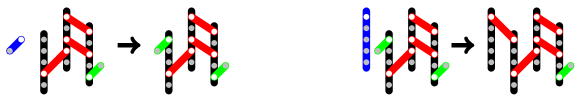
Figure 1: Left: Reaction 1: addition of a free cross-linker to the aggregate. Right: Reaction 2: addition of a p62₅ oligomer to the aggregate.

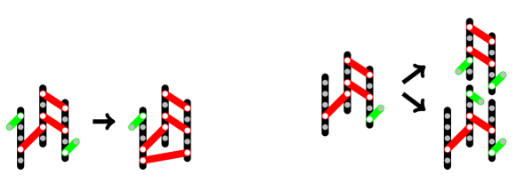
Figure 2: Left: Reaction 3 is a rearrangement making the aggregate more cohesive. Right: the breaking of a cross-link bound can lead either to the reverse of Reaction 2 of of Reaction 3.

Reaction 1 is the addition of a free cross-linker to the aggregate. This is a second order reaction with a rate proportional to the concentration of free cross-linkers and to the number of free binding sites on oligomers. Since the supply of free cross-linkers and oligomers has been modeled as not limiting in [1], the reaction rate is written as $\kappa_{1}(nr-p-2q)$ with rate constant $\kappa_{1}$, which can be seen as proportional to the cross-linker concentration, modeled as constant. Similarly Reaction 2, the addition of a free oligomer to the aggregate, is modeled as a first order reaction with rate $\kappa_{2}p$ proportional to the number of one-hand bound cross-linkers. Reaction 3 is consolidating the aggregate by building an additional cross-link using a so far only one-hand bound cross-linker. Its rate is $\kappa_{3}p(nr-p-2q)$. For the reverse of Reaction 1, the rate $\kappa_{-1}p$ should not be a surprise. The reverses of Reactions 2 and 3 are actually the same reaction with rate $\kappa_{-}q$, but with possibly different outcomes. Therefore we write their rate constants as $\kappa_{-2}:=\kappa_{-}\alpha$ and $\kappa_{-3}:=\kappa_{-}(1-\alpha)$, with $\alpha=\alpha(q,r)\in[0,1]$. The reverse of Reaction 2, i.e. loss of an oligomer, never happens in a fully connected aggregate with $nr=2q$. It always happens in a minimally connected aggregate with $q=r$. This motivates the choice $\alpha=\frac{nr-2q}{(n-2)r}$. Concerning the outcome of this reverse reaction, it has to be taken into account that the loss of an oligomer might also mean a loss of one-hand bound cross-links attached to it. This produces the loss term $\kappa_{-}q\frac{(n-1)p}{(n-2)r}$ (see [1] for details). It is now straightforward to write down the ODE problem governing the evolution of the state variables:

$$\dot{p} =(\kappa_{1}-\kappa_{3}p)(nr-p-2q)+\kappa_{-}q\left(1-\frac{(n-1)p}{(n-2)r}\right)-(\kappa_{2}+\kappa_{-1})p\,, \qquad p(0)=p_{0}\,,$$ (1)

$$\dot{q} =\kappa_{2}p+\kappa_{3}p(nr-p-2q)-\kappa_{-}q\,, \qquad q(0)=q_{0}\,,$$

$$\dot{r} =\kappa_{2}p-\kappa_{-}q\alpha(q,r),\qquad\alpha(q,r)=\frac{nr-2q}{(n-2)r}\,, \qquad r(0)=r_{0}\,,$$

with the inequalities

$$nr-p-2q\geq 0\,,\qquad q\geq r\,,$$ (2)

implying

$$0\leq\alpha(q,r)\leq 1\,.$$

We recall from [1, Theorem 1] that for initial data $p_{0},q_{0},r_{0}>0$ satisfying (2), which we assume in the following, the initial value problem (1) has a unique, global solution propagating (2), the nonnegativity of the components, and in particular

$$r(t),q(t)>0\,,\qquad t\geq 0\,.$$ (3)

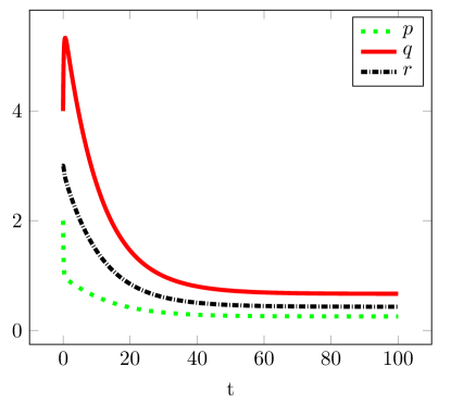
Figure 3: Evolution of a state $(p,q,r)$ of initial size $(2,4,3)$ with parameters $n=5$, $\kappa_{1}=\kappa_{2}=\kappa_{3}=\kappa_{-1}=1$, and $\kappa_{-}=0.6$, giving $0<\bar{\alpha}<1$ and convergence to the nontrivial equilibrium.

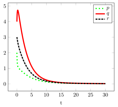
Figure 4: Evolution of a state $(p,q,r)$ of initial size $(2,4,3)$ with parameters $n=5$, $\kappa_{1}=\kappa_{2}=\kappa_{3}=\kappa_{-1}=1$ , and $\kappa_{-}=0.93$, giving $\bar{\alpha}>1$ and convergence to the zero steady state.

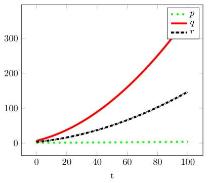
Figure 5: Evolution of a state $(p,q,r)$ of initial size $(2,4,3)$ with parameters $n=5$, $\kappa_{1}=\kappa_{2}=\kappa_{3}=\kappa_{-1}=1$, and $\kappa_{-}=0.2$, giving $\bar{\alpha}<0$ and a polynomially growing aggregate.

The search for steady states [1] has suggested a splitting of the parameter space into three regions. Besides the trivial steady state $(p,q,r)=(0,0,0)$, only one other equilibrium may exist, which can be computed explicitly:

$$\bar{p}=\frac{\kappa_{-}A}{\kappa_{2}}\frac{1-\bar{\alpha}}{\bar{\alpha}}\,,\qquad\bar{q}=A\frac{1-\bar{\alpha}}{\bar{\alpha}^{2}}\,,\qquad\bar{r}=\frac{2A}{n-(n-2)\bar{\alpha}}\frac{1-\bar{\alpha}}{\bar{\alpha}^{2}}\,,$$ (4)

$$\mbox{with}\quad\bar{\alpha}=\frac{n}{n-2}+\frac{\kappa_{-1}+\kappa_{1}-\sqrt{(\kappa_{1}+\kappa_{-1})^{2}+4\kappa_{1}\kappa_{2}(n-1)}}{\kappa_{-}(n-1)}\,,\quad A=\frac{2\kappa_{1}\kappa_{2}^{2}(n-2)}{\kappa_{3}\kappa_{-}(\kappa_{-}(n-1)(n-(n-2)\bar{\alpha})+2\kappa_{-1}(n-2))}\,.$$

Since $\bar{\alpha}=\alpha(\bar{q},\bar{r})$ is the equilibrium value of $\alpha$, the nontrivial steady state is relevant only in the parameter region defined by $0<\bar{\alpha}<1$. It has been conjectured in [1] that in this parameter region $(\bar{p},\bar{q},\bar{r})$ is globally attracting, which has been supported by numerical simulations (see also Fig. 3). Local stability could in principle be examined by linearization. However, the complexity of the resulting formulas has been prohibitive.

Since $(\bar{p},\bar{q},\bar{r})\to(0,0,0)$ as $\bar{\alpha}\to 1-$, it seems natural to expect a transcritical bifurcation at $\bar{\alpha}=1$ with stability of the trivial steady state for $\bar{\alpha}>1$. Again the conjecture of global asymptotic stability of $(0,0,0)$ for $\bar{\alpha}>1$ has been supported by simulations (see for example Fig. 4). The right hand sides of (1) are continuous up to the origin (when considered as an element of the set of admissible states), since $0\leq\alpha(q,r)\leq 1$ and $p/r\leq n$. However, their nonsmoothness prohibits a standard local stability or bifurcation analysis. The expected local stability behaviour (asymptotic stability for $\bar{\alpha}>1$, instability for $\bar{\alpha}<1$) is proven in Section 2. The analysis is based on a regularizing transformation, which makes the steady state very degenerate, combined with a blow-up analysis [2].

The fact that the components of the nontrivial equilibrium tend to infinity when $\bar{\alpha}\to 0+$ suggests that solutions might be unbounded for $\bar{\alpha}<0$. In this parameter region approximate solutions with polynomial growth of the form

$$p(t)=p_{1}t+\textit{o}(t)\,,\qquad q(t)=q_{2}t^{2}+\textit{o}(t^{2})\,,\qquad r(t)=\frac{2q_{2}}{n}t^{2}+\textit{o}(t^{2})\,,\qquad\mbox{as }t\to\infty\,,$$ (5)

have been constructed in [1] by formal asymptotic methods. It has also been shown that no other growth behaviour (polynomial with other powers or exponential) should be expected, and the conjecture that all solutions have the constructed asymptotic behaviour is again verified by simulations (see Fig. for example 5). We justify the formal asymptotics in Section 3. A variant of Poincaré compactification [4] produces a problem with bounded solutions and with three different time scales, which is analyzed by singular perturbation methods [3]. The final result is existence and semi-local stability of the polynomially growing solutions, where ’semi-local’ means that initial data have to be large with relative sizes as in (5).

The article is concluded by a discussion section about biological interpretation of our results as well as perspectives.

2 Local stability of the zero steady state

In this section, we study under which conditions small aggregates tend to disaggregate. This is equivalent to studying the stability of the zero-steady-state $(p,q,r)=(0,0,0)$ of the system (1). Because of the appearance of the ratios $\frac{p}{r}$ and $\frac{q}{r}$, the Jacobian of the right hand side of (1) is not defined there. As a consequence of (3) the regularizing transformation $\tau:=\int_{0}^{t}r(s)^{-1}\mathrm{d}s$ is well defined and leads to

$$\frac{dp}{d\tau} =r(\kappa_{1}-\kappa_{3}p)(nr-p-2q)+\kappa_{-}q\left(r-\frac{(n-1)p}{n-2}\right)-(\kappa_{2}+\kappa_{-1})pr\,,$$ (6)

$$\frac{dq}{d\tau} =\kappa_{2}pr+\kappa_{3}pr(nr-p-2q)-\kappa_{-}qr\,,$$

$$\frac{dr}{d\tau} =\kappa_{2}pr-\kappa_{-}q\frac{nr-2q}{n-2}\,.$$

The regularization came at the expense that the zero steady state is degenerate in (6), since the right hand side is of second order in terms of the densities. A classical approach to study such non-hyperbolic points is blow-up [2]. The standard blow-up transformation would be the introduction of spherical coordinates, blowing up the origin to the part of $\mathbb{S}^{2}$ in the positive octant. It is also common to work with charts instead. In our case this preserves the polynomial form of the right hand side. Although the charts in the different coordinate directions are equivalent, since the state space is a subset of the positive octant, it has turned out to be convenient to use the $q$-chart, whence the blow-up transformation $(p,q,r)\to(p_{1},q_{1},r_{1})$ is given by

$$p=p_{1}q_{1}\,,\qquad q=q_{1}\,,\qquad r=r_{1}q_{1}\,,$$ (7)

and we also introduce another change of time scale: $T:=\int_{0}^{\tau}q_{1}(\sigma)d\sigma$, again justified by (3), leading to

$$\frac{dq_{1}}{dT} = q_{1}r_{1}\left(\kappa_{2}p_{1}-\kappa_{-}\right)+\kappa_{3}p_{1}r_{1}q_{1}^{2}(nr_{1}-p_{1}-2)\,,$$

$$\frac{dp_{1}}{dT} = r_{1}(\kappa_{1}-\kappa_{3}p_{1}q_{1})(nr_{1}-p_{1}-2)+\kappa_{-}\left(r_{1}-\frac{n-1}{n-2}p_{1}\right)-(\kappa_{2}+\kappa_{-1})p_{1}r_{1}-p_{1}r_{1}(\kappa_{2}p_{1}-\kappa_{-})$$ (8)

$$-\kappa_{3}p_{1}^{2}r_{1}q_{1}(nr_{1}-p_{1}-2)\,,$$

$$\frac{dr_{1}}{dT} = (1-r_{1})\left(\kappa_{2}p_{1}r_{1}+\kappa_{-}\left(\frac{2}{n-2}-r_{1}\right)\right)-\kappa_{3}p_{1}r_{1}^{2}q_{1}(nr_{1}-p_{1}-2)\,.$$

The invariant manifold $q_{1}=0$ of this system corresponds to the zero steady state of (1). The inequalities (2) become

$$r_{1}\leq 1\,,\qquad 0\leq p_{1}\leq nr_{1}-2\,,$$

in terms of the new variables, i.e. the dynamics of $(p_{1},r_{1})$ remains in the triangle depicted in Fig. 6. Since $r_{1}\geq 2/n$, we conclude from the equation for $q_{1}$ that the invariant manifold is locally exponentially attracting in the region to the left of the line $p_{1}=\kappa_{-}/\kappa_{2}$. Since $p_{1}\leq n-2$, the inequality $\kappa_{-}>(n-2)\kappa_{2}$ already implies local asymptotic stability of the invariant manifold $q_{1}=0$ of (8) and therefore of the zero steady state of (1). Note that $\kappa_{-}>(n-2)\kappa_{2}$ also implies $\bar{\alpha}>1$ for $\bar{\alpha}$ defined by (4).

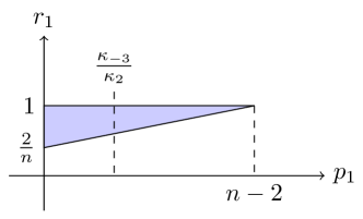
Figure 6: The dynamics in the $(p_{1},r_{1})$-plane is limited to the shaded triangle because of the inequalities (2).

In the following we therefore consider the case $\kappa_{-}\leq(n-2)\kappa_{2}$ (see Fig. 6) and $\bar{\alpha}>1$, where the latter is equivalent to

$$\kappa_{1}\kappa_{2}(n-2)^{2}<\kappa_{-}(\kappa_{1}+\kappa_{-1})(n-2)+\kappa_{-}^{2}(n-1)\,,$$ (9)

see also [1, Equ. (26)]. The flow on the invariant manifold $q_{1}=0$ of (8) is governed by the system

$$\frac{dp_{1}}{dT} = r_{1}\kappa_{1}(nr_{1}-p_{1}-2)+\kappa_{-}\left(r_{1}-\frac{n-1}{n-2}p_{1}\right)-(\kappa_{2}+\kappa_{-1})p_{1}r_{1}-p_{1}r_{1}(\kappa_{2}p_{1}-\kappa_{-})$$

$$\frac{dr_{1}}{dT} = (1-r_{1})\left(\kappa_{2}p_{1}r_{1}+\kappa_{-}\left(\frac{2}{n-2}-r_{1}\right)\right)\,.$$ (10)

In the right part of the triangle, i.e. for

$$r_{1}\leq 1\,,\qquad\frac{\kappa_{-}}{\kappa_{2}}\leq p_{1}\leq nr_{1}-2\,,$$

we have

$$\frac{dp_{1}}{dT} \leq r_{1}\kappa_{1}\left(n-\frac{\kappa_{-}}{\kappa_{2}}-2\right)+\kappa_{-}\left(r_{1}-\frac{n-1}{n-2}\,\frac{\kappa_{-}}{\kappa_{2}}\right)-(\kappa_{2}+\kappa_{-1})\frac{\kappa_{-}}{\kappa_{2}}r_{1}$$

$$= \frac{r_{1}\bigl{(}\kappa_{1}\kappa_{2}(n-2)^{2}-\kappa_{-}(\kappa_{1}+\kappa_{-1})(n-2)\bigr{)}-\kappa_{-}^{2}(n-1)}{\kappa_{2}(n-2)}<\frac{(r_{1}-1)\kappa_{-}^{2}(n-1)}{\kappa_{2}(n-2)}\leq 0\,,$$

where the strict inequality is due to (9). This implies that all trajectories reach the left part of the triangle, i.e. $p_{1}<\kappa_{-}/\kappa_{2}$ in finite time.

By standard regular perturbation theory the dynamics for the full system (8), when started close to the invariant manifold $q_{1}=0$, remains close to the dynamics on the invariant manifold for finite time, until the region $p_{1}<\kappa_{-}/\kappa_{2}$ is reached, where the invariant manifold is attracting. Thus $q=q_{1}$ tends to zero and, by the inequalities (2), the same is true for $p$ and $r$.

Now we consider the case $\bar{\alpha}<1$, i.e. the opposite of inequality (9), and look for a steady state on the invariant manifold $r_{1}=1$ of the system (10). Since

$$\frac{dp_{1}}{dT}\Bigm{|}_{r_{1}=1,p_{1}=\kappa_{-}/\kappa_{2}} = \frac{\kappa_{1}\kappa_{2}(n-2)^{2}-\kappa_{-}(\kappa_{1}+\kappa_{-1})(n-2)-\kappa_{-}^{2}(n-1)}{\kappa_{2}(n-2)}>0\,,$$

$$\frac{dp_{1}}{dT}\Bigm{|}_{r_{1}=1,p_{1}=n-2} = -(n-2)(n\kappa_{2}+\kappa_{-1})<0\,,$$

there exists a steady state $(p_{1},r_{1})=(p_{1}^{*},1)$ with $\kappa_{-}/\kappa_{2}<p_{1}^{*}<n-2$, which is stable under the flow along $r_{1}=1$. On the other hand

$$\frac{1}{1-r_{1}}\,\frac{dr_{1}}{dT}\Bigm{|}_{r_{1}=1,p_{1}=p_{1}^{*}}=\left(\kappa_{2}p_{1}^{*}+\kappa_{-}\left(\frac{2}{n-2}-1\right)\right)>\frac{2\kappa_{-}}{n-2}>0\,,$$

which implies stability of the manifold $r_{1}=1$ close to the steady state, and therefore stability of the steady state. The existence of a stable steady state on the invariant manifold $q_{1}=0$ of (8) in the region, where the manifold is repulsive, implies instability of the manifold and therefore also of the zero steady state of (1). This completes the proof of the main result of this section.

Theorem 1.

Let $\bar{\alpha}$ be defined by (4). Then the steady state $(0,0,0)$ of the system (1) is locally asymptotically stable for $\bar{\alpha}>1$ and unstable for $\bar{\alpha}<1$.

3 Polynomially growing regime

The goal of this section is a rigorous justification of the formal asymptotics (5) (see [1]) under the assumption $\bar{\alpha}<0$ with $\bar{\alpha}$ defined in (4), i.e.

$$4\kappa_{1}\kappa_{2}(n-2)^{2}>n\kappa_{-}\bigl{(}2(\kappa_{1}+\kappa_{-1})(n-2)+\kappa_{-}n(n-1)\bigr{)}\,,$$ (11)

see also [1, Equ. (27)].

Considering (5), it would be natural to write an equation for $p(t)/t$. It is easily seen from (1) that its derivative contains terms of the order of $t^{2}$. Similarly the derivative of $q(t)/t^{2}$ has contributions up to the order of $t$, whereas the derivative of $r(t)/t^{2}$ is a combination of terms bounded as $t\to\infty$. This shows that we are confronted with a problem with different time scales, which will put us into the realm of singular perturbation theory (see, e.g. [3, 6]). The leading order term in the fastest equation, i.e. the $p$-equation, is $-\kappa_{3}p(nr-2q)$, from which it has been concluded in [1] that $nr(t)\approx 2q(t)$ as $t\to\infty$. In a standard singular perturbation setting, it should be possible to express $p(t)$ from this relation. Since this is not the case, our problem belongs to the family of singular singularly perturbed problems (see e.g. [5]) which, however, can be transformed to the standard regular form in many cases.

The introduction of $p(t)/t$, $q(t)/t^{2}$, $r(t)/t^{2}$, as new variables would lead to a study of bounded solutions, but to a non-autonomous system. We shall use a variant of the Poincaré compactification method [4] instead.

The previous observations led us to the introduction of the new variables

$$u=\frac{p}{\sqrt{p+q}}\,,\qquad v=\frac{2p+2q-nr}{\sqrt{p+q}}\,,\qquad w=\frac{1}{\sqrt{p+q}}\,,$$

where we expect that $w(t)$ tends to zero as $t^{-1}$, and that $u(t)$ and $v(t)$ converge to nontrivial limits. Since this coordinate change produces a singularity at $w=0$, we also change the time variable by $\tau=\int_{0}^{t}ds/w(s)$. In terms of the new variables system (1) becomes

$$\frac{du}{d\tau} = (\kappa_{1}w-\kappa_{3}u)(u-v)+\kappa_{-}(1-uw)\left(1-\frac{n(n-1)uw}{(n-2)(2-vw)}\right)-(\kappa_{2}+\kappa_{-1})uw$$

$$-uw^{2}A(u,v,w)\,,$$

$$\frac{dv}{d\tau} = w\left(2\kappa_{1}(u-v)-(2\kappa_{-1}+n\kappa_{2})u+\kappa_{-}(1-uw)n\frac{2u-nv}{(n-2)(2-vw)}\right)-vw^{2}A(u,v,w)\,,$$ (12)

$$\frac{dw}{d\tau} = -w^{3}A(u,v,w)\,,\quad A(u,v,w):=\frac{1}{2}\left(\kappa_{1}(u-v)-\kappa_{-1}u-\kappa_{-}(1-uw)\frac{n(n-1)u}{(n-2)(2-vw)}\right)\,.$$

Our goal is to prove that solutions converge to a steady state $(u^{*},v^{*},w^{*})$ with $w^{*}=0$, which obviously has to satisfy $-\kappa_{3}u^{*}(u^{*}-v^{*})+\kappa_{-}=0$, implying

$$u^{*}=U(v^{*}):=\frac{1}{2}\left(v^{*}+\sqrt{(v^{*})^{2}+4\kappa_{-}/\kappa_{3}}\right)\,,$$ (13)

since we need $u^{*}>0$. We intend to show that $v^{*}$ is determined from the requirement that the large parenthesis in the $v$-equation vanishes. The argument is essentially that for small values of $w$, the variable $v$ evolves much faster than $w$.

In order to make the slow-fast structure of this system more apparent and to allow the application of basic results from singular perturbation theory, we assume that the initial value for $w$ is small and define $\varepsilon:=(p_{0}+q_{0})^{-1/2}\ll 1$ and the rescaled variable $W=w/\varepsilon$, leading to

$$\frac{du}{d\tau} = -\kappa_{3}u(u-v)+\kappa_{-}+O(\varepsilon)\,,$$

$$\frac{dv}{d\tau} = \varepsilon W\left(2\kappa_{1}(u-v)-(2\kappa_{-1}+n\kappa_{2})u+\kappa_{-}n\frac{2u-nv}{2(n-2)}\right)+O(\varepsilon^{2})\,,$$ (14)

$$\frac{dW}{d\tau} = -\varepsilon^{2}W^{3}A(u,v,0)+O(\varepsilon^{3})\,.$$

The initial data are denoted by

$$u(0)=u_{0}:=\frac{p_{0}}{\sqrt{p_{0}+q_{0}}}>0\,,\qquad v(0)=v_{0}:=\frac{2p_{0}+2q_{0}-nr_{0}}{\sqrt{p_{0}+q_{0}}}\,,\qquad W(0)=1\,,$$

where in the following we consider $u_{0}$ and $v_{0}$ as fixed when $\varepsilon\to 0$. This is a singular perturbation problem in standard form, where $\tau$ plays the role of an initial layer variable. We pass to the limit $\varepsilon\to 0$ to obtain the initial layer problem

$$\frac{d\hat{u}}{d\tau} = -\kappa_{3}\hat{u}(\hat{u}-\hat{v})+\kappa_{-}\,,$$ (15)

$$\frac{d\hat{v}}{d\tau} = \frac{d\hat{W}}{d\tau}=0\,,$$

subject to the initial conditions. By the qualitative behaviour of the right hand side of the first equation, the solution satisfies $\hat{v}(\tau)=v_{0}$, $\hat{W}(\tau)=1$, and

$$\lim_{\tau\to\infty}\hat{u}(\tau)=U(v_{0})\,,$$

with exponential convergence, where $U$ has been defined in (13). The equation $u=U(v)$ defines the so called reduced manifold. Since it is exponentially attracting, the Tikhonov theorem [7] (or rather its extension [3]) implies that, after the initial layer, i.e. when written in terms of the slow variable $\sigma=\varepsilon\tau$, the solution trajectory remains exponentially close to the slow manifold, which is approximated by the reduced manifold, and the flow on the slow manifold satisfies

$$\frac{dv}{d\sigma} = W\left(2\kappa_{1}(U(v)-v)-(2\kappa_{-1}+n\kappa_{2})U(v)+\kappa_{-}n\frac{2U(v)-nv}{2(n-2)}\right)+O(\varepsilon)\,,$$

$$\frac{dW}{d\sigma} = -\varepsilon W^{3}A(U(v),v,0)+O(\varepsilon^{2})\,,$$ (16)

with $v(0)=v_{0}$, $W(0)=1$. This is again a singular perturbation problem in standard form, where now $\sigma$ is the initial layer variable. We repeat the above procedure and consider the limiting layer problem

$$\frac{d\tilde{v}}{d\sigma} = \tilde{W}\left(2\kappa_{1}(U(y\tilde{v})-\tilde{v})-(2\kappa_{-1}+n\kappa_{2})U(\tilde{v})+\kappa_{-}n\frac{2U(\tilde{v})-n\tilde{v}}{2(n-2)}\right)\,,$$ (17)

$$\frac{d\tilde{W}}{d\sigma} = 0\,.$$

The observations

$$U(-\infty)=0\,,\qquad U(\infty)=\infty\,,\qquad 0<U^{\prime}(v)<1\,,$$

suffice to show that the right hand side of the first equation is a strictly decreasing function of $v$ with a unique zero $v^{*}$, which can actually be computed explicitly:

$$v^{*}=B\left(\kappa_{1}-\kappa_{-1}-\frac{n}{2}\kappa_{2}+\frac{n}{2(n-2)}\kappa_{-}\right)$$

$$\mbox{with}\quad B=2\sqrt{\frac{\kappa_{-}}{\kappa_{3}}}\left(\frac{n^{3}}{4(n-2)}\kappa_{-}^{2}+4\kappa_{1}\kappa_{-1}+2n\kappa_{1}\kappa_{2}+n\kappa_{1}\kappa_{-}+\frac{n^{2}}{n-2}\kappa_{-1}\kappa_{-}+\frac{n^{3}}{2(n-2)\kappa_{2}\kappa_{-}}\right)^{-1/2}$$

The solution of (17) with $\tilde{v}(0)=v_{0}$ satisfies $\lim_{\sigma\to\infty}\tilde{v}(\sigma)=v^{*}$ with exponential convergence. Another application of the Tikhonov theorem shows that the slowest part of the dynamics with $t=O(\varepsilon^{-1})$ can be approximated by

$$\frac{dW}{d\sigma}=-\varepsilon W^{3}A^{*}\,,\qquad W(0)=1\,,$$ (18)

with

$$A^{*}:=A(U(v^{*}),v^{*},0)=\frac{nB}{16(n-2)^{2}}(4(n-2)^{2}\kappa_{1}\kappa_{2}-2n(n-2)\kappa_{-}(\kappa_{1}+\kappa_{-1})-n^{2}(n-1)\kappa_{-}^{2})>0\,,$$ (19)

by (11). This gives the approximation

$$W(\sigma)=(1+2A^{*}\varepsilon\sigma)^{-1/2}\,.$$

The results of [3] imply that the approximations are accurate with errors of order $\varepsilon$ uniformly with respect to time.

Theorem 2.

Let (11) hold. Then, for $\varepsilon>0$ small enough, the solution of (12) with initial conditions

$$u(0)=u_{0}>0\,,\qquad v(0)=v_{0}\in\mathbb{R}\,,\qquad w(0)=\varepsilon\,,$$

satisfies

$$u(\tau) = \hat{u}(\tau)-U(v_{0})+U(\tilde{v}(\varepsilon\tau))+O(\varepsilon)\,,$$

$$v(\tau) = \tilde{v}(\varepsilon\tau)+O(\varepsilon)\,,$$

$$w(\tau) = \varepsilon(1+2A^{*}\varepsilon^{2}\tau)^{-1/2}+O(\varepsilon^{2})\,,$$

uniformly in $\tau\geq 0$, where $U$ is given in (13), $\hat{u}$ solves (15), $\tilde{v}$ solves (17), and $A^{*}$ is given in (19).

Actually more can be deduced. In terms of the original time variable $t$, the equation for $w$ in (12) becomes

$$\dot{w}=-w^{2}A(u,v,w)\,.$$ (20)

Under the assumptions of Theorem 2, $A(u,v,w)$ is uniformly close to the positive constant $A^{*}$ and therefore uniformly positive for large enough $t$. This implies that $w$ tends to zero as $t\to\infty$. The slow manifold of the system (16) reduces to the steady state $(v,W)=(v^{*},0)$ for $W=0$. Therefore $v$ tends to $v^{*}$ as $t\to\infty$. Analogously, the slow manifold of (14) reduces to the steady state $(u,v,W)=(u^{*}=U(v^{*}),v^{*},0)$ at $W=0$, implying convergence of $u$ to $u^{*}$. This in turn implies convergence of $A(u,v,w)$ to $A^{*}$, which can be used in (20).

Corollary 1.

Let the assumptions of Theorem 2 hold. Then

$$\lim_{t\to\infty}u(t)=u^{*}\,,\qquad\lim_{t\to\infty}v(t)=v^{*}\,,\qquad w(t)=\frac{1}{A^{*}t}+O\left(\frac{1}{t^{2}}\right)\quad\mbox{as }t\to\infty\,.$$

Finally, we reformulate these results in terms of the original variables, verifying the formal asymptotics of [1] for initial data, which are in a sense already ’close enough’ to the polynomially growing solutions.

Theorem 3.

Let (11) hold, let $c_{2}\geq c_{1}>0$, and let $\delta>0$ be small enough. Let the initial data satisfy

$$p_{0}=\frac{c_{1}}{\delta}\,,\qquad q_{0}=\frac{1}{\delta^{2}}\,,\qquad r_{0}=\frac{2}{n\delta^{2}}+\frac{c_{2}}{n\delta}$$

Then the solution of (1) with $(p(0),q(0),r(0))=(p_{0},q_{0},r_{0})$ satisfies

$$p(t)=u^{*}A^{*}t+o(t)\,,\qquad q(t)=(A^{*})^{2}t^{2}+o(t^{2})\,,\qquad r(t)=\frac{2}{n}(A^{*})^{2}t^{2}+o(t^{2})\,,\qquad\mbox{as }t\to\infty\,.$$

Proof.

We just need to verify that the assumptions of this theorem imply the assumptions of Theorem 2. The result is then a direct consequence of Corollary 1. Actually the assumptions of Theorem 2 hold with $\varepsilon\approx\delta$, since

$$u_{0}=\frac{c_{1}}{\sqrt{1+c_{1}\delta}}\,,\qquad v_{0}=\frac{2c_{1}-c_{2}}{\sqrt{1+c_{1}\delta}}\,,\qquad w_{0}=\frac{\delta}{\sqrt{1+c_{1}\delta}}\,.$$

∎

4 Discussion

In this work a mathematical model for aggregation via cross-linking has been analyzed. Besides the basic assumption that aggregating particles (here p62 oligomers) need to have at least $n=3$ binding sites for cross-linkers (here ubiqutinated cargo), the rate constants for binding reactions need to be large enough compared to those for the unbinding reactions (the opposite of inequality (9)) for stable aggregates to exist. Under a stronger condition (inequality (11)) aggregates grow indefinitely in the presence of an unlimited supply of free particles and cross-linkers. These conjectures from [1], where the model has been formulated, have been partially proven in this work. It has been shown in Section 2 that small aggregates get completely degraded under the condition (9) and that they grow under the opposite condition. In the latter case, but when (11) does not hold, there exists an equilibrium configuration with positive aggregate size. Finally, it has been shown in Section 3 that under the condition (11) aggregate size grows polynomially with time (actually like $t^{2}$) for appropriate initial states.

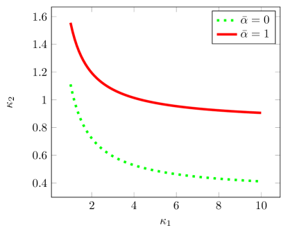
Figure 7: Bifurcation diagram obtained for $\kappa_{-1}=\kappa_{-}=1$

The constants $\kappa_{1}$, $\kappa_{2}$ in the model have to be interpreted as the products of rate constants with the concentrations of free cross-linkers and, respectively, of free particles. This means that the conditions (9) and (11) are actually conditions for these concentrations. Fig. 7 shows a bifurcation diagram in terms of $\kappa_{1}$ and $\kappa_{2}$ with the curves $\bar{\alpha}=1$, corresponding to equality in (9), and $\bar{\alpha}=0$, corresponding to equality in (11). The qualitative behaviour is no surprise: Close to the origin, i.e. for small concentrations of free particles and cross-linkers, aggregates are unstable. Moving to the right and/or up we pass through two bifurcations to stable finite aggregate size and, subsequently, to polynomial growth of aggregates. Less obvious is the fact that the picture is rather unsymmetric with respect to the two parameters. The condition $(n-2)\kappa_{2}>\kappa_{-}$ is necessary for the existence of stable aggregates, regardless of the value of $\kappa_{1}$, whereas arbitrarily small values of $\kappa_{1}$ can be compensated by large enough $\kappa_{2}$. This means that, if the concentration of free particles is below a threshold, even a large concentration of cross-linkers does not lead to aggregation, whereas arbitrarily small numbers of cross-linkers are used for aggregation if the particle concentration is high. For the application in cellular autophagy this means that aggregation will only happen for large enough concentrations of p62 oligomers. However, arbitrarily small amounts of ubiquitinated cargo can be aggregated in the presence of a large enough supply of oligomers.

This work has been motivated by the experimental results of [8], where aggregates have been detected by light microscopy. If the evolution of single aggregates can be followed, the growth like $t^{2}$ might be observed as a fluorescence signal of tagged oligomers, which goes like $t^{2}$, or cross section areas going like $t^{4/3}$, if a roughly spherical shape of aggregates is assumed. For quantitative predictions of such experiments, the model should be extended in various ways. First, the limited supply of free p62 oligomers and of free cross-linkers should be taken into account. This is straightforward for the modeling of a single aggregate, but if many aggregates develop simultaneously, they will compete for the free particles. Apart from that the number of aggregates has to be predicted, which requires modeling of the nucleation process. Finally, it is very likely that the coagulation of aggregates plays an important role. A growth-coagulation model for distributions of aggregates, based on the growth model (1) would be prohibitively complex. It is therefore the subject of ongoing work to formulate, analyze, and simulate a growth-coagulation model based on the multiscale analysis of Section 3, where aggregates are only described by the size parameter $r$ (number of p62 oligomers in the aggregate), whose evolution is determined by the slow dynamics (18), which translates to an equation of the form $\dot{r}=C\sqrt{r}$ for $r$. This approach raises several challenging issues such as the development of an efficient simulation algorithm or the existence and stability of equilibrium aggregate distributions.

References

[1]
J. Delacour, M. Doumic, S. Martens, C. Schmeiser, and G. Zaffagnini.
A mathematical model of p62-ubiquitin aggregates in autophagy.
arXiv:2004.07926.
[2]
F. Dumortier.
Techniques in the theory of local bifurcations: Blow-up, normal
forms, nilpotent bifurcations, singular perturbations.
In Bifurcations and Periodic Orbits of Vector Fields, pages
19–73. Kluwer Acad. Publ., 1993.
[3]
N. Fenichel.
Geometric singular perturbation theory for ordinary differential
equations.
Journal of Differential Equations, 31:53–98, 1979.
[4]
H. Poincaré.
Mémoire sur les courbes définies par une équation
différentielle (i).
Journal de mathématiques pures et appliquées 3e série,
tome 7, pages 375–422, 1881.
[5]
C. Schmeiser and R. Weiß.
Asymptotic analysis of singular singularly perturbed boundary value
problems.
SIAM J. Math. Anal., 17:560–579, 1986.
[6]
P. Szmolyan.
Transversal heteroclinic and homoclinic orbits in singular
perturbation problems.
Journal of Differential Equations, 92:252–281, 1991.
[7]
A. N. Tikhonov.
Systems of differential equations containing small parameters in the
derivatives.
Matematicheskii sbornik, 73:575–586, 1952.
[8]
G. Zaffagnini, A. Savova, A. Danieli, J. Romanov, S. Tremel, M. Ebner,
T. Peterbauer, M. Sztacho, R. Trapannone, A.K. Tarafder, C. Sachse, and
S. Martens.
p62 filaments capture and present ubiquitinated cargos for autophagy.
The EMBO Journal, 37(5):e98308, 03 2018.