Rigid and Articulated Point Registration with Expectation Conditional Maximization

Abstract

This paper addresses the issue of matching rigid and articulated shapes through probabilistic point registration. The problem is recast into a missing data framework where unknown correspondences are handled via mixture models. Adopting a maximum likelihood principle, we introduce an innovative EM-like algorithm, namely the Expectation Conditional Maximization for Point Registration (ECMPR) algorithm. The algorithm allows the use of general covariance matrices for the mixture model components and improves over the isotropic covariance case. We analyse in detail the associated consequences in terms of estimation of the registration parameters, and we propose an optimal method for estimating the rotational and translational parameters based on semi-definite positive relaxation. We extend rigid registration to articulated registration. Robustness is ensured by detecting and rejecting outliers through the addition of a uniform component to the Gaussian mixture model at hand. We provide an in-depth analysis of our method and we compare it both theoretically and experimentally with other robust methods for point registration.

I Introduction, related work, and contributions

In image analysis and computer vision there is a long tradition of algorithms for finding an optimal alignment between two sets of points. This is referred to as the point registration (PR) problem, which is twofold: (i) Find point-to-point correspondences and (ii) estimate the transformation allowing the alignment of the two sets. Existing PR methods can be roughly divided into three categories: The Iterative Closest Point (ICP) algorithm [1, 2] and its numerous extensions [3, 4, 5, 6, 7, 8], soft assignment methods [9, 10, 11, 12], and probabilistic methods [13, 14, 15, 16, 17, 18] to cite just a few.

ICP alternates between binary point-to-point assignments and optimal estimation of the transformation parameters. Efficient versions of ICP use sampling processes, either deterministic or based on heuristics [3]. Sampling strategies can be cast into more elaborate outlier rejection methods such as [4] which applies a robust loss function to the Euclidean distance, thus yielding a non-linear version of ICP called LM-ICP. Another standard robust method is to select trimmed subsets of points through repeated random sampling, such as the TriICP algorithm proposed in [5]. In [6] a maximum-likelihood non-linear optimizer is bootstrapped by combining ICP with a RANSAC-like trimming method [19]. Although ICP is attractive for its efficiency, it can be easily trapped in local minima due to the strict selection of the best point-to-point assignments. This makes ICP to be particularly sensitive both to initialization and to the choice of a threshold needed to accept or to reject a match.

The nearest-point strategy of ICP can be replaced by soft assignments within a continuous optimization framework [9, 10]. Let $m_{ji}$ be the positive entries of the assignment matrix $\mathbf{M}$, subject to the constraints $\sum_{j}m_{ji}=1$, $\sum_{i}m_{ji}=1$. When there is an equal number of points in the two sets, $\mathbf{M}$ is a doubly stochastic matrix. This introduces nonconvex constraints: Indeed, the PR problem is solved using Lagrange parameters and a barrier function within a constrained optimization approach [9]. The RPM algorithm [10] extends [9] to deal with outliers. This is done by adding one column and one row to matrix $\mathbf{M}$, say $\widetilde{\mathbf{M}}$. Several data points are allowed to be assigned to this extra column and, symmetrically, several model points may be assigned to this extra row. Therefore, the resulting algorithm must provide optimal entries for $\widetilde{\mathbf{M}}$ and satisfy the constraints on $\mathbf{M}$, thus providing one-to-one assignments for inliers, and many-to-one assignments for outliers, i.e., several entries are allowed to be equal to 1 in both the extra row and the extra column. As a consequence, $\widetilde{\mathbf{M}}$ is not doubly stochastic anymore and hence the convergence properties as described in [20] are not guaranteed in the presence of outliers.

Probabilistic point registration uses, in general, Gaussian mixture models (GMM). Indeed, one may reasonably assume that points from the first set (the data) are normally distributed around points belonging to the second set (the model). Therefore, the point-to-point assignment problem can be recast into that of estimating the parameters of a mixture. This can be done within the framework of maximum likelihood with missing data because one has to estimate the mixture parameters as well as the point-to-cluster assignments, i.e., the missing data. In this case the algorithm of choice is the expectation-maximization (EM) algorithm [21]. Formally, the latter replaces the maximization of the observed-data log-likelihood with the maximization of the expected complete-data log-likelihood conditioned by the observations. As it will be explained in detail in this paper, there are intrinsic difficulties when one wants to cast the PR problem in the EM framework. The main topic and contribution of this paper is to propose an elegant and efficient way to do that.

In the recent past, several interesting EM-like implementations for point registration have been proposed [13, 14, 15, 16]. In [13] the posterior marginal pose estimation (PMPE) method estimates the marginalized joint posterior of alignment and correspondence over all possible correspondences. This formulation does not lead to the standard M-step of EM and, in particular, it does not allow the estimation of the covariances of the Gaussian mixture components. The complete-data posterior energy function is used in [14]. This leads to an E-step which updates a set of continuous assignment variables which are similar but not identical to the standard posterior probabilities of assigning points to clusters [22]. It also leads to an M-step which involves optimization of a non-linear energy function which is approximated for simplification. The algorithms proposed in [13] and [14] do not lead to the true maximum-likelihood (ML) solution.

In [14] as well as in [15] and [16] a simplified GMM is used, namely a mixture with a spherical (isotropic) covariance common to all the components. This has two important consequences. First, it significantly simplifies the estimation of the alignment parameters because the Mahalanobis distance is replaced by the Euclidean distance: this allows the use of a closed-form solution to find the optimal rotation matrix [23, 24, 25, 26], as opposed to an iterative numerical solution as proposed in [27]. Second, it allows connections between GMM, EM, and deterministic annealing [28]: The common variance is interpreted as a temperature and its value is decreased at each step of the algorithm according to an annealing schedule [9, 10, 14, 15, 16]. Nevertheless, the spherical-covariance assumption inherent to annealing has a number of drawbacks: anisotropic noise in the data is not properly handled, it does not use the full Gaussian model, and it does not fully benefit from the convergence properties of EM because it anneals the variance rather than considering it as a parameter to be estimated.

Another approach is to model each one of the two point sets by two probability distributions and to measure the dissimilarity between the two distributions [29, 30, 18, 31]. For example, in [18], each point set is modelled by a GMM where the number of components is chosen to be equal to the number of points. In the case of rigid registration, this is equivalent to replace the quadratic loss function with a Gaussian and to minimize the sum of these Gaussians over all possible point pairs. The Gaussian acts as a robust loss function. However there are two major drawbacks: The formulation leads to a non-linear optimization problem which must be solved under the nonconvex rigidity constraints, which require proper initialization. Second, the outliers are not explicitly modeled.

This paper has the following original contributions:

• We formally cast the PR problem into the framework of maximum likelihood with missing data. We derive a maximization criterion based on the expected complete-data log-likelihood. We show that, within this context, the PR problem can be solved by an instance of the the expectation conditional maximization (ECM) algorithm. It has been proven that ECM is more broadly applicable than EM while it shares its desirable convergence properties [32]. In ECM, each M-step is replaced by a sequence of conditional maximization steps, or CM-steps. As it will be explained and detailed in this paper, ECM is particularly well suited for point registration because the maximization over the registration parameters cannot be carried out independently of the other parameters of the model, namely the covariances. For these reasons we propose the Expectation Conditional Maximization for Point Registration algorithm (ECMPR).

• The vast majority of existing rigid point registration methods use isotropic covariances for reasons that we just explained. In the more general case of anisotropic covariances, we show that the optimization problem associated with rigid alignment cannot be solved in closed-form. The iterative numerical solution proposed in [27] estimates the motion parameters without estimating the covariances. We propose and devise a novel solution to this problem which consists in transforming the nonconvex problem into a convex one using semi-definite positive (SDP) relaxation [33]. Hence, rigid alignment in the presence of anisotropic covariance matrices is amenable to a tractable optimization problem.

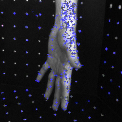
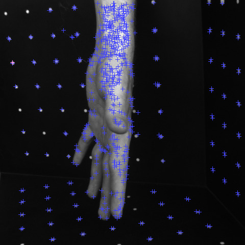
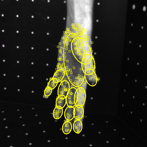
  Figure 1: An illustration of the point registration method applied to the problem of aligning an articulated model of a hand to a set of 3D points. The 3D data are obtained by stereo reconstruction from an image pair (top). The hand model consists of 3D points lying on 16 hand parts (one root part, i.e., the palm, and 3 additional parts for each finger). The model contains 5 kinematic chains, each one is composed of the palm and one finger, i.e., 4 parts. Hence, the palm, or the root part, is common to all the kinematic chains. This articulated model has 27 degrees of freedom (3 translations and 3 rotations for the palm, 5 rotations for the thumb and 4 rotations for the index, middle, ring, and baby fingers). The result of the ECMPR-articulated algorithm is shown projected onto the left image (bottom-left) and as an implicit surface defined as a blending over the 16 hand parts (bottom-right).

• We extend the rigid alignment solution just mentioned to articulated alignment. Based on the fact that the kinematic motion of an articulated object can be written as a chain of constrained rigid motions, we devise an incremental solution which iteratively applies the rigid-alignment solution just mentioned to the rigid parts of the kinematic chain. There are a few methods for aligning articulated objects via point registration. In [7] ICP is first applied independently to each rigid part of the articulated object and next, the articulated constraints are enforced. The articulated ICP method of [8] alternates between associating points from the two sets and estimating the articulated pose. The latter is done by minimizing a non-linear least-square error function which ensures that the rigid body parts are in an optimal pose while the kinematic joint constraints are only weakly satisfied. Our approach has two advantages with respect to these methods. First, rather than ICP, we use ECM which has proven convergence properties and which can handle inliers and outliers in a principled way. Second, our incremental rigid alignment formulation naturally enforces the kinematic constraints. As a consequence, these constraints hold exactly and there is no need to enforce them a posteriori. Moreover, the articulated registration method that we propose takes full advantage of the rigid point registration algorithm, which is quite different from data-point-to-object-part registration [34, 35, 36, 37, 38]. We note that our method is similar in spirit with [39]. However, the latter suffers from the limitations of ICP.

• One important property of any point registration method is its robustness to outliers. Our method has a built-in outlier model, namely a uniform component that is added to the Gaussian mixture to account for non-Gaussian data, as suggested in [40]. This adds an improper uniform-density component to the mixture. In theory it is attractive to incorporate the estimation of the uniform parameters into the EM algorithm. In practice, this requires an in-depth analysis of ML for the mixture in the presence of several parametric component models, which is an unsolved problem [41, 42]. We propose a treatment of the uniform component on the basis of considerations and properties that are specific to point registration. This modifies the expressions of the posteriors without adding any extra free parameters in the maximization step and without altering the general structure of the algorithm. Hence, the convergence proofs of ECM [32] and of EM [21, 43, 44] carry over in this case.

  Our approach to outlier rejection differs from existing methods currently used in point registration. Non-quadratic robust loss functions are proposed in [4] and in [17] but the drawback is that the optimization process can be trapped in local minima. This is not the case with our method because of the embedding of outlier rejection within EM. Other robust techniques such as RANSAC [19, 6], least median of squares (LMS) [45], or least trimmed squares (LTS) [46, 5] must consider a very large number of subsets sampled from the two sets of points before a satisfactory solution can be found. Moreover, there is a risk that the two trimmed subsets which are eventually selected (a data subset and a model subset) contain outlying data that lead to a good fit. These random sampling issues are even more critical when one deals with articulated objects because several subsets of trimmed data points must be available, i.e., one trimmed subset for each rigid part.

• We perform extensive experiments with both the ECMPR-rigid and ECMPR-ariculated point registration algorithms. We thoroughly study the behaviour of the method with respect to (i) the initial parameter values, (ii) the amount of noise added to the observed data, (iii) the presence of outliers, and (iv) the use of anisotropic covariances instead of isotropic ones. We illustrate the effectiveness of the method in the case of tracking a complex articulated object – a human hand composed of 5 kinematic chains, 16 parts, and 27 degrees of freedom, as shown in Fig. 1.

The remainder of this paper is organized as follows. In section II the PR problem is cast into the framework of ML. In section III the expected complete-data log-likelihood is derived. In section IV the EM algorithm for point registration, ECMPR, is formally derived. The algorithm is applied to rigid point sets (section V) and to articulated point sets (section VI). Experimental results obtained both with simulated and real data are described in section VII.

II Problem formulation

II-A Mathematical notations

Throughout the paper, vectors will be in slanted bold style while matrices will be in bold style. We will consider two sets of 3-D points. We denote by $\mathcal{Y}=\{\mbox{{\boldmath$Y$}}_{j}\}_{1\leq j\leq m}$ the 3-D coordinates of a set of observed data points and by $\mathcal{X}=\{\mbox{{\boldmath$X$}}_{i}\}_{1\leq i\leq n}$ the 3-D coordinates of a set of model points. The model points lie on the surface of either a rigid or an articulated object. Hence, each model point may undergo either a rigid or an articulated transformation which will be denoted by $\mbox{{\boldmath$\mu$}}:\mathbb{R}^{3}\rightarrow\mathbb{R}^{3}$. The 3-D coordinates of a transformed model point $\mbox{{\boldmath$\mu$}}(\mbox{{\boldmath$X$}}_{i};\mathbf{\Theta})$ are parameterized by $\mathbf{\Theta}$. In the case of rigid registration, the parameterization will consist of a 3$\times$3 rotation matrix $\mathbf{R}$ and a 3$\times$1 translation vector $t$. Hence, in this case we have:

$$\mbox{{\boldmath$\mu$}}(\mbox{{\boldmath$X$}}_{i};\mathbf{\Theta})=\mathbf{R}\mbox{{\boldmath$X$}}_{i}+\mbox{{\boldmath$t$}},\;\;\mathbf{\Theta}:=\{\mathbf{R},\mbox{{\boldmath$t$}}\}.$$ (1)

We will refer to the parameter vector $\mathbf{\Theta}$ as the registration parameters. Section VI will make explicit the registration parameters in the case of articulated objects.

A parameter overscripted by $\ast$, e.g., $\mathbf{\Theta}^{\ast}$, denotes the optimal value of that parameter. The overscript $\top$ denotes the transpose of a vector or of a matrix. $\|\mbox{{\boldmath$X$}}-\mbox{{\boldmath$Y$}}\|^{2}$ is the squared Euclidean distance and $\|\mbox{{\boldmath$X$}}-\mbox{{\boldmath$Y$}}\|_{\mathbf{\Sigma}}^{2}$ is the squared Mahalanobis distance, i.e. $(\mbox{{\boldmath$X$}}-\mbox{{\boldmath$Y$}})^{\top}\mathbf{\Sigma}^{-1}(\mbox{{\boldmath$X$}}-\mbox{{\boldmath$Y$}})$ where $\mathbf{\Sigma}$ is a 3$\times$3 symmetric positive definite matrix.

II-B Point registration, maximum likelihood, and EM

In this paper we will formulate point registration as the estimation of a mixture of densities: A Gaussian mixture model (GMM) is fitted to the data set $\mathcal{Y}$ such that the centers of the Gaussian densities are constrained to coincide with the transformed model points $\mbox{{\boldmath$\mu$}}(\mbox{{\boldmath$X$}}_{i};\mathbf{\Theta}),\;\mbox{{\boldmath$X$}}_{i}\in\mathcal{X}$. Therefore, each density in the mixture is characterized by a mean vector $\mbox{{\boldmath$\mu$}}_{i}$ and a covariance matrix $\mathbf{\Sigma}_{i}$.

In the standard mixture model approach both the means and the covariances are the free parameters. Here the means are parameterized by the registration parameters which enforce prior knowledge about the transformation that exists between the two sets of points. Therefore, the observed-data log-likelihood is a function of both the registration parameters and of the covariance matrices:

$$\mathcal{L}(\mathbf{\Theta},\mathbf{\Sigma}_{1},\ldots,\mathbf{\Sigma}_{n}|\mathcal{Y})=\log P(\mathcal{Y};\mathbf{\Theta},\mathbf{\Sigma}_{1},\ldots,\mathbf{\Sigma}_{n})$$ (2)

The direct maximization of $\mathcal{L}$ over these parameters is intractable due to the presence of missing data, namely the unknown assignment of each observed data point $\mbox{{\boldmath$Y$}}_{j}$ to one of the mixture’s components. Let $\mathcal{Z}=\{Z_{j}\},1\leq j\leq m$ be these missing data which will be treated as a set of hidden random variables. Each variable $Z_{j}$ assigns an observed data point $\mbox{{\boldmath$Y$}}_{j}$ to a model point $\mbox{{\boldmath$X$}}_{i},1\leq j\leq n$, or to an outlier class indexed by $n+1$.

Dempster, Laird & Rubin [21] proposed to replace $\mathcal{L}$ with the expected complete-data log-likelihood conditioned by the observed data, where the term complete-data refers to both the observed data $\mathcal{Y}$ and the missing data $\mathcal{Z}$, and where the expectation is taken over the missing data (or the hidden variables):

$$\mathcal{E}(\mathbf{\Theta},\mathbf{\Sigma}_{1},\ldots,\mathbf{\Sigma}_{n}|\mathcal{Y},\mathcal{Z})=E_{\mathcal{Z}}[\log P(\mathcal{Y},\mathcal{Z};\mathbf{\Theta},\mathbf{\Sigma}_{1},\ldots,\mathbf{\Sigma}_{n})|\mathcal{Y}]$$ (3)

Expectation maximization (EM) [21], is an iterative method for finding maximum likelihood estimates in incomplete-data problems like the one just stated. It has been proven that the EM algorithm converges to a local maximum of the expected complete-data log-likelihood ($\mathcal{E}$) and that the maximization of $\mathcal{E}$ also maximizes the observed-data log-likelihood $\mathcal{L}$ [43, 44].

II-C The proposed method

As it will be explained in detail below, in the case of point registration, EM must be replaced by ECM. This will yield the following method:

1. Provide initial values for the model parameters;

2. E-step. Compute the posterior probabilities given the current estimates of the registration parameters ($\mathbf{\Theta}^{q}$) and of the covariance matrices $\mathbf{\Sigma}^{q}=(\mathbf{\Sigma}_{1}^{q},\ldots,\mathbf{\Sigma}_{n}^{q})$:

   $$\alpha_{ji}^{q}=P(Z_{j}=i|\mbox{{\boldmath$X$}}_{j};\mathbf{\Theta}^{q},\mathbf{\Sigma}^{q})$$

3. CM-steps. Maximize the expectation in (3) with respect to:

   1. The registration parameters, conditioned by the current covariance matrices:

      $$\mathbf{\Theta}^{q+1}=\arg\max_{\mathbf{\Theta}}E_{\mathcal{Z}}[\log P(\mathcal{Y},\mathcal{Z};\mathbf{\Theta},\mathbf{\Sigma}^{q})|\mathcal{Y}]$$

   2. The covariance matrices conditioned by the newly estimated registration parameters:

      $$\mathbf{\Sigma}^{q+1}=\arg\max_{\mathbf{\Sigma}}E_{\mathcal{Z}}[\log P(\mathcal{Y},\mathcal{Z};\mathbf{\Theta}^{q+1},\mathbf{\Sigma})|\mathcal{Y}]$$

4. Check for convergence.

III Point registration and Gaussian mixtures

In order to estimate the registration parameters, one needs to find correspondences between the observed data points and the model points. These correspondences are the missing data and will be treated as hidden variables within the framework of maximum likelihood. Hence, there is a strong analogy with clustering. An observed data point $\mbox{{\boldmath$Y$}}_{j}$ could be assigned either to a Gaussian cluster centered at $\mbox{{\boldmath$\mu$}}(\mbox{{\boldmath$X$}}_{i};\mathbf{\Theta})$, or to a uniform class defined in detail below. In section II-B we already briefly introduced the hidden variables $\mathcal{Z}=\{Z_{j}\}_{1\leq j\leq m}$ which describe the assignments of the observations to clusters, or equivalently, the data-point-to-model-point correspondences. More specifically, the notation $Z_{j}=i$ (or $Z:j\rightarrow i$) means that the observation $\mbox{{\boldmath$Y$}}_{j}$ matches the model point $\mbox{{\boldmath$X$}}_{i}$ while $Z_{j}=n+1$ means that the observation $\mbox{{\boldmath$Y$}}_{j}$ is an outlier.

We also denote by $p_{i}=P(Z_{j}=i)$ the prior probability that observation $\mbox{{\boldmath$Y$}}_{j}$ belongs to cluster $i$ with center $\mbox{{\boldmath$\mu$}}(\mbox{{\boldmath$X$}}_{i};\mathbf{\Theta})$ and by $p_{n+1}=P(Z_{j}=n+1)$ the prior probability of observation $j$ to be an outlier. We also denote by $P(\mbox{{\boldmath$Y$}}_{j}|Z_{j}=i),\forall j\in\{1,\ldots,m\},\forall i\in\{1,\ldots,n+1\}$ the conditional likelihood of $\mbox{{\boldmath$Y$}}_{j}$, namely the probability of $\mbox{{\boldmath$Y$}}_{j}$ given its cluster assignment.

The likelihood of an observation $j$ given its assignment to cluster $i$ is drawn from a Gaussian distribution with mean $\mbox{{\boldmath$\mu$}}(\mbox{{\boldmath$X$}}_{i};\mathbf{\Theta})$ and covariance $\mathbf{\Sigma}_{i}$:

$$P(\mbox{{\boldmath$Y$}}_{j}|Z_{j}=i)=\mathcal{N}(\mbox{{\boldmath$Y$}}_{j}|\mbox{{\boldmath$\mu$}}(\mbox{{\boldmath$X$}}_{i};\mathbf{\Theta}),\mathbf{\Sigma}_{i}),\;\forall i,\;1\leq i\leq n$$ (4)

Similarly, the likelihood of an observation given its assignment to the outlier cluster is a uniform distribution over the volume $V$ of the 3-D working space:

$$P(\mbox{{\boldmath$Y$}}_{j}|Z_{j}=n+1)=\mathcal{U}(\mbox{{\boldmath$Y$}}_{j}|V,0)=\frac{1}{V}$$ (5)

Since $\{Z_{j}=1,\ldots,Z_{j}=n,Z_{j}=n+1\}$ is a partition of the event space of $Z_{j}$, the marginal distribution of an observation is:

$$P(\mbox{{\boldmath$Y$}}_{j})=\sum_{i=1}^{n+1}p_{i}P(\mbox{{\boldmath$Y$}}_{j}|Z_{j}=i)$$ (6)

By assuming that the observations are independent and identically distributed, the observed-data log-likelihood $\mathcal{L}$, i.e., eq. (2) writes:

$$\log P(\mathcal{Y})=\sum_{j=1}^{m}\log\left(\sum_{i=1}^{n}p_{i}\mathcal{N}(\mbox{{\boldmath$Y$}}_{j}|\mbox{{\boldmath$\mu$}}(\mbox{{\boldmath$X$}}_{i};\mathbf{\Theta}),\mathbf{\Sigma}_{i})+\frac{p_{n+1}}{V}\right)$$ (7)

The observed-data log-likelihood is conditioned by the registration parameters $\mathbf{\Theta}$ (which constrain the centers of the Gaussian clusters), by $n$ covariance matrices $\mathbf{\Sigma}_{i}$, by $n+1$ cluster priors $p_{i}$ subject to the constraint $\sum_{i=1}^{n+1}p_{i}=1$, and by the uniform-distribution parameter $V$. In the next section we will discuss the choice of the priors and the parameterization of the uniform distribution in the specific context of point registration.

It will be convenient to denote the parameter set by:

$$\mbox{{\boldmath$\Psi$}}=\{\mathbf{\Theta},\mathbf{\Sigma}_{1},\ldots,\mathbf{\Sigma}_{n}\}$$ (8)

A powerful method for finding ML solutions in the presence of hidden variables is to replace the observed-data log-likelihood with the complete-data log-likelihood and to maximize the expected complete-data log-likelihood conditioned by the observed data. The criterion to be maximized (i.e., eq. (3)) becomes [47]:

$$\mathcal{E}(\mbox{{\boldmath$\Psi$}}|\mathcal{Y},\mathcal{Z})=\sum_{\mathcal{Z}}P(\mathcal{Z}|\mathcal{Y},\mbox{{\boldmath$\Psi$}})\;\log P(\mathcal{Y},\mathcal{Z};\mbox{{\boldmath$\Psi$}})$$ (9)

IV EM for point registration

In this section we formally derive the EM algorithm for robust point registration. We start by making explicit the posterior probabilities of the assignments conditioned by the observations when both the observed data and the model data are described by 3-D points; Using Bayes’ rule we have:

$$\alpha_{ji}=P(Z_{j}=i|\mbox{{\boldmath$Y$}}_{j})=\frac{P(\mbox{{\boldmath$Y$}}_{j}|Z_{j}=i)P(Z_{j}=i)}{P(\mbox{{\boldmath$Y$}}_{j})}$$ (10)

In general, EM treats the priors $p_{i}=P(Z_{j}=i)$ as parameters. In the case of point registration we propose to specialize the priors as follows:

$$p_{i}=\left\{\begin{array}[]{clc}p_{in}&=\frac{v}{V}&\text{if }1\leq i\leq n\\ p_{out}&=\frac{V-nv}{V}&\text{if }i=n+1\end{array}\right.$$ (11)

where $v=4\pi r^{3}/3$ is the volume of a small sphere with radius $r$ centered at a model point $\mbox{{\boldmath$X$}}_{i}$. We assume $nv\ll V$. By combining eqs. (4), (5), (6), and (11) we obtain, for all $i=1\ldots n$:

$$\alpha_{ji}=\frac{|\mathbf{\Sigma}_{i}|^{-\frac{1}{2}}\exp\left(-\frac{1}{2}\|\mbox{{\boldmath$Y$}}_{j}-\mbox{{\boldmath$\mu$}}(\mbox{{\boldmath$X$}}_{i};\mathbf{\Theta})\|^{2}_{\mathbf{\Sigma}_{i}}\right)}{\sum_{k=1}^{n}|\mathbf{\Sigma}_{k}|^{-\frac{1}{2}}\exp\left(-\frac{1}{2}\|\mbox{{\boldmath$Y$}}_{j}-\mbox{{\boldmath$\mu$}}(\mbox{{\boldmath$X$}}_{k},\mathbf{\Theta})\|^{2}_{\mathbf{\Sigma}_{k}}\right)+\emptyset_{3D}}$$ (12)

where $\emptyset_{3D}$ corresponds to the outlier component in the case of 3-D point registration:

$$\emptyset_{3D}=1.5\sqrt{2\pi}r^{-3}$$ (13)

Note that there is a similar expression in the case of 2-D point registration, namely $\emptyset_{2D}=2r^{-2}$ and that this can be generalized to any dimension. The posterior probability of an outlier is given by:

$$\alpha_{j\;n+1}=1-\sum_{i=1}^{n}\alpha_{ji}$$ (14)

Next we derive an explicit formula for $\mathcal{E}$ in eqs. (3) and (9). For that purpose we expand the complete-data log-likelihood:

$$\log P(\mathcal{Y},\mathcal{Z};\mathbf{\Psi}) = \log\prod_{j=1}^{m}P(\mbox{{\boldmath$Y$}}_{j},Z_{j};\mathbf{\Psi})$$

$$= \log\prod_{j=1}^{m}P(\mbox{{\boldmath$Y$}}_{j}|Z_{j};\mathbf{\Psi})P(Z_{j})$$

$$= \log\prod_{j=1}^{m}\prod_{i=1}^{n+1}\left\{p_{i}P(\mbox{{\boldmath$Y$}}_{j}|Z_{j}=i;\mathbf{\Psi})\right\}^{\delta_{iZ_{j}}}$$

where $\delta_{iz_{j}}$ is the Kronecker symbol defined by:

$$\delta_{iZ_{j}}=\left\{\begin{array}[]{cl}1&\text{if}\;Z_{j}=i\\ 0&\text{otherwise}\end{array}\right.$$ (15)

Therefore, eq. (3), i.e., $\mathcal{E}(\mbox{{\boldmath$\Psi$}}|\mathcal{Y},\mathcal{Z})$ can be written as:

$$E_{\mathcal{Z}}\left[\sum_{j=1}^{m}\sum_{i=1}^{n+1}\delta_{iZ_{j}}\big{(}\log p_{i}+\log P(\mbox{{\boldmath$Y$}}_{j}|Z_{j}=i,\mathbf{\Psi})\big{)}\mid\mathcal{Y}\right]$$

$$=\sum_{j=1}^{m}\sum_{i=1}^{n+1}E_{\mathcal{Z}}[\delta_{iZ_{j}}|\mathcal{Y}]\big{(}\log p_{i}+\log P(\mbox{{\boldmath$Y$}}_{j}|Z_{j}=i,\mathbf{\Psi})\big{)}$$ (16)

where the conditional expectation of $\delta_{iZ_{j}}$ writes

$$E_{\mathcal{Z}}[\delta_{iZ_{j}}|\mathcal{Y}]=\sum_{k=1}^{n+1}\delta_{ik}P(Z_{j}=k|\mbox{{\boldmath$Y$}}_{j})=\alpha_{ji}$$ (17)

By replacing the conditional probabilities with the normal and uniform distributions, i.e., (4) and (5), and by neglecting constant terms, i.e., terms that do not depend on $\mathbf{\Psi}$, eq. (16) can be written as:

$$\mathcal{E}(\mathbf{\Psi})=-\frac{1}{2}\sum_{j=1}^{m}\sum_{i=1}^{n}\alpha_{ji}\left(\|\mbox{{\boldmath$Y$}}_{j}-\mbox{{\boldmath$\mu$}}(\mbox{{\boldmath$X$}}_{i};\mathbf{\Theta})\|^{2}_{\mathbf{\Sigma}_{i}}+\log|\mathbf{\Sigma}_{i}|\right)$$ (18)

It was proven that the maximizer of (18) also maximizes the observed-data log-likelihood (7) and that this maximization may be carried out by the EM algorithm [43, 44]. Nevertheless, there is an additional difficulty in the case of point registration. In the standard EM, the free parameters are the means and the covariances of the Gaussian mixture and the estimation of these parameters is quite straightforward. In the case of point registration, the means are constrained by the registration parameters and, moreover, the functions $\mbox{{\boldmath$\mu$}}_{i}(\mbox{{\boldmath$X$}}_{i};\mbox{{\boldmath$\Theta$}})$ are complicated by the presence of the rotation matrices, as detailed in section V. In practice, the estimation of $\mathbf{\Theta}$ is conditioned by the covariances. The simultaneous estimation of all the model parameters within the M-step would lead to a difficult non-linear minimization problem. Instead, we propose to minimize (18) over $\Theta$ while keeping the covariance matrices constant, which leads to (19) below, and next we estimate the empirical covariances $\mathbf{\Sigma}_{i}$ using the newly estimated registration parameters. This amounts to replace EM by ECM [32]. In practice we obtain two conditional minimization steps, using $\alpha_{ij}^{(q)}$ given by (12) and (14):

$$\mathbf{\Theta}^{q+1}=\arg\min_{\mathbf{\Theta}}\frac{1}{2}\sum_{j=1}^{m}\sum_{i=1}^{n}\alpha_{ji}^{q}\|\mbox{{\boldmath$Y$}}_{j}-\mbox{{\boldmath$\mu$}}(\mbox{{\boldmath$X$}}_{i};\mathbf{\Theta})\|^{2}_{\mathbf{\Sigma}_{i}^{q}}$$ (19)

and for all $i=1\ldots n$,

$$\mathbf{\Sigma}_{i}^{q+1}=\frac{\sum_{j=1}^{m}\alpha_{ji}^{q}(\mbox{{\boldmath$Y$}}_{j}-\mbox{{\boldmath$\mu$}}(\mbox{{\boldmath$X$}}_{i};\mathbf{\Theta}^{q+1}))(\mbox{{\boldmath$Y$}}_{j}-\mbox{{\boldmath$\mu$}}(\mbox{{\boldmath$X$}}_{i};\mathbf{\Theta}^{q+1}))^{\top}}{\sum_{j=1}^{m}\alpha_{ji}^{q}}$$ (20)

It is well known (e.g. [48, 47]) that when the mean $\mbox{{\boldmath$\mu$}}_{i}$ of one of the Gaussian components collapses onto a specific data point while the other data points are “infinitely” away from $\mbox{{\boldmath$\mu$}}_{i}$, the entries of the corresponding covariance matrix $\mathbf{\Sigma}_{i}$ tend to zero. Since [49], the phenomenon has been well studied for Gaussian mixtures. Under suitable conditions, constrained global maximum likelihood formulations have been proposed, which present no singularities and a smaller number of spurious maxima (see [48] and the references therein). However, in practice these studies do not always lead to efficient EM implementations. Thus, in order to avoid such degeneracies, the covariance is artificically fattened as follows. Let $\mathbf{Q}\mathbf{D}\mathbf{Q}^{\top}$ be the eigendecomposition of $\mathbf{\Sigma}_{i}$ and let’s replace the diagonal matrix $\mathbf{D}$ with $\mathbf{D}+\varepsilon\mathbf{I}$. We obtain $\mathbf{\Sigma}_{i}^{\varepsilon}=\mathbf{Q}(\mathbf{D}+\varepsilon\mathbf{I})\mathbf{Q}^{\top}=\mathbf{\Sigma}_{i}+\varepsilon\mathbf{I}$. Hence, adding $\varepsilon\mathbf{I}$, where $\varepsilon$ is a small positive number slightly fattens the covariance matrix without affecting its characteristics (eccentricity and orientation of the associated ellipsoid). A more theoretical analysis and other similar transformations of problematic covariance matrices are proposed in [48] but the straightforward choice above provided satisfying results.

Alternatively, one may model all the components of the mixture with a common covariance matrix:

$$\mathbf{\Sigma}^{q+1}=\frac{\sum\limits_{j=1}^{m}\sum\limits_{i=1}^{n}\alpha_{ji}^{q}(\mbox{{\boldmath$Y$}}_{j}-\mbox{{\boldmath$\mu$}}(\mbox{{\boldmath$X$}}_{i};\mathbf{\Theta}^{q+1}))(\mbox{{\boldmath$Y$}}_{j}-\mbox{{\boldmath$\mu$}}(\mbox{{\boldmath$X$}}_{i};\mathbf{\Theta}^{q+1}))^{\top}}{\sum_{j=1}^{m}\sum_{i=1}^{n}\alpha_{ji}^{q}}$$ (21)

When the number of data points is small, it is preferable to use (21), e.g., Fig. 2.

Notice that (19) can be further simplified by introducing the virtual observation $\mbox{{\boldmath$W$}}_{i}$ and its weight $\lambda_{i}$ that are assigned to a model point $\mbox{{\boldmath$X$}}_{i}$:

$$\mbox{{\boldmath$W$}}_{i} = \frac{1}{\lambda_{i}}\sum_{j=1}^{m}\alpha_{ji}\mbox{{\boldmath$Y$}}_{j}$$ (22)

$$\lambda_{i} = \sum_{j=1}^{m}\alpha_{ji}$$ (23)

By expanding (19), substituting the corresponding terms with (22) and (23), and by neglecting constant terms the minimizer yields a simpler expression:

$$\mathbf{\Theta}^{q+1}=\arg\min_{\mathbf{\Theta}}\frac{1}{2}\sum_{i=1}^{n}\lambda_{i}^{q}\|\mbox{{\boldmath$W$}}_{i}^{q}-\mbox{{\boldmath$\mu$}}(\mbox{{\boldmath$X$}}_{i};\mathbf{\Theta})\|^{2}_{\mathbf{\Sigma}_{i}^{q}}$$ (24)

It is worth noticing that the many-to-one assignment model developed here has a one-to-one (data-point-to-model-point) structure: The virtual observation $\mbox{{\boldmath$W$}}_{i}$ (corresponding to a normalized sum over all the observations weigthed by their posteriors $\{\mbox{{\boldmath$Y$}}_{j},\alpha_{ji}\},1\leq j\leq m$) is assigned to the model point $\mbox{{\boldmath$X$}}_{i}$. Eq. (24) will facilitate the development of an optimization method for the rigid and articulated point registration problems as outlined in the next sections. Moreover, the minimization of (24) is computationally more efficient than the minimization of eq. (19) because it involves fewer terms.

(a) 2-nd iteration

(b) 6-th iteration

(c) 35-th iteration

Figure 2: Illustration of the ECMPR-rigid algorithm. There are 15 model points (filled blue circles) and 25 data points, 15 inliers (filled green squares) that correspond to model points that were rotated, translated and corrupted by anisotropic Gaussian noise, and 10 outliers (empty red squares) drawn from a uniform distribution. In this example we modeled all the components of the mixture model with a common covariance matrix (shown with ellipses), as in (21). The lines correspond to current data-to-model assignments. The algorithm converged at the 35-th iteration. There are 12 data-point-to-model-point assignments and 7 data-point-to-outlier-class assignments corresponding to the ground truth. This example corresponds to the second row in Table I. See Section VII for more details.

V Rigid point registration

In this section we assume that the model points lie on a rigid object. Therefore:

$$\mathbf{\Theta}:=(\mathbf{R},\mbox{{\boldmath$t$}})^{\top}\;.$$ (25)

Eq. (1) holds in this case and (24) becomes:

$$\mathbf{\Theta}^{\ast}=\arg\min_{\mathbf{R},\mbox{{\boldmath$t$}}}\frac{1}{2}\sum_{i=1}^{n}\lambda_{i}\|\mbox{{\boldmath$W$}}_{i}-\mathbf{R}\mbox{{\boldmath$X$}}_{i}-\mbox{{\boldmath$t$}}\|^{2}_{\mathbf{\Sigma}_{i}}$$ (26)

Minimization with respect to the translation parameters is easily obtained by taking the derivatives of (26) with respect to the 3-D vector $t$ and setting these derivatives to zero. We obtain:

$$\mbox{{\boldmath$t$}}^{\ast}=\left(\sum_{i=1}^{n}\lambda_{i}\mathbf{\Sigma}_{i}^{-1}\right)^{-1}\sum_{i=1}^{n}\lambda_{i}\mathbf{\Sigma}_{i}^{-1}(\mbox{{\boldmath$W$}}_{i}-\mathbf{R}\mbox{{\boldmath$X$}}_{i})$$ (27)

By substituting this expression in (26), we obtain:

$$\mathbf{R}^{\ast} = \arg\min_{\mathbf{R}}\frac{1}{2}\sum_{i=1}^{n}\lambda_{i}\left(\mbox{{\boldmath$X$}}_{i}^{\top}\mathbf{R}^{\top}\mathbf{\Sigma}_{i}^{-1}\mathbf{R}\mbox{{\boldmath$X$}}_{i}+2\mbox{{\boldmath$X$}}_{i}^{\top}\mathbf{R}^{\top}\mathbf{\Sigma}_{i}^{-1}\mbox{{\boldmath$t$}}^{\ast}\right.$$ (28)

$$\left.-2\mbox{{\boldmath$X$}}_{i}^{\top}\mathbf{R}^{\top}\mathbf{\Sigma}_{i}^{-1}\mbox{{\boldmath$W$}}_{i}-2{\mbox{{\boldmath$t$}}^{\ast}}^{\top}\mathbf{\Sigma}_{i}^{-1}\mbox{{\boldmath$W$}}_{i}+{\mbox{{\boldmath$t$}}^{\ast}}^{\top}\mathbf{\Sigma}_{i}^{-1}\mbox{{\boldmath$t$}}^{\ast}\right)$$

The minimization of (28) must be carried out in the presence of the orthonormality constraints associated with the rotation matrix, i.e., $\mathbf{R}\mathbf{R}^{\top}=\mathbf{I}$ and $|\mathbf{R}|=+1$.

V-A Isotropic covariance model

Eq. (28) significantly simplifies when isotropic covariance matrices are being used, namely $\mathbf{\Sigma}_{i}=\sigma^{2}_{i}\mathbf{I}_{3}$. In this case, the criterion above has a much simpler form because the Mahalanobis distance reduces to the Euclidean distance. We obtain:

$$\mbox{{\boldmath$t$}}^{\ast}=\frac{\sum_{i=1}^{n}\lambda_{i}\sigma_{i}^{-2}(\mbox{{\boldmath$W$}}_{i}-\mathbf{R}\mbox{{\boldmath$X$}}_{i})}{\left(\sum_{i=1}^{n}\lambda_{i}\sigma_{i}^{-2}\right)}$$ (29)

and:

$$\mathbf{R}^{\ast} = \arg\min_{\mathbf{R}}\frac{1}{2}\sum_{i=1}^{n}\lambda_{i}\sigma_{i}^{-2}\left(2\mbox{{\boldmath$X$}}_{i}^{\top}\mathbf{R}^{\top}\mbox{{\boldmath$t$}}^{\ast}-2\mbox{{\boldmath$X$}}_{i}^{\top}\mathbf{R}^{\top}\mbox{{\boldmath$W$}}_{i}\right.$$ (30)

$$\left.-2{\mbox{{\boldmath$t$}}^{\ast}}^{\top}\mbox{{\boldmath$W$}}_{i}+{\mbox{{\boldmath$t$}}^{\ast}}^{\top}\mbox{{\boldmath$t$}}\right)$$

The vast majority of existing point registration methods use an isotropic covariance. The minimizer of (30) can be estimated in closed-form using one of the methods proposed in [23, 24, 26].

V-B Anisotropic covariance model

In this section we provide a solution for (28) in the general case i.e. when the covariances are anisotropic. Our formulation relies on transforming (28) into a constrained quadratic optimization problem and on using semi-definite positive (SDP) relaxation to solve it, as detailed below. We denote by $r$ the $9\times 2$ vector containing the entries of the 3$\times$3 matrix $\mathbf{R}$, namely $\mbox{{\boldmath$r$}}:=\text{vec}(\mathbf{R})$. We also denote by $\rho$ the following rank-one positive symmetric matrix:

$$\mbox{{\boldmath$\rho$}}:=\mbox{{\boldmath$r$}}\mbox{{\boldmath$r$}}^{\top}$$ (31)

By developing and regrouping terms, (28) can be written as the following quadratic minimization criterion subject to orthogonality constraints:

$$\left\{\begin{array}[]{l}\mbox{{\boldmath$r$}}^{\ast}=\arg\min\frac{1}{2}\left(\mbox{{\boldmath$r$}}^{\top}\mathbf{A}\mbox{{\boldmath$r$}}+2\mbox{{\boldmath$b$}}^{\top}\mbox{{\boldmath$r$}}\right)\\ \mbox{{\boldmath$r$}}^{\top}\mathbf{\Delta}_{kl}\mbox{{\boldmath$r$}}=\delta_{kl},\;\;k=1,2,3;\;l=1,2,3.\end{array}\right.$$ (32)

The entries of the 9$\times$9 real symmetric matrix $\mathbf{A}$ and that of the 9$\times$1 vector $b$ are easily obtained by identification with the corresponding terms in (28); The entries of $\mathbf{A}$ and of $b$ are derived in the Appendix. The entries of the six 9$\times$9 matrices $\mathbf{\Delta}_{kl}$ are easily obtained from the constraint $\mathbf{R}\mathbf{R}^{\top}=\mathbf{I}$.

As already outlined, one fundamental tool for solving such a constrained quadratic optimization problem is SDP relaxation [50, 33]. Indeed, a quadratic form such as $\mbox{{\boldmath$r$}}^{\top}\mathbf{A}\mbox{{\boldmath$r$}}$ can equivalently be written as the matrix dot-product $\langle\mathbf{A},\mbox{{\boldmath$r$}}\mbox{{\boldmath$r$}}^{\top}\rangle$. Using the notation (31) one can rewrite (32):

$$\left\{\begin{array}[]{l}(\mbox{{\boldmath$\rho$}}^{\ast},\,\mbox{{\boldmath$r$}}^{\ast})=\arg\min\limits_{(\mbox{{\boldmath$\rho$}},\mbox{{\boldmath$r$}})}\frac{1}{2}\left(\langle\mathbf{A},\mbox{{\boldmath$\rho$}}\rangle+2\mbox{{\boldmath$b$}}^{\top}\mbox{{\boldmath$r$}}\right)\\ \langle\mathbf{\Delta}_{kl},\mbox{{\boldmath$\rho$}}\rangle=\delta_{kl},\;\;k=1,2,3;\;l=1,2,3.\\ \mbox{{\boldmath$\rho$}}=\mbox{{\boldmath$r$}}\mbox{{\boldmath$r$}}^{\top}\end{array}\right.$$ (33)

In (33) everything is linear except the last constraint which is nonconvex. As already noticed, matrix $\mbox{{\boldmath$r$}}\mbox{{\boldmath$r$}}^{\top}$ is a rank-one positive symmetric matrix. Relaxing the positivity constraint to semi-definite positivity amounts to taking the convex hull of the rank-one positive symmetric matrices. Within this context, (33) relaxes to:

$$\left\{\begin{array}[]{l}(\mbox{{\boldmath$\rho$}}^{\ast},\,\mbox{{\boldmath$r$}}^{\ast})=\arg\min\limits_{(\mbox{{\boldmath$\rho$}},\mbox{{\boldmath$r$}})}\frac{1}{2}\left(\langle\mathbf{A},\mbox{{\boldmath$\rho$}}\rangle+2\mbox{{\boldmath$b$}}^{\top}\mbox{{\boldmath$r$}}\right)\\ \langle\mathbf{\Delta}_{kl},\mbox{{\boldmath$\rho$}}\rangle=\delta_{kl},\;\;k=1,2,3;\;l=1,2,3.\\ \mbox{{\boldmath$\rho$}}\succeq\mbox{{\boldmath$r$}}\mbox{{\boldmath$r$}}^{\top}\end{array}\right.$$ (34)

To summarize, rigid point registration with anisotropic covariances, i.e. (28), can be formulated as the convex optimization problem (34). It is well known that this generally provides a very good initial solution to a standard non-linear optimizer such as the one proposed in [27]. Finally, this yields the following algorithm illustrated in Fig. 2:

The ECMPR-rigid algorithm:

1. Initialization: Set $\mathbf{R}^{q}=\mathbf{I}$, $\mbox{{\boldmath$t$}}^{q}=\mbox{{\boldmath$0$}}$. Choose the initial covariance matrices $\mathbf{\Sigma}_{i}^{q}$, $i=1\ldots n$.

2. E-step: Evaluate the posteriors $\alpha_{ji}^{q}$ from (12) and (14), $\mbox{{\boldmath$W$}}_{i}^{q}$ from (22), and $\lambda_{i}^{q}$ from (23), using the current parameters $\mathbf{R}^{q}$, $\mbox{{\boldmath$t$}}^{q}$, and $\mathbf{\Sigma}_{i}^{q}$.

3. CM-steps:

   1. Use SDP relaxation to estimate the new rotation matrix $\mathbf{R}^{q+1}$ by minimization of (28) with the current posteriors $\alpha_{ji}^{q}$ and the current covariances $\mathbf{\Sigma}_{i}^{q}$;

   2. Estimate the new translation vector $\mbox{{\boldmath$t$}}^{q+1}$ from (27) using the new rotation $\mathbf{R}^{q+1}$, the current posteriors, and the covariance matrices;

   3. Estimate the new covariances from (20) or from (21) with the current posteriors, the new rotation matrix, and the new translation vector.

4. Convergence: Compare the new and current rotations. If $\|\mathbf{R}^{q+1}-\mathbf{R}^{q}\|^{2}<\varepsilon$ then go to the Classification step. Else, set the current parameter values to their new values and return to the E-step.

5. Classification: Assign each observation to a model point (inlier) or to the uniform class (outlier) based on the maximum a posteriori (MAP) principle:
   $z_{j}=\arg\max\limits_{i}\alpha_{ji}^{q}$.

VI Articulated point registration

VI-A The kinematic model

In this section we will develop a solution for the articulated point registration problem. We will consider the case of an open kinematic chain. Such a chain is generally composed of rigid parts. Two adjacent parts are mechanically linked. Each link has one, two or three rotational degrees of freedom. i.e., spherical motions. In addition we assume that the root part of such an open chain may undergo a free motion with six degrees of freedom. Consequently the articulated object motions considered here are combinations of free and constrained motions. This is more general than traditional open or closed kinematic chains considered in standard robotics [51].

(a)	(b)	(c)

(d)	(e)	(f)

(g)	(h)	(i)	(j)	(k)

Figure 3: Illustration of the ECMPR-articulated algorithm. The articulated object consists of 4 rigid parts. (a)–(c): 1st, 4th and 25th iterations of ECMPR-rigid used to register the root part, i.e., $p=0$; the algorithm converged in 25 iterations. (d)–(f): The unmatched data (the outliers), are used to register the second part, $p=1$, in 13 iterations. (g)–(i): The third part, $p=2$, is aligned with the remaining data after 13 iterations. (j)–(k): The fourth part, $p=3$, is registered with the remaining data in 4 iterations.

More precisely, any rigid part $p,1\leq p\leq P$, moves with respect to the root part $p=0$ through a chain of constrained motions. The root part itself undergoes a free motion with up to six degrees of freedom, three rotations and three translations. We assume that a partition of the set of model points is provided, $\mathcal{X}=\{\mathcal{X}_{0},\ldots\mathcal{X}_{p},\ldots\mathcal{X}_{P}\}$; Each subset of model points $\mathcal{X}_{p}=\{\mbox{{\boldmath$X$}}_{i}^{(p)}\},1\leq i\leq n_{p}$ is attached to the $p^{\text{th}}$ rigid part of the articulated object. It is worthwhile to point out that a partitioning of the set of observations is not required in advance and is merely an output of our method. The model point $\mbox{{\boldmath$X$}}_{i}^{(p)}$ belonging to part $p$ is transformed with:

$$\mbox{{\boldmath$\mu$}}(\mbox{{\boldmath$X$}}_{i}^{(p)};\mathbf{\Theta})=\mathbf{R}(\mathbf{\Theta})\mbox{{\boldmath$X$}}_{i}^{(p)}+\mbox{{\boldmath$t$}}(\mathbf{\Theta}),\;\mathbf{\Theta}:=\{\mbox{{\boldmath$\Theta$}}_{0},\ldots\mbox{{\boldmath$\Theta$}}_{p}\}$$ (35)

The main difference between rigid and articulated motion is that in the former case, (i.e., eq. (1)) the rotation matrix and translation vector are the free parameters while in the latter case, (i.e., eq. (35)) the motion of any part is constrained by both the kinematic parameters $\mbox{{\boldmath$\Theta$}}_{1},\ldots\mbox{{\boldmath$\Theta$}}_{p}$ and by the motion of the root part $\mbox{{\boldmath$\Theta$}}_{0}$. For convenience we will adopt the homogeneous representation of the Euclidean group of 3-D rigid displacements. Hence the rotation matrix and the translation vector can be embedded into a 4$\times$4 displacement matrix $\mathbf{T}_{p}(\mbox{{\boldmath$\Theta$}})$. The latter may well be written as a chain of homogeneous transformations:

$$\mathbf{T}_{p}(\mbox{{\boldmath$\Theta$}})=\mathbf{Q}_{0}(\mbox{{\boldmath$\Theta$}}_{0})\mathbf{Q}_{1}(\mbox{{\boldmath$\Theta$}}_{1})\ldots\mathbf{Q}_{p}(\mbox{{\boldmath$\Theta$}}_{p})$$ (36)

• $\mathbf{Q}_{0}$ describes the free motion of the root part parameterized by $\mbox{{\boldmath$\Theta$}}_{0}=\{\text{vec}(\mathbf{R}_{0}),\mbox{{\boldmath$t$}}_{0}\}$.

• Each transformation $\mathbf{Q}_{p},1\leq p\leq P$ has two components: A fixed component that describes a change of coordinates, and a constrained motion component parameterized by one, two or three angles [37].

Therefore, the estimation of the parameter vector $\mathbf{\Theta}$ amounts to solving a difficult inverse kinematic problem, namely a set of non-linear equations that are generally solved using iterative optimization methods requiring proper initialization.

Rather than estimating the problem parameters simultaneously, in this section we devise a closed-form solution which is based on the formulation developed in section V. We propose the ECMPR-articulated algorithm which is built on top of the ECMPR-rigid algorithm and which solves for the free and kinematic parameters incrementally by considering a single rigid part at each iteration. This contrasts with methods that attempt to estimate all the kinematic parameters simultaneously from data-point-to-object-part associations, as done in previous approaches [34, 35, 36, 37, 38]. The motion of the root part of the articulated object is parameterized by a rotation and a translation, while the motion of each one of the other parts is parameterized by a rotation, hence $\mbox{{\boldmath$\Theta$}}_{0}=\{\text{vec}(\mathbf{R}_{0}),\mbox{{\boldmath$t$}}_{0}\}$ and $\mbox{{\boldmath$\Theta$}}_{p}=\{\text{vec}(\mathbf{R}_{p})\}$, for all $p=1\ldots P$, and:

$$\mathbf{Q}_{0}=\left[\begin{array}[]{cc}\mathbf{R}_{0}&\mbox{{\boldmath$t$}}_{0}\\ \mbox{\boldmath$0$}&1\end{array}\right],\;\;\;\mathbf{Q}_{p}=\left[\begin{array}[]{cc}\mathbf{R}_{p}&\mbox{\boldmath$0$}\\ \mbox{\boldmath$0$}&1\end{array}\right]\;.$$ (37)

Moreover, eq. (36) can be written as $\mathbf{T}_{0}=\mathbf{Q}_{0}$, $\mathbf{T}_{1}=\mathbf{T}_{0}\mathbf{Q}_{1}$, or more generally $\forall p,1\leq p\leq P$:

$$\mathbf{T}_{p}=\mathbf{T}_{p-1}\mathbf{Q}_{p}$$ (38)

which can be expanded as:

$$\mathbf{T}_{p}=\left[\begin{array}[]{cc}\mathbf{R}_{0,p-1}\mathbf{R}_{p}&\mbox{\boldmath$t$}_{0,p-1}\\ \mbox{\boldmath$0$}^{\top}&1\end{array}\right]$$ (39)

where the rotation matrix $\mathbf{R}_{0,p-1}$ and the translation vector $\mbox{\boldmath$t$}_{0,p-1}$ are associated with $\mathbf{T}_{p-1}$ describing the articulated pose of body part $p-1$.

VI-B The pose of an articulated shape

As already mentioned, there are $n_{p}$ model points $\mbox{{\boldmath$X$}}_{i}^{(p)}$ associated with the $p^{\text{th}}$ body part. Using the set of available observations together with current estimates of their posterior probabilities one can easily compute the set of $n_{p}$ virtual observations $\mbox{{\boldmath$W$}}_{i}$ and their weights $\lambda_{i}$. Therefore, the criterion (26) allows rigid registration of the root part as well as registration of the $p^{\text{th}}$ body part conditioned by the articulated pose of the $(p-1)^{\text{th}}$ body part:

$$\mbox{{\boldmath$\Theta$}}_{0}^{\ast}=\arg\min_{\mathbf{R}_{0},\mbox{\boldmath$t$}_{0}}\frac{1}{2}\sum_{i=1}^{n_{0}}\lambda_{i}\|\mbox{{\boldmath$W$}}_{i}-\mathbf{R}_{0}\mbox{{\boldmath$X$}}_{i}^{(0)}-\mbox{\boldmath$t$}_{0}\|^{2}_{\mathbf{\Sigma}_{i}}$$ (40)

$$\mathbf{R}_{p}^{\ast}=\arg\min_{\mathbf{R}_{p}}\frac{1}{2}\sum_{i=1}^{n_{p}}\lambda_{i}\|\mbox{{\boldmath$W$}}_{i}-\mathbf{R}_{0,p-1}\mathbf{R}_{p}\mbox{{\boldmath$X$}}_{i}^{(p)}-\mbox{\boldmath$t$}_{0,p-1}\|^{2}_{\mathbf{\Sigma}_{i}}$$ (41)

By introducing the following substitutions:

$$\mathbf{U}_{p} = \mathbf{R}_{0,p-1}\mathbf{R}_{p}\mathbf{R}_{0,p-1}^{\top}$$ (42)

$$\mbox{{\boldmath$V$}}_{i}^{(p)} = \mathbf{R}_{0,p-1}\mbox{{\boldmath$X$}}_{i}^{(p)}$$ (43)

the minimization of (41) becomes:

$$\mathbf{U}_{p}^{\ast}=\arg\min_{\mathbf{U}_{p}}\frac{1}{2}\sum_{i=1}^{n_{p}}\lambda_{i}\|\mbox{{\boldmath$W$}}_{i}-\mathbf{U}_{p}\mbox{{\boldmath$V$}}_{i}^{(p)}-\mbox{\boldmath$t$}_{0,p-1}\|^{2}_{\mathbf{\Sigma}_{i}}$$ (44)

Therefore, if the transformation $\mathbf{T}_{p-1}$ is known, the parameters of the transformation $\mathbf{Q}_{p}$ can be obtained by minimization of (44) and from (42) and (43), which is strictly equivalent to the minimization of (26). To summarize, we obtain the following algorithm illustrated in Fig. 3:

The ECMPR-articulated algorithm:

1. Rigid registration of the root part: Initialize the current set of data points $\mathcal{Y}^{(0)}$ with the whole data set. Apply the ECMPR-rigid algorithm to the data set $\mathcal{Y}^{(0)}$ and to the set of model points associated with the root part, $\mathcal{X}_{0}$, in order to estimate the pose of the root part. Compute $\mathbf{T}_{0}$ using (37). Classify the data points into inliers and outliers. Remove the inliers from $\mathcal{Y}^{(0)}$ to generate a new data set $\mathcal{Y}^{(1)}$.

2. For each $p=1\ldots P$, rigid registration of the $p^{th}$ part: Apply the ECMPR-rigid algorithm to the current set of data points $\mathcal{Y}^{(q)}$ and to the set $\mathcal{X}_{p}$. Estimate $\mathbf{R}_{p}$ from (42) and (44). Compute $\mathbf{Q}_{p}$ and then $\mathbf{T}_{p}$ using (37) and (38). Classify the data points into inliers and outliers. Remove the inliers from $\mathcal{Y}^{(q)}$ to generate $\mathcal{Y}^{(q+1)}$.

VII Experimental results

We carried out a large number of experiments with both algorithms. ECMPR-rigid was applied to simulated data to assess the performance of the method with respect to (i) the initialization parameters, (ii) the amplitude of Gaussian noise added to the data, and (iii) the percentage of outliers drawn from a uniform distribution. ECMPR-rigid was also applied to a real data set and compared with TriICP. ECMPR-articulated was applied to a simulated data set to illustrate the method, Fig. 3 as well as to the problem of hand tracking with both real and simulated data.

In all the experiments described in this section, ECMPR-rigid’s parameters were initialized the same way: the rotation is initialized with the identity matrix and the translation with the zero vector. Notice that ECMPR-rigid resides in the inner loop of ECMPR-articulated, i.e., section VI-B.

VII-A Experiments with ECMPR-rigid

We carried out several experiments with ECMPR-rigid and with the Trimmed Iterative Closest Point algorithm (TriICP) [5], which is a robust implementation of ICP using random sampling. These experiments are summarized in Table I and on Fig. 2 and Fig. 4.

In all these experiments we considered 15 model points corresponding to the clusters’ centers in the mixture model, as well as 25 observations: 15 inliers and 10 outliers. The inliers are generated from the model points: they are rotated, translated, and corrupted by noise. All the outliers in all the experiments are drawn from a uniform distribution spanning the bounding box of the set of observations.

In the examples shown in Table I and on Fig. 2 the inliers are rotated by $25^{0}$ and then translated using a randomized vector. The first example (first row in Table I) is noise free. We simulated anisotropic Gaussian noise that was added to the inliers in the second and third examples. This noise is centered at each inlier location and is drawn from two one-dimensional Gaussian probability distributions with two different variances along each dimension. The variances were allowed to vary between 10% and 100% of box bounding the set of observations. In all the reported experiments, ECMPR-rigid was initialized with a null rotation angle (the identity matrix), a null translation vector, and with large variances. We used the same data with TriICP. Unlike our method, ICP methods require proper initialization, in particular in the presence of outliers. TriICP embeds multiple initializations using a random sampling strategy, which explains the large number of iterations of this method [5].

(a) Correct matches

(b) Error in rotation

(c) Error in translation

Figure 4: Statistics obtained with ECMPR-rigid over a large number of trials. The percentage of correct matches (a), and relative errors in rotation (b) and translation (c) are shown as a function of the ground-truth rotation angle between the set of data points and the the set of model points, in the presence of outliers. All the runs of the algorithm where initialized with a zero rotation angle. The three plots correspond to the means (central curves) and to the means +/- the standard deviation (upper and lower curves) computed over 1,000 trials.

Additionally, we performed a large number of trials with ECMPR-rigid in the anisotropic covariance case (second row in Table I). The inliers are rotated with an angle that varies between $0^{0}$ and $180^{0}$. For each angle we performed 1,000 trials. Fig. 4 shows the percentage of correct matches (a), the relative error in rotation (b), and the relative error in translation (c) as a function of the ground-truth rotation angle between the sets of data and model points. The plotted curves correspond to the mean values and to the variances computed over 1,000 trials for each rotation.

ECMPR-rigid behaves very well in the presence of both high-amplitude anisotropic Gaussian noise and outliers. The anisotropic covariance model advocated in this paper yields better results than the isotropic model both in terms of parameter estimation and number of correct assignments. The errors in rotation and translation are consistent with the level of noise added to the inliers; Overall the performance of ECMPR-rigid is very robust in the presence of outliers. This is a crucial feature of the algorithm that directly conditions the robustness of ECMPR-articulated, since the former resides in the inner loop of the latter.

TABLE I: Summary of experiments with simulated data using ECMPR-rigid and TriICP.

Algorithm	Simulated noise	Covariance model	Number of iterations	Error in rotation (%)	Error in translation (%)	Correct matches (%)	Process. time (ms)
ECMPR	–	anisotropic	20	0.0	0.0	100	16.8
ECMPR (Fig. 2)	anisotropic	anisotropic	36	1.5	5.6	76	31.4
ECMPR	anisotropic	isotropic	35	8.1	26.3	52	16.8
TriICP	–	–	217	0.0	0.0	100	67.2
TriICP	anisotropic	–	215	10.3	6.5	28	63.2

To farther assess the algorithms’ performance, we computed the percentage of correct matches (see Table I), namely the number of observations that were correctly classified over the total number of observations. In case of ECMPR-rigid, this classification is based on the maximum a posteriori (MAP) principle: each observation $j$ is assigned to the cluster $k$ (either a Gaussian cluster for a model point or a uniform class for an outlier) such that $k=\arg\max_{i}(\alpha_{ji})$. This implies that each data point, which is not an outlier, is assigned to one model point but there may be several data points assigned to the same model point. ICP algorithms use a different assignment strategy, namely they retain the closest data point for each model point and they apply a threshold to this point-to-point distance to decide whether the assignment should be validated or not. For these reasons, the counting of matches has a different meaning with ECMPR and with ICP. For example, in the case of an anisotropic covariance model (Table I second row and Fig.  2), ECMPR assigned 3 outliers to 3 model points while 3 inliers were incorrectly assigned. In the case of an isotropic covariance model (Table I, third row), 4 outliers were assigned to 4 model points while 8 inliers were incorrectly assigned. In the presence of both anisotropic noise and outliers, TriICP rejected 18 data points, namely 10 outliers and 8 inliers. Comparing correct matches then may not be straightforward. A more meaningful comparison can be made by looking at the transformation estimation. It appears that ECMPR has superior performance with smaller rotation and translation errors.

As we already mentioned and as observed by others, the initialization of TriICP (and more generally of ICP algorithms) is crucial to obtain a good match. Starting from any initial guess, ICP converges very fast (4 to 5 iterations on average). However, ICP is easily trapped in a local minimum. To overcome this problem, TriICP combines ICP with a random sampling method: The space of rotational parameters is uniformly discretized and an initial solution is randomly drawn from this space.

(a) First image pair

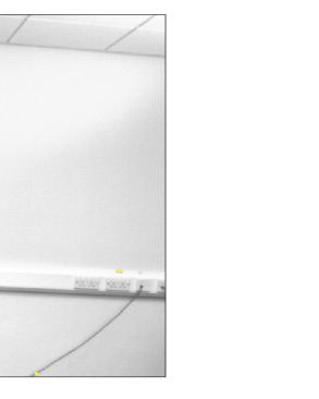
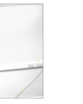
(b) Second image pair

(c) 3D point sets

(d) ECMPR-rigid

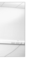
(e) ICP

Figure 5: Comparison between ECMPR-rigid and ICP applied to stereo data. (a) The first stereo image pair of a walking person. (b) The second stereo pair. The person performed a translational motion of 280 mm towards the camera and from right to left. (c) The two sets of 3D points before registration (223 model points and 249 data points). The result of matching with (d) ECMPR and with (e) ICP are shown superimposed onto the left image of the first pair. In this example, ECMPR found 95 inliers while ICP found 177 inliers. Both algorithms estimated the correct rotation. ICP failed to estimate the correct translation (see Table II for a quantitative comparison).

TABLE II: Comparison between ECMPR-rigid and ICP applied to the stereo data of Fig. 5.

Algorithm	Number of iterations	Number of inliers	Translation error (%)	Minimization error (mm)
ECMPR	12	95	12.5	4.6
ICP (Worst)	4	227	34.6	6.0
ICP (Best)	6	177	22.4	4.9

We also applied both ECMPR-rigid and ICP to real data obtained with a stereo camera pair as shown on Fig. 5 and Table II: The two stereo image pairs of a walking person were grabbed at two diffierent time instances. Two sets of 3D points were reconstructed from these two image pairs, Fig. 5-(c). The first set has 223 “model” points and the second set has 249 “data” points. These 3D points belong either to the walking person or to the static background. Fig. 5-(d) shows the matches found by ECMPR-rigid and Fig. 5-(e) shows the matches found by ICP. Table II summarizes the results. Both algorithms were initialized with $\mathbf{R}=\mathbf{I}$ and $\mbox{{\boldmath$t$}}=\mbox{{\boldmath$0$}}$. The error in translation is computed with $\|\mbox{{\boldmath$t$}}-\mbox{{\boldmath$t$}}_{g}\|/\|\mbox{{\boldmath$t$}}_{g}\|$ where $t$ is the estimated translation vector and $\mbox{{\boldmath$t$}}_{g}$ is the ground truth. The minimization error is computed with the square root of $1/n_{in}\sum_{i=1}^{n_{in}}\|\mbox{{\boldmath$Y$}}_{i}-\mathbf{R}\mbox{{\boldmath$X$}}_{i}-\mbox{{\boldmath$t$}}\|^{2}$ where $n_{in}$ is the number of inliers estimated by each algorithm. ICP was run with different threshold values. In all cases (ECMPR and ICP) the rotation matrix is correctly estimated.

VII-B Experiments with ECMPR-articulated

We tested ECMPR-articulated on a hand-tracking task, with both simulated and real data. We note that recent work in this topic uses specific constraints such as skin texture, skin shading[52] or skin color [53] that are incorporated into the hand model, together with a variational framework [52] or a probabilistic graphical [53] model that are tuned to the task of hand tracking. We did not attempt to devise such a special-purpose hand tracker from our general-purpose articulated registration algorithm.

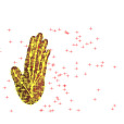
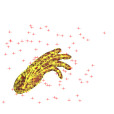
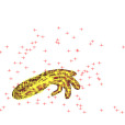
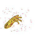
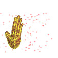
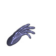
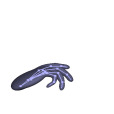
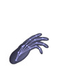
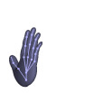
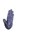
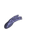
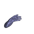
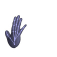
Figure 6: Top row: the ground-truth of the simulated poses and the simulated data (inliers and outliers). Milddle row: a correct registration result. Bottom row: ECMPR failed to correctly estimate all the kinematic parameters due to an improper initialization of the covariance matrix.

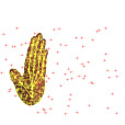
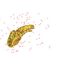
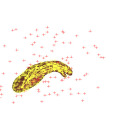
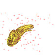
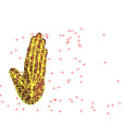
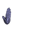
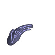
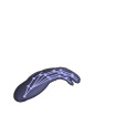
Figure 7: Another simulated sequence and the result of ECMPR.

The hand model used in all our experiments consists in five kinematic chains that share a common root part – the palm. Each kinematic chain is composed of four rigid parts, one part for the palm and three other parts for the phalanges composing each finger. Altogether, the kinematic hand model has 16 rigid parts and 21 rotational degrees of freedom (5 rotations for the thumb and 4 rotations for the other fingers). With the additional six degrees of freedom (three rotations and three translations) associated with the free motion of the palm, the hand has a total of 27 degrees of freedom. Each hand-part is modeled with an ellipsoid with fixed dimensions. Model points are obtained by uniformly sampling the surface of each one of these ellipsoids. This representation also allows to define an articulated implicit surface over the set of ellipsoids [35, 54, 55, 38]. Here we only use this implicit surface representation for visualization purposes.

(a) Ground-truth parameters

(b) Correct parameter estimation

(c) Incorrect parameter estimation

Figure 8: (a) Simulated trajectories of two angular joints associated with the first and second phalanges of the index finger. (b) Good estimation of these angle values. (c) Bad estimation of the angle values due to improper initialisation of the covariance matrix in ECMPR. These trajectories correspond to the examples shown in Fig. 6.

A commonly used strategy, in almost every articulated object tracking algorithm, is to specify joint-limit constraints thus preventing impossible kinematic poses. It is straightforward to impose such linear constraints into our convex optimization framework, i.e., section V-B. Indeed, inequality constraints can be incorporated into (34) without affecting the convexity nature of the problem. In practice we did not implement joint-limit constraints and hence the solutions found in the examples described below correspond exactly to (34).

In the case of simulated data, we animated the hand model just described in order to produce realistic articulated motions and to generate sets of model points, one set for each pose of the model. In practice, all the experiments described below used 15 model points for each hand part which corresponds to a total of 240 model points namely $\mbox{{\boldmath$X$}}_{i}^{(p)}$ with $1\leq i\leq 15$ and $0\leq p\leq 15$.

In order to simulate realistic observations we added Gaussian noise to the surface points. The standard deviation of the noise was 10% of the size of the bounding box of the data set. We also added outliers drawn from a uniform distribution defined over the volume occupied by the working space of the hand. In all these simulations the data sets contain 30% of outliers, i.e., there are 240 model points, 240 inliers and 72 outliers.

Fig. 6 and Fig. 7 show two experiments performed with simulated hand motions. Each one of these simulated data (top rows) contains a sequence of 120 articulated poses. We applied our registration method to these sequences, we estimated the kinematic parameters, and we compared them with the ground truth. ECMPR-articulated is applied in parallel to the five kinematic chains. First, ECMPR-rigid registers the root part (the hand palm) common to all the chains. Second, ECMPR-rigid is applied to the first phalanx of the index, middle, ring, and baby fingers. Third, it is applied to the second phalanx, etc.

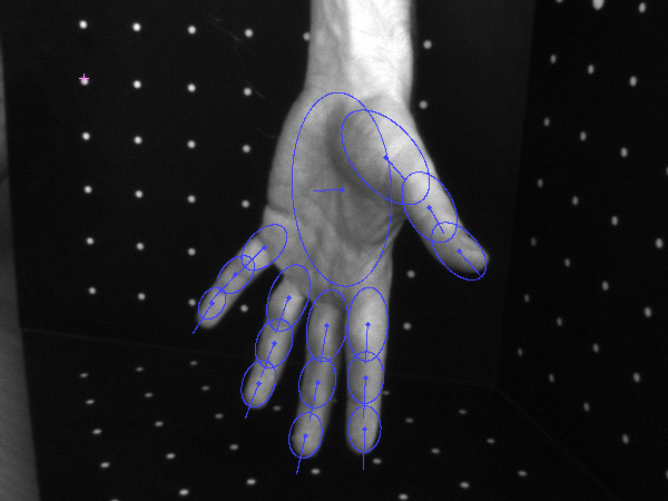
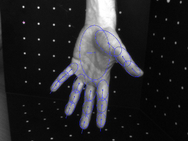
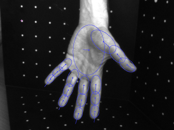
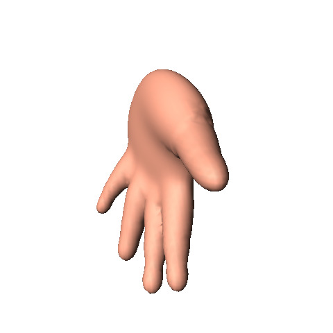
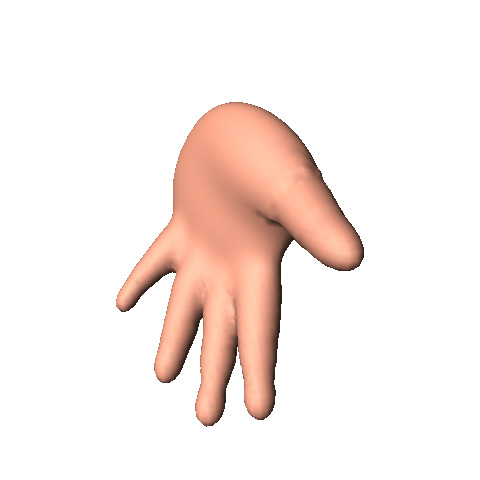
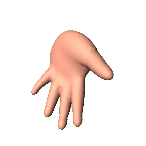
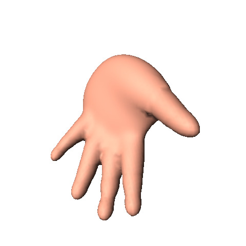
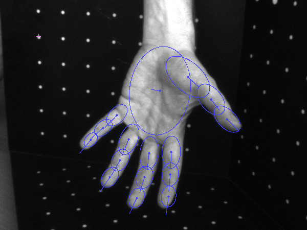
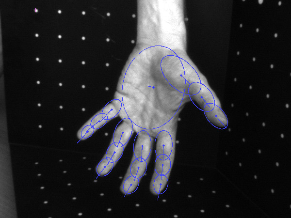
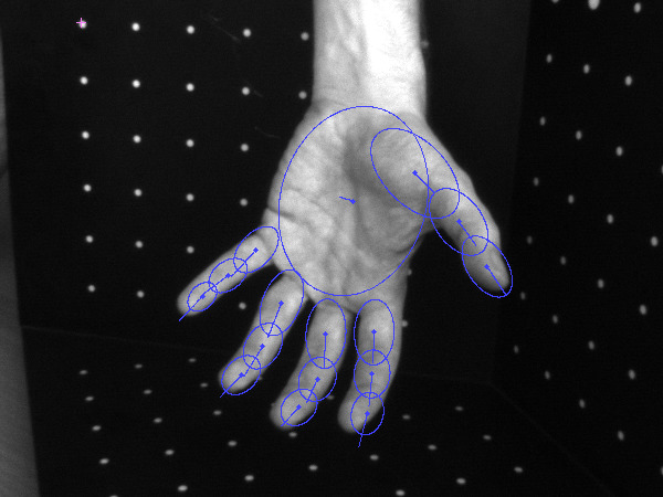
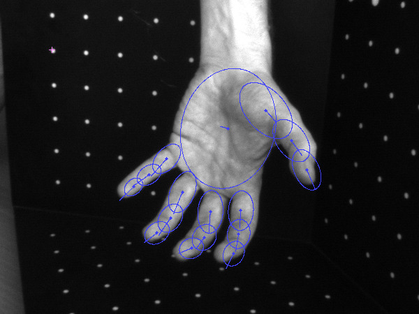
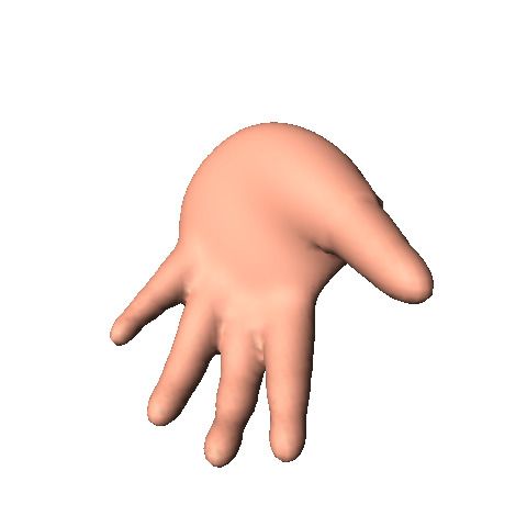
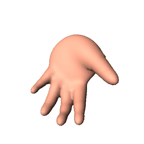
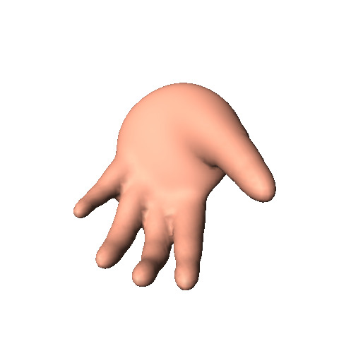
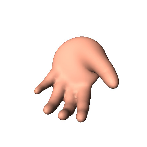
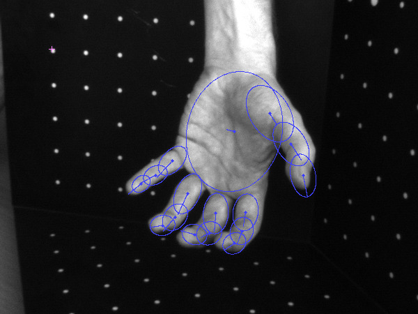
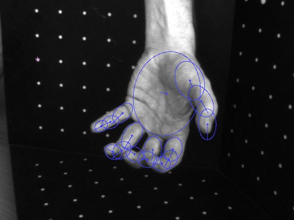
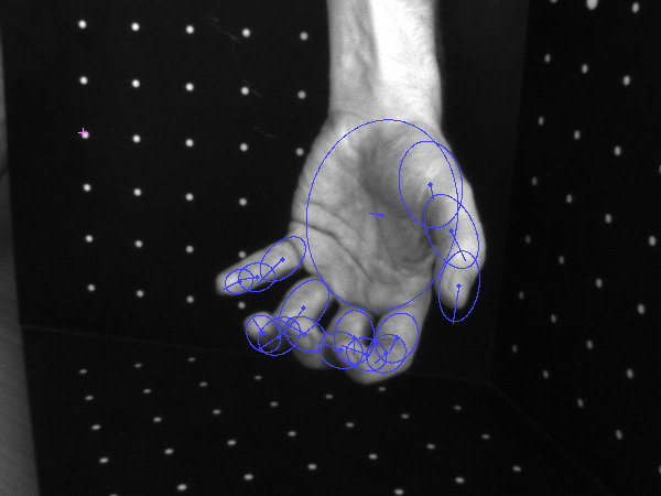
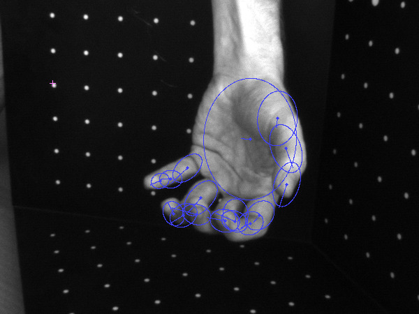
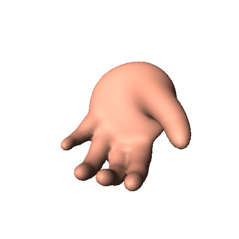
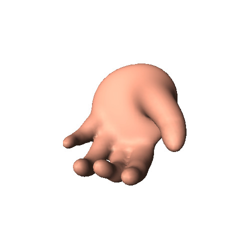
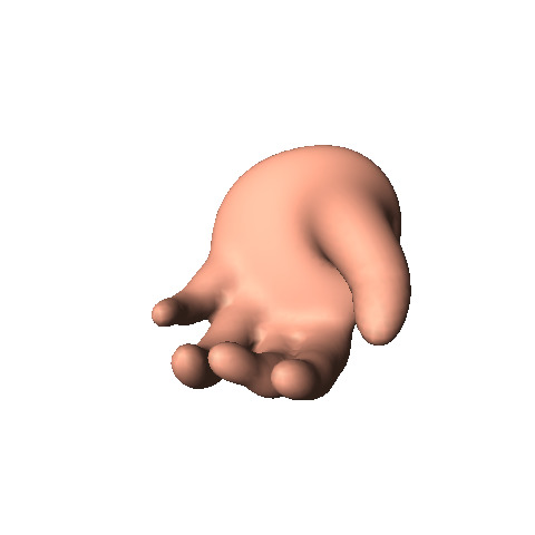
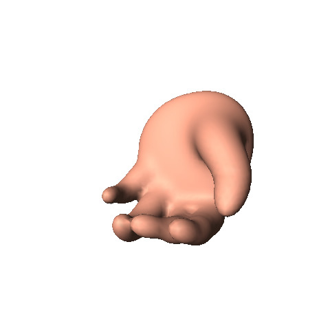
Figure 9: The image of a hand and the result of tracking for a grasping movement.

Fig. 6 shows a sequence of simulated poses (top row) and the results obtained with our algorithm (middle and bottom rows). When starting with a large covariance, ECMPR correctly estimated the articulated poses of the simulated hand (middle row). Starting with small covariances is equivalent to consider the data points that are in the neighbourhood of the model points and to disregard data points that are farther away from the current model point positions. In this case the trajectory of the thumb has been correctly estimated but the other four fingers failed to bend (bottom row). Notice, however, that in both cases the tracker has been able to “catch up” with these finger motions and to reduce the discrepancy between the estimated trajectories and the ground truth. The simulated trajectories and the estimated trajectories of the first and second phalanges of the index finger are shown on Fig. 8. Fig. 7 shows another experiment on a different simulated sequence.

These experiments yielded very good results. As expected, the percentage of outliers barely affected the registration results. These experiments confirmed the importance of using an anisotropic covariance model as well as the fact that covariance initialization is crucial. All the instances of the ECMPR-rigid algorithm (embedded in ECMPR-articulated) are initialized with large spherical covariances. While this increases the number of EM iterations, it allows the algorithm to escape from local minima.

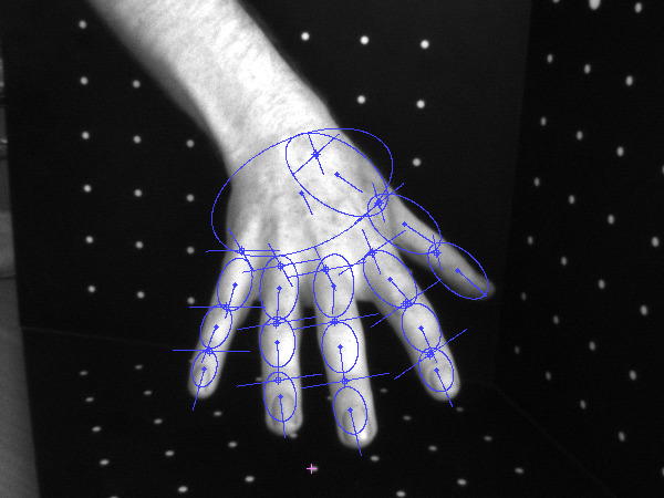
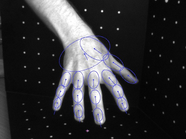
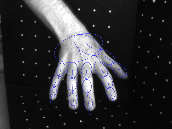
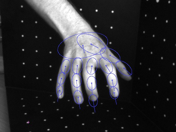
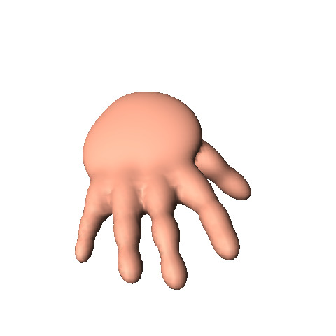
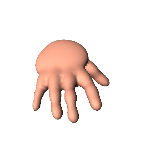
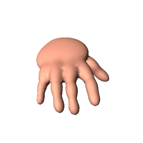
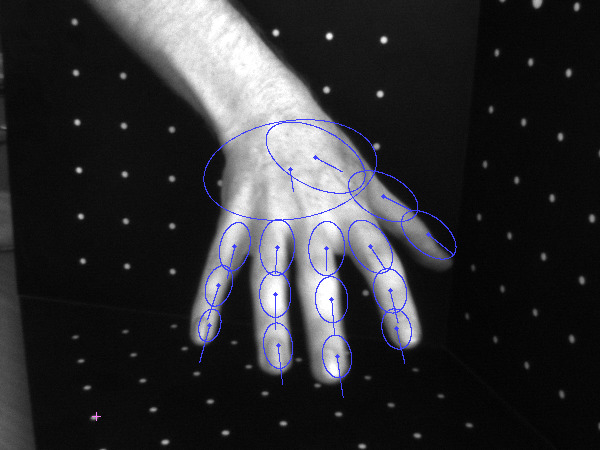
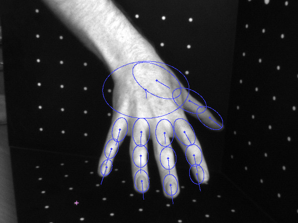
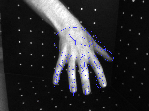
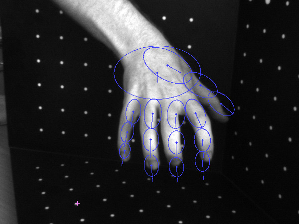
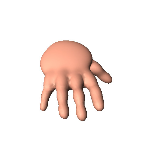
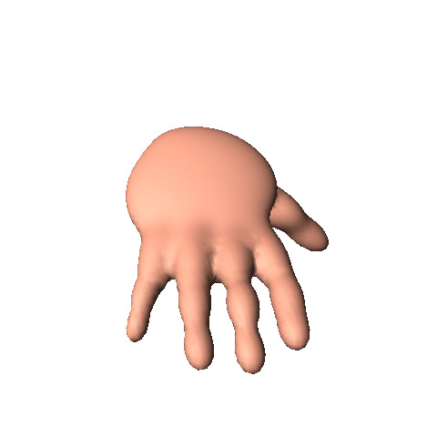
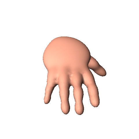
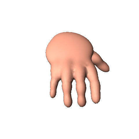
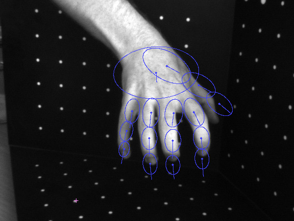
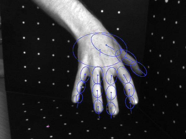
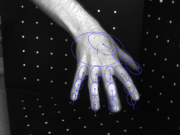
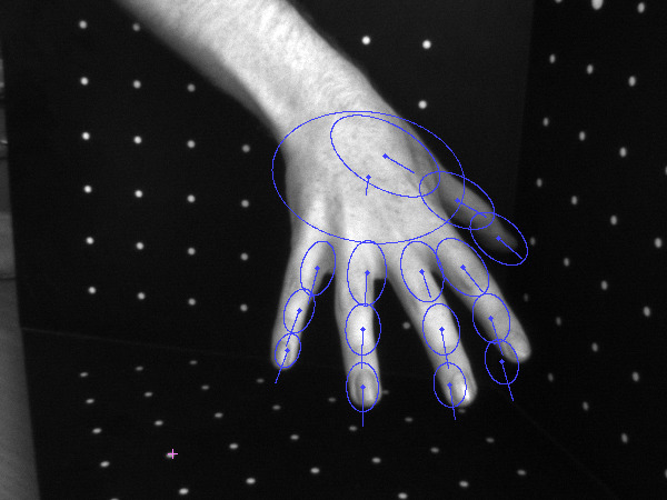
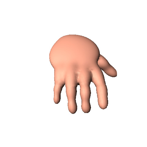
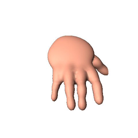
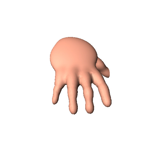
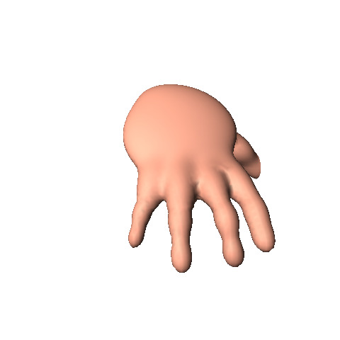
Figure 10: A similar grasping movement but the hand is viewed from above.

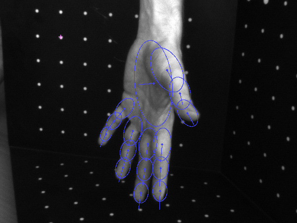
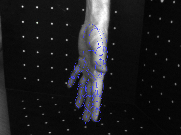
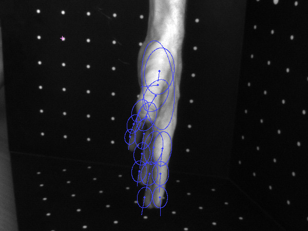
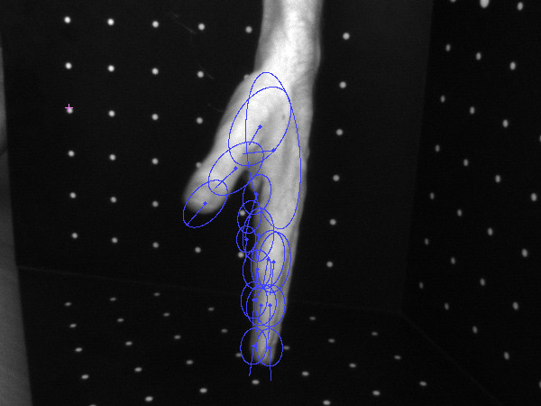
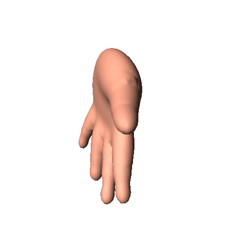
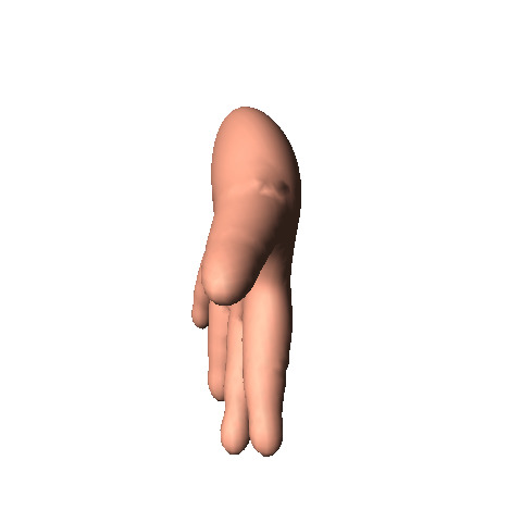
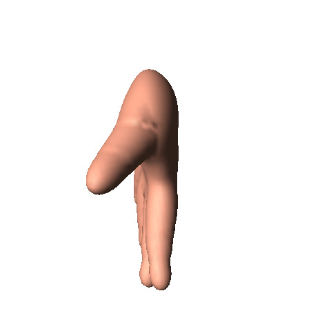
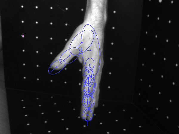
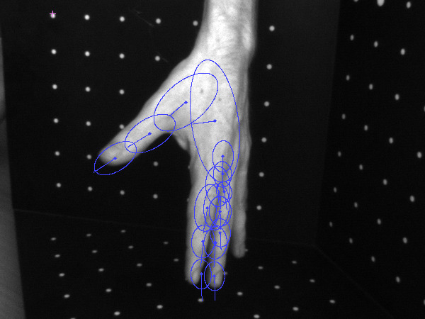
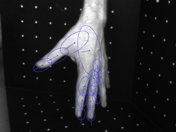
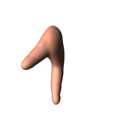
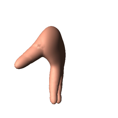
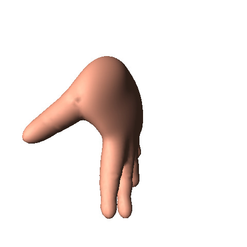
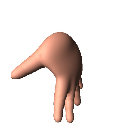
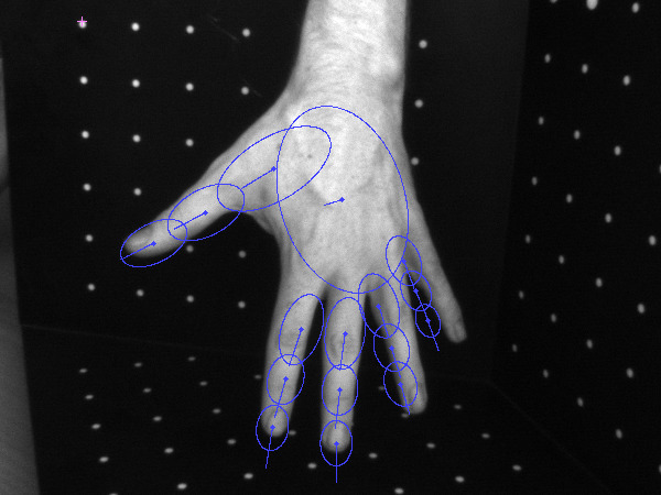
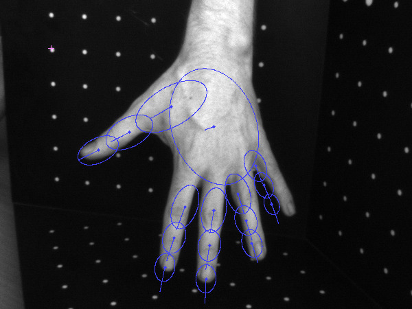
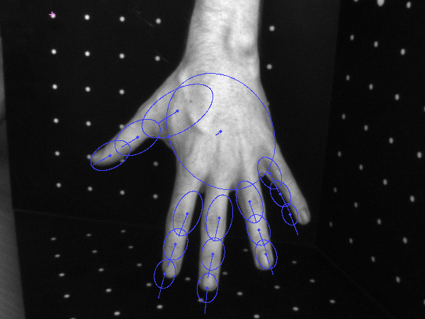
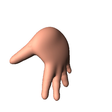
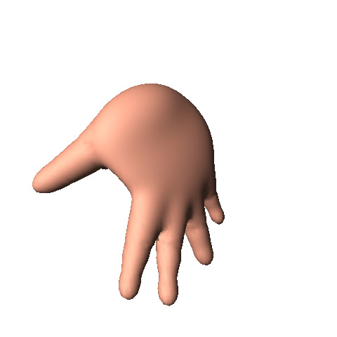
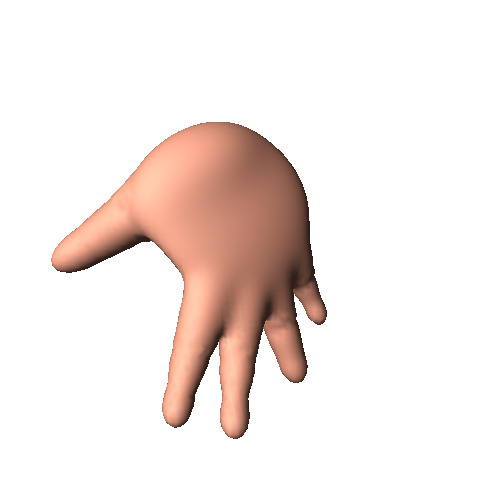
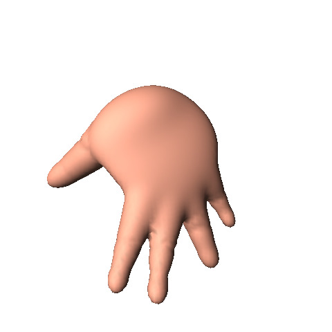
Figure 11: A rotational movement of the hand around an axis parallel to the image plane causes the fingers to disappear from the left-hand side of the image and appear again onto the right-hand side. These occlusions have as a result a very coarse initialization of the current pose. In spite of this problem the tracker performs quite well due to re-initialization of the covariance matrix at each time step of the tracker.

We then tested our method with real data consisting in several hand motions observed with a stereoscopic camera system, Fig 1. Each data sequence that we used contains 100 image pairs gathered at 20 frames per second. We run a standard stereo algorithm to estimate 3-D points. This yielded 500 to 1000 reconstructed points at each time step. The noise associated with these stereo data is inherently anisotropic because of the inaccuracy in depth. Moreover, there are many outliers that correspond either to data points which do not lie on the hand or to stereo mismatches.

The results of applying ECMPR to these data sets are illustrated on Figs. 9, 10 and 11. In the first and second examples the hand performs a grasping movement. In the third example the hand rotates around an axis roughly parallel to the image plane. In all these cases the algorithm selected, on average, 250 inliers per frame; This number roughly corresponds to the number of model points being considered (240). All the other data points were assigned to the outlier class. Notice that the number of data points vary a lot (500 to 1000 observations at each frame) and that the outlier rejection mechanism that we propose in this paper does not need to know in advance the percentage of outliers.

Note that along these motion sequences the hand flips from one side to another side while the positions and orientations of the fingers vary considerably. This means that it is often the case that almost all the model points that were currently registered, may suddenly disappear while other model points suddenly appear. This is one of the main difficulties associated with registering articulated objects. Therefore, during the tracking, the algorithm must perform some form of bootstrapping, i.e., it must establish data-point-to-model-point assignments from scratch. Re-initialization of the covariance matrix at each time step, along the lines described above, is crucial to the success of the registration/tracking algorithm.

VIII Conclusions

In this paper we addressed the problem of matching rigid and articulated shapes through robust point registration. The proposed approach has its roots in model-based clustering [22]. More specifically, the point registration problem is cast into the framework of maximum likelihood with hidden variables [21, 43, 44]. We formally derived a variant of the EM algorithm which maximizes the expected complete-data log-likelihood. This guarantees maximization of the observed-data log-likelihood. We showed that it is convenient to replace the standard M-step by three conditional maximization steps, or CM-steps, while preserving the convergence properties of EM.

Our approach differs significantly from existing methods for point registration, namely ICP and its variants [1, 2, 3, 4, 5, 6, 7, 8], soft assignment methods [9, 10, 11], as well as various EM implementations [13, 14, 15, 16, 17, 18]: The ECMPR-rigid and -articulated algorithms that we proposed fit a set of model points to a set of data points where each model point is the center of a Gaussian component in a mixture model. Each component in the mixture may have its own anisotropic covariance. Our method treats the data points and the model points in a non-symmetric way, which has several advantages: It allows to deal with a varying number of observations, either larger or smaller than the number of model points, it performs robust parameter estimation in the presence of data corrupted with noise and outliers, and it is based on a principled probabilistic approach.

More specifically, the method guarantees robustness via a uniform component added to the Gaussian mixture model. This built-in outlier rejection mechanism differs from existing outliers detection/rejection strategies used in conjunction with point registration, such as methods based on non-linear loss functions that can be trapped in local minima, or methods based on random sampling which are time-consuming and that can only deal with a limited number of outlying data.

In particular we put emphasis on a general model that uses anistropic covariance matrices, in which case the rotation associated with rigid alignment cannot be found in closed-form. This led us to approximate the associated non-convex optimization problem with a convex one. Namely, we showed how to transform the non-linear problem into a constrained quadratic optimization one and how to use semi-definite positive relaxation to solve it in practice.

We provided in detail the ECMPR-rigid algorithm. We showed how this algorithm can be incrementally applied to articulated registration using a novel kinematic representation that is well suited in the case of point registration.

In general, ECMPR performs better than ICP. In particular it is less sensitive to initialization and it is more robust to outliers. In the future we plan to investigate various ways of implementing our algorithm more efficiently. Promising approaches are based on modifying the standard E-step. A fast but suboptimal “winner take all” variant is Classification EM, or CEM, which consists in forcing the posterior probabilities to either 0 or 1 after each E-step [56]. We plan to study CEM in the particular context of point registration and, possibly, derive a more efficient implementation of ECMPR. This may also lead to a probabilistic interpretation of ICP, and hence to a better understanding of the links existing between probabilistic and deterministic registration methods. Other efficient variants of the E-step are based on structuring the data using either block-like organizations [57], or KD-trees [58]. We also plan to implement KD-trees in order to increase the efficiency of ECMPR.

[Expansion of $\mathbf{A}$ and $b$ in eq. (32)]

By expanding (28), substituting the optimal translation with (27) and rearranging terms, one obtains the following expressions for the 9$\times$9 matrix $\mathbf{A}$ and the 9$\times$1 vector $b$:

$$\mathbf{A}=\mathbf{N}-\mathbf{M}^{\top}\mathbf{K}\mathbf{M}$$ (45)

$$\mbox{{\boldmath$b$}}=\mathbf{M}^{\top}\mbox{{\boldmath$p$}}-\mbox{{\boldmath$q$}}$$ (46)

with:

$$\mathbf{N}_{9\times 9} = \sum_{i=1}^{n}\lambda_{i}\mbox{{\boldmath$X$}}_{i}\mbox{{\boldmath$X$}}_{i}^{\top}\otimes\mathbf{\Sigma}_{i}^{-1}$$

$$\mathbf{M}_{3\times 9} = \sum_{i=1}^{n}\lambda_{i}\mbox{{\boldmath$X$}}_{i}^{\top}\otimes\mathbf{\Sigma}_{i}^{-1}$$

$$\mathbf{K}_{3\times 3} = \left(\sum_{i=1}^{n}\lambda_{i}\mathbf{\Sigma}_{i}^{-1}\right)^{-1}$$

$$\mbox{{\boldmath$p$}}_{3\times 1} = \mathbf{K}\left(\sum_{i=1}^{n}\lambda_{i}\mathbf{\Sigma}_{i}^{-1}\mbox{{\boldmath$W$}}_{i}\right)$$

$$\mbox{{\boldmath$q$}}_{9\times 1} = \text{vec}\left(\sum_{i=1}^{n}\lambda_{i}\mathbf{\Sigma}_{i}^{-1}\mbox{{\boldmath$W$}}_{i}\mbox{{\boldmath$X$}}_{i}^{\top}\right)$$

The Kronecker product between the $m\times n$ matrix/vector $\mathbf{A}$ and the $p\times q$ matrix/vector $\mathbf{B}$ is the $mp\times nq$ matrix/vector defined by:

$$\mathbf{A}\otimes\mathbf{B}=\left[\begin{array}[]{ccc}A_{11}\mathbf{B}&\ldots&A_{1n}\mathbf{B}\\ \vdots&&\vdots\\ A_{m1}\mathbf{B}&\ldots&A_{mn}\mathbf{B}\end{array}\right]$$

Moreover, $\text{vec}(\mathbf{A})$ returns the $mn\times 1$ vector:

$$\text{vec}(\mathbf{A})=(A_{11}\ldots A_{mn})^{\top}$$

Radu Horaud received the B.Sc. degree in electrical engineering, the M.Sc. degree in control engineering, and the Ph.D. degree in computer science from the Institut National Polytechnique de Grenoble, Grenoble, France. He holds a position of Director of Research with the Institut National de Recherche en Informatique et Automatique (INRIA), Grenoble Rhône-Alpes, Montbonnot, France, where he is the head of the PERCEPTION team since 2006. His research interests include computer vision, machine learning, multisensory fusion, and robotics. He is an Area Editor of the Elsevier Computer Vision and Image Understanding, a member of the advisory board of the Sage International Journal of Robotics Research, and a member of the editorial board of the Kluwer International Journal of Computer Vision. He was a Program Cochair of the Eighth IEEE International Conference on Computer Vision (ICCV 2001).

Florence Forbes was born in Monaco in 1970. She received both the B.Sc. and M.Sc. degrees in computer science and applied mathematics from the Ecole Nationale Supérieure d’Informatique et Mathématiques Appliquées de Grenoble, Grenoble, France, and the Ph.D. degree in applied probabilities from University Joseph Fourier, Grenoble, France. Since 1998 she has been a research scientist with the Institut National de Recherche en Informatique et Automatique (INRIA), Grenoble Rhône-Alpes, Montbonnot, France, where she is the head of the MISTIS team since 2003. Her research activities include Bayesian image analysis, Markov models and hidden structure models.

Manuel Yguel received both the B.Sc. and M.Sc. degrees in computer science and applied mathematics from the Ecole Nationale Supérieure d’Informatique et Mathématiques Appliquées de Grenoble, Grenoble, France, and the Ph.D. degree in computer science from the Institut National Polytechnique de Grenoble, Grenoble, France. His research interests include autonomous robot navigation, multisensory fusion, and probabilistic SLAM.

Guillaume Dewaele received both the B.Sc. and M.Sc. degrees in Physics from Ecole Normale Supérieure, Lyon, France, and the Ph.D. degree in computer science from the Institut National Polytechnique de Grenoble, Grenoble, France. His research interests include modeling of deformable and articulated objects for computer animation and computer vision.

Jian Zhang is a Ph.D. student in the Department of Electrical and Electronic Engineering at the University of Hong Kong, Pokfulam, Hong Kong. In 2009 she spent 4 months at INRIA Grenoble Rhône-Alpes, Montbonnot, France, in the PERCEPTION team. Her research interestes include feature matching, motion tracking, and 3D reconstruction.

References

- [1] P. J. Besl and N. D. McKay, “A method for registration of 3-D shapes,” IEEE Transactions on Pattern Analysis and Machine Intelligence, vol. 14, pp. 239–256, February 1992.
- [2] Z. Zhang, “Iterative point matching for registration of free-form curves and surfaces,” International Journal of Computer Vision, vol. 13, pp. 119–152, 1994.
- [3] S. Rusinkiewicz and M. Levoy, “Efficient variants of the ICP algorithm,” in IEEE Proc. 3rd International Conference on 3D Digital Imaging and Modeling, Quebec, Canada, May-June 2001.
- [4] A. W. Fitzgibbon, “Robust registration of 2D and 3D point sets,” Image and Vision Computing, vol. 21, no. 12, pp. 1145–1153, December 2001.
- [5] D. Chetverikov, D. Stepanov, and P. Krsek, “Robust Euclidean alignment of 3D point sets: the trimmed iterative closest point algorithm,” Image and Vision Computing, vol. 23, no. 3, pp. 299–309, March 2005.
- [6] G. C. Sharp, S. W. Lee, and D. K. Wehe, “Maximum-likelihood registration of range images with missing data,” IEEE Transactions on Pattern Analysis and Machine Intelligence, vol. 30, no. 1, pp. 120–130, January 2008.
- [7] D. Demirdjian, “Combining geometric- and view-based approaches for articulated pose estimation,” in European Conference on Computer Vision, vol. III, 2004, pp. 183–194.
- [8] L. Munderman, S. Corazza, and T. P. Andriacchi, “Accurately measuring human movement using articulated ICP with soft-joint constraints and a repository of articulated models,” in IEEE Proc. of the Eleventh International Conference on Computer Vision, Rio de Janeiro, Brazil, November 2007.
- [9] A. Rangarajan, H. Chui, and F. L. Bookstein, “The softassign procrustes matching algorithm,” in Information Processing in Medical Imaging (IPMI), 1997, pp. 29–42.
- [10] H. Chui and A. Rangarajan, “A new point matching algorithm for non-rigid registration,” Computer Vision and Image Understanding, vol. 89, no. 2-3, pp. 114–141, February 2003.
- [11] Y. Liu, “Automatic 3D free form shape matching using the graduated assignment algorithm,” Pattern Recognition, vol. 38, pp. 1615–1631, 2005.
- [12] ——, “A mean field annealing approach to accurate free form shape matching,” Pattern Recognition, vol. 40, pp. 2418–2436, 2007.
- [13] W. Wells III, “Statistical approaches to feature-based object recognition,” International Journal of Computer Vision, vol. 28, no. 1/2, pp. 63–98, 1997.
- [14] H. Chui and A. Rangarajan, “A feature registration framework using mixture models,” in Proc. of IEEE Workshop on Mathematical Methods in Biomedical Image Analysis, 2000, pp. 190–197.
- [15] S. Granger and X. Pennec, “Multi-scale EM-ICP: A fast and robust approach for surface registration,” in European Conference on Computer Vision, vol. IV, 2002, pp. 418–432.
- [16] A. Myronenko, X. Song, and M. A. Carreira-Perpinan, “Non-rigid point set registration: Coherent point drift,” in Proc. of Advances in Neural Information Processing Systems, December 2006, pp. 1009–1016.
- [17] M. Sofka, G. Yang, and C. V. Stewart, “Simultaneous covariance driven correspondence (CDC) and transformation estimation in the expectation maximization framework,” in Proceedings of the IEEE Conference on Computer Vision and Pattern Recognition, June 2007.
- [18] B. Jian and B. C. Vemuri, “A robust algorithm for point set registration using mixture of Gaussians,” in IEEE Proc. of the Tenth International Conference on Computer Vision, Beijing, Chian, 2005.
- [19] P. Meer, “Robust techniques for computer vision,” in Emerging Topics in Computer Vision. Prentice Hall, 2004.
- [20] R. Sinkhorn, “A relationship between arbitrary positive matrices and doubly stochastic matrices,” Annals of Mathematical Statistics, vol. 35, pp. 876–879, 1964.
- [21] A. P. Dempster, N. M. Laird, and D. B. Rubin, “Maximum likelihood estimation from incomplete data via the EM algorithm (with discussion),” Journal of the Royal Statistical Society, Series B, vol. 39, pp. 1–38, 1977.
- [22] C. Fraley and A. E. Raftery, “Model-based clustering, discriminant analysis, and density estimation,” Journal of the American Statistical Association, vol. 97, pp. 611–631, 2002.
- [23] K. S. Arun, T. S. Huang, and S. D. Blostein, “Least-squares fitting of two 3-D point sets,” IEEE Trans. on Pattern Analysis and Machine Intelligence, vol. 9, no. 5, pp. 698–700, September 1987.
- [24] B. Horn, “Closed-form solution of absolute orientation using orhtonormal matrices,” J. Opt. Soc. Amer. A., vol. 5, no. 7, pp. 1127–1135, 1987.
- [25] ——, “Closed-form solution of absolute orientation using unit quaternions,” J. Opt. Soc. Amer. A., vol. 4, no. 4, pp. 629–642, 1987.
- [26] S. Umeyama, “Least-squares estimation of transformation parameters between two point patterns,” IEEE Transactions on Pattern Analysis and Machine Intelligence, vol. 13, no. 4, pp. 376–380, April 1991.
- [27] J. Williams and M. Bennamoun, “A multiple view 3D registration algorithm with statistical error modeling,” IEICE Transactions on Information and Systems, vol. E83-D, no. 8, pp. 1662–1670, August 2000.
- [28] A. I. Yuille, P. Stolorz, and J. Utans, “Statistical physics, mixture of distributions, and the EM algorithm,” Neural Computation, vol. 6, pp. 334–340, 1994.
- [29] B. Luo and E. Hancock, “A unified framework for alignment and correspondence,” Computer Vision and Image Understanding, vol. 92, no. 1, pp. 26–55, October 2003.
- [30] Y. Tsin and T. Kanade, “A correlation-based approach to robust point set registration,” in Proceedings of the Eighth European Conference on Computer Vision, Prague, Czeh Republic, May 2004.
- [31] F. Wang, B. Vemuri, A. Rangarajan, I. Schmalfuss, and S. Eisenschenk, “Simultaneous nonrigid registration of multiple point sets and atlas construction,” in Proceedings of the Ninth European Conference on Computer Vision, Graz, Austria, May 2006.
- [32] X.-L. Meng and D. B. Rubin, “Maximum likelihood estimation via the ECM algorithm: a general framework,” Biometrika, vol. 80, pp. 267–278, 1993.
- [33] C. Lemarechal and F. Oustry, “SDP relaxations in combinatorial optimization from a Lagrangian viewpoint,” in Advances in Convex Analysis and Global Optimization, Hadjisavvas and Panos, Eds. Kluwer Academic Publishers, 2001, ch. 6, pp. 119–134.
- [34] I. Kakadiaris and D. Metaxas, “Model-based estimation of 3d human motion,” IEEE Transactions on Pattern Analysis and Machine Intelligence, vol. 22, no. 12, pp. 1453–1459, 2000.
- [35] R. Plaenkers and P. Fua, “Articulated soft objects for multi-view shape and motion capture,” IEEE Transactions on Pattern Analysis and Machine Intelligence, vol. 25, no. 9, pp. 1182–1187, 2003.
- [36] C. Bregler, J. Malik, and K. Pullen, “Twist based acquisition and tracking of animal and human kinematics,” International Journal of Computer Vision, vol. 56, no. 3, pp. 179–194, February - March 2004.
- [37] D. Knossow, R. Ronfard, and R. Horaud, “Human motion tracking with a kinematic parameterization of extremal contours,” International Journal of Computer Vision, vol. 79, no. 2, pp. 247–269, September 2008.
- [38] R. Horaud, M. Niskanen, G. Dewaele, and E. Boyer, “Human motion tracking by registering an articulated surface to 3-D points and normals,” IEEE Transactions on Pattern Analysis and Machine Intelligence, vol. 31, no. 1, pp. 158–164, January 2009.
- [39] S. Pellegrini, K. Schindler, and D. Nardi, “A generalization of the ICP algorithm for articulated bodies,” in Proc. of the British Machine Vision Conference, September 2008.
- [40] J. D. Banfield and A. E. Raftery, “Model-based Gaussian and non-Gaussian clustering,” Biometrics, vol. 49, no. 3, pp. 803–821, September 2002.
- [41] C. Hennig, “Breakdown points for maximum likelihood estimators of location-scale mixtures,” The Annals of Statistics, vol. 32, no. 4, pp. 1313–1340, 2004.
- [42] C. Hennig and P. Coretto, “The noise component in model-based cluster analysis,” in Proceedings of the 31st Annual Conference of the German Classification Society on Data Analysis, Machine Learning, and Applications, Freiburg, Germany, March 2007.
- [43] R. A. Redner and H. F. Walker, “Mixture densities, maximum likelihood and the EM algorithm,” SIAM Review, vol. 26, no. 2, pp. 195–239, April 1984.
- [44] G. J. McLachlan and T. Krishnan, The EM Algorithm and Extensions. New-York: Wiley, 1997.
- [45] P. J. Rousseeuw, “Least median of squares regression,” Journal of the American Statistical Association, vol. 79, pp. 871–880, 1984.
- [46] P. J. Rousseeuw and S. Van Aelst, “Positive-breakdown robust methods in computer vision,” in Computing Science and Statistics, Berk and Pourahmadi, Eds. Interface Foundation of North America, 1999, vol. 31, pp. 451–460.
- [47] C. Bishop, Pattern Recognition and Machine Learning. Springer, 2006.
- [48] S. Ingrassia and R. Rocci, “Constrained monotone EM algorithms for finite mixture of multivariate Gaussians,” Computational Statistics and Data Analysis, vol. 51, pp. 5339–5351, 2007.
- [49] R. J. Hathaway, “A constrained formulation of maximum-likelihood estimation for normal mixture distributions,” Annals of Statistics, vol. 13, pp. 795–?800, 1985.
- [50] C. Lemarechal and F. Oustry, “Semidefinite relaxations and Lagrangian duality with application to combinatorial optimization,” INRIA, Tech. Rep. 3710, June 1999.
- [51] J. M. McCarthy, Introduction to Theoretical Kinematics. Cambridge: MIT Press, 1990.
- [52] M. de la Gorce, N. Paragios, and D. Fleet., “Model-based hand tracking with texture, shading and self-occlusions,” in Proc. of Computer Vision and Pattern Recognition, June 2008.
- [53] H. Hamer, K. Schindler, E. Koller-Meier, and L. Van Gool, “Tracking a hand manipulating an object,” in Proc. of International Conference on Computer Vision, October 2009.
- [54] G. Dewaele, F. Devernay, and R. Horaud, “Hand motion from 3D point trajectories and a smooth surface model,” in Proc. of the Eighth European Conference on Computer Vision, ser. LNCS 3021, vol. I. Springer, May 2004, pp. 495–507.
- [55] G. Dewaele, F. Devernay, R. Horaud, and F. Forbes, “The alignment between 3-D data and articulated shapes with bending surfaces,” in Proc. of the Ninth European Conference on Computer Vision, ser. LNCS 3953, vol. III. Springer, May 2006, pp. 578–591.
- [56] G. Celeux and G. Govaert, “A classification EM algorithm for clustering and two stochastic versions,” Computational statistics and data analysis, vol. 14, no. 3, pp. 315–332, 1992.
- [57] B. Thiesson, C. Meek, and D. Heckerman, “Accelerating EM for large databases,” Machine Learning, vol. 45, no. 3, pp. 279–299, 2001.
- [58] J. Verbeek, J. Nunnink, and N. Vlassis, “Accelerated em-based clustering of large data sets,” Data Mining and Knowledge Discovery, vol. 13, no. 3, pp. 291–307, November 2006.