Einstein-Æther Gravity in the light of Event Horizon Telescope Observations of M87*

Abstract

We investigate Einstein-Æther gravity in light of the recent Event Horizon Telescope (EHT) observations of the M87*. The shape and size of the observed black hole shadow contains information of the geometry in its vicinity, and thus one can consider it as a potential probe to investigate different gravitational theories, since the involved calculation framework is enriched with different size-rotation features as well as with extra model parameters. In the case of Einstein-Æther gravity the black hole solutions include two classes depending on the involved æther parameters. We calculate the corresponding photon effective potential, the unstable photon sphere radius, and finally the induced angular size, which combined with the mass and the distance can lead to a single prediction that quantifies the black hole shadow, namely the diameter per unit mass $d$. Since $d_{M87*}$ is observationally known from the EHT Probe, we extract the corresponding parameter regions in order to obtain consistency. We find that Einstein-Æther black hole solutions agree with the shadow size of EHT M87*, if the involved Æther parameters are restricted within specific ranges, along with an upper bound on the dimensionless spin parameter $a$, which is verified by a full scan of the parameter space within $1\sigma$-error.

1 Introduction

In recent years, due to considerable developments in observational astronomy, accessible doors such as X-ray binaries, gravitational waves, and black-hole shadow have been opened onto the study of black holes (BHs), leading to the possibility to investigate the nature and traits of gravity in the strong-field regime. The first are actually X-rays emitted from a binary system due to matter falling from one normal star into its companion, which usually is a collapsed star, such as a neutron star or a BH [1]. On the other hand, gravitational waves observations arise from a series of binary BH and neutron star mergers recorded by LIGO-Virgo Consortium [2]-[8]. It is expected that in the not too distant future, by improving the signal-to-noise due to the increased number of merging events, such observations will be able to reveal more deep aspects of BH physics.

The black-hole shadow has become one of the most exciting events in observational astronomy, in the light of recording the first stunning new radio images of the supermassive BH that resides at the center of nearby galaxy M87* by “Event Horizon Telescope” (EHT) (which incorporates the technology called “mm-band Very Long Baseline Interferometry” (VLBI) and images the emissions close to supermassive BHs) [9]-[14] at April 2019. In particular, it provided the first visual evidence indicating directly the existence of a compact object such as a supermassive BH. Note that the defining feature that distinguished a BH from other objects such as a wormhole or a naked singularity is the event horizon, the boundary from within which nothing can escape. Due to the controversy about the distinction between a BH shadow and a wormhole [15, 16] or naked singularity [17, 18, 19, 20, 21] ones, as well as due to the lack of recording thermal radiation indicating the direct existence of event horizon [22, 23], it is reasonable to adopt a conservative approach and consider that the shadow image released by the EHT collaboration actually reveals an image near to the event horizon, at least as close as the light ring orbits [24].

Historically the concept of the black hole shadow comes from the 70’s with the seminal works [26, 27] and [28], which respectively had been performed for the cases of Schwarzschild BH and rotating Kerr BH. In the light of these studies it was found that the non-rotating BH has a perfect circular shadow [29], while by taking the rotation into account the shape of shadow is elongated due to the dragging effect. Nevertheless, the idea to image the shadow of BH by taking advantage of VLBI technology, appeared in [30].

The dark area over a brighter background in the center of the image is termed the “BH’s shadow”, and it is predicted by general relativity as the null geodesics in the strong gravity area [24, 25]. Generally speaking, photons follow several paths depending on their angular momentum: large, small, and critical. The first sets of photons coming from infinity will be bounded back to infinity by the gravitational potential of the BH. The second sets of photons will fall into the BH, which results in a dark area for the distant observer. However, the third sets, namely the photons with critical angular momentum, will swirl around the BH one ring by one ring which makes the unstable boundary of the shadow. This is the same as the shining halo observed in EHT image, which is expected to be comprised of photons from the hot, radiating gas that surrounds the BH, whose paths have been bent around the BH before arriving at the telescopes. Although close to the BH shadow the strong gravitational lensing may be quite obvious, however, it is expected that the shadows are far more easily to be observed, since unlike one-dimensional lensing images the BH shadows are two-dimensional dark regions.

Extracting the information saved in the shadow image released by EHT, which due to the new imaging techniques enjoys ultra-high angular resolution, conducts us to understand in a more transparent way significant issues such as the matter accretion process and BH jets. It also able to shed light on various metric theories of gravity [31, 32, 33]. Hence, after the EHT announcement, a large amount of research has been devoted in calculating the shadows of a vast class of BH solutions [34]-[59] and the confrontation with the extracted information from EHT BH shadow image of M87* [60]-[69], investigating fundamental physics issues too [70]-[85]. Additionally, one can also examine the BH shadow in the interplay with other related concepts, such as quasinormal modes, deflection of light, quasiperiodic oscillations, etc [86]-[93]. Moreover, some BH shadow studies, in the light of employing general relativistic (GR) magnetohydrodynamic simulations of magnetized accretion flows onto BH, are able to provide a more solid knowledge, see e.g [32, 94, 95, 96, 97, 98].

Nevertheless, given that the shape and size of the shadow contains traces of the geometry vicinity of the BH, and similarly to the quasinormal modes approach, one can consider the shadow as a potential probe to investigate the BH structure within different gravitational theories. In particular, although general relativity is a well-behaved theory at low energy, infrared (IR), scales and has come out proudly from numerous tests, when high energy, ultra-violet (UV) effects are involved one might need gravitational extensions or modifications, namely theories that possess general relativity as a low-energy limit but in general having a richer structure. Hence, one expects advantages such as improvements of the singularity behavior, of renormalizability, or of cosmological phenomenology.

One of the fundamental principles of general relativity that might be altered in the UV limit due to the quantization of gravity is the Lorentz’s invariance (LI), since Lorentz symmetry is not fundamental in the sense that it depends on the scale we are exploring nature’s energy [99, 100, 101]. Breaking Lorentz symmetry in the UV may imply the existence of a preferred frame at Planck scale. Small departures from LI could be used in order to study physics at the fundamental level, via investigation of Standard Model Extensions as an effective field theory framework [102] (see also [103]). By extending the LI breaking into gravity sector, a number of well known modified theories arise, such as Einstein-Æther [104, 105, 106, 107, 108, 109, 110], Horava-Lifshitz [111, 112, 113], mimetic gravity [114, 115], Finsler gravity [116, 117] etc. Although the LI breaking in the above theories arise from different mechanisms, one can explore the general features in a unified way [118].

The Einstein-Æther (EA) theory is a generally covariant theory of gravity, which violates the LI locally by possessing a dynamical, unit-norm and timelike vector field, called “æther field”, which defines a preferred timelike direction at each spacetime point. EA gravity includes a number of coupling constants called æther parameters, which are tightly constrained by gravitational wave events such as GW170817 and GRB170817A [7, 8, 119]. Similarly to most modified theories of gravity, one can investigate BH solutions in EA theory, considering an asymptotically flat spacetime. In particular, using two specific mixing of the æther parameters, one derives two sets of static and spherically symmetric BH solutions [120, 121], while extension to charged solutions has been obtained in [122] (see also [123] for a systematic study of the spherically symmetric static spacetimes in this framework).

In the present work we are interested in investigating EA theory using the EHT observations of the M87*. In particular, since the EA-gravity BH solutions incorporate the effects of the æther field, this field will affect the corresponding shadow too, and hence confrontation with EHT observations will reveal if the theory at hand is in agreement with them or if it must be constrained or excluded completely. The crucial ingredient of the analysis is that although the EHT’s collaboration focuses on the Kerr BH solution in the background of general relativity [13, 124, 85], namely incorporating the angular size and rotation in a specific and relative restricted framework, allowing for a modified gravity as the underlying theory enriches the calculation framework with different size-rotation features as well as with extra model parameters. And this procedure will be more efficient in theories which possess various corrections on the Kerr-metric solutions, such is the case in Einstein-Æther gravity. Besides, since the validity of the assumptions used in the measurement (for instance on rotation) cannot be deduced solely from the correspondence between theory and data, one can have theories beyond general relativity that incorporate successfully the data too [85].

The manuscript is structured as follows: In Section 2 we briefly review the slowly rotating BH solutions in the EA gravity. In Section 3 we determine the null geodesics equations as well as the orbital equations of photons, and we investigate the shadows related to two types of slowly rotating AE BH solutions. In Section 4 we confront the obtained shadows with the EHT image of supermassive object in M87*, and we extract explicit constraints on the coupling parameters of the EA theory. We eventually summarize our results and conclude in Section 5. Throughout the manuscript we adopt natural units where $\hbar=k_{B}=c=1$.

2 Rotating black-hole solutions in Einstein-Æther gravity

In this Section we present the extraction of slowly rotating black-hole solutions in the framework of Einstein-Æther (AE) gravity. The action of the EA theory is [104, 106]

$$S=S_{EH}+S_{AE}=\frac{1}{16\pi G_{AE}}\int d^{4}x\sqrt{-g}\Big{(}R+\mathcal{L}_{AE}\Big{)},$$ (2.1)

which includes the standard Einstein-Hilbert action $S_{EH}$ plus the æther action $S_{AE}$. In the above action, $R$, $G_{EA}$ and $\mathcal{L}_{AE}$ refer respectively to the Ricci scalar, the Æther gravitational constant and the Lagrangian of the Æther field $u^{\mu}$, which is defined as

$$\mathcal{L}_{AE}\equiv-\left(c_{1}g^{\alpha\beta}g_{\mu\nu}+c_{2}\delta^{\alpha}_{\mu}\delta^{\beta}_{\nu}+c_{3}\delta^{\alpha}_{\nu}\delta^{\beta}_{\mu}-c_{4}u^{\alpha}u^{\beta}g_{\mu\nu}\right)(\nabla_{\alpha}u^{\mu})(\nabla_{\beta}u^{\nu})+\lambda_{0}(u^{2}+1)~{}.$$ (2.2)

Here, $\lambda_{0}$ is a Lagrangian multiplier, ensuring that the Æther four-velocity $u^{\alpha}$ is always timelike (i.e. $u^{2}=-1$). All of four coupling constants $(c_{1},c_{2},c_{3},c_{4})$ in the above expression are dimensionless, and thus $G_{AE}$ is linked to the Newtonian constant $G_{N}$ via two of them, namely $G_{AE}=\frac{2G_{N}}{2-c_{1}-c_{4}}$ [125]. These coupling constants subject to theoretical and observational constraints such as [127, 106, 126]

$$0\leq c_{1}+c_{4}<2,~{}~{}~{}2+c_{1}+c_{3}+3c_{2}>0,~{}~{}~{}c_{1}+c_{3}<1~{}.$$ (2.3)

Variations of the total action with respect to $g_{\mu\nu}$, $u^{\alpha}$, $\lambda_{0}$ yield, respectively, the field equations

$$R^{\mu\nu}-\frac{1}{2}g^{\mu\nu}R=8\pi G_{AE}T_{AE}^{\mu\nu},$$ (2.4)

$$\nabla_{\mu}J^{\mu}_{\;\;\;\alpha}+c_{4}a_{\mu}\nabla_{\alpha}u^{\mu}+\lambda_{0}u_{\alpha}=0,$$ (2.5)

$$g_{\mu\nu}u^{\mu}u^{\nu}=-1~{},$$ (2.6)

where

$$T^{\ae}_{\alpha\beta}\equiv\nabla_{\mu}\Big{(}J^{\mu}_{\;\;\;(\alpha}u_{\beta)}+J_{(\alpha\beta)}u^{\mu}-u_{(\beta}J_{\alpha)}^{\;\;\;\mu}\Big{)}+c_{1}\Big{[}\left(\nabla_{\alpha}u_{\mu}\right)\left(\nabla_{\beta}u^{\mu}\right)-\left(\nabla_{\mu}u_{\alpha}\right)\left(\nabla^{\mu}u_{\beta}\right)\Big{]}$$

$$\ \ \ \ \ \ \ \ \ \ \ +c_{4}a_{\alpha}a_{\beta}+\lambda u_{\alpha}u_{\beta}-\frac{1}{2}g_{\alpha\beta}J^{\delta}_{\;\;\sigma}\nabla_{\delta}u^{\sigma},$$ (2.7)

$$J^{\alpha}_{\;\;\;\mu}\equiv\left(c_{1}g^{\alpha\beta}g_{\mu\nu}+c_{2}\delta^{\alpha}_{\mu}\delta^{\beta}_{\nu}+c_{3}\delta^{\alpha}_{\nu}\delta^{\beta}_{\mu}-c_{4}u^{\alpha}u^{\beta}g_{\mu\nu}\right)\nabla_{\beta}u^{\nu},$$ (2.8)

$$a^{\mu}\equiv u^{\alpha}\nabla_{\alpha}u^{\mu}.$$ (2.9)

From Eqs.(2.5) and (2.6), we straightforwardly find that

$$\lambda_{0}=u_{\beta}\nabla_{\alpha}J^{\alpha\beta}+c_{4}a_{\lambda}a^{\lambda}.$$ (2.10)

The vector $a^{\mu}$ in the above Æther stress tensor denotes the acceleration of the Æther field, and is orthogonal to Æther field itself ($u\cdot a=0$), and therefore in its absence, i.e $u^{\alpha}\nabla_{\alpha}u^{\mu}=0$, one can neglect the coupling constant $c_{4}$ in the field equations [125].

We proceed by employing the Eddington-Finklestein coordinate system, which respects static spherical symmetry. Then the metric for EA black holes can be written as

$$ds^{2}=-e(r)dv^{2}+2f(r)dvdr+r^{2}(d\theta^{2}+\sin^{2}\theta d\phi^{2})~{},$$ (2.11)

with the Killing vector $\chi^{a}=(1,0,0,0)$, where $e(r)$, $f(r)$ are $r$-dependent functions. Additionally, we consider the æther vector parametrization

$$u^{a}(r)=(\alpha(r),\beta(r),0,0)~{},$$ (2.12)

with $\alpha(r)$, and $\beta(r)$ the involved functions. Concerning the metric components at infinity (boundary conditions) we require to correspond to the asymptotically flat solution, while those for the æther components are set as $u^{a}=(1,0,0,0)$.

Under specific coupling constant $c_{i}$ choices, for the static spherically symmetric black hole solutions in EA theory there can be two types of exact solutions [120, 121]. By avoiding the details, the first solution corresponds to the special choice of coupling constants $c_{14}=0$ (where $c_{14}\equiv c_{1}+c_{4}$) and $c_{123}\neq 0$ (where $c_{123}\equiv c_{1}+c_{2}+c_{3}$) and takes the following form:

$$e(r)=1-\frac{2M}{r}-\frac{27c_{13}}{256(1-c_{13})}\left(\frac{2M}{r}\right)^{4},$$ (2.13)

$$f(r)=1,$$ (2.14)

$$\alpha(r)=\left[\frac{3\sqrt{3}}{16\sqrt{1-c_{13}}}\left(\frac{2M}{r}\right)^{2}+\sqrt{1-\frac{2M}{r}+\frac{27}{256}\left(\frac{2M}{r}\right)^{4}}\right]^{-1},$$ (2.15)

$$\beta(r)=-\frac{3\sqrt{3}}{16\sqrt{1-c_{13}}}\left(\frac{2M}{r}\right)^{2},$$ (2.16)

while the second solution corresponds to $c_{123}=0$ and reads as

$$e(r)=1-\frac{2M}{r}-\frac{2c_{13}-c_{14}}{8(1-c_{13})}\left(\frac{2M}{r}\right)^{2},$$ (2.17)

$$f(r)=1,$$ (2.18)

$$\alpha(r)=\frac{1}{1+\left(\sqrt{\frac{2-c_{14}}{2(1-c_{13})}}-1\right)\frac{M}{r}},$$ (2.19)

$$\beta(r)=-\sqrt{\frac{2-c_{14}}{8(1-c_{13})}}\frac{2M}{r}~{},$$ (2.20)

where $c_{13}\equiv c_{1}+c_{3}$. It is clear that by fixing $c_{13}=0$ in the first solution and $c_{13}=0=c_{14}$ in the second solution, then we recover the standard Schwarzschild BH, as expected.

Finally, since usually the metric is written in the form of the $(t,\;r,\;\theta,\;\phi)$ coordinates, using the coordinate transformation $dt=dv-\frac{dr}{e(r)},\;\;dr=dr~{},$ the metric (2.11) in the Eddington-Finklestein coordinate system, can be re-expressed as

$$ds^{2}=-e(r)dt^{2}+\frac{dr^{2}}{e(r)}+r^{2}(d\theta^{2}+\sin^{2}\theta d\phi^{2})~{},$$ (2.21)

and hence the æther field becomes

$$u^{a}=\left(\alpha(r)-\frac{\beta(r)}{e(r)},\beta(r),0,0\right).$$ (2.22)

The main difficulty in deriving BH solutions in Lorentz violating theories is related to the existence of casual boundaries, indicating an event horizon, as an essential requirement for BHs, [126, 128]. Thus, in EA-gravity (as well as in Horava-Lifshitz one), due to complexities, we still do not have the fully rotating BH solution. Despite this, one can utilize spherically symmetric BH solutions in the Hartle-Thorne slow-rotation approximation (first order), in order to derive the rotating BH solutions in the slow limit. Hence, applying the well-known Hartle-Thorne metric [129]

$$ds^{2}=-e(r)dt^{2}+\frac{B(r)dr^{2}}{e(r)}+r^{2}(d\theta^{2}+\sin^{2}\theta d\phi^{2})-\epsilon r^{2}\sin^{2}\theta\Omega(r,\theta)dtd\phi+\mathcal{O}(\epsilon^{2})~{},$$ (2.23)

with $\epsilon$ representing a perturbative slow rotation parameter, one can derive the rotating black hole solution in the slow rotation limit for EA theory. Here, the functions $e(r)$ and $B(r)$ denote the “seed” static, spherically-symmetric solutions when the frame dragging parameter equals zero, namely $\Omega(r,\theta)=0$. Moreover, the function $B(r)$ is usually fixed to unity, and the æther configuration in the slow-rotation limit acquires the following form [130]

$$u_{a}dx^{a}=\big{(}\beta(r)-e(r)\alpha(r)\big{)}dt+\frac{\beta(r)}{e(r)}dr+\epsilon\big{(}\beta(r)-e(r)\alpha(r)\big{)}\lambda(r,\theta)\sin^{2}\theta d\phi+\mathcal{O}(\epsilon^{2})~{},$$ (2.24)

where the parameter $\lambda(r,\theta)$ is connected to the æther’s angular momentum per unit energy via relation $\lambda(r,\theta)=\frac{u_{\phi}}{u_{t}\sin^{2}\theta}$.

In order to satisfy the asymptotically flat boundary conditions, the functions $\Omega(r,\theta)$ and $\lambda(r,\theta)$ are required to be $\theta$-independent, namely $\Omega(r,\theta)=\Omega(r)$ and $\lambda(r,\theta)=\lambda(r)$ [131]. For the first static solution (2.13)-(2.16) there exists a corresponding slowly rotating black hole solution, with a spherically symmetric æther field configuration ($\lambda(r)=0$) and thus

$$\Omega(r)=\Omega_{0}+\frac{4J}{r^{3}}\,,$$ (2.25)

namely

$$ds^{2}=-e(r)dt^{2}+\frac{dr^{2}}{e(r)}+r^{2}(d\theta^{2}+\sin^{2}\theta d\phi^{2})-\frac{4Ma}{r}\sin^{2}\theta dtd\phi+\mathcal{O}(\epsilon^{2})~{},$$ (2.26)

with $e(r)$ given by (2.13) and $\Omega_{0}$ an integration constant that can be set to zero. Note that for convenience we have replaced the angular momentum $J$ by introducing the rotation parameter $a$ through [70]:

$$a\equiv\frac{J}{M}.$$ (2.27)

Nevertheless, for the second static solution (2.17)-(2.20) which is obtained for $c_{123}=0$, one cannot find a closed form for the expression of $\Omega(r)$ and $\lambda(r)$ except in the limit $c_{\omega}=c_{1}-c_{3}\to\infty$. Only in this limit the frame dragging potential $\Omega(r)$ becomes the same as in (2.25) [130]. Therefore, the metric of the second rotating solution acquires the same form (2.26), but with $e(r)$ given by (2.17). In summary, both underlying static spherically symmetry solutions result in a unified slowly rotating metric. In the following we name the first and second solutions respectively as Einstein-Æther I and II types of BH solutions.

We close this section by mentioning that EA theory in the limit $(c_{1}-c_{3})\to\infty$ coincides to the non-projectable Horava-Lifshitz gravity in the IR limit, indicating that solutions in the EA theory with $(c_{1}-c_{3})\to\infty$ are solutions of the Horava-Lifshitz gravity, too [132]. As a cross check it should be emphasized that the parameters $(c_{1},c_{2},c_{3},c_{4})$ used in the present work are actually connected to the parameters $(c_{\theta},c_{\sigma},c_{\omega},c_{a})$ in [130] through the relations $c_{\theta}=c_{1}+3c_{2}+c_{3}$, $c_{\sigma}=c_{1}+c_{3}=c_{13}$, $c_{\omega}=c_{1}-c_{3}$, and $c_{a}=c_{1}+c_{4}=c_{14}$.

3 Black hole shadow in Einstein-Æther gravity

In this section we calculate the black hole shadow profile in the framework of Einstein-Æther gravity. If we have a BH solution, a dark shadow is an observer-independent observable, which generally can be defined as an absorption cross-section of the gravitationally captured photon region enclosed by the innermost unstable photon orbits around a BH [24, 25]. Hence, the shadow is actually the border area between the captured photon orbits and the scattered photon orbits. Therefore, in order to reveal the dark shadow of the slowly rotating BHs of EA gravity, we have to investigate the structure of the photon geodesics. Additionally, by neglecting the interaction between the electromagnetic sector and the æther field, we still let photons to follow null geodesics.

As usual, in order to study the geodesics structure of the photon trajectories, we begin with the Hamilton-Jacobi equation

$$\frac{\partial S}{\partial\lambda}=-\frac{1}{2}g^{\mu\nu}\frac{\partial S}{\partial x^{\mu}}\frac{\partial S}{\partial x^{\nu}}~{},$$ (3.1)

where $S$ and $\lambda$ denote respectively the Jacobi action of the particle (here photon) moving in the black hole spacetime, and the affine parameter of the null geodesic. Concerning the massless photon propagating on the null geodesics, the Jacobi action $S$ can be separated as

$$S=-Et+J\phi+S_{r}(r)+S_{\theta}(\theta)~{},$$ (3.2)

where $E$ and $J$ respectively address the energy and angular momentum of the photon in the direction of the rotation axis. Furthermore, the functions $S_{r}(r)$ and $S_{\theta}(\theta)$ have only $r$ and $\theta$ dependencies, respectively.

By inserting the Jacobi action (3.2) into the Hamilton-Jacobi equation (3.1), using also the metric components (2.26), we acquire

$$e(r)r^{2}\left(\frac{dS_{r}}{dr}\right)^{2}+\left(\frac{dS_{\theta}}{d\theta}\right)^{2}-\frac{E^{2}r^{2}}{e(r)}+\frac{J^{2}}{\sin^{2}\theta}+\frac{4EJMa}{re(r)}=0~{},$$ (3.3)

where the neglected terms are of $\mathcal{O}(a^{2})$ due to their negligible contribution in the slowly rotating limit ($a\ll 1$). Introducing a separation constant $\mathcal{K}$ we can separate the above equation as

$$J^{2}\cot^{2}\theta+\left(\frac{dS_{\theta}}{d\theta}\right)^{2}=\mathcal{K},$$ (3.4)

$$r^{2}e(r)\left(\frac{dS_{r}}{dr}\right)^{2}-\frac{E^{2}r^{2}}{e(r)}+\frac{4EJMa}{re(r)}=-\mathcal{K}-J^{2},$$ (3.5)

and through integration we respectively arrive at the solutions of $S_{\theta}(r)$ and $S_{r}(r)$, namely

$$S_{\theta}(\theta)=\int^{\theta}\sqrt{\Theta(\theta)}d\theta,$$ (3.6)

$$S_{r}(r)=\int^{r}\frac{\sqrt{R(r)}}{r^{2}e(r)}dr,$$ (3.7)

where

$$R(r)=E^{2}r^{4}-(\mathcal{K}+J^{2})r^{2}e(r)-4MaEJr~{},$$ (3.8)

$$\Theta(\theta)=\mathcal{K}-J^{2}\cot^{2}\theta.$$ (3.9)

Thus, the photon propagation obeys the following four equations of motion, obtained from the variation of the Jacobi action with respect to the affine parameter $\lambda$:

$$\frac{dt}{d\lambda}=\frac{E}{e(r)}-\frac{2MJa}{e(r)r^{3}},$$ (3.10)

$$\frac{dr}{d\lambda}=\frac{\sqrt{R(r)}}{r^{2}},$$ (3.11)

$$\frac{d\theta}{d\lambda}=\frac{\sqrt{\Theta(\theta)}}{r^{2}},$$ (3.12)

$$\frac{d\phi}{d\lambda}=\frac{J}{\sin^{2}\theta r^{2}}-\frac{2MEa}{r^{3}e(r)}.$$ (3.13)

In order to investigate the photon trajectories one usually expresses the radial geodesics in terms of the effective potential $U_{eff}(r)$ as

$$\left(\frac{dr}{d\lambda}\right)^{2}+U_{eff}(r)=0$$ (3.14)

with

$$U_{eff}(r)=-1+\frac{e(r)}{r^{2}}(\xi^{2}+\eta)+\frac{4M\eta a}{r^{3}},$$ (3.15)

where $\xi=\frac{J}{E},\;\;\eta=\frac{\mathcal{K}}{E^{2}}$. The above two impact parameters $\xi$ and $\eta$ are actually the principle quantities for determining the photon motion. To obtain the geometric shape of the BH shadow, conventionally we have to find the photon critical circular orbit. This can be extracted from the following unstable conditions:

$$U_{eff}(r)=0~{},\;\;\frac{dU_{eff}(r)}{dr}=0~{},\;\;\;\frac{d^{2}U_{eff}(r)}{dr^{2}}<0~{}.$$ (3.16)

We can extract the geometric shape of the shadow via the allowed values of $\xi$ and $\eta$ that satisfy the above conditions. Thus, with the implementation of (3.16) we arrive at

$$2(\eta+\xi^{2})re(r)-(\eta+\xi^{2})r^{2}e^{\prime}(r)+12M\xi a=0~{}.$$ (3.17)

By solving this equation one acquires the radius $r_{ps}$ of the photon sphere, which since we have taken the rotation effect into account is expected to be between the two values $r_{ps}^{\mp}$.

For slowly rotating BHs, solving conditions (3.16) we immediately find that for the spherical-orbit photon motion the two parameters $\xi$ and $\eta$ have the form

$$\xi(r) = \frac{r^{3}[re^{\prime}(r)-2\,e(r)]}{4Ma[e(r)+re^{\prime}(r)]}~{},$$ (3.18)

$$\eta(r) = \frac{-r^{6}[-2e(r)+re^{\prime}(r)]^{2}+48M^{2}a^{2}r^{2}\big{[}e(r)+re^{\prime}(r)\big{]}}{16M^{2}a^{2}\big{[}e(r)+e^{\prime}(r)\big{]}^{2}}~{}.$$ (3.19)

Overall, the gravitational lensing effects result in deflection of the photon passing a BH. Specifically, some photons have the chance of reaching the distant observer after being deflected by the BH, while some others will fall into it. As a result, the photons that cannot escape the black hole are the ones that create the black hole shadow. As usual, to describe the shadow as seen by a distant observer, one introduces the following two celestial coordinates $X$ and $Y$ [25]:

$$X = \lim_{r_{*}\to\infty}\left(-r_{*}^{2}\sin\theta_{0}\frac{d\phi}{dr}\right),$$ (3.20)

$$Y = \lim_{r_{*}\to\infty}r_{*}^{2}\frac{d\theta}{dr},$$ (3.21)

where $r_{*}$ and $\theta_{0}$ are respectively the distance between the observer and the black hole, and the inclination angle between the line of sight of the observer and the rotational axis of the black hole. By applying the geodesics equations along with the expressions $\frac{d\phi}{dr}=\frac{d\phi/d\lambda}{dr/d\lambda}$ and $\frac{d\theta}{dr}=\frac{d\theta/d\lambda}{dr/d\lambda}$ we obtain

$$X=-\xi(r_{ps})\csc\theta_{0}~{},$$ (3.22)

$$Y=\sqrt{\eta(r_{ps})-\xi^{2}(r_{ps})\cot^{2}\theta_{0}}~{},$$ (3.23)

and therefore these two celestial coordinates fulfill

$$X^{2}+Y^{2}=\xi^{2}(r_{ps})+\eta_{\mathbb{p}s}(r_{ps})~{},$$ (3.24)

where $r_{ps}$ is the aforementioned radius of the unstable photon sphere. This is the expression of the EA BHs shadow in the slow rotation limit. As a self-consistency check, we can see that in the Schwarzschild limit, namely $a\longrightarrow 0$, the above equation becomes $X^{2}+Y^{2}=27M^{2}$, as expected.

In the following subsections, by keeping the leading order of the small rotation parameter $a\ll 1$, we will investigate the shadow of Einstein-Æthertypes I and II BH solutions, separately.

3.1 Einstein-Æther type I black hole solution

In this subsection we focus on the examination of the shadow features of the Einstein-Æther type I black hole solution (2.26), with $e(r)$ given by (2.13). In the left panel of Fig. 1, by resrticting to the equatorial plane ($\theta=\pi/2$), we present the effective potential $U_{eff}(r)$ given in (3.15), obeyed by the photons in the background of the Einstein-Æther type I BH (i.e. when $c_{14}=0$ but $c_{123}\neq 0$) and . As we can see, $U_{eff}$ admits a unique maximum, which reveals the presence of an unstable circular orbit around what we expect for the Schwarzschild case, namely $r_{ps}\simeq 3$. Such an unstable circular orbit implies that under any external perturbation the photons will leave the circular orbit. Instead these photons form a photon sphere which is observable as a BH shadow in the distant observer’s frame. Additionally, increasing the value of $c_{13}$ æther parameter from negative to positive, the peak of the curve shifts to lower values. However, in the asymptotic $r$ regime, independently of the $c_{13}$ values, $U_{eff}$ tends to $-1$, which implies that the photon motion remains stable at infinity due to its constant energy.

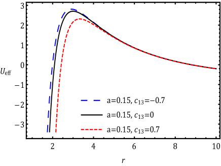
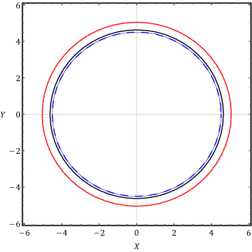
Figure 1: Left graph: The effective potential of the photons $U_{eff}$ as a function of the radial distance $r$, for the Einstein-Æther type I black hole solution (2.26) with (2.13), for various choices of the æther parameter $c_{13}$ and the rotation parameter $a$. Right graph: The corresponding black hole shadow region according to (3.24). In both graphs the $c_{13}$ values have been un-realistically magnified in order to be able to discriminate clearly its effects.

In order to draw the shadow of the BH solution we need to calculate two essential quantities, namely the event horizon radius $r_{e}$ and the radius of the unstable photon sphere $r_{ps}$. In order to find the even horizon of metric (2.13) we have to solve

$$r^{4}-2Mr^{3}-\frac{27c_{13}}{16(1-c_{13})}M^{4}=0~{},$$ (3.25)

which leads to

$$r_{e_{1,2}}=\frac{3M^{2}}{2}-s\pm\frac{1}{2}\sqrt{-4s^{2}+3M^{2}-\frac{M^{2}}{s}},$$ (3.26)

$$r_{e_{3,4}}=\frac{3M^{2}}{2}+s\pm\frac{1}{2}\sqrt{-4s^{2}+3M^{2}+\frac{M^{2}}{s}},$$ (3.27)

where

$$s=\sqrt{\frac{3M^{2}Q+Q^{2}+\Delta_{0}}{12Q}},~{}~{}~{}Q=\left(\frac{\Delta_{1}+\sqrt{\Delta_{1}^{2}-4\Delta_{0}^{3}}}{2}\right)^{1/3},$$ (3.28)

$$\Delta_{0}=-\frac{81c_{13}}{4(1-c_{13})}M^{4},~{}~{}~{}\Delta_{1}=\frac{729c_{13}}{2(1-c_{13})}M^{7}.$$ (3.29)

Solutions $r_{1,2}$ are imaginary and thus not physically interesting. Nevertheless, by setting $c_{13}$ to zero the third solution becomes $r_{3}=2M$, as expected from Schwarzschild background. Thus, we deduce that $r_{3}$ addresses the event horizon radius $r_{e}$ of the Einstein-Æther type I BH solution.

We proceed by setting $\eta=0$, and inserting the $\xi_{ps}$ from $U_{eff}=0$

$$\xi_{ps}=\frac{2Ma}{e(r_{ps})r_{ps}}\left[-1+\sqrt{1+\frac{r_{ps}^{4}e(r_{ps})}{4M^{2}a^{2}}}\right]~{},$$ (3.30)

into (3.17). Then, using $e(r)$ from Eq. (2.13) we finally result to the following equation

$$a^{2}\left(\alpha_{1}-8\right)\left(c_{13}-1\right)r_{ps}^{3}\left[81\alpha_{1}c_{13}+16\left(\alpha_{1}+16\right)\left(c_{13}-1\right)r_{ps}^{4}-48\left(\alpha_{1}+8\right)\left(c_{13}-1\right)r_{ps}^{3}\right]=0~{},$$ (3.31)

with

$$\alpha_{1}=\sqrt{\frac{64a^{2}\left(c_{13}-1\right)(r_{ps}-2)r_{ps}^{3}+16\left(c_{13}-1\right)+27c_{13}}{(c_{13}-1)a^{2}}}~{}.$$ (3.32)

The solution of Eq. (3.31) will provide the radius of the photon sphere $r_{ps}$.

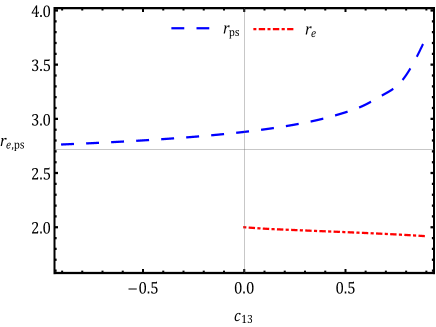
Figure 2: The event horizon radius $r_{e}$ and the radius of the unstable photon sphere $r_{ps}$, in terms of the æther parameter $c_{13}$, for the Einstein-Æther type I black hole solution (2.26) with (2.13), for the representative value $a=0.1$, as they arise by the numerical solution of (3.26) and (3.31) respectively. The interval of the $c_{13}$ values has been un-realistically magnified in order to be able to discriminate clearly its effect.

A first observation is that in the limit $a\rightarrow 0$ Eq. (3.31) reduces to $e^{\prime}(r_{ps})r_{ps}-2e(r_{ps})=0$, as expected [40]. However, in the general case Eqs. (3.26) and (3.31) cannot be solved analytically, and therefore we elaborate them numerically and in Fig. 2 we depict the obtained solutions in terms of the æther parameter $c_{13}$. As one can see, for $c_{13}<0$ the Einstein-Æther type I solution becomes a naked singularity with no event horizon. However, for non-negative $c_{13}$ the photon sphere radius increases, in agreement with the corresponding shift of the peak of $U_{eff}$ in the left panel of Fig. 1. Having in mind the general intuition that for the formation of the shadow the existence of the photon sphere is essential (see however [21] which shows that for a naked singularity there is the possibility of shadow formation without a photon sphere), one could expect that the BH shadow size would be larger than the shadow size of a naked singularity, as depicted in the right panel of Fig. 1. This feature might serve as a phenomenological signal for distinguishing the BH from a naked singularity.

3.2 Einstein-Æther type II black hole solution

In this subsection we perform our analysis for the Einstein-Æther type II black hole solution (2.26), with $e(r)$ given by (2.17). In the left panel of Fig. 3, we depict the effective potential $U_{eff}(r)$ given in (3.15), corresponding to the Einstein-Æther type II BH ($c_{13}\neq 0\neq c_{14}$ but with $c_{123}=0$). As we can see, the behavior of the curves depends on the æther parameters values. In particular, moving from negative to positive values of $c_{13}$ the peak of $U_{eff}$ forms in larger distances with lower height, however, as $c_{14}$ grows (within the allowed interval) the peak moves to lower distances with higher height. Thus, the photon sphere radius will also be different in the various cases.

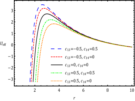
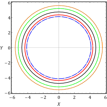
Figure 3: Left graph: The effective potential of the photons $U_{eff}$ as a function of the radial distance $r$, for the Einstein-Æther type II black hole solution (2.26) with (2.17), for various choices of the æther parameters $c_{13}$ and $c_{14}$ and for rotation parameter $a=0.15$. Right graph: The corresponding black hole shadow region according to (3.24). In both graphs the $c_{13}$ and $c_{14}$ values have been un-realistically magnified in order to be able to discriminate clearly their effects.

Similarly to the previous solution subclass above, we can now proceed to the investigation of the resulting event horizon radius $r_{e}$ and of the radius of the unstable photon sphere $r_{ps}$. Using the metric function (2.17), we find $r_{e}$ by solving

$$r^{2}-2Mr-\frac{(2c_{13}-c_{14})M^{2}}{2(1-c_{13})}=0~{},$$ (3.33)

and thus we obtain the two solutions

$$r_{e\mp}=M\bigg{(}1\mp\sqrt{\frac{c_{14}-2}{2c_{13}-2}}\bigg{)}~{}.$$ (3.34)

Amongst them, solution $r_{e+}$ is the physically interesting one, since by setting $c_{13}=0=c_{14}$ this is the one that recovers the general relativity, Schwarzschild result, namely $r_{e}=2M$. Additionally, as one can see, for the allowed values $0<c_{14}<2$ and $c_{13}<1$ the BH has always a real event horizon radius and thus a naked singularities cannot appear, unlike the previous Einstein-Æther type I case.

We proceed by extracting the photon sphere radius. Inserting (3.30) into (3.17) and replacing $e(r)$ from (2.17) we acquire

$$\frac{a^{2}\left(c_{13}-1\right)r_{ps}}{\alpha_{3}{}^{2}}\left\{\left(4-4\alpha_{2}\right){}^{2}\left[2c_{13}(1-r_{ps})+2r_{ps}-c_{14}\right]-\alpha_{3}\left(4-4\alpha_{2}\right){}^{2}-12\alpha_{3}\left(4\alpha_{2}-4\right)\right\}=0,$$ (3.35)

where

$$\alpha_{2}=\sqrt{\frac{r_{ps}^{2}\alpha_{3}}{8a^{2}\left(c_{13}-1\right)}+1}~{},$$

$$\alpha_{3}=-2c_{13}(r_{ps}-1)^{2}+2r(r_{ps}-2)+c_{14}~{}.$$ (3.36)

Similarly to the Einstein-Æther type I case, in the limit $a\rightarrow 0$ Eq. (3.35) also reduces to $e^{\prime}(r_{ps})r_{ps}-2e(r_{ps})=0$, as expected [40].

Since (3.35) cannot be solved analytically, we elaborate it numerically. In the right graph of Fig. 3 we depict the corresponding BH shadow for the same parameter choices of the left graph. As we observe, as the peak of $U_{eff}$ shifts towards smaller (larger) values, the shadow size decreases (increases).

4 The æther parameters $c_{13}$ and $c_{14}$ and M87* observations

We can now proceed to the investigation of the constraints on the æther parameters $c_{13}$ and $c_{14}$ that arise from the EHT Observations of the shadow of M87*. We will focus on the two classes of solutions, namely Einstein-Æther types I and II BH solutions. In particular, observing Figs. 1 and 3 we deduce that the size of the resulting shadow is sensitive on the æther parameters $c_{13}$ and $c_{14}$, and hence the image of M87* is able to impose bounds on them.

In light of the report released by EHT collaboration for the shadow of M87* in [9, 14], for the angular size of the shadow, the mass and the distance to M87* one respectively has the values

$$\delta=(42\pm 3)\,\mu{\text{arcsec}},$$ (4.1)

$$M=(6.5\pm 0.9)\times 10^{9}\,M_{\odot},$$ (4.2)

$$D=16.8^{+0.8}_{-0.7}\,{\text{ Mpc}},$$ (4.3)

where $M_{\odot}$ is the Sun mass. One can merge this information by introducing the single number $d_{M87*}$, which quantifies the size of M87*’s shadow in unit mass, defined as [70]

$$d_{M87*}\equiv\frac{D\delta}{M}\approx 11.0\pm 1.5\,.$$ (4.4)

This combination can be used in order to confront with the theoretically predicted shadows (e.g. the above number is in agreement within $1\sigma$-error with what we theoretically expect for the Schwarzschild BH, namely $d_{Schw}\simeq 10.4$ [25]).

In order to confront Einstein-Æther solutions with the above observational number, all we need is to calculate the angular size $\delta_{I,II}$ for each of the two types of solutions, as a function of the Einstein-Æther parameters. The angular size can be immediately extracted from the profile (3.24), as long as we know the radius of the unstable photon sphere $r_{ps}$ (as a function of the Einstein-Æther parameters). Knowing $\delta_{I,II}$ can then easily lead to the predicted diameter per unit mass $d_{I,II}$ for each of the solutions.

Let us begin our analysis with Einstein-Æther type I BH solution. Note that in agreement with EHT, from now on we fix the value $\theta_{0}=17$ for the inclination angle. In Fig. 4 we depict the diameter of the predicted shadow $d_{I}$ as a function of $c_{13}$ and $a$, on top of the observed one from M87* within $1\sigma$. As we observe, Æther type I BH solution is able to quantitatively describe the shadow size of M87*, provided that the dimensionless spin parameter $a$ is constrained to specific values, dependent on value of $c_{13}$. Note that since our whole analysis has been restricted to the slow rotation case, the extracted upper bounds on $a$ are perfectly consistent and justify our approximation. The curves in Fig. 4 imply that within these ranges of $c_{13}$ it is possible to distinguish a naked singularity ($c_{13}<0$) from BH ($c_{13}>0$). Furthermore, in order to present the bounds on spin parameter $a$ in a more transparent way, we perform a full scan of the two-dimensional parameter space and in Fig. 5 we depict the region which corresponds to a $d_{I}$ in agreement with the observed value $d_{M87*}$. As it is clear from it as well as from the right panel in Fig. 4 , by moving from negative to positive values of æther parameter $c_{13}$, the upper bound on the $a$ grows. This may be useful in distinguishing between BH and naked singularity.

We mention here that in order to create the allowed parameter space plots on the $c_{13}-a$ plane, we have fixed the BH mass to $M=6\times 10^{9}M_{\bigodot}$. Nevertheless, one can also perform a similar parameter scan for the case of non-fixed BH mass, namely within the two-dimensional parameter space $(c_{13},M)$, for different fixed values of the rotation parameter $a$. In Fig. 6 we present such a graph. As we observe, for reasonable $c_{13}$ values, the BH mass lies within the range we expect from EHT for M87*, i.e. $M=(6.5\pm 0.9)\times 10^{9}\,M_{\odot}$. Furthermore, Fig. 6 shows the role of rotation on the allowed region of the $c_{13}-M$ plane, namely by increasing the rotation parameter we are led to larger region for the $c_{13}$ parameter and still be consistent with EHT data within 1-$\sigma$ error. In summary, Einstein-Æther type I BH solution is in agreement with M87* observation, and moreover we obtain a restriction to low rotational values.

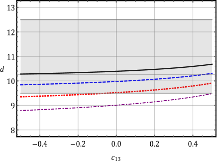
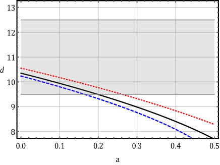
Figure 4: Left graph: The predicted diameter per unit mass $d_{I}$ for the Einstein-Æther type I black hole solution (2.26) with (2.13), as a function of the æther parameter $c_{13}$, for several values of the rotational parameter: $a=0$ (black - solid), $a=0.1$ (blue - dashed), $a=0.2$ (red - dotted), $a=0.3$ (purple - dashed-dotted). Right graph: $d_{I}$ as a function of the rotational parameter $a$, for $c_{13}=-0.5$ (blue - dashed), $c_{13}=0$ (black- solid), $c_{13}=0.5$ (red- dotted). In both graphs the shaded area mark the observationally determined diameter per unit mass of M87*’s shadow, namely $d_{M87*}$, within $1\sigma$-error.

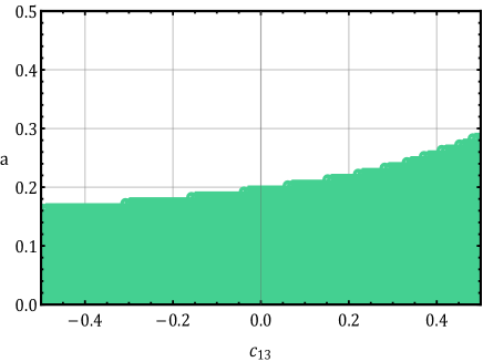
Figure 5: The allowed parameter region ( green) in the $c_{13}-a$ plane, for fixed BH mass ($M=6\times 10^{9}M_{\bigodot}$), for the Einstein-Æther type I black hole solution (2.26) with (2.13), that leads to diameter per unit mass $d_{I}$ in agreement with the observationally determined one $d_{M87*}$ within $1\sigma$-error.

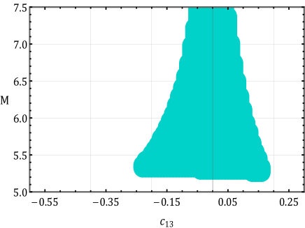
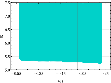
Figure 6: The allowed parameter region (green) in the $c_{13}-M(10^{9}M_{\bigodot})$ plane, for fixed rotation parameter values $a=0$ (left graph) and $a=0.2$ (right graph), for the Einstein-Æther type I black hole solution (2.26) with (2.13), that leads to diameter $d_{I}$ in agreement with the observationally determined one $d_{M87*}$ within $1\sigma$-error.

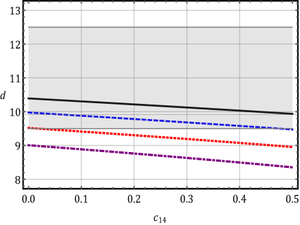
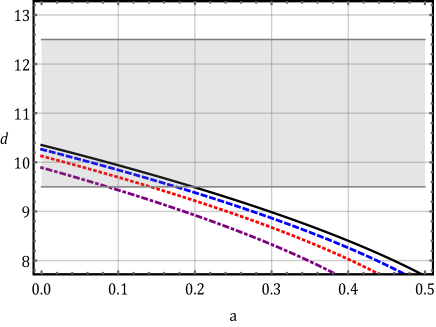
Figure 7: Left graph: The predicted diameter per unit mass $d_{II}$ for the Einstein-Æther type II black hole solution (2.26) with (2.17), as a function of the æther parameter $c_{14}$, for fixed $c_{13}=0$ and for several values of the rotational parameter: $a=0$ (black-solid), $a=0.1$ (blue - dashed), $a=0.2$ (red - dotted), $a=0.3$ (purple - dashed-dotted). Right graph: $d_{II}$ as a function of the rotational parameter $a$, for fixed $c_{13}=0$ and for $c_{14}=0$ (black-solid), $c_{14}=0.1$ (blue - solid), $c_{14}=0.25$ (red - dotted), $c_{14}=0.5$ (purple - dashed-dotted). In both graphs the shaded area mark the observationally determined diameter per unit mass of M87*’s shadow, namely $d_{M87*}$, within $1\sigma$-error.

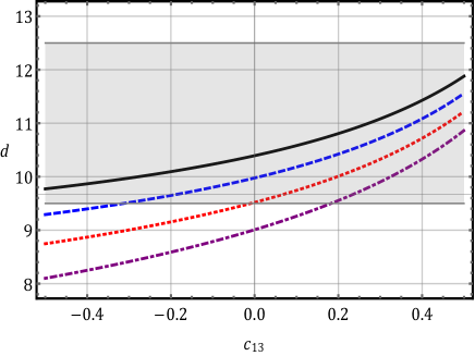
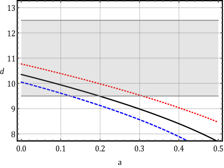
Figure 8: Left graph: The predicted diameter per unit mass $d_{II}$ for the Einstein-Æther type II black hole solution (2.26) with (2.17), as a function of the æther parameter $c_{13}$, for fixed $c_{14}=0$ and for several values of the rotational parameter: $a=0$ (black-solid), $a=0.1$ (blue - dashed), $a=0.2$ (red - dotted), $a=0.3$ (purple - dashed-dotted). Right graph: $d_{II}$ as a function of the rotational parameter $a$, for fixed $c_{14}=0$ and for $c_{13}=0$ (black-solid), $c_{13}=-0.2$ (blue - solid), $c_{13}=0.2$ (red - dotted). In both graphs the shaded area mark the observationally determined diameter per unit mass of M87*’s shadow, namely $d_{M87*}$, within $1\sigma$-error.

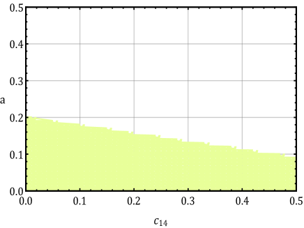
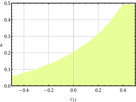
Figure 9: The allowed parameter regions (light green) in the $c_{14}-a$ and $c_{13}-a$ planes, for fixed BH mass ($M=6\times 10^{9}M_{\bigodot}$), for the Einstein-Æther type II black hole solution (2.26) with (2.17), that leads to diameter per unit mass $d_{II}$ in agreement with the observationally determined one $d_{M87*}$ within $1\sigma$-error.

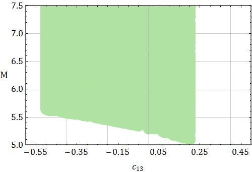
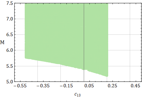
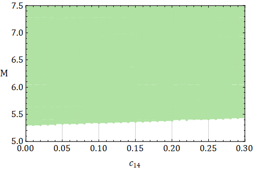
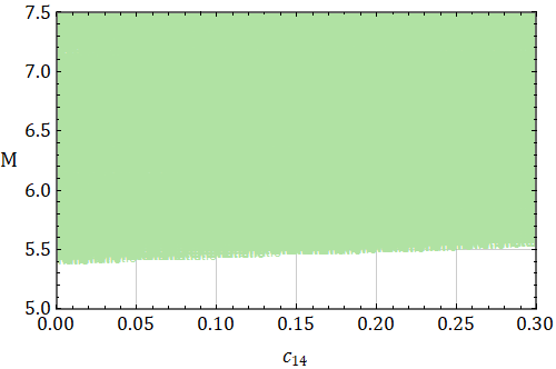
Figure 10: The allowed parameter regions (green) in the $c_{13}-M(10^{9}M_{\bigodot})$ plane (upper graphs) and $c_{14}-M(10^{9}M_{\bigodot})$ planes (lower graphs), for fixed rotation parameter values $a=0$ (left graphs) and $a=0.2$ (right graphs), for the Einstein-Æther type II black hole solution (2.26) with (2.17), that leads to diameter $d_{II}$ in agreement with the observationally determined one $d_{M87*}$ within $1\sigma$-error.

We proceed to the investigation of the Einstein-Æther type II BH solution, which involves the æther parameters $c_{13}$ and $c_{14}$. In Figs. 7 and 8 we respectively draw the diameter of the predicted shadow as a function of $c_{14}$, $a$ and $c_{13}$, $a$, on top of the observed one from M87* within $1\sigma$-error. Similarly to the previous case, we deduce that we obtain agreement with the observed behavior if the involved æther parameters are restricted within a given range, along with an upper bound on $a$. Concerning the æther parameter $c_{14}$, as it increases then the upper bound on $a$ decreases, while for the parameter $c_{13}$ this $a$-behavior happens by moving from positive values to negative value. Additionally, the restriction of the rotation parameter $a$ to a given narrow window can also be extracted by scanning the two-dimensional spaces $(c_{14},a)$ and $(c_{13},a)$, for fixed BH mass, as depicted in Fig. 9. Note that the above statement on the change of trend of æther parameters and rotation parameter, can also be verified through Fig. 9, too. Finally, note that such small $a$ values verify that our slow rotation approximation is indeed valid.

Similarly to the Einstein-Æther type I black hole solution, in the present type II solutions we can also provide two-dimensional scans on the planes $c_{13}-M$ and $c_{14}-M$, for fixed rotation parameters. As we observe in Fig. 10, unlike the type I solution case, in the present Einstein-Æther type II black hole solutions the rotation parameter does not play a significant role in reducing the allowed parameter space. Moreover, the BH mass can be matched with what extracted by EHT for M87* within $1\sigma$-error.

We close this section by making some comments on the rotation behavior. It is known that one might have degeneracies of additional parameters in general relativity - magnetohydrodynamic (GR-MHD) simulations, which could allow for high spin values, namely $a>0.5$ [13]. In particular, since spin can be a strong energy source for powering relativistic jets, one could have the case where high spin values in specific GR-MHD models could produce powerful jets. The estimates of M87’s jet power lie in the range $10^{42}$ to $10^{45}erg/s$ [133, 134, 135], with values closer to $10^{42}$ being favored, as it is observed form Table 3 of [13]. Additionally, it is expected that the value of the real jet power could be higher than $10^{42}erg/s$ (for instance observations of Hubble Space Telescope (HST)-1 [136] and Low-Frequency Array (LOFAR) [134] yield $\sim 10^{44}erg/s$). Hence, although GR-MHD simulations reveal that most of high spin models can produce sufficiently powerful jets ($E>10^{42}erg/s$) and thus they can satisfy the lower limit of the power jets, they could still have no perfect agreement with the actual upper values. We mention here that the jet formation mechanism in our scenario is the same with the case of general relativity, i.e we do not use modified gravity as an explanation of the jet formation. A full MHD simulation in modified gravity would be both necessary and interesting, nevertheless it lies beyond the scope of the present work. In general, future high-fidelity interferometric imaging of M87* and/or Sgr A*, are expected to clarify the role and value of spin.

For the moment it is adequate to resort to different probes of the BH rotation rate, such as X-ray reflection spectroscopy. In general, although observational data indicate the existence of rotating BHs, there is no quantitative consensus and the literature contains a variety of constraints [137, 138]. For instance it remains an open issue whether the astrophysical BHs have slow, modest or rapid rotational behavior. Concerning supermassive BHs, the corresponding information is obtained through the relativistic X-ray reflection spectroscopy, which is a powerful technique applicable to measure robust BH spins across the mass range, from the stellar-mass BHs in X-ray binaries to the supermassive BHs in active galactic nuclei (AGN) [137, 138]. By utilizing this method within recent structure formation models, one might face a mass dependency for the distribution of supermassive BH spins [139, 140, 141, 142]. However, an important point to note is that the X-ray reflection technique should be used only for the standard accretion disk case, i.e. for moderate mass accretion rates in the range $\dot{M}\sim 0.01-0.3\dot{M}_{Edd}$, with $\dot{M}_{Edd}$ the Eddington mass accretion rate [137]. Although it is expected that this technique is applicable for BH X-ray binaries in their luminous hard state, it cannot work for the low-luminosity type of AGNs like M87* and Sgr A*, since the corresponding accretion rate is very low.

5 Conclusions

In the present work we investigated Einstein-Æther gravity in light of the recent Event Horizon Telescope (EHT) observations of the M87*. In particular, the EHT provided the first visual evidence indicating directly the existence of a compact object such as a supermassive black hole (BH) candidate at the center of the M87* galaxy. Since the shape and size of the observed BH shadow contains information of the geometry in the vicinity of the BH, one can consider the shadow as a potential probe to investigate the BH structure within different gravitational theories, due to the fact that in modified gravity one obtain black holes which deviate from those of general relativity. Hence, allowing for a modified gravity as the underlying theory enriches the calculation framework with different size-rotation features as well as with extra model parameters.

The Einstein-Æther (EA) theory is a generally covariant theory of gravity, which violates the Lorentz invariance locally by possessing a dynamical, unit-norm and timelike vector field, namely the æther field, which defines a preferred timelike direction at each spacetime point. The black hole solutions in such a framework include two classes of slow rotating spherically symmetric solutions, depending on the involved mixed æther parameters $c_{13}$ and $c_{14}$.

We first extracted the above black hole solutions for EA gravity, and we calculated the corresponding effective potential $U_{eff}(r)$ for the photons, the resulting event horizon radius $r_{e}$ and the radius of the unstable photon sphere $r_{ps}$. Then we straightforwardly calculated the induced angular size $\delta$, which combined with the mass and the distance can lead to a single prediction that quantifies the black hole shadow size, namely the diameter per unit mass $d$. Since $d_{M87*}$ is observationally known from the EHT Probe, we extracted the corresponding parameter regions of instein-Æther theory in order to obtain consistency.

Apart from the restriction of the æther parameters $c_{13}$ and $c_{14}$ to specif ranges, we found some constraints on the dimensionless spin parameter $a$ in slow rotation limit, dependent on the values of æther parameters, which was verified by a full scan of the parameter space. Furthermore, our analysis has indicated that in the Einstein-Æther (EA) theory (type I BH solution) is possible to distinguish a naked singularity from BH. This is indeed a verification of the fact that in modified gravity one obtains different size-rotation features, depending on the extra model parameters, and hence the M87* observation can be in principle described in different ways comparing to general relativity, especially in theories which possess various corrections on the Kerr-metric solutions, such is the case in Einstein-Æther gravity.

In summary, Einstein-Æther black hole solutions are in agreement with EHT M87* observation, and this may act as an advantage for Einstein-Æther gravity.

References

- [1] N. I. Shakura and R. A. Sunyaev, Black holes in binary systems. Observational appearance, Astron. Astrophys. 24, 337 (1973).
- [2] B. P. Abbott et al. [LIGO Scientific and Virgo Collaborations], Observation of Gravitational Waves from a Binary Black Hole Merger, Phys. Rev. Lett. 116, no. 6, 061102 (2016) [arXiv:1602.03837].
- [3] B. P. Abbott et al. [LIGO Scientific and Virgo Collaborations], GW151226: Observation of Gravitational Waves from a 22-Solar-Mass Binary Black Hole Coalescence, Phys. Rev. Lett. 116, no. 24, 241103 (2016) [arXiv:1606.04855].
- [4] B. P. Abbott et al. [LIGO Scientific and VIRGO Collaborations], GW170104: Observation of a 50-Solar-Mass Binary Black Hole Coalescence at Redshift 0.2, Phys. Rev. Lett. 118, no. 22, 221101 (2017) Erratum: [Phys. Rev. Lett. 121, no. 12, 129901 (2018)] [arXiv:1706.01812].
- [5] B. P. Abbott et al. [LIGO Scientific and Virgo Collaborations], GW170814: A Three-Detector Observation of Gravitational Waves from a Binary Black Hole Coalescence, Phys. Rev. Lett. 119, no. 14, 141101 (2017) [arXiv:1709.09660].
- [6] B. . P. .Abbott et al. [LIGO Scientific and Virgo Collaborations], GW170608: Observation of a 19-solar-mass Binary Black Hole Coalescence, Astrophys. J. Lett. 851, L35 (2017) [arXiv:1711.05578].
- [7] B. P. Abbott et al. [LIGO Scientific and Virgo Collaborations], GW170817: Observation of Gravitational Waves from a Binary Neutron Star Inspiral, Phys. Rev. Lett. 119, no. 16, 161101 (2017) [arXiv:1710.05832].
- [8] B. P. Abbott et al. [LIGO Scientific and Virgo and Fermi-GBM and INTEGRAL Collaborations], Gravitational Waves and Gamma-rays from a Binary Neutron Star Merger: GW170817 and GRB 170817A, Astrophys. J. Lett. 848, no. 2, L13 (2017) [arXiv:1710.05834].
- [9] K. Akiyama et al. [Event Horizon Telescope Collaboration], First M87 Event Horizon Telescope Results. I. The Shadow of the Supermassive Black Hole, Astrophys. J. Lett. 875, L1 (2019) [arXiv:1906.11238].
- [10] K. Akiyama et al. [Event Horizon Telescope Collaboration], First M87 Event Horizon Telescope Results. II. Array and Instrumentation, Astrophys. J. Lett. 875, no. 1, L2 (2019) [arXiv:1906.11239].
- [11] K. Akiyama et al. [Event Horizon Telescope Collaboration], First M87 Event Horizon Telescope Results. III. Data Processing and Calibration, Astrophys. J. Lett. 875, no. 1, L3 (2019) [arXiv:1906.11240].
- [12] K. Akiyama et al. [Event Horizon Telescope Collaboration], First M87 Event Horizon Telescope Results. IV. Imaging the Central Supermassive Black Hole, Astrophys. J. Lett. 875, no. 1, L4 (2019) [arXiv:1906.11241].
- [13] K. Akiyama et al. [Event Horizon Telescope Collaboration], First M87 Event Horizon Telescope Results. V. Physical Origin of the Asymmetric Ring, Astrophys. J. Lett. 875, no. 1, L5 (2019) [arXiv:1906.11242].
- [14] K. Akiyama et al. [Event Horizon Telescope Collaboration], First M87 Event Horizon Telescope Results. VI. The Shadow and Mass of the Central Black Hole, Astrophys. J. Lett. 875, no. 1, L6 (2019) [arXiv:1906.11243].
- [15] T. Ohgami and N. Sakai, Wormhole shadows, Phys. Rev. D 91, no. 12, 124020 (2015) [arXiv:1704.07065].
- [16] R. Shaikh, Shadows of rotating wormholes, Phys. Rev. D 98, no. 2, 024044 (2018) [arXiv:1803.11422].
- [17] K. S. Virbhadra and G. F. R. Ellis, Gravitational lensing by naked singularities, Phys. Rev. D 65, 103004 (2002).
- [18] K. S. Virbhadra and C. R. Keeton, Time delay and magnification centroid due to gravitational lensing by black holes and naked singularities, Phys. Rev. D 77, 124014 (2008) [arXiv:0710.2333].
- [19] N. Ortiz, O. Sarbach and T. Zannias, Shadow of a naked singularity, Phys. Rev. D 92, no. 4, 044035 (2015) [arXiv:1505.07017].
- [20] R. Shaikh, P. Kocherlakota, R. Narayan and P. S. Joshi, Shadows of spherically symmetric black holes and naked singularities, Mon. Not. Roy. Astron. Soc. 482, no. 1, 52 (2019) [arXiv:1802.08060].
- [21] A. B. Joshi, D. Dey, P. S. Joshi and P. Bambhaniya, Shadow of a Naked Singularity without Photon Sphere, Phys. Rev. D 102, no. 2, 024022 (2020) [arXiv:2004.06525].
- [22] A. E. Broderick, A. Loeb and R. Narayan, The Event Horizon of Sagittarius A*, Astrophys. J. 701, 1357 (2009) [arXiv:0903.1105].
- [23] C. Bambi, A note on the observational evidence for the existence of event horizons in astrophysical black hole candidates, Scientific World Journal 2013, 204315 (2013) [arXiv:1205.4640].
- [24] P. V. P. Cunha and C. A. R. Herdeiro, Shadows and strong gravitational lensing: a brief review, Gen. Rel. Grav. 50, no. 4, 42 (2018) [arXiv:1801.00860].
- [25] S. Chandrasekhar, The mathematical theory of black holes, Oxford classic texts in the physical sciences, Oxford Univ. Press, Oxford (2002).
- [26] J. L. Synge, The Escape of Photons from Gravitationally Intense Stars, Mon. Not. Roy. Astron. Soc. 131, no. 3, 463 (1966).
- [27] J.-P. Luminet, Image of a spherical black hole with thin accretion disk, Astron. Astrophys. 75, 228 (1979).
- [28] J. M. Bardeen, Timelike and null geodesics of the Kerr metric, Gordon Breach, Science Publishers, New York (1973).
- [29] R. Narayan, M. D. Johnson and C. F. Gammie, The Shadow of a Spherically Accreting Black Hole, Astrophys. J. Lett. 885, no. 2, L33 (2019) [arXiv:1910.02957].
- [30] H. Falcke, F. Melia and E. Agol, Viewing the shadow of the black hole at the galactic center, Astrophys. J. Lett. 528, L13 (2000) [arXiv:astro-ph/9912263].
- [31] Z. Younsi, A. Zhidenko, L. Rezzolla, R. Konoplya and Y. Mizuno, New method for shadow calculations: Application to parametrized axisymmetric black holes, Phys. Rev. D 94, no. 8, 084025 (2016) [arXiv:1607.05767].
- [32] Y. Mizuno, Z. Younsi, C. M. Fromm, O. Porth, M. De Laurentis, H. Olivares, H. Falcke, M. Kramer and L. Rezzolla, The Current Ability to Test Theories of Gravity with Black Hole Shadows, Nature Astron. 2, no. 7, 585 (2018) [arXiv:1804.05812].
- [33] V. De Falco, E. Battista, S. Capozziello and M. De Laurentis, Testing wormhole solutions in extended gravity through the Poynting-Robertson effect, Phys. Rev. D 103, no. 4, 044007 (2021) [ arXiv:2101.04960].
- [34] R. Shaikh, Black hole shadow in a general rotating spacetime obtained through Newman-Janis algorithm, Phys. Rev. D 100, no. 2, 024028 (2019) [arXiv:1904.08322].
- [35] S. W. Wei, Y. C. Zou, Y. X. Liu and R. B. Mann, Curvature radius and Kerr black hole shadow, JCAP 1908, 030 (2019) [arXiv:1904.07710].
- [36] J. W. Moffat and V. T. Toth, Masses and shadows of the black holes Sagittarius A* and M87* in modified gravity, Phys. Rev. D 101, no. 2, 024014 (2020) [arXiv:1904.04142].
- [37] J. T. Firouzjaee and A. Allahyari, Black hole shadow with a cosmological constant for cosmological observers, Eur. Phys. J. C 79, no. 11, 930 (2019) [arXiv:1905.07378].
- [38] I. Banerjee, B. Mandal and S. SenGupta, Does black hole continuum spectrum signal gravity in higher dimensions?, Phys. Rev. D 101, no. 2, 024013 (2020) [arXiv:1905.12820].
- [39] F. Long, J. Wang, S. Chen and J. Jing, Shadow of a rotating squashed Kaluza-Klein black hole, JHEP 1910, 269 (2019) [arXiv:1906.04456].
- [40] T. Zhu, Q. Wu, M. Jamil and K. Jusufi, Shadows and deflection angle of charged and slowly rotating black holes in Einstein-Æther theory, Phys. Rev. D 100, no. 4, 044055 (2019) [arXiv:1906.05673].
- [41] R. A. Konoplya and A. Zhidenko, Analytical representation for metrics of scalarized Einstein-Maxwell black holes and their shadows, Phys. Rev. D 100, no. 4, 044015 (2019) [arXiv:1907.05551].
- [42] E. Contreras, Á. Rincón, G. Panotopoulos, P. Bargueño and B. Koch, Black hole shadow of a rotating scale–dependent black hole, Phys. Rev. D 101, no. 6, 064053 (2020) [arXiv:1906.06990].
- [43] P. C. Li, M. Guo and B. Chen, Shadow of a Spinning Black Hole in an Expanding Universe, Phys. Rev. D 101, no. 8, 084041 (2020) [arXiv:2001.04231].
- [44] R. Kumar, S. G. Ghosh and A. Wang, Gravitational deflection of light and shadow cast by rotating Kalb-Ramond black holes, Phys. Rev. D 101, no. 10, 104001 (2020) [arXiv:2001.00460].
- [45] R. C. Pantig and E. T. Rodulfo, Rotating dirty black hole and its shadow, Chin. J. Phys. 68, 236 (2020) [arXiv:2003.06829].
- [46] S. V. M. C. B. Xavier, P. V. P. Cunha, L. C. B. Crispino and C. A. R. Herdeiro, Shadows of charged rotating black holes: Kerr–Newman versus Kerr–Sen, Int. J. Mod. Phys. D 29, no. 11, 2041005 (2020) [arXiv:2003.14349].
- [47] M. Guo and P. C. Li, Innermost stable circular orbit and shadow of the Einstein–Gauss–Bonnet black hole, Eur. Phys. J. C 80, no. 6, 588 (2020) [arXiv:2003.02523].
- [48] R. Roy and S. Chakrabarti, Study on black hole shadows in asymptotically de Sitter spacetimes, Phys. Rev. D 102, no. 2, 024059 (2020) [arXiv:2003.14107].
- [49] X. H. Jin, Y. X. Gao and D. J. Liu, Strong gravitational lensing of a 4-dimensional Einstein–Gauss–Bonnet black hole in homogeneous plasma, Int. J. Mod. Phys. D 29, no. 09, 2050065 (2020) [arXiv:2004.02261].
- [50] S. U. Islam, R. Kumar and S. G. Ghosh, Gravitational lensing by black holes in the Einstein-Gauss-Bonnet gravity, JCAP 2009, 030 (2020) [arXiv:2004.01038].
- [51] C. Y. Chen, Rotating black holes without symmetry and their shadow images, JCAP 05, 040 (2020) [arXiv:2004.01440].
- [52] X. X. Zeng and H. Q. Zhang, Influence of quintessence dark energy on the shadow of black hole, Eur. Phys. J. C 80, no.11, 1058, [arXiv:2007.06333].
- [53] R. A. Konoplya, J. Schee and D. Ovchinnikov, Shadow of the magnetically and tidally deformed black hole, [arXiv:2008.04118].
- [54] A. Belhaj, M. Benali, A. E. Balali, W. E. Hadri, H. El Moumni and E. Torrente-Lujan, Black Hole Shadows in M-theory Scenarios, [arXiv:2008.09908].
- [55] F. Long, S. Chen, M. Wang and J. Jing, Shadow of a disformal Kerr black hole in quadratic DHOST theories, [arXiv:2009.07508].
- [56] K. Jusufi and Saurabh, Black Hole Shadows in Verlinde’s Emergent Gravity, [arXiv:2010.15870].
- [57] E. Contreras, Á. Rincón, G. Panotopoulos and P. Bargueño, Geodesic analysis and black hole shadows on a general non–extremal rotating black hole in five–dimensional gauged supergravity, [arXiv:2010.03734].
- [58] W. H. Shao, C. Y. Chen and P. Chen, Generating Rotating Spacetime in Ricci-Based Gravity: Naked Singularity as a Black Hole Mimicker, [arXiv:2011.07763].
- [59] S. G. Ghosh, R. Kumar and S. U. Islam, Parameters estimation and strong gravitational lensing of nonsingular Kerr-Sen black holes, [arXiv:2011.08023].
- [60] H. Davoudiasl and P. B. Denton, Ultralight Boson Dark Matter and Event Horizon Telescope Observations of M87*, Phys. Rev. Lett. 123, no. 2, 021102 (2019) [arXiv:1904.09242].
- [61] N. Bar, K. Blum, T. Lacroix and P. Panci, Looking for ultralight dark matter near supermassive black holes, JCAP 1907, 045 (2019) [arXiv:1905.11745].
- [62] K. Jusufi, M. Jamil, P. Salucci, T. Zhu and S. Haroon, Black Hole Surrounded by a Dark Matter Halo in the M87 Galactic Center and its Identification with Shadow Images, Phys. Rev. D 100, no. 4, 044012 (2019) [arXiv:1905.11803].
- [63] R. A. Konoplya, Shadow of a black hole surrounded by dark matter, Phys. Lett. B 795, 1 (2019) [arXiv:1905.00064].
- [64] A. Narang, S. Mohanty and A. Kumar, Test of Kerr-Sen metric with black hole observations, [arXiv:2002.12786].
- [65] S. Sau, I. Banerjee and S. SenGupta, Imprints of the Janis-Newman-Winicour spacetime on observations related to shadow and accretion, Phys. Rev. D 102, no. 6, 064027 (2020) [arXiv:2004.02840].
- [66] A. Belhaj, M. Benali, A. El Balali, H. El Moumni and S. E. Ennadifi, Deflection angle and shadow behaviors of quintessential black holes in arbitrary dimensions, Class. Quant. Grav. 37, no. 21, 215004 (2020) [arXiv:2006.01078].
- [67] R. Kumar, A. Kumar and S. G. Ghosh, Testing Rotating Regular Metrics as Candidates for Astrophysical Black Holes, Astrophys. J. 896, no. 1, 89 (2020) [arXiv:2006.09869].
- [68] X. X. Zeng and H. Q. Zhang, Influence of quintessence dark energy on the shadow of black hole, Eur. Phys. J. C 80, no. 11, 1058 [arXiv:2007.06333].
- [69] Saurabh and K. Jusufi, Imprints of Dark Matter on Black Hole Shadows using Spherical Accretions, [arXiv:2009.10599].
- [70] C. Bambi, K. Freese, S. Vagnozzi and L. Visinelli, Testing the rotational nature of the supermassive object M87* from the circularity and size of its first image, Phys. Rev. D 100, no. 4, 044057 (2019) [arXiv:1904.12983].
- [71] S. Vagnozzi and L. Visinelli, Hunting for extra dimensions in the shadow of M87*, Phys. Rev. D 100, no. 2, 024020 (2019) [arXiv:1905.12421].
- [72] S. Haroon, K. Jusufi and M. Jamil, Shadow Images of a Rotating Dyonic Black Hole with a Global Monopole Surrounded by Perfect Fluid, Universe 6, no. 2, 23 (2020) [arXiv:1904.00711].
- [73] R. Shaikh and P. S. Joshi, Can we distinguish black holes from naked singularities by the images of their accretion disks?, JCAP 1910, 064 (2019) [arXiv:1909.10322].
- [74] P. V. P. Cunha, C. A. R. Herdeiro and E. Radu, EHT constraint on the ultralight scalar hair of the M87 supermassive black hole, Universe 5, no. 12, 220 (2019) [arXiv:1909.08039].
- [75] I. Banerjee, S. Chakraborty and S. SenGupta, Silhouette of M87*: A New Window to Peek into the World of Hidden Dimensions, Phys. Rev. D 101, no. 4, 041301 (2020) [arXiv:1909.09385].
- [76] X. H. Feng and H. Lu, On the size of rotating black holes, Eur. Phys. J. C 80, no. 6, 551 (2020) [arXiv:1911.12368].
- [77] S. F. Yan, C. Li, L. Xue, X. Ren, Y. F. Cai, D. A. Easson, Y. F. Yuan and H. Zhao, Testing the equivalence principle via the shadow of black holes, Phys. Rev. Res. 2, no. 2, 023164 (2020) [arXiv:1912.12629].
- [78] A. Allahyari, M. Khodadi, S. Vagnozzi and D. F. Mota, Magnetically charged black holes from non-linear electrodynamics and the Event Horizon Telescope, JCAP 2002, 003 (2020) [arXiv:1912.08231].
- [79] M. Rummel and C. P. Burgess, Constraining Fundamental Physics with the Event Horizon Telescope, JCAP 2005, 051 (2020) [arXiv:2001.00041].
- [80] S. Vagnozzi, C. Bambi and L. Visinelli, Concerns regarding the use of black hole shadows as standard rulers, Class. Quant. Grav. 37, no. 8, 087001 (2020) [arXiv:2001.02986].
- [81] M. Khodadi, A. Allahyari, S. Vagnozzi and D. F. Mota, Black holes with scalar hair in light of the Event Horizon Telescope, JCAP 2009, 026 (2020) [arXiv:2005.05992].
- [82] Z. Chang and Q. H. Zhu, Does the shape of the shadow of a black hole depend on motional status of an observer?, Phys. Rev. D 102, no. 4, 044012 (2020) [arXiv:2006.00685].
- [83] S. I. Kruglov, The shadow of M87* black hole within rational nonlinear electrodynamics, Mod. Phys. Lett. A 35, no. 35, 2050291 (2020).
- [84] D. Ghosh, A. Thalapillil and F. Ullah, Astrophysical hints for magnetic black holes, [arXiv:2009.03363].
- [85] D. Psaltis et al. [Event Horizon Telescope Collaboration], Gravitational Test Beyond the First Post-Newtonian Order with the Shadow of the M87 Black Hole, Phys. Rev. Lett. 125, no. 14, 141104 (2020) [arXiv:2010.01055].
- [86] K. Jusufi, Quasinormal Modes of Black Holes Surrounded by Dark Matter and Their Connection with the Shadow Radius, Phys. Rev. D 101, no. 8, 084055 (2020) [arXiv:1912.13320].
- [87] R. Kumar, S. G. Ghosh and A. Wang, Shadow cast and deflection of light by charged rotating regular black holes, Phys. Rev. D 100, no. 12, 124024 (2019) [arXiv:1912.05154].
- [88] R. A. Konoplya and A. F. Zinhailo, Quasinormal modes, stability and shadows of a black hole in the 4D Einstein–Gauss–Bonnet gravity, Eur. Phys. J. C 80, no. 11, 1049 (2020) [arXiv:2003.01188].
- [89] C. Liu, T. Zhu, Q. Wu, K. Jusufi, M. Jamil, M. Azreg-Aïnou and A. Wang, Shadow and Quasinormal Modes of a Rotating Loop Quantum Black Hole, Phys. Rev. D 101, no. 8, 084001 (2020) [arXiv:2003.00477].
- [90] K. Jusufi, Connection Between the Shadow Radius and Quasinormal Modes in Rotating Spacetimes, Phys. Rev. D 101, no. 12, 124063 (2020) [arXiv:2004.04664].
- [91] K. Jusufi, M. Amir, M. S. Ali and S. D. Maharaj, Quasinormal modes, shadow and greybody factors of 5D electrically charged Bardeen black holes, Phys. Rev. D 102, no. 6, 064020 (2020) [arXiv:2005.11080].
- [92] K. Jusufi, M. Azreg-Aïnou, M. Jamil, S. W. Wei, Q. Wu and A. Wang, Quasinormal modes, quasiperiodic oscillations and shadow of rotating regular black holes in non-minimally coupled Einstein-Yang-Mills theory, [arXiv:2008.08450].
- [93] M. Ghasemi-Nodehi, M. Azreg-Aïnou, K. Jusufi and M. Jamil, Shadow, quasinormal modes, and quasiperiodic oscillations of rotating Kaluza-Klein black holes, Phys. Rev. D 102, no. 10, 104032 (2020) [arXiv:2011.02276].
- [94] H. Olivares, O. Porth, J. Davelaar, E. R. Most, C. M. Fromm, Y. Mizuno, Z. Younsi and L. Rezzolla, Constrained transport and adaptive mesh refinement in the Black Hole Accretion Code, Astron. Astrophys. 629, A61 (2019) [ arXiv:1906.10795].
- [95] C. J. White, Development and Application of Numerical Techniques for General-Relativistic Magnetohydrodynamics Simulations of Black Hole Accretion, [arXiv:1906.09708].
- [96] A. Nathanail, C. M. Fromm, O. Porth, H. Olivares, Z. Younsi, Y. Mizuno and L. Rezzolla, Plasmoid formation in global GRMHD simulations and AGN flares, Mon. Not. Roy. Astron. Soc. 495, no. 2, 1549 (2020) [arXiv:2002.01777].
- [97] T. Bronzwaer, J. Davelaar, Z. Younsi, M. Mościbrodzka, H. Olivares, Y. Mizuno, J. Vos and H. Falcke, Visibility of Black Hole Shadows in Low-luminosity AGN, Mon. Not. Roy. Astron. Soc. 501, no. 4, 4722 (2021) [arXiv:2011.00069].
- [98] A. Cruz-Osorio, S. Gimeno-Soler, J. A. Font, M. De Laurentis and S. Mendoza, Magnetized discs and photon rings around Yukawa-like black holes, [arXiv:2102.10150].
- [99] D. Mattingly, Modern tests of Lorentz invariance, Living Rev. Rel. 8, 5 (2005) [arXiv:gr-qc/0502097].
- [100] C. M. Will, The Confrontation between general relativity and experiment, Living Rev. Rel. 9, 3 (2006) [arXiv:gr-qc/0510072].
- [101] S. Liberati, Lorentz symmetry breaking: phenomenology and constraints, J. Phys. Conf. Ser. 631, no. 1, 012011 (2015).
- [102] D. Colladay and V. A. Kostelecky, Lorentz violating extension of the standard model, Phys. Rev. D 58, 116002 (1998) [arXiv:hep-ph/9809521].
- [103] V. A. Kostelecky, Gravity, Lorentz violation, and the standard model, Phys. Rev. D 69, 105009 (2004) [arXiv:hep-th/0312310].
- [104] T. Jacobson and D. Mattingly, Gravity with a dynamical preferred frame, Phys. Rev. D 64, 024028 (2001) [arXiv:gr-qc/0007031].
- [105] C. Eling, T. Jacobson and D. Mattingly, Einstein-Æther theory, [arXiv:gr-qc/0410001].
- [106] T. Jacobson, Einstein-Æther gravity: A Status report, PoS QG -PH, 020 (2007) [arXiv:0801.1547].
- [107] B. Z. Foster and T. Jacobson, Post-Newtonian parameters and constraints on Einstein-Æther theory, Phys. Rev. D 73, 064015 (2006) [arXiv:gr-qc/0509083].
- [108] J. W. Elliott, G. D. Moore and H. Stoica, Constraining the new Aether: Gravitational Cerenkov radiation, JHEP 0508, 066 (2005) [arXiv:hep-ph/0505211].
- [109] B. Li, D. Fonseca Mota and J. D. Barrow, Detecting a Lorentz-Violating Field in Cosmology, Phys. Rev. D 77, 024032 (2008) [arXiv:0709.4581].
- [110] K. Yagi, D. Blas, E. Barausse and N. Yunes, Constraints on Einstein-Æther theory and Hořava gravity from binary pulsar observations, Phys. Rev. D 89, no. 8, 084067 (2014) Erratum: [Phys. Rev. D 90, no. 6, 069902 (2014)] Erratum: [Phys. Rev. D 90, no. 6, 069901 (2014)] [arXiv:1311.7144].
- [111] P. Horava, Quantum Gravity at a Lifshitz Point, Phys. Rev. D 79, 084008 (2009) [arXiv:0901.3775].
- [112] S. Mukohyama, Horava-Lifshitz Cosmology: A Review, Class. Quant. Grav. 27, 223101 (2010) [arXiv:1007.5199].
- [113] A. Wang, Horava gravity at a Lifshitz point: A progress report, Int. J. Mod. Phys. D 26, 1730014 (2017), [arXiv:1701.06087].
- [114] A. H. Chamseddine and V. Mukhanov, Mimetic Dark Matter, JHEP 1311, 135 (2013) [arXiv:1308.5410].
- [115] A. H. Chamseddine, V. Mukhanov and A. Vikman, Cosmology with Mimetic Matter, JCAP 1406, 017 (2014) [arXiv:1403.3961].
- [116] S. Basilakos, A. P. Kouretsis, E. N. Saridakis and P. Stavrinos, Resembling dark energy and modified gravity with Finsler-Randers cosmology, Phys. Rev. D 88, 123510 (2013) [arXiv:1311.5915].
- [117] S. Ikeda, E. N. Saridakis, P. C. Stavrinos and A. Triantafyllopoulos, Cosmology of Lorentz fiber-bundle induced scalar-tensor theories, Phys. Rev. D 100, no.12, 124035 (2019) [arXiv:1907.10950].
- [118] L. Sebastiani, S. Vagnozzi and R. Myrzakulov, Mimetic gravity: a review of recent developments and applications to cosmology and astrophysics, Adv. High Energy Phys. 2017, 3156915 (2017) [arXiv:1612.08661].
- [119] J. Oost, S. Mukohyama and A. Wang, Constraints on Einstein-Æther theory after GW170817, Phys. Rev. D 97, no. 12, 124023 (2018) [arXiv:1802.04303].
- [120] C. Eling and T. Jacobson, Black Holes in Einstein-Æther Theory, Class. Quant. Grav. 23, 5643 (2006) Erratum: [Class. Quant. Grav. 27, 049802 (2010)] [arXiv:gr-qc/0604088].
- [121] E. Barausse, T. Jacobson and T. P. Sotiriou, Black holes in Einstein-Æther and Horava-Lifshitz gravity, Phys. Rev. D 83, 124043 (2011) [arXiv:1104.2889].
- [122] C. Ding, A. Wang and X. Wang, Charged Einstein-Æther black holes and Smarr formula, Phys. Rev. D 92, no. 8, 084055 (2015) [arXiv:1507.06618].
- [123] C. Zhang, X. Zhao, K. Lin, S. Zhang, W. Zhao and A. Wang, Spherically symmetric static black holes in Einstein-aether theory, Phys. Rev. D 102, no.6, 064043 (2020) [arXiv:2004.06155].
- [124] D. Psaltis, F. Ozel, C. K. Chan and D. P. Marrone, A General Relativistic Null Hypothesis Test with Event Horizon Telescope Observations of the black-hole shadow in Sgr A*, Astrophys. J. 814, no. 2, 115 (2015) [arXiv:1411.1454].
- [125] S. M. Carroll and E. A. Lim, Lorentz-violating vector fields slow the universe down, Phys. Rev. D 70, 123525 (2004) [arXiv:hep-th/0407149].
- [126] P. Berglund, J. Bhattacharyya and D. Mattingly, Mechanics of universal horizons, Phys. Rev. D 85, 124019 (2012) [arXiv:1202.4497].
- [127] T. Jacobson, Einstein-Æther gravity: Theory and observational constraints, [arXiv:0711.3822].
- [128] M. A. Gorji, A. Allahyari, M. Khodadi and H. Firouzjahi, Mimetic black holes, Phys. Rev. D 101, no. 12, 124060 (2020) [arXiv:1912.04636].
- [129] J. B. Hartle and K. S. Thorne, Slowly Rotating Relativistic Stars. II. Models for Neutron Stars and Supermassive Stars, Astrophys. J. 153, 807 (1968).
- [130] E. Barausse, T. P. Sotiriou and I. Vega, Slowly rotating black holes in Einstein-æther theory, Phys. Rev. D 93, no. 4, 044044 (2016) [arXiv:1512.05894].
- [131] E. Barausse and T. P. Sotiriou, Black holes in Lorentz-violating gravity theories, Class. Quant. Grav. 30, 244010 (2013) [arXiv:1307.3359].
- [132] A. Wang, Stationary axisymmetric and slowly rotating spacetimes in Horava-lifshitz gravity, Phys. Rev. Lett. 110, 091101 (2013) [arXiv:1212.1876].
- [133] C. S. Reynolds, A. C. Fabian, A. Celotti and M. J. Rees, The matter content of the jet in m87: evidence for an electron-positron jet, Mon. Not. Roy. Astron. Soc. 283, 873 (1996) [astro-ph/9603140].
- [134] F. de Gasperin et al., M87 at metre wavelengths: the LOFAR picture, Astron. Astrophys. 547, A56 (2012) [arXiv:1210.1346].
- [135] A. E. Broderick, R. Narayan, J. Kormendy, E. S. Perlman, M. J. Rieke and S. S. Doeleman, The Event Horizon of M87, Astrophys. J. 805, no. 2, 179 (2015) [arXiv:1503.03873].
- [136] L. Stawarz, F. Aharonian, J. Kataoka, M. Ostrowski, A. Siemiginowska and M. Sikora, Dynamics and high energy emission of the flaring hst-1 knot in the m 87 jet, Mon. Not. Roy. Astron. Soc. 370, 981 (2006) [arXiv:astro-ph/0602220].
- [137] C. S. Reynolds, Observational Constraints on Black Hole Spin, [arXiv:2011.08948].
- [138] C. S. Reynolds, Measuring Black Hole Spin using X-ray Reflection Spectroscopy, Space Sci. Rev. 183, no. 1-4, 277 (2014) [arXiv:1212.1876].
- [139] M. Volonteri, P. Madau, E. Quataert and M. J. Rees, The Distribution and cosmic evolution of massive black hole spins, Astrophys. J. 620, 69 (2005) [arXiv:astro-ph/0410342].
- [140] A. Sesana, E. Barausse, M. Dotti and E. M. Rossi, Linking the spin evolution of massive black holes to galaxy kinematics, Astrophys. J. 794, 104 (2014) [arXiv:1402.7088].
- [141] X. Zhang and Y. Lu, On Constraining the Growth History of Massive Black Holes via Their Distribution on the Spin–Mass Plane, Astrophys. J. 873, no. 2, 101 (2019) [arXiv:1902.07056].
- [142] S. Bustamante and V. Springel, Spin evolution and feedback of supermassive black holes in cosmological simulations, Mon. Not. Roy. Astron. Soc. 490, no. 3, 4133 (2019) [arXiv:1902.04651].