Sneak Preview: PowerDynamics.jl
--
An Open-Source library for analyzing dynamic stability in power grids with high shares of renewable energy

Abstract

PowerDynamics.jl is an Open-Source library for dynamic power grid modeling built in the latest scientific programming language, Julia. It provides all the tools necessary to analyze the dynamical stability of power grids with high share of renewable energy. In contrast to conventional tools, it makes full use of the simplicity and generality that Julia combines with highly-optimized just-in-time compiled Code. Additionally, its ecosystem provides DifferentialEquations.jl, a high-performance library for solving differential equations with built-in solvers and interfaces to industrial grade solvers like Sundials. PowerDynamics.jl provides a multitude of dynamics for different node/bus-types, e.g. rotating masses, droop-control in inverters, and is able to explicitly model time delays of inverters. Furthermore, it includes realistic models of fluctuations from renewable energy sources. In this paper, we demonstrate how to use PowerDynamics.jl for the IEEE 14-bus distribution grid feeder.

I Introduction

Dynamic stability analysis of power grids concerns the investigation of transient stability and power quality. Especially with more intermittent renewable generation sudden changes in power followed by the transient reaction of frequency and voltage dynamics may present a challenge to power system stability. At the same time, fluctuations also challenge power quality, which refers to whether voltage and frequency stay within safety bounds and whether the waveform has undesired harmonic distortions. Furthermore, the wide deployment of power electronics, witch RES are connected to the grid, introduces new features such as delayed reaction into future power grids.

These challenges have been the topic of recent research on the stability of renewable power grids [1, 2, 3]. However, the usage of state-of-the-art Open-Source software repeatedly posed limitations to the possible modeling scope. One reason is the lack of solvers for the different types of dynamics which need to be described a stochastic differential equations, delay differential equations and differential algebraic equations. At the same time to network size was constrained by computational performance. This means a realistic model implementation and hence reliable stability analysis has been constrained by the available OS software framework.

In this conference paper, we give a sneak preview to PowerDynamics.jl, an new Open-Source approach to dynamic power grid modeling. While there are multiple modeling suites available they are either proprietary (e.g.  PSS® [4]) or need proprietary tools to be used (e.g. PSAT [5, 6]). With PowerDynamics.jl, we aim to provide a modeling framework that tackles all the needs a modeler for power grids with high shares of renewables to execute dynamic analyses and the first publication will provide tools for time-domain modeling.

At the moment, PowerDynamics.jl is under high development, with the basic software architecture already being developed and implemented. We are currently adding new types of dynamics and controls to represent different buses, e.g. droop control, multiple inverter types, higher-order representations of synchronous machines, and in particular intermittency representations of renewable energy sources. A second focus of effort goes into usability, in order to improve the experience of modelers and decrease their time they have to concern with software-related problems so they can focus on their modeling instead. Our vision is to provide a modular, fully flexible library where modelers can decide whether they (a) want to simply use repdefined bus models to analyze a power grid quickly, (b) want to into all the detail of modeling each bus type, or (c) want to find their right position in-between (a) and (b). All of that is done in the context of an Open-Source context in order to make it available to and invitre contributions from research and industry.

PowerDynamics.jl is written in Julia [7], a new, fast developing programming language targeting the scientific computing community. With its recent release to Julia 1.0, it has matured enough to become a powerful player competing with more traditional programming languages like Python and C in the modeling world. In the wider context, there is a current movement within the Open Energy Modeling community [8] to switch to Julia and unite modeling efforts. With PowerDynamics.jl we are aiming to support these efforts by contributing to dynamic power system analysis.

The rest of the paper is structured as follows: in Section II ‘‘Julia for Scientific Modeling’’ we give a detailed reasoning why we find Julia to be the correct choice as the programming language for our modeling effort; in Section III ‘‘Mathematics of PowerDynamics.jl’’ we introduce the basic mathematical notions we use in PowerDynamics.jl; in Section IV ‘‘The IEEE 14-bus distribution grid feeder’’ we provide the details of the example system used in this paper; in Section V ‘‘Implementation in PowerDynamics.jl’’ we show how to implement the IEEE 14-bus feeder in PowerDynamics.jl; in Section VI ‘‘Modeling Results’’ we present the results for our example model; and in Section VII ‘‘Conclusion & Outlook’’ we conclude the paper.

Convention & Notation

Within this paper, we take up the convention of PowerDynamics.jl where minor letters are used as variables for dynamic variables and capital letters denote (constant) parameters and all variables are in defined in the co-rotating frame.

Further, we take $u_{a}$ to to be the complex voltage, $v_{a}=|u_{a}|$ to be the voltage magnitude, $\varphi_{a}=\arg(u_{a})$ to be the voltage angle, $i_{a}=\sum_{b}Y^{L}_{ab}u_{b}$ to be the complex current, $s_{a}=u_{a}\cdot i_{a}^{*}$ to be the complex power, $p_{a}=\text{Re}(s_{a})$ the active power and $q_{a}=\text{Im}(s_{a})$ to be the reactive power of the

$$a^{\text{th}}bus.Y^{L}istheadmittanceLaplacian.Theimaginaryelementisdenotedasj=\sqrt{-1}.\par$$

II Julia for Scientific Modeling

The advantages of Julia for scientific modeling can be summarized as (adapted from [9]):

• Julia is fast! It was designed from the beginning as a high-performance language. Using the just-in-time (JIT) compilation method, it produces efficient native code for multiple platforms.

• Julia allows for rapid development! It uses dynamic typing, so it is easy to use, feels like a scripting language and has good interactive use without losing any performance. That way, it saves the developer a lot of time.

• Julia is technical! It is developed for numerical computing, the syntax is focusing on precise mathematics and many datatypes and even parallelism is available out of the box.

• Julia is general! Using multiple dispatch as the fundamental paradigm, it is easy to express object-oriented and functional programming patterns at the same time.

• Julia is composable! Julia has been designed such that independent packages work well together. Hence, we can use matrices of unit quantities or differentiation with sparse matrices without having these types ever defined explicitly before.

• Julia has a growing ecosystem! The aforementioned advantages attract a growing community and with that a growing ecosystem of Julia packages. Particularly important for modeling is the DifferentialEquations.jl library which provides high-performance solvers and interfaces to industrial grade solvers like SUNDIALS [10] for solving multiple kinds of differential equations (ordinary, algebraic, delayed, stochastic).

• Julia allows for metaprogramming! This means, at execution time, the source code is available as data and one can easily modify it. Furthermore, one can even add own syntax to Julia. Within PowerDynamics.jl, we make heavy use of metaprogramming to make it as simple as possible for a user to implement her/his own kind of bus model (see Section V-A). Also, it allows to write very simple code that can automatically be modified to highly optimized code.

Of course, this is just a simply overview and we would strongly recommend the reader to try out Julia and convince herself/himself.

III Mathematics of PowerDynamics.jl

Within this paper, we take the approach to describe the dynamics of a power grid by a (set of) semi-explicit differential algebraic equation(s). We explicitly distinguish between the complex voltages $u_{a}$ (of the

$$a^{\text{th}}bus),whoseinformationistransmittedbetweenbusesdirectlythroughthecomplexcurrenti,andinternalvariablesx_{ab}(theb^{\text{th}}internalvariableofthea^{\text{th}}bus),thatexistlocallyatanode.Anexampleforaninternalvariablewouldbethefrequencyofasynchronousmachine.Whilethephaseangle\varphi istransmitteddirectlyviathecurrent,itsderivativeistheanglevelocitywhosedynamicsisdefinedlocallybythetherotatingmass.Weareawarethatamultitudeofapproachesarepossibletowritedownthedynamicsandwehavechosenthisparticularoneasitcanbeeasilytranslatedintosourcecode.Writingthisideainformulasyields\lx@equationgroup@subnumbering@begin\begin{aligned} i_{a}=\sum_{c}Y^{L}_{ac}\cdot u_{c},\\ m^{u}_{a}\dot{u}_{a}=f_{a}(u_{a},x_{a},i_{a}),\\ m^{x}_{ab}\dot{x}_{ab}=g_{ab}(u_{a},x_{a},i_{a}),\end{aligned}\lx@equationgroup@subnumbering@end wherem^{u}/m^{x}arethemassesforthevoltages/internalvariablesrespectively.Also,f_{a}encodesthevoltagedynamicsofthea^{\text{th}}busandg_{ab}thedynamicsoftheb^{\text{th}}internalvariableofthea^{\text{th}}bus.Notetheconventionofusingminorlettersfordynamicalvariables.\par Y^{L}istheadmittanceLaplacian.SohavingtheadmittancesencodedasY_{ab}whereY_{ab}=0ifthereisnoline,orY_{ab}withacomplexvalue(with\text{Re}(Y_{ab})\geq 0)forexistinglines,thentheadmittanceLaplacianisdefinedas\begin{aligned} Y^{L}_{ab}=\delta_{ab}\sum_{c}Y_{ac}-Y_{ab},\end{aligned}where\delta_{ab}isKronecker-\delta.Particularexampleswouldbeanalgebraicslackbusasthea^{\text{th}}buswithafixedcomplexvoltageU_{a}.Therearenointernalvariablesandthevoltagemassism_{a}^{u}=0(asitsanalgebraicequation),soitcansimplybewrittenas\begin{aligned} 0\cdot\dot{u}_{a}=f_{a}(u_{a},x_{a},i_{a})=u_{a}-U_{a},\end{aligned}wherewehaveexplicitlynotremoved\dot{u}inordertokeepastronganalogythetheimplementationshownlater.Similarly,wecantreatanalgebraicloadatthea^{\text{th}}buswithaconstantcomplexpower-S_{a}flowingout.Again,therearenointernalvariablesandthevoltagemassis0soitreducesto\begin{aligned} 0\cdot\dot{u}_{a}=f_{a}(u_{a},x_{a},i_{a})=s_{a}-S_{a}=u_{a}\cdot i_{a}^{*}-S_{a}.\end{aligned}Asynchronousmachineasthea^{\text{th}}buscanberepresentedbytheSwingequation(or2^{\text{nd}}-ordersynchronousmachinemodel)\cite[cite]{[\@@bibref{}{sauer1998power,kundur1994power}{}{}]}withaproducedactivepowerP_{a},thedampingconstantD_{a},theratedfrequency\Omega andtheinertiaH_{a}.Inthiscase,thevoltagemassis1,thereisoneinternalvariable,thefrequency,x_{a1}=\omega_{a}withamassof1becauseitisdynamicandnotanalgebraicconstraint.Hence,theequationsreduceto\lx@equationgroup@subnumbering@begin\begin{aligned} &\dot{u}_{a}=f_{a}(u_{a},(\omega_{a}),i_{a})=u_{a}j\omega_{a},\\ &\begin{aligned} \dot{x}_{a1}=\dot{\omega}_{a}&=g_{a1}(u_{a},(\omega_{a}),i_{a})\\ &=\frac{2\pi\Omega}{H_{a}}\left(P_{a}-D_{a}\omega_{a}-\text{Re}(u_{a}\cdot i_{a}^{*})\right)\end{aligned}\end{aligned}\lx@equationgroup@subnumbering@end wherewewouldliketoremindthereaderofjbeingusedastheimaginaryelementinthispaper.Notethatwithu_{a}=e^{j\varphi_{a}}\ \implies\ du_{a}=ju_{a}d\varphi_{a},\lx@cref{creftypecap~refnum}{eq:swing-u}reducesto\dot{\varphi}_{a}=\omega_{a}andonerecoverstheusualversionintermsofthevoltageangle.\par Inthefollowingsection,wewillintroducetheexamplesysteminordertodemonstrateafterwards,howthesekindofdynamicsarethendescribedinPowerDynamics.jl{}.\par$$

IV The IEEE 14-bus distribution grid feeder

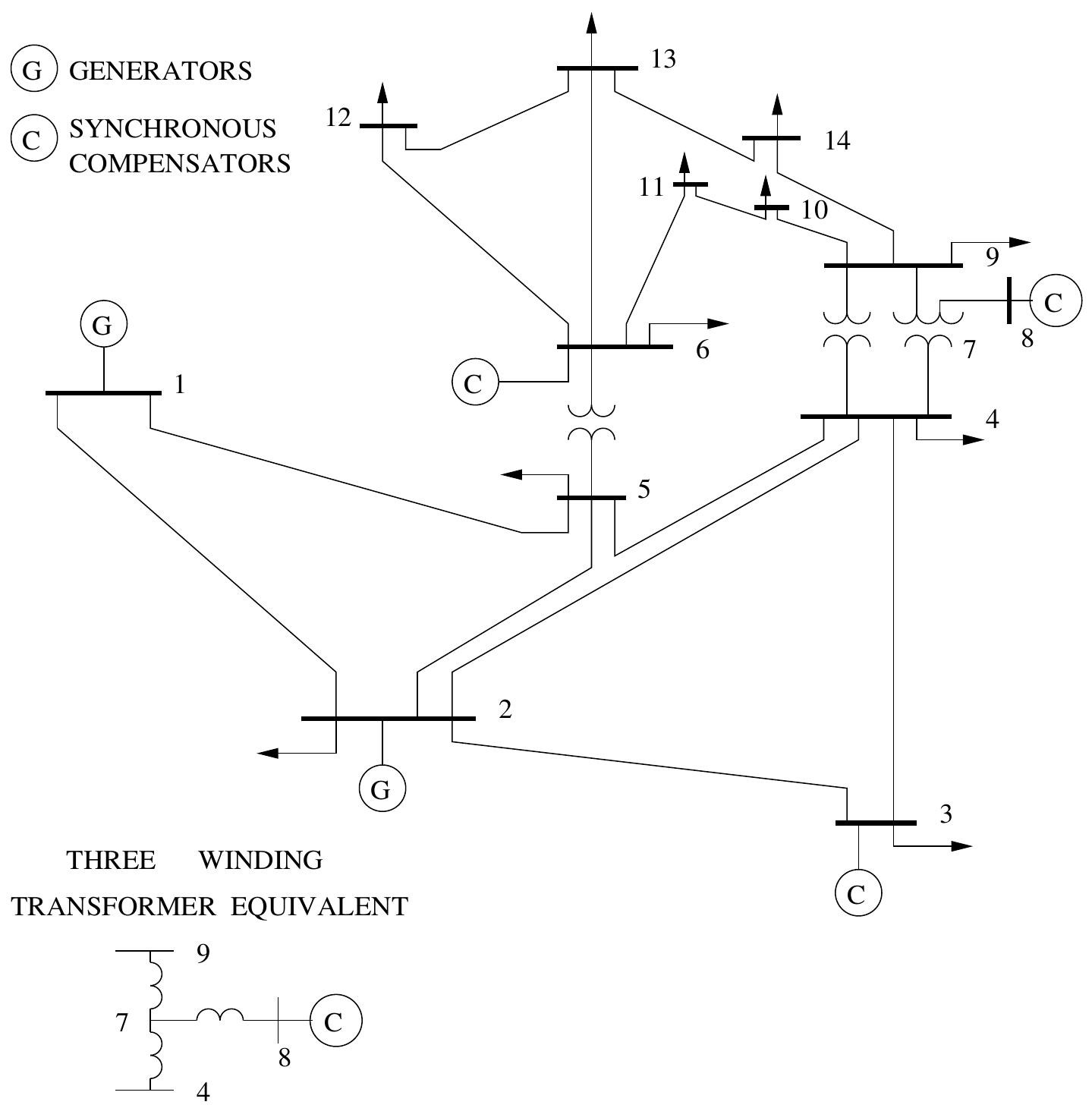
Figure 1: Technical representation of the IEEE 14-bus test system, extracted from [13]. It contains five synchronous machines of which two are generators. The one at bus 2 is taken as the slack bus for the modeling in this paper. Furthermore, there are 8 loads (buses 4, 5, 8, 9, 10, 11, 12, 13, and 14). Bus 7 is for the representation of the transformer.

The IEEE 14-bus system is a representation of a medium-voltage distribution grid. A graphical representation is in Figure 1, which is extracted from [13]. There are two generators, where the one at bus 2 is the slack bus, three synchronous compensators, and eight (complex) loads. Bus 7 is for the representation of the transformer only.

The generator at bus 1 and the synchronous compensators will be modeled with the swing equation, the slack bus 2 with the algebraic constraint introduced in Section III and the loads with the algebraic constraints for complex loads (see Section III also). The bus parameters haven been extracted from [13] and are presented in Table I. The resistance $R$ and reactance $X$ for the lines (taken from [13] as well) are summarized in Table II.

Having a description of the power grid in question enables us to have a look at the implementation in PowerDynamics.jl now.

TABLE I: Bus parameters of the IEEE 14-bus test system. INERTIA UNIT IS?

Bus	Type	$U\,[p.u.]$	$P\,[p.u.]$	$Q\,[p.u.]$	$D\,[p.u.]$	$H[p.u.\cdot s]$
1	Generator		2.32		2	5.148
2	Slack	1
3	Syn. Comp.		-0.942		2	6.54
4	Load		-0.478	0
5	Load		-0.076	-0.016
6	Syn. Comp.		-0.112		2	5.06
7	Load		0	0
8	Syn. Comp.		0		2	5.06
9	Load		-0.295	-0.166
10	Load		-0.09	-0.058
11	Load		-0.035	-0.018
12	Load		-0.061	-0.016
13	Load		-0.135	-0.058
14	Load		-0.149	-0.05

TABLE II: Line parameters of the IEEE 14-bus test system.

line number	from bus	to bus	$R\,[p.u.]$	$X\,[p.u.]$
1	1	2	0.01938	0.05917
2	1	5	0.05403	0.22304
3	2	3	0.04699	0.19797
4	2	4	0.05811	0.17632
5	2	5	0.05695	0.17388
6	3	4	0.06701	0.17103
7	4	5	0.01335	0.04211
8	4	7	0.0	0.20912
9	4	9	0.0	0.55618
10	5	6	0.0	0.25202
11	6	11	0.09498	0.1989
12	6	12	0.12291	0.25581
13	6	13	0.06615	0.13027
14	7	8	0.0	0.17615
15	7	9	0.0	0.11001
16	9	10	0.03181	0.0845
17	9	14	0.12711	0.27038
18	10	11	0.08205	0.19207
19	12	13	0.22092	0.19988
20	13	14	0.17093	0.34802

V Implementation in PowerDynamics.jl

In this section, we will show first how to implement the dynamics for the different buses presented in Section III in PowerDynamics.jl and then how create a power grid model from these bus dynamics definitions, in this case the IEEE 14-bus system.

V-A Defining the dynamics

The implementation of such a power grid in PowerDynamics.jl is strongly based on the $\mathtt{@DynamicNode}$ macro. A macro is a metaprogramming function that takes part of the source codes and modifies it at parsing time before giving it to the compiler, that creates the actual bitcode. In case of $\mathtt{@DynamicNode}$, this is used to hide all the complicated internals of PowerDynamics.jl and make the definition of a type of dynamics as easy as possible. The following examples are already provided by default in PowerDynamics.jl but using them as an example, any kind of dynamics can be implemented.

Using $\mathtt{@DynamicNode}$, the slack bus constraint from Section III is implemented as

⬇

1@DynamicNode SlackAlgebraic(U) <: OrdinaryNodeDynamicsWithMass(m_u=false) begin

2end [] begin

3 du = u - U

4end

where line breaks and line numbers have been added for easier orientation. The left part on the first line states the name of the new type $\mathtt{SlackAlgebraic}$ and the parameter name $\mathtt{U}$. Separated by the subtyping operator ($\mathtt{<:}$) comes the statement that it can be represented by an ordinary differential equation with a mass term, where the mass for the voltage m_u is set to $\mathtt{false}$, meaning $m^{u}=0$ from Section III as it is a constraint. The [] in line 2 states that there are no internal variables. And line 3 simply provides the formula for the dynamics and assigns it to $\mathtt{du}$. As m_u = false is given, this simply translates it to a constraint.

In a similar manner, the load is defined as an algebraic PQ-constraint

⬇

1@DynamicNode PQAlgebraic(S) <: OrdinaryNodeDynamicsWithMass(m_u=false) begin

2end [] begin

3 s = u*conj(i)

4 du = S - s

5end

In this case, an additional line was added to calculate the outflowing complex power $\mathtt{s}$ from the voltage $\mathtt{u}$ and the current $\mathtt{i}$ and then the definition of the constraint is written in line 4.

Concerning the generator and the synchronous compensators, we implemented the swing equation as

⬇

1@DynamicNode SwingEq(H, P, D, SOmega) <: OrdinaryNodeDynamics() begin

2 @assert D > 0 "damping (D) should be >0"

3 @assert H > 0 "inertia (H) should be >0"

4 SOmega_H = SOmega * 2pi / H

5end [[Somega, dSomega]] begin

6 p = real(u * conj(i))

7 du = u * im * Somega

8 dSomega = (P - D*Somega - p)*SOmega_H

9end

Again, the left part of the first line provides the name of the new type and the name of the parameters. Lines 2 to 4 are code that should be run only once. In this case these are consistency checks, that the damping and inertia are positive, and the reduction of the rated frequency $\mathtt{\Omega}$ and the inertia $\mathtt{H}$ to a single variable $\mathtt{\Omega\_H}$. In line 5, the variable name of the internal variable $\mathtt{\omega}$ and the name for its derivative $\mathtt{d\omega}$ are given. Finally, lines 6 to 8 implement Sections III and III by simply writing down the mathematical terms.

V-B Instantiating the power grid model

In order to create the grid model, we first have to instantiate the bus models simply by calling them with the corresponding parameter values from Table I, e.g.:

⬇

1SwingEq(H=5.148, P=2.32, D=2, SOmega=50) # for bus 1

2PQAlgebraic(S=-0.295-0.166im) # for bus 9

Within the actual code we simply loaded the data from a $\mathtt{.csv}$ file into and automatized this instantiation. The instantiated bus models should then be saved in an array called e.g. $\mathtt{nodes}$. Similarly, the admittance Laplacian should be generated from the line data in Table II and saved in a matrix called e.g. $\mathtt{LY}$. The actual grid model instatiation is then simply one line where the model is saved in the variable $\mathtt{g}$:

⬇

1g = GridDynamics(node_list, LY)

Now, $\mathtt{g}$ contains all the information of the power grid and in the following section we will show how to solve it.

VI Modeling Results

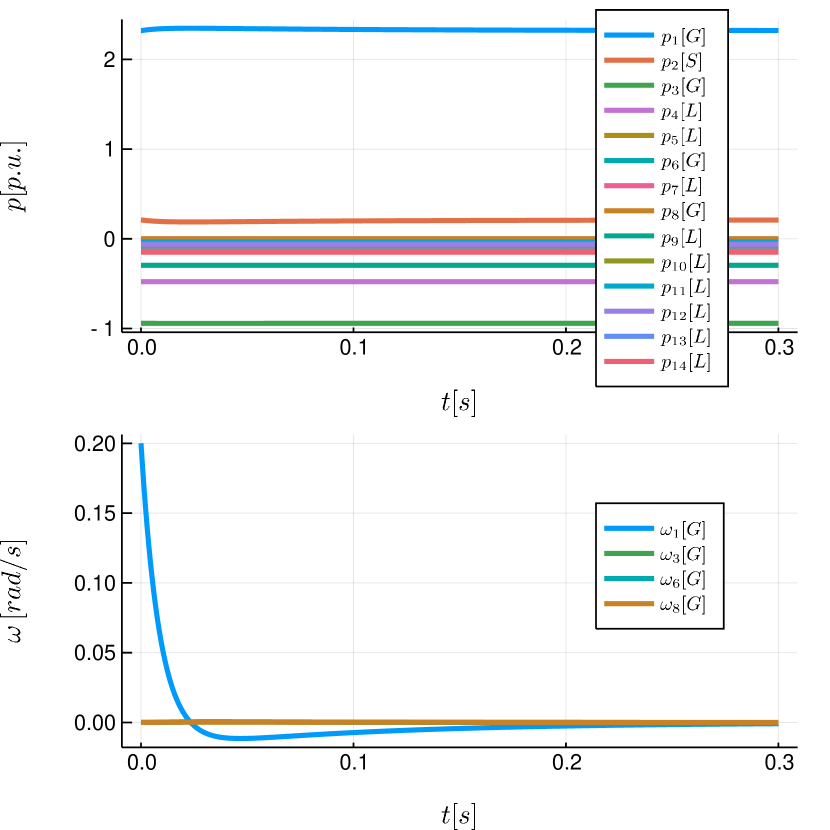
(a)

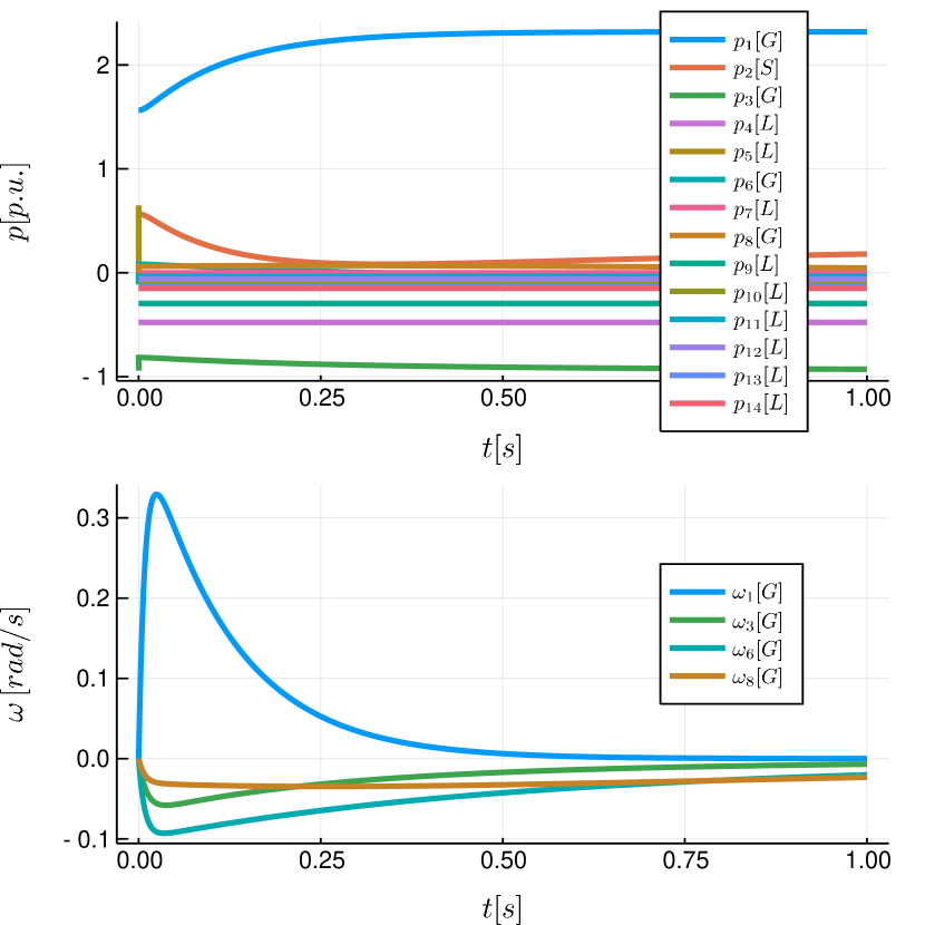
(b)

Figure 2: The two subfigures show the outflowing power (top) at each node and the angular frequency (bottom) for the buses modeled by the swing equation (1, 3, 6, 8) in for the two perturbation scenarios: (left) frequency perturbation at bus 1 and (right) line tripping of line 2 (between bus 1 and 5). The letter in bracets refers to the modeling type, i.e. $G$ for generator / synchronous compensator as swing equation, $S$ for the slack bus, and $L$ for a load as algebraic PQ-constraint.

Within this section, we will analyze two simple cases: (a) a frequency perturbation at the largest generator at bus 1 and (b) a line tripping event at of line 2 (between bus 1 and 5) (cmp. Figure 1).

Before we find the normal point of operation for the power grid, i.e. the fixed point of Sections III, III and III or synchronous state for the IEEE 14-bus system. For that, we use the grid model $\mathtt{g}$ generated in the previous Section V and use the function provided by PowerDynamics.jl:

⬇

1fp = operationpoint(g, ones(SystemSize(g)))

where $\mathtt{ones(SystemSize(g))}$ is a vector of the correct length for the initial condition of the fixed point search. $\mathtt{fp}$ is now a $\mathtt{State}$ object that we can use as initial condition for the solving the differential equations corresponding to the power grid.

VI-A Frequency perturbation

In order to model a frequency perturbation, one can simply take a copy of the fixed point as found before and adjust the initial frequency value:

⬇

1x0 = copy(fp)

2x0[1, :int, 1] += 0.2

The second line can be read as ‘‘add 0.2 to the 1${}^{\text{st}}$ internal variable of the 1${}^{\text{st}}$ node’’ which is the frequency $\omega$ as there is only one internal variable. Note that the first $\mathtt{1}$ refers to the node and then second $\mathtt{1}$ to the internal variable counter. The power grid with the initial condition $\mathtt{x0}$ can then be solved for a time span of 0.5 seconds by calling:

⬇

1sol = solve(g, x0, (0.0,.5))

The solution is shown in Figure 2a. It shows that the system is very stable against frequency perturbations. The actual dynamics is not so exciting as the system is very stable. Please note that this system was taken as an example to present on how easily one can model a power grid using PowerDynamics.jl, not to find new exciting dynamics.

VI-B Line tripping

To show some more dynamic behavior we simulated a line tripping as well. We model this effect by taking the operation point of the full power grid ($\mathtt{fp}$) as initial condition but defining a new admittance Laplacian where line 2 (between bus 1 and 5, see Tables II and 1) has been taken out (i.e. the admittance is set to $0$). Running the model with this new Laplacian yields Figure 2b.

In the frequency plot we identify how the frequency of bus 1, where the line tripping happened, compensates for the momentarily excess power at the bus. The lacking power in the rest of the grid is matched by the synchronous compensators whose frequency decreases in turn. Note that the angular frequency $\omega$ is shown, so with a division by $2\pi$ the maximal frequency deviation $f$ is $\approx 0.05\,$Hz. After about one second, the system recovers to the normal state of operation.

VII Conclusion & Outlook

Within this paper, we have seen how one one can use the Open-Source library PowerDynamics.jl in order to model the dynamics of a power grid with just a few lines of code. We have seen how the fundamental mathematical equations (given in Section III) translate to source code that reads exactly the same. We employed PowerDynamics.jl for the IEEE 14-bus distribution grid feeder in order to demonstrate how one can easily simulate faults and analyze the transient reaction of the power grid dynamics. As example scenarios we used a frequency perturbation and a line tripping.

Finally, this paper is really just a sneak preview with a simple example the publication of PowerDynamics.jl is planned for October 15, 2018. By then, we will have added more inverter control schemes and stochastic descriptions of intermittency due to renewable energy sources.

References

- [1] S. Auer, F. Hellmann, M. Krause, and J. Kurths, ‘‘Stability of synchrony against local intermittent fluctuations in tree-like power grids,’’ Chaos: An Interdisciplinary Journal of Nonlinear Science, vol. 27, no. 12, p. 127003, 2017.
- [2] S. Auer, ‘‘The stability and control of power grids with high renewable energy share,’’ Ph.D. dissertation, 2018.
- [3] B. Schäfer, C. Grabow, S. Auer, J. Kurths, D. Witthaut, and M. Timme, ‘‘Taming instabilities in power grid networks by decentralized control,’’ The European Physical Journal Special Topics, vol. 225, no. 3, pp. 569--582, 2016.
- [4] Siemens AG, ‘‘PSS® power system simulation and modeling software,’’ https://www.digsilent.de/en/powerfactory.html, accessed: 2018-08-28.
- [5] F. Milano, ‘‘PSAT,’’ http://faraday1.ucd.ie/psat.html, accessed: 2018-08-28.
- [6] F. Milano, L. Vanfretti, and J. C. Morataya, ‘‘An open source power system virtual laboratory: The psat case and experience,’’ IEEE Transactions on Education, vol. 51, no. 1, pp. 17--23, 2008.
- [7] J. Bezanson, A. Edelman, S. Karpinski, and V. B. Shah, ‘‘Julia: A fresh approach to numerical computing,’’ SIAM review, vol. 59, no. 1, pp. 65--98, 2017.
- [8] J. C. Richstein, ‘‘open energy modeling initiative,’’ http://www.openmod-initiative.org/, accessed: 2018-08-28.
- [9] JuliaLang, ‘‘The Julia Language,’’ https://julialang.org/, accessed: 2018-08-28.
- [10] A. C. Hindmarsh, P. N. Brown, K. E. Grant, S. L. Lee, R. Serban, D. E. Shumaker, and C. S. Woodward, ‘‘SUNDIALS: Suite of nonlinear and differential/algebraic equation solvers,’’ ACM Transactions on Mathematical Software (TOMS), vol. 31, no. 3, pp. 363--396, 2005.
- [11] P. W. Sauer and M. Pai, ‘‘Power system dynamics and stability,’’ Urbana, 1998.
- [12] P. Kundur, N. J. Balu, and M. G. Lauby, Power system stability and control. McGraw-hill New York, 1994, vol. 7.
- [13] S. K. M. Kodsi and C. A. Canizares, ‘‘Modeling and simulation of ieee 14 bus system with facts controllers,’’ Technical Report 2003-3, 2003.