Implicit Regularization in ReLU Networks with the Square Loss
Abstract
Understanding the implicit regularization (or implicit bias) of gradient descent has recently been a very active research area. However, the implicit regularization in nonlinear neural networks is still poorly understood, especially for regression losses such as the square loss. Perhaps surprisingly, we prove that even for a single ReLU neuron, it is impossible to characterize the implicit regularization with the square loss by any explicit function of the model parameters (although on the positive side, we show it can be characterized approximately). For one hidden-layer networks, we prove a similar result, where in general it is impossible to characterize implicit regularization properties in this manner, except for the “balancedness” property identified in Du et al. (2018). Our results suggest that a more general framework than the one considered so far may be needed to understand implicit regularization for nonlinear predictors, and provides some clues on what this framework should be.
1 Introduction
A major open question in the theory of deep learning is how neural networks generalize even when trained without any explicit regularization, and when there are far more learnable parameters than training examples. In such an underdetermined optimization problem, there are many global minima with zero training loss, and gradient descent seems to prefer solutions that generalize well (see Zhang et al. (2016)). Hence, it is believed that gradient descent induces an implicit regularization (or implicit bias) (Neyshabur et al., 2014, 2017), and characterizing this regularization/bias has been a subject for an extensive research in recent years.
The focus in the existing research is on finding a regularization function , where are the parameters of the model, such that if we apply gradient descent on the average loss, then it converges in some sense to a global optimum that minimizes . Thus, the function determines to which global optimum gradient descent converges. For example, it is known that for linear regression, gradient descent on the average square loss converges to the zero-loss solution with minimal norm (Zhang et al., 2016). For linear classification and exponentially-tailed losses (such as the logistic or exponential losses), gradient descent on linearly separable data converges in direction to the minimal norm predictor which attains a fixed positive margin over the data, also known as the max-margin solution (cf. Soudry et al. (2018)). Thus, in both cases is essentially the norm.
Once we move beyond simple linear classification and regression, the situation gets more complicated. This is especially so when considering the square loss (a setting which we focus on in this paper), where existing works still focus on predictors which express linear functions111See the related work section below for discussion of results on classification losses, which are relatively easier to tackle.. For example, there has been much effort to characterize the implicit regularization of gradient descent in matrix factorization. This problem corresponds to training a depth-2 linear neural network, and is considered a well-studied test-bed for studying implicit regularization in deep learning. Gunasekar et al. (2018c) conjectured that the implicit regularization in matrix factorization is the nuclear norm, and proved it for some restricted cases. This conjecture was further studied in a string of works (e.g., Belabbas (2020); Arora et al. (2019); Razin and Cohen (2020)) providing positive and negative evidence, and was formally refuted by Li et al. (2020). Focusing on a more specific setting, Woodworth et al. (2020) recently studied the implicit regularization in diagonal linear neural networks, namely, linear networks where the weight matrices have a diagonal structure. They find the regularization function and show how it interpolates between the and the norm depending on the initialization scale. This result was further generalized in Yun et al. (2020).
In this paper, we study implicit regularization with the square loss in nonlinear neural networks, when trained using gradient descent with infinitesimal step sizes (a.k.a. gradient flow). Perhaps surprisingly, we show that already for very simple such networks (involving a single ReLU neuron, or one thin hidden layer), the implicit regularization cannot be expressed by any explicit function of the model parameters. In other words, the model used to capture the implicit regularization in previous works cannot be used to capture the implicit regularization of nonlinear models in general (at least with respect to the square loss). However, on the positive side, we show that this implicit regularization can sometimes be captured by an explicit , but only up to some constant approximation factor. In a bit more detail, our contributions are as follows:
-
•
We start with single-neuron networks, namely, . If the activation function is strictly monotonic, then it is not hard to show that the implicit regularization is the norm. However, if is the ReLU function, then we show that the implicit regularization is not expressible by any nontrivial function of . A bit more precisely, suppose that is such that if gradient flow converges to a zero-loss solution , then is a zero-loss solution that minimizes . We show that such a function must be constant in . Hence, perhaps surprisingly, the approach of precisely specifying the implicit bias of gradient flow via a regularization function is not feasible in single-neuron networks.
-
•
On the positive side, we show that while the implicit bias of a ReLU neuron cannot be specified exactly by a regularization function, it can be expressed approximately, within a factor of , by the norm. That is, let be a zero-loss solution with a minimal norm, and assume that gradient flow converges to some point , then . Assuming is not too large, such a bound on the norm can be used to derive good statistical generalization guarantees, via standard techniques (cf. Shalev-Shwartz and Ben-David (2014)).
-
•
We extend our study to depth- ReLU networks. For such networks, an important implicit bias property shown in Du et al. (2018) is that gradient flow enforces the differences between square norms across different layers to remain invariant. Starting from a point close to zero, it implies that the magnitudes of all layers are automatically balanced. Thus, gradient flow induces a bias toward “balanced” layers. However, this bias is rather weak and is not related to properties that may allow us to obtain generalization guarantees, such as small norms, sparsity, or low rank. We consider networks with one hidden ReLU neuron, i.e., (where are the trained parameters), which is the simplest case of a depth- ReLU network. We show that the only bias which can be specified by a function of the model parameters is the balancedness property: Namely, is constant in the set of parameters that satisfy this property. Thus, no other implicit bias property can be expressed by such a function for single-hidden-neuron networks. This also has implications for general depth- ReLU networks: If is a function that specifies the implicit regularization of depth- networks, then in the special case of single-hidden-neuron networks, it does not induce bias except for enforcing the balancedness property. Hence, the implicit regularization function of depth- ReLU networks cannot be generally related to properties such as small norms or sparsity, which should apply also to single-hidden-neuron networks.
We again emphasize that since our results show the impossibility of characterizing the implicit regularization already for very simple networks, similar difficulties will be encountered in more general cases (such as ReLU networks of any depth and width).
Overall, our results suggest that the implicit regularization for ReLU networks with the square loss may not be expressible by an explicit function of the model parameters. On the positive side, they also suggest how this can be overcome by changing the model: Instead of looking for such an which captures the bias exactly, we might try to capture it approximately, as we did in the single ReLU neuron case. Another possible direction is to find a regularization function that is data-dependent in some simple way222Otherwise, a trivial solution is to define (where is the dataset) to be if are the parameters returned by gradient flow given , and otherwise., and does not depend just on the model parameters. We believe these are both interesting directions for further research.
Related Work
As we already discussed, implicit regularization in matrix factorization and linear neural networks was extensively studied, as a first step toward understanding implicit regularization in more complex models (see, e.g., Gunasekar et al. (2018c); Razin and Cohen (2020); Arora et al. (2019); Belabbas (2020); Eftekhari and Zygalakis (2020); Li et al. (2018); Ma et al. (2018); Woodworth et al. (2020); Gidel et al. (2019); Li et al. (2020); Yun et al. (2020)). In Razin and Cohen (2020) it was shown that gradient flow in matrix factorization may approach a global minimum at infinity rather than converging to a global minimum with a finite norm. This result suggests that the implicit regularization in matrix factorization may not be expressible by norms. The main conceptual differences from our paper are that we rule out all regularization functions, and that our result holds already if we assume that gradient flow converges to some global minimum with a finite norm.
Oymak and Soltanolkotabi (2019) studied the implicit bias of gradient descent in certain nonlinear models. They showed that under some assumptions, gradient descent is guarranteed to converge to a zero-loss solution with a bounded norm. Their results have implications on the implicit regularization of single-neuron networks with a strictly monotonic activation function, which we discuss in Remark 3.1. Williams et al. (2019) and Jin and Montúfar (2020) studied the dynamics and implicit bias of gradient descent in wide depth- ReLU networks with input dimension .
The conceptually closest works to ours are Dauber et al. (2020); Suggala et al. (2018), which show that variants of gradient descent on some (specially crafted) convex optimization problems do not converge to a closest Euclidean solution, or cannot be explained by any reasonable implicit regularization function. These works, as well as ours, consider the limitations of implicit regularization, but our results apply to a standard learning problem, namely, learning neural networks. Thus, while the results of Dauber et al. (2020); Suggala et al. (2018) demonstrate that there are learning problems that cannot be explained by any reasonable regularization function, we show that this phenomenon occurs already for simple ReLU networks.
The implicit bias of gradient descent in classification tasks is also widely studied. Soudry et al. (2018) showed that gradient descent on linearly-separable binary classification problem with an exponentially-tailed loss (e.g., the exponential loss and the logistic loss), converges to the maximum margin direction. This analysis was extended to other loss functions, tighter convergence rates, nonseparable data, and variants of gradient-based optimization algorithms (Nacson et al., 2019; Ji and Telgarsky, 2018b; Ji et al., 2020; Gunasekar et al., 2018a; Shamir, 2020). The problem was also studied for more complex models, such as linear neural networks (Gunasekar et al., 2018b; Ji and Telgarsky, 2018a; Moroshko et al., 2020; Yun et al., 2020), and neural networks with homogeneous activation functions (Lyu and Li, 2019; Chizat and Bach, 2020; Xu et al., 2018).
2 Preliminaries
Notations. We use bold-faced letters to denote vectors, e.g., . For we denote by the Euclidean norm.
Single-neuron networks. Let be a training dataset, where for every we have and . We consider empirical-loss minimization of a single-neuron network, with respect to the square loss. Thus, the objective is given by
| (1) |
where is a nonlinear activation function. Let denote the data matrix, i.e., the rows of are , and let . We have
where is applied component-wise. We assume that the data is realizable, that is, . Moreover, we focus on settings where the network is overparameterized, in the sense that has multiple (or even infinitely many) global minima.
We analyze the implicit regularization of gradient flow on the objective given by Eq. 1. This setting captures the behaviour of gradient descent with infinitesimally small step size. Let be the trajectory of gradient flow, where is the initial point. The dynamics of is given by the differential equation
If exists then we denote it by . We note that gradient flow is not guaranteed to converge to a global minimum (cf. Yehudai and Shamir (2020)). In the overparameterized setting there can be infinitely many global minima, and we study to which one gradient flow converges, assuming that it converges to a global minimum.
3 Warm up – strictly monotonic activation functions
We first analyze the implicit regularization of gradient flow on the objective given by Eq. 1, where the activation function is strictly monotonic. In this case, we show that the implicit bias is simply the norm: Namely, the point closest to on which .
Theorem 3.1.
Consider gradient flow on the objective given by Eq. 1, where is a strictly monotonic activation function. If exists and , then .
Proof.
Since is strictly monotonic, then for every we have iff . The KKT optimality conditions for the problem
are
Note that since the constraints are affine functions, then the conditions are both necessary and sufficient.
The second condition holds in since . Moreover, we have
Thus, is always spanned by , and hence the first condition also holds. ∎
Remark 3.1.
By Oymak and Soltanolkotabi (2019), if is continuously differentiable and there are positive constants such that for every , then is guaranteed to converge to a global optimum that is closest to . In Theorem 3.1, our assumption on is weaker, but we assume that exists and (which is a common assumption when considering implicit regularization).
4 The implicit regularization of a ReLU neuron is not expressible by
In this section we study the implicit regularization of gradient flow on the objective given by Eq. 1, where and is the ReLU function. We impose the convention that even though the ReLU function is not differentiable at , we take . This convention is required for analyzing gradient flow with , since if then would stay at indefinitely. For simplicty, in our proofs we assume that , but our results hold for every positive value.
Assume that the implicit regularization can be expressed as a function , namely, if gradient-flow converges to a global minimum , then we have . We will first show that unlike the case of strictly monotonic activations, the implicit bias of is not the norm, and in fact, data-dependent in a nontrivial way. Then, we will extend this result, and show that is trivial, namely, constant in . Thus, the behavior of has a complicated data-dependent behavior, and cannot be written down as minimizing some function dependent only on , among all zero-loss solutions.
4.1 is not the norm
We show that the implicit regularization of a single ReLU neuron is not the norm. Thus, the implicit regularization of ReLU is different than that of strictly monotonic activation functions considered in Section 3. Specifically, in the following theorem we analyze the behavior of gradient flow for some family of inputs. The theorem considers a datasets of the form , where is a parameter. We show that gradient flow starting from with the input , converges to a zero-loss solution which is not a minimal-norm zero-loss solution, and that the parameter controls the ratio between and the minimal-norm of a zero-loss solution. Hence, the implicit regularization is not the norm. We will also use this theorem later in order to show additional results.
Theorem 4.1.
Let , and let
Let and let . Consider gradient flow with input , starting from , on the objective given by Eq. 1, where is the ReLU function. Let . Note that for every we have , and thus . Moreover, note that the global optimum with the minimal norm is . We have:
-
•
If then .
-
•
If then for some independent of .
-
•
If then for some independent of .
-
•
If then for some independent of .
Proof sketch (for complete proof see Appendix A).
The trajectory is the solution of the initial value problem defined by the differential equation
| (2) |
and the initial condition . Here, are the rows of the matrix , and are the components of .
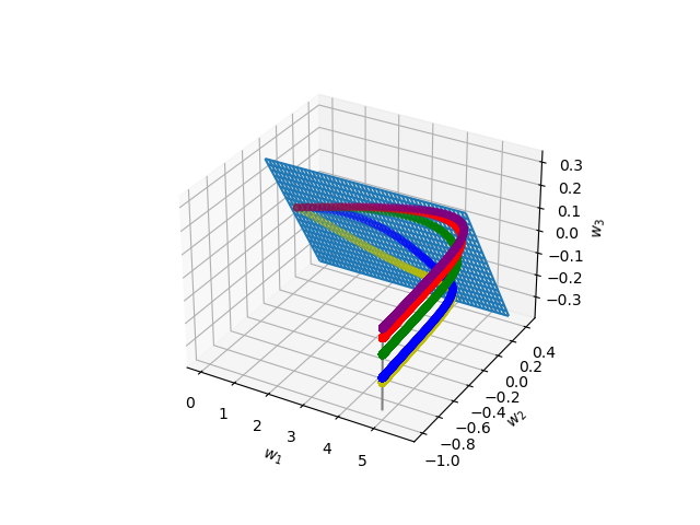
In Figure 1, we show the trajectories of gradient descent (an empirical simulation), for and . The grey line denotes the set , and the hyperplane corresponds to (where ). Note that the trajectories for consist of two parts. In the first part , and in the second part . We note that in the second part, the component remains constant. Indeed, by Eq. 2, the change in is spanned by , and if then it is spanned only by (note that if then ). Since have as their third component, then does not change. Intuitively, the parameter controls the extent to which decreases during the first part, before reaching the second part in which it stays constant. In the proof we analyze these trajectories formally.
For , we show that the solution to Eq. 2 is , where is given by
Here, is obtained from by omitting the third column and third row, , and denotes the matrix exponential. Note that . Moreover, note that in order to show that this trajectory satisfies Eq. 2, it suffices to show that for every and , and that satisfies the linear differential equation obtained form Eq. 2 by plugging in and .
For , we show that the solution to Eq. 2 consists of two parts: The first part is where for some , and second part is where . In the first part, we have
and for every and . Then, in the second part, remains constant, and is given by
Here, is obtained from by omitting the third column and third row. Note that . In this part, we have for and .
In the proof, we show for both parts, that the trajectories satisfy Eq. 2. Moreover, we investigate the value of in order to obtain the required bounds for each . ∎
4.2 is trivial
We now prove the following theorem, which implies that is trivial and does not induce an implicit bias.
Theorem 4.2.
Consider gradient flow starting from , on the objective given by Eq. 1, where is the ReLU function. Let , such that for every input where gradient flow converges to with , we have . Then, is constant in .
Let and . Let be the rows of . Suppose that given input , gradient flow with converges to . Note that by rotating , the trajectory is rotated accordingly
Thus, for every rotation matrix , given input gradient flow converges to .
Let . By Theorem 4.1, all points in are global minima for all inputs , but gradient-flow converges to different points , depending on . Hence, we have . Thus, Theorem 4.1 implies that . We use this property in order to prove Theorem 4.2.
Let . We denote . By changing the input in Theorem 4.1 to , we deduce that . Indeed, all points in are global minima for all inputs , but gradient-flow converges to different points , depending on . Let be such that . For every with , and such that and , by choosing an appropriate rotation we obtain . Finally, as we show in the following lemma, this property implies that is constant over , and thus we complete the proof of Theorem 4.2.
Lemma 4.1.
Let be constants. Let , and let be a function such that for every , vector with , and vector such that and , we have . Then, for every .
Proof sketch (for complete proof see Appendix B).
First, we show that is radial, namely, there exists a function such that for every . Assume that are such that for some , and is sufficiently small. We show that there exists such that for some with and . By our assumption on , it implies that , and hence is radial.
Thus, it suffices to show that for every . Using our assumption on , we show that for every we have . The assumption on also implies that , and that for a sufficiently large . Therefore, we have , and hence as required. ∎
Remark 4.2 ( is trivial also for ).
5 The implicit regularization of a ReLU neuron is approximately the norm
While the implicit regularization of ReLU neuron cannot be expressed as a function , in this section we show that it can be expressed approximately, within a factor of , by the norm. This implies that even without early stopping, if the data can be labeled by a ReLU neuron with small norm, then gradient flow will converge to a ReLU neuron whose norm is not much larger. Since a ReLU neuron is just a linear function composed with a fixed nonlinearity, this can be used to derive good statistical generalization guarantees, via standard techniques (cf. Shalev-Shwartz and Ben-David (2014)).
Theorem 5.1.
Consider gradient flow on the objective given by Eq. 1, where is a monotonically non-decreasing activation function (e.g., ReLU). Assume that exists and . Let . Then, .
Proof.
First, note that
Since is monotonically non-decreasing then
and . Hence,
Therefore, we have
Thus, .
Hence,
∎
Remark 5.1.
Note that Theorem 5.1 implies that if then . By Theorem 4.2, the implicit regularization cannot be expressed as a function of . Hence, while the implicit regularization of a ReLU neuron cannot be expressed exactly as a function of , it can be expressed approximately, within a factor of , by the norm.
6 Depth- ReLU networks
In Section 4, we showed that the implicit regularization of a single ReLU neuron is not expressible by any nontrivial function of . In this section we will show an analogous result for networks with one hidden ReLU neuron (namely, ), which is the simplest case of a depth- ReLU network. Since our focus here is on impossibility results, then our results for this simple case imply impossibility results also for more general cases.
By Du et al. (2018), in feed-forward ReLU networks, gradient flow enforces the differences between square norms across different layers to remain invariant. Thus, if gradient flow starts from a point close to , then the magnitudes of all layers are automatically balanced. In the case of single-hidden-neuron networks, it implies that (the norm of the weights vector of the first layer) is roughly equal to (the weight in the second layer). Hence, gradient flow induce a bias toward balanced layers. However, this bias is considered weak and does not allow us to derive generalization guarantees. Hence, there has been much effort to characterize the implicit regularization and to understand whether it is related to properties such as small norms, sparsity, or low ranks (cf. Gunasekar et al. (2018c); Razin and Cohen (2020); Arora et al. (2019); Woodworth et al. (2020); Belabbas (2020); Li et al. (2020)). We show that in single-hidden-neuron networks, the only bias which can be specified by a regularization function (where are the network parameters) is the balancedness property described above. Namely, is constant in the set of parameters that satisfy the balacedness property.
Recall that in our study of single-neuron networks in Section 4, we first analyzed the behavior of gradient flow for some specific inputs (Theorem 4.1), and then used this result in order to show that the implicit regularization function is trivial (Theorem 4.2). Here, we proceed in a similar manner, but the first part is based on empirical results rather than on a theoretical proof. Thus, we first run gradient descent for some specific inputs, and observe empirically that it converges to points that clearly satisfy a certain technical property. Then, making the explicit assumption that the technical property holds, we prove that the regularization function is constant in the set of parameters that satisfy the balacedness property.
We now proceed to the formal results. Let , and consider the neural network , where is the ReLU function. Let be a training dataset, and let be the corresponding data matrix. We analyze the implicit regularization of gradient flow on the objective
| (3) |
We assume that the data is realizable, i.e., . The run of gradient flow starts from , where , and is a small number333Note that if we start from then gradient flow stays at this point indefinitely, since the gradient there is . This is avoided by making either the scalar or the vector non-zero, and we focus on the former as it makes the analysis cleaner.. Let be the trajectory of gradient flow where for some , and let (assuming that the limit exists). In addition, we define the limit point of gradient flow (on inputs ) as , assuming the limit exists. This follows a standard practice in analyzing the implicit regularization of gradient flow, where we consider the flow’s limit assuming it starts infinitesimally close to (see, e.g., Gunasekar et al. (2018c); Razin and Cohen (2020); Arora et al. (2019); Woodworth et al. (2020); Li et al. (2020)).
We are interested in understanding the properties of any possible implicit regularization function : Namely, a function that for every input to gradient flow, if exists and , then we have . Whereas for a single ReLU neuron, we showed that is necessarily constant, the situation for a single hidden-neuron is more complex, because gradient flow is already known to induce the following nontrivial balacedness property444Du et al. (2018) showed the lemma for the more general case of fully-connected networks with homogeneous activation functions. See Appendix C.1 for a simpler proof for our setting.:
Lemma 6.1 (Du et al. (2018)).
Let be the trajectory of gradient flow on Eq. 3, starting from some . Then
As a consequence, we have the following corollary.
Corollary 6.1.
Let and let . For every we have .
By Corollary 6.1, we have , and hence . As a result, not all parameters can be reached by gradient flow – only those which satisfy the “balancedness” property above. However, this property in itself is rather weak, and does not necessarily induce bias towards properties which may aid in generalization, such as small norms or sparsity. Is there any stronger implicit regularization at play here? To answer that, it is natural to consider the behavior of the implicit regularization function on the set of “balanced” parameters. In what follows, we will argue that is constant on . Thus, may induce a bias toward , namely, enforce the “balancedness” of and , but it does not induce any additional bias within .
In order to show that is constant in , we start with an empirical study of gradient descent for some specific inputs. Then, under a mild assumption based on the empirical results, we prove that is constant.
6.1 Empirical results
In Theorem 4.1 we showed that the implicit regularization of a single ReLU neuron is not the norm. We now demonstrate an analogous behavior in single-hidden-neuron networks.
Let be the matrix from Theorem 4.1. Let be the vector from Theorem 4.1 with , i.e., . Let . Note that for every and we have . By Theorem 4.1, for different values of , gradient flow on a single neuron with the input converges to different points in a set of global minima. We now show empirically that a similar behavior appears also in single-hidden-neuron networks: For different values of , gradient descent with the input , starting from for a fixed , converges to different points with . We denote .
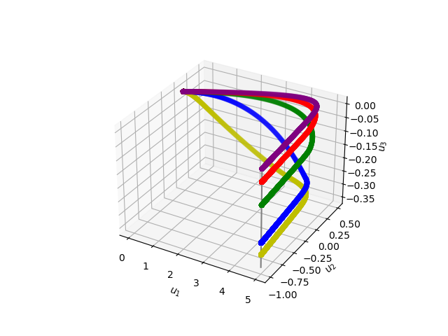
In Figure 2(a), we show the trajectories of gradient descent starting from , for . The grey line denotes the set . We note that while the trajectories in Figure 2(a) have similar shapes to the trajectories shown in Figure 1 for the case of a single-neuron network, they are not identical. Indeed, the dynamics of the problems are different. This experiment demonstrates that for and different values of , gradient descent converges to different points .
Since we are interested in gradient flow starting from for , we need to consider where . Consider , and let and . We now show empirical evidence that strongly supports the following assumption, which will be the key used to prove that the implicit regularization function is constant as discussed earlier:
Assumption 6.1.
For every sufficiently small , gradient flow starting from on the inputs and , converges to zero loss. Moreover, exists and is negative.
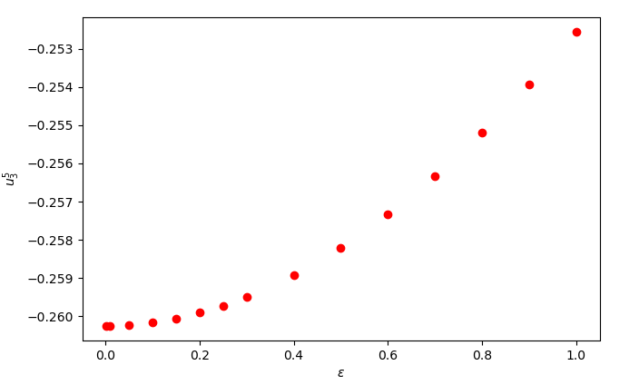
We turn to present this empirical evidence. Since we are interested in simulating gradient flow, we used gradient descent with a small learning rate of . We ran gradient descent starting from , for and . In all cases we reached loss smaller than , which suggests that the first part of the assumption holds. We now turn to the second part of the assumption. In Figure 2(b) we show for different values of , the value of in the last iteration of gradient descent starting from and reaching loss smaller than . This experiment suggests that exists and is negative.
Finally, we show that Assumption 6.1 easily implies the following corollary:
Corollary 6.2.
Under Assumption 6.1, for the inputs and , the limit points of gradient flow are and (respectively), such that and for some .
Proof.
First, since by Assumption 6.1 for every sufficiently small the loss converges to zero, then for every sufficiently small we have , and hence we also have . Clearly, for every we have , since if then the third component of is for every . Therefore, . Finally, by Assumption 6.1, exists and is negative. Overall, we have for some , and . ∎
6.2 is constant in the set of balanced parameters
We now show that the regularization function is constant in the set of balanced parameters. Since the limit point of gradient flow is in , then it is uniquely determined by the point , and hence, intuitively, we can think about as a point in . More formally, let be such that for , and . Note that for every we have , and that is bijective. Let be such that .
We state our main theorem on single-hidden-neuron networks:
Theorem 6.2.
Under Assumption 6.1, the function is constant in . Therefore, is constant in .
Intuitively, the theorem follows from the following argument. By Corollary 6.2, for the input , gradient flow converges to such that , even though every corresponds to a zero-loss solution. Hence, gradient flow prefers over all other points in . Similarly, for the input gradient flow converges to such that for some , even though every corresponds to a zero-loss solution. Hence, it prefers over all other points in . It implies that . Then, by rotating and scaling the inputs to gradient flow, and by using Lemma 4.1, we show that is constant in .
To prove the theorem more formally, we start with some additional notations. For an input to gradient flow, we denote , namely, the vectors in that correspond to global minima of . Let and let . Note that iff iff . Therefore, we have . Let , namely, the vector that corresponds to the limit point. Since , then . Indeed, we have
and since .
Note that by Corollary 6.2, for the inputs and , the limit points of gradient flow are and (respectively), such that and , and therefore we have the following. Let . We have , and . Moreover, since for every we have , then , and therefore for every we have . Since and , then we have .
We now utilize the following lemma, which considers the effect on the limit point of rotating and scaling the input to gradient flow. The lemma follows by analyzing the trajectories of gradient flow with the modified inputs. See Appendix C.2 for a proof.
Lemma 6.2.
Let be an input to gradient flow, let be its limit point, and let .
-
1.
Let be a rotation matrix. The limit point of gradient flow with input is . Thus, .
-
2.
Let . The limit point of gradient flow with input is . Thus, .
By rotating and scaling the inputs from Corollary 6.2, and using Lemma 6.2, we obtain the following corollary (see Appendix C.3 for a formal proof).
Corollary 6.3.
Under Assumption 6.1, there is a vector and a constant , such that for every and with , and for every such that and , we have .
Acknowledgements
This research is supported in part by European Research Council (ERC) grant 754705.
References
- Arora et al. [2019] S. Arora, N. Cohen, W. Hu, and Y. Luo. Implicit regularization in deep matrix factorization. In Advances in Neural Information Processing Systems, pages 7413–7424, 2019.
- Belabbas [2020] M. A. Belabbas. On implicit regularization: Morse functions and applications to matrix factorization. arXiv preprint arXiv:2001.04264, 2020.
- Chizat and Bach [2020] L. Chizat and F. Bach. Implicit bias of gradient descent for wide two-layer neural networks trained with the logistic loss. arXiv preprint arXiv:2002.04486, 2020.
- Dauber et al. [2020] A. Dauber, M. Feder, T. Koren, and R. Livni. Can implicit bias explain generalization? stochastic convex optimization as a case study. arXiv preprint arXiv:2003.06152, 2020.
- Du et al. [2018] S. S. Du, W. Hu, and J. D. Lee. Algorithmic regularization in learning deep homogeneous models: Layers are automatically balanced. In Advances in Neural Information Processing Systems, pages 384–395, 2018.
- Eftekhari and Zygalakis [2020] A. Eftekhari and K. Zygalakis. Implicit regularization in matrix sensing: A geometric view leads to stronger results. arXiv preprint arXiv:2008.12091, 2020.
- Gidel et al. [2019] G. Gidel, F. Bach, and S. Lacoste-Julien. Implicit regularization of discrete gradient dynamics in linear neural networks. In Advances in Neural Information Processing Systems, pages 3202–3211, 2019.
- Gunasekar et al. [2018a] S. Gunasekar, J. Lee, D. Soudry, and N. Srebro. Characterizing implicit bias in terms of optimization geometry. arXiv preprint arXiv:1802.08246, 2018a.
- Gunasekar et al. [2018b] S. Gunasekar, J. D. Lee, D. Soudry, and N. Srebro. Implicit bias of gradient descent on linear convolutional networks. In Advances in Neural Information Processing Systems, pages 9461–9471, 2018b.
- Gunasekar et al. [2018c] S. Gunasekar, B. Woodworth, S. Bhojanapalli, B. Neyshabur, and N. Srebro. Implicit regularization in matrix factorization. In 2018 Information Theory and Applications Workshop (ITA), pages 1–10. IEEE, 2018c.
- Ji and Telgarsky [2018a] Z. Ji and M. Telgarsky. Gradient descent aligns the layers of deep linear networks. arXiv preprint arXiv:1810.02032, 2018a.
- Ji and Telgarsky [2018b] Z. Ji and M. Telgarsky. Risk and parameter convergence of logistic regression. arXiv preprint arXiv:1803.07300, 2018b.
- Ji et al. [2020] Z. Ji, M. Dudík, R. E. Schapire, and M. Telgarsky. Gradient descent follows the regularization path for general losses. In Conference on Learning Theory, pages 2109–2136. PMLR, 2020.
- Jin and Montúfar [2020] H. Jin and G. Montúfar. Implicit bias of gradient descent for mean squared error regression with wide neural networks. 2020.
- Li et al. [2018] Y. Li, T. Ma, and H. Zhang. Algorithmic regularization in over-parameterized matrix sensing and neural networks with quadratic activations. In Conference On Learning Theory, pages 2–47. PMLR, 2018.
- Li et al. [2020] Z. Li, Y. Luo, and K. Lyu. Towards resolving the implicit bias of gradient descent for matrix factorization: Greedy low-rank learning. arXiv preprint arXiv:2012.09839, 2020.
- Lyu and Li [2019] K. Lyu and J. Li. Gradient descent maximizes the margin of homogeneous neural networks. arXiv preprint arXiv:1906.05890, 2019.
- Ma et al. [2018] C. Ma, K. Wang, Y. Chi, and Y. Chen. Implicit regularization in nonconvex statistical estimation: Gradient descent converges linearly for phase retrieval and matrix completion. In International Conference on Machine Learning, pages 3345–3354. PMLR, 2018.
- Moroshko et al. [2020] E. Moroshko, B. E. Woodworth, S. Gunasekar, J. D. Lee, N. Srebro, and D. Soudry. Implicit bias in deep linear classification: Initialization scale vs training accuracy. Advances in Neural Information Processing Systems, 33, 2020.
- Nacson et al. [2019] M. S. Nacson, J. Lee, S. Gunasekar, P. H. P. Savarese, N. Srebro, and D. Soudry. Convergence of gradient descent on separable data. In The 22nd International Conference on Artificial Intelligence and Statistics, pages 3420–3428. PMLR, 2019.
- Neyshabur et al. [2014] B. Neyshabur, R. Tomioka, and N. Srebro. In search of the real inductive bias: On the role of implicit regularization in deep learning. arXiv preprint arXiv:1412.6614, 2014.
- Neyshabur et al. [2017] B. Neyshabur, S. Bhojanapalli, D. McAllester, and N. Srebro. Exploring generalization in deep learning. In Advances in Neural Information Processing Systems, pages 5947–5956, 2017.
- Oymak and Soltanolkotabi [2019] S. Oymak and M. Soltanolkotabi. Overparameterized nonlinear learning: Gradient descent takes the shortest path? In International Conference on Machine Learning, pages 4951–4960, 2019.
- Razin and Cohen [2020] N. Razin and N. Cohen. Implicit regularization in deep learning may not be explainable by norms. arXiv preprint arXiv:2005.06398, 2020.
- Shalev-Shwartz and Ben-David [2014] S. Shalev-Shwartz and S. Ben-David. Understanding machine learning: From theory to algorithms. Cambridge university press, 2014.
- Shamir [2020] O. Shamir. Gradient methods never overfit on separable data. arXiv preprint arXiv:2007.00028, 2020.
- Soudry et al. [2018] D. Soudry, E. Hoffer, M. S. Nacson, S. Gunasekar, and N. Srebro. The implicit bias of gradient descent on separable data. The Journal of Machine Learning Research, 19(1):2822–2878, 2018.
- Suggala et al. [2018] A. Suggala, A. Prasad, and P. K. Ravikumar. Connecting optimization and regularization paths. Advances in Neural Information Processing Systems, 31:10608–10619, 2018.
- Williams et al. [2019] F. Williams, M. Trager, D. Panozzo, C. Silva, D. Zorin, and J. Bruna. Gradient dynamics of shallow univariate relu networks. In Advances in Neural Information Processing Systems, pages 8378–8387, 2019.
- Woodworth et al. [2020] B. Woodworth, S. Gunasekar, J. D. Lee, E. Moroshko, P. Savarese, I. Golan, D. Soudry, and N. Srebro. Kernel and rich regimes in overparametrized models. arXiv preprint arXiv:2002.09277, 2020.
- Xu et al. [2018] T. Xu, Y. Zhou, K. Ji, and Y. Liang. When will gradient methods converge to max-margin classifier under relu models? arXiv preprint arXiv:1806.04339, 2018.
- Yehudai and Shamir [2020] G. Yehudai and O. Shamir. Learning a single neuron with gradient methods. arXiv preprint arXiv:2001.05205, 2020.
- Yun et al. [2020] C. Yun, S. Krishnan, and H. Mobahi. A unifying view on implicit bias in training linear neural networks. arXiv preprint arXiv:2010.02501, 2020.
- Zhang et al. [2016] C. Zhang, S. Bengio, M. Hardt, B. Recht, and O. Vinyals. Understanding deep learning requires rethinking generalization. arXiv preprint arXiv:1611.03530, 2016.
Appendix A Proof of Theorem 4.1
Lemma A.1.
Let be an invertible matrix, and let . Consider the dynamics of given by the differential equation
Then, we have
| (4) |
where denotes the matrix exponential.
A.1 Proof for
The trajectory obeys the dynamics
where the last equality is since . Hence, since we also have , then is spanned by . Note that the third components in are , and therefore the third component in is for all . For a vector , we denote . We also denote by the matrix whose rows are and . Note that for we have . Thus, we have
| (5) |
If for then the above equals
By Lemma A.1, the solution to the above equation is
| (6) |
Let . We will show that the trajectory from Eq. 6 satisfies for every . Therefore, it satisfies Eq. 5 for every . It implies that , and therefore as required.
Lemma A.2.
The trajectory from Eq. 6 satisfies for every .
Proof.
By straightforward calculations we obtain
Moreover, we have
Since , then the above is at least
∎
A.2 Proof for
We show that the trajectory consists of two parts. In the first part, where for some , we have for every . Then, for , we have , , and .
A.2.1 Part 1
Recall that the trajectory obeys the dynamics
| (7) |
If for every then the above equals
By Lemma A.1, the solution to the above equation is
| (8) |
Let . We will show that the trajectory from Eq. 8 satisfies for every for some . Therefore, it satisfies Eq. 7 for . Hence, gradient flow follows the trajectory from Eq. 8 where . We will also investigate the values of the components of , since it is the starting point of the second part of the trajectory.
Note that for every we have , and therefore . Since we also have , then Eq. 8 implies
Let be the eigenvalues of , let , and let such that . Thus, we have
| (9) |
where .
Lemma A.3.
Let be the trajectory from Eq. 9. For every , there exists , such that for every , , and for some (independent of ), where and satisfies the following:
-
•
If then .
-
•
If then .
-
•
If then .
A.2.2 Part 2
In Lemma A.3 we established the trajectory for . We need to find the trajectory that satisfies the dynamics in Eq. 7 for , with the initial value obtained in Lemma A.3 .
Let . Consider the dynamics from Eq. 7, where . Since and , and since for , then we have
We will find the trajectory that satisfies
| (10) |
with the initial value , and show that for every . Such a trajectory obeys the dynamics in Eq. 7 for , with the initial value , as required.
For a vector , we denote . We also denote by the matrix whose rows are and . Since both and have as their third components, then satisfies Eq. 10 iff the third component satisfies
| (11) |
and the first two components satisfy
| (12) |
Consider the trajectory for , such that the first two components follow the trajectory from the above equation, and the third component is constant, i.e., for all . Note that this trajectory satisfies Eq. 11 and Eq. 12, and hence satisfies Eq. 10. It also satisfies the initial condition . Thus, it remains to show that for every . Since by Eq.A.2.2 we have , then we have . By Lemma A.3, it follows that is in the required interval, and thus it completes the proof of the theorem.
From the following two lemmas it follows that for all .
Lemma A.4.
For every and , we have .
Proof.
Since and have in their third components, then it suffices to show that for every and . By Lemma A.3, we have , where and .
For every , by straightforward calculations we obtain
Since and , the above is at least
Next, we have
∎
Lemma A.5.
For every , we have .
Proof.
By Lemma A.3, we have , where and . The first two components in are , and the third component is . Hence, in order to show that
it suffices to show that .
We have
| (15) |
Note that the above equals to
Since , then the above expression is monotonically descreasing w.r.t. . Also, since , then by plugging in to Eq. A.2.2 we obtain
Let denote the r.h.s. of the above inequality. Note that . Hence, in order to show that for every , it suffices to show that for all .
We denote
Thus, . Since , it is easy to verify that and . Thus,
We have
Since then the above is at most
∎
A.2.3 Proof of Lemma A.3 for
Here, we have , , and . The proof of Lemma A.3 for follows from the following lemmas.
Lemma A.6.
Let be the trajectory from Eq. 9. For , we have for every .
Proof.
By straightforward calculations, we obtain
Moreover, we have
Since , then the above is at least
∎
Lemma A.7.
Let be the trajectory from Eq. 9. There exists such that and for every we have .
Proof.
We have
Let
Note that . Thus, iff , and iff . We will show that there exists such that and for every we have .
Consider the derivative of
We have iff
Note that this equation has a single solution. Since , it follows that has at most one additional root. It is easy to verify that and . Hence, iff for some , and for every . ∎
Lemma A.8.
Proof.
We have
We also have
∎
Lemma A.9.
A.2.4 Proof of Lemma A.3 for
Here, we have , , and . The proof of Lemma A.3 for follows from the following lemmas.
Lemma A.10.
Let be the trajectory from Eq. 9. For , we have for every .
Proof.
By straightforward calculations, we obtain
Moreover, we have
Since , then the above is at least
∎
Lemma A.11.
Let be the trajectory from Eq. 9. There exists such that , and for every we have .
Proof.
We have
Let
Note that . Thus, iff , and iff . We will show that there exists such that and for every we have .
Consider the derivative of
We have iff
Note that this equation has a single solution. Since , it follows that has at most one additional root. It is easy to verify that and . Hence, iff for some , and for every . ∎
Lemma A.12.
Proof.
We have
We also have
∎
Lemma A.13.
A.2.5 Proof of Lemma A.3 for
Here, we have , , and . The proof of Lemma A.3 for follows from the following lemmas.
Lemma A.14.
Let be the trajectory from Eq. 9. For , we have for every .
Proof.
By straightforward calculations, we obtain
Since , then the above is at least
Let denote the above expression. It is easy to verify that . Thus, it suffices to show that for every . We have
By plugging in and , it is easy to verify that the above expression is positive.
Next, we have
∎
Lemma A.15.
Let be the trajectory from Eq. 9. There exists such that , and for every we have .
Proof.
We have
Let
Note that . Thus, iff , and iff . We will show that there exists such that and for every we have .
Consider the derivative of
We have iff
Note that this equation has a single solution. Since , it follows that has at most one additional root. It is easy to verify that and . Hence, iff for some , and for every . ∎
Lemma A.16.
Proof.
We have
We also have
∎
Lemma A.17.
Appendix B Proof of Lemma 4.1
Lemma B.1.
The function is radial. That is, there exists a function such that for every .
Proof.
Let and such that . We denote . Let , and let . Assume w.l.o.g. that . We will show that .
Let , and let be a vector orthogonal to , such that . Note that
Thus, . Hence , and therefore is well-defined.
Let . We will show that there is a vector such that , , and . It implies that . Likewise, we will show that there is a vector such that , and . It implies that , and hence , as required.
We first show that . We have
Since is orthogonal to , it is also orthogonal to , and thus the above equals
| (16) |
Moreover,
Since , the above equals
| (17) |
Note that
| (18) |
and hence
Combining the above with Eq. 17 we have
Plugging the above into Eq. 16, we have
Finally, the proof that and that is similar. ∎
By Lemma B.1, we have for every , for some . We will show that for every we have . Let such that , and let . By our assumption on , for a vector such that and , we have .
Since then we have . Note that
Hence, we have . By repeating the above steps, we have for every that . Let be a sufficiently large integer, such that .
Since then we have . By repeating this argument with such that we also have .
Overall, we have
and thus as required.
Appendix C Proofs for Section 6
C.1 Proof of Lemma 6.1
We have
Since the ReLU function satisfies , then the above equals .
C.2 Proof of Lemma 6.2
For the input , gradient flow obeys the following dynamics.
| (19) |
and
| (20) |
C.2.1 Proof of part (1)
C.2.2 Proof of part (2)
C.3 Proof of Corollary 6.3
Let and from Corollary 6.2, such that for the corresponding limit points , and vectors , , and , we have and . Furthermore, for every we have . We denote . Let and such that , and let such that and .
Let be a rotaion matrix such that and . Let and be the limit points of gradient flow with inputs and , respectively. By Lemma 6.2, we have , and
Let and be the rows of and (respectively). Since for every we have , then for every and , and every , we have
Hence, . Since and , then we have .