Recent Progress in the Physics of Axions and Axion-Like Particles

Abstract

The axion is a light pseudoscalar particle postulated to solve issues with the Standard Model, including the strong CP problem and the origin of dark matter. In recent years, there has been remarkable progress in the physics of axions in several directions. An unusual type of axion-like particle termed the relaxion was proposed as a new solution to the weak scale hierarchy problem. There are also new ideas for laboratory, astrophysical, or cosmological searches for axions; such searches can probe a wide range of model parameters that were previously inaccessible. On the formal theory side, the weak gravity conjecture indicates a tension between quantum gravity and a trans-Planckian axion field excursion. Many of these developments involve axions with hierarchical couplings. In this article, we review recent progress in axion physics, with particular attention paid to hierarchies between axion couplings. We emphasize that the parameter regions of hierarchical axion couplings are the most accessible experimentally. Moreover, such regions are often where important theoretical questions in the field are addressed, and they can result from simple model-building mechanisms.

1 Introduction

Axions and axion-like particles (ALPs) are among the most compelling candidates for physics beyond the Standard Model (SM) of particle physics 0807.3125 ; 1510.07633 ; 2003.01100 . They often have good physics motivations and also naturally arise in fundamental theories such as string theory hep-th/0605206 ; 0905.4720 . In some cases, axion refers to a specific type of pseudo-Nambu-Goldstone boson designed to solve the strong CP problem Peccei:1977hh ; Weinberg:1977ma ; Wilczek:1977pj . In this article, we refer to such an axion as a QCD axion, and use the term axions (and sometimes the term ALPs) for generic pseudo-Nambu-Goldstone bosons associated with non-linearly realized approximate global $U(1)$ symmetries.

Many different types of axions have been discussed in particle physics and cosmology. Some of them are introduced to solve the so-called naturalness problems. The most well-known example is a QCD axion that solves the strong CP problem Peccei:1977hh ; Weinberg:1977ma ; Wilczek:1977pj . Another example is an axion for cosmic inflation Freese:1990rb , which would solve the naturalness problems of the Big-Bang cosmology while avoiding unnatural fine tuning in the underlying UV theory. Recently an unusual type of axion-like particle called the relaxion has been proposed as a new solution to the weak scale hierarchy problem 1504.07551 . Regardless of their role for the naturalness problems, light axions are compelling candidate for the dark matter in our Universe Preskill:1982cy ; Abbott:1982af ; Dine:1982ah ; 1201.5902 . Although the data are not convincing enough, a few astrophysical anomalies might be explained by axions with certain specific masses and couplings 1302.1208 ; 1605.06458 ; 1704.05189 .

In recent years, there has been significant progress in the physics of axions in several different directions. Such developments include the relaxion solution to the weak scale hierarchy problem 1504.07551 , which has a variety of interesting phenomenological implications 1610.00680 ; 1610.02025 ; 2004.02899 . New ideas for axion searches in laboratory experiments have been proposed 1602.00039 ; 1801.08127 ; 2003.02206 , and such searches can probe a wide range of axion masses and couplings that were not accessible before. There are also studies on the gravitational probe of ultralight axion dark matter 1904.09003 , as well as the axion superradiance from black holes 0905.4720 . In addition to these, new theory concepts have generated both constraints and model-building ideas. On one hand, it is argued that quantum gravity provides a non-trivial lower bound on axion couplings hep-th/0601001 , which might be in conflict with the requirement in some models of inflation for trans-Planckian axion field excursions 1412.3457 ; 1503.00795 ; 1503.03886 ; 1503.04783 ; 1608.06951 . On the other hand, mechanisms have been presented to naturally produce large hierarchies in axion couplings hep-ph/0409138 ; hep-th/0507205 ; 1404.6209 ; 1511.00132 ; 1511.01827 ; 1610.07962 ; 1611.09855 ; 1709.06085 .

Many of these developments suggest that the landscape of axion models is much broader than commonly realized. Of particular interest are regions where the axion couplings have large hierarchies. As will be discussed in more detail, those regions are generally the most accessible experimentally, and often regions where the axion field addresses important theoretical question. Actually, large hierarchies among axion couplings are not unexpected. They are technically natural and also can result from simple model-building mechanisms.

This article is organized as follows. In Sec. 2, we introduce the relevant axion couplings and scale parameters, and present the observational constraints on those parameters, including the projected sensitivity limits of the planned experiments. In Sec. 3, we present some examples of the well-motivated axion coupling hierarchies and discuss the model building attempts to generate those hierarchies in low energy effective theory. Sec. 4 is the summary and conclusion.

2 Axion couplings and scales

Axions are periodic scalar fields, so characterized by a scale $f_{a}$ called the axion decay constant which defines the full field range of the canonically normalized axion:

$$a\cong a+2\pi f_{a}.$$ (1)

Such axions may originate from the phase of complex scalar field Kim:1979if ; Shifman:1979if ; Dine:1981rt ; Zhitnitsky:1980tq as

$$\sigma=\rho e^{ia/f_{a}}\quad\left(f_{a}=\sqrt{2}\langle\rho\rangle\right),$$ (2)

or the zero mode of a $p$-form gauge field $A^{(p)}$ in models with extra dimension such as compactified string theories Witten:1984dg ; hep-ph/9902292 ; hep-th/0303252 ; hep-th/0605206 :

$$\hskip-8.5359ptA^{(p)}_{[m_{1}m_{2}..m_{p}]}(x,y)={a(x)}\omega^{(p)}_{[m_{1}m_{2}..m_{p}]}(y),$$ (3)

where $x^{\mu}$ and $y^{m}$ are the cooridnates of the 4-dimensional Minkowski spacetime and the compact internal space $Y$, respectively, and $\omega^{(p)}$ is a harmonic $p$-form in $Y$. In the latter case, the axion periodicity is assured by the Dirac quantization of the axionic string which is a low energy remnant of the brane which couples (electrically or magnetically) to $A^{(p)}$ in the underlying UV theory. In that description, the gauge equivalence of $A^{(p)}$ on a $p$-cycle in $Y$, which determines the value of $f_{a}$, is fixed by the couplings and scales involved in the compactification Choi:1985je ; hep-th/0303252 ; hep-th/0605206 .

Regardless of their UV origin, axions can be naturally light if the theory admits an approximate $U(1)$ symmetry realized as a shift of the axion field:

$$U(1)_{\rm PQ}:\,\,\,{a(x)}\,\,\rightarrow\,\,{a(x)}+\mbox{constant}.$$ (4)

This is called the Peccei-Quinn (PQ) symmetry. For $a(x)$ originating from the phase of complex scalar field, $U(1)_{\rm PQ}$ may arise as an accidental symmetry of the low energy effective theory. For $a(x)$ from $p$-form gauge field, it is the low energy remnant of the $p$-form gauge symmetry $A^{(p)}\rightarrow A^{(p)}+dC^{(p-1)}$ in the underlying higher-dimensional theory.

A key parameter for axion physics is the PQ-breaking coupling $g_{a\Lambda}$ that generates the leading $a$-dependent terms in the axion potential. The corresponding potential can often be approximated by a sinusoidal function:

$$V(a)\simeq-\Lambda^{4}\cos(g_{a\Lambda}{a}).$$ (5)

This can also be written as

$$V(a)\simeq-\Lambda^{4}\cos\Big{(}N_{\rm DW}\frac{a}{f_{a}}\Big{)},$$ (6)

where $N_{\rm DW}$ is the number of (approximately) degenerate vacua found over the full field range $2\pi f_{a}$, which is called the domain wall number. Note that the coupling $g_{a\Lambda}=N_{\rm DW}/f_{a}$ also defines the field range over which the axion potential is monotonically changing:

$$\Delta a\equiv\frac{\pi}{g_{a\Lambda}}=\pi\frac{f_{a}}{N_{\rm DW}},$$ (7)

which may set an upper bound on the possible cosmological excursion of the axion field.

2.1 Axions in cosmology

Axions can play many important roles in cosmology 1510.07633 . Here we present three examples which are relevant for our later discussion of axion coupling hierarchies.

2.1.1 Axion inflation

Axion field with a trans-Planckian $f_{a}/N_{\rm DW}>M_{P}\simeq 2.4\times 10^{18}$ GeV can play the role of inflaton in the model of natural inflation Freese:1990rb . For the inflaton potential given by Eq. (6), one finds

$$\epsilon\sim\eta\sim\frac{1}{N_{e}}\sim\left(\frac{M_{P}}{f_{a}/N_{\rm DW}}\right)^{2},$$ (8)

where $\epsilon=M_{P}^{2}(\partial_{a}V/V)^{2}/2$ and $\eta=M_{P}^{2}(\partial_{a}^{2}V/V)$ are the slow roll parameters, and $N_{e}$ is the number of e-foldings. Then the observed CMB power spectrum implies $m_{a}\sim{\cal H}_{\rm inf}/\sqrt{N_{e}}\sim 10^{13}$ GeV, where ${\cal H}_{\rm inf}\sim\Lambda^{2}/M_{P}$ is the inflationary Hubble scale 1807.06211 ; Freese:1990rb . This model of inflation is particularly interesting as it predicts the primordial gravitational waves with a strength comparable to the present observational bound 1807.06211 ; 1510.07633 .

2.1.2 Axion dark matter

Light axions are compelling candidate for dark matter. The most straightforward way to produce axion dark matter would be the misalignment mechanism Preskill:1982cy ; Abbott:1982af ; Dine:1982ah ; 1201.5902 . In the early Universe, the initial value of the axion field is generically misaligned from the present vacuum value, which can be parametrized as

$$a(t_{i})-a(t_{0})=\Theta_{\rm in}\frac{f_{a}}{N_{\rm DW}},$$ (9)

where $t_{0}$ is the present time and $\Theta_{\rm in}$ is an angle parameter in the range $[0,\pi]$. Due to the Hubble friction, the axion field has a negligible evolution when the Hubble expansion rate ${\cal H}(t)\gg m_{a}(t)$. In the later time $t=t_{\rm osc}$ when ${\cal H}(t_{\rm osc})\sim m_{a}(t_{\rm osc})$, it begins to oscillate around the present vacuum value and the axion energy density $\rho_{a}$ subsequently evolves like a matter energy density. Taking the simple harmonic approximation for the axion potential, the resulting axion dark matter abundance turns out to be 1201.5902

$$\begin{split}\Omega_{a}(t_{0})h^{2}\,\simeq\,0.1\left(\frac{m_{a}(t_{0})}{\textrm{eV}}\right)^{1/2}\left(\frac{m_{a}(t_{0})}{m_{a}(t_{\rm osc})}\right)^{1/2}\left(\frac{\Theta_{\rm in}f_{a}/N_{\rm DW}}{3\times 10^{11}\,\textrm{GeV}}\right)^{2},\end{split}$$ (10)

where $\Omega_{a}=\rho_{a}/\rho_{c}$ ($\rho_{c}=3M_{P}^{2}{\cal H}^{2}$) and $h={\cal H}(t_{0})/(100{\rm km}\,{\rm s}^{-1}{\rm Mpc}^{-1})\simeq 0.7$.

For the QCD axion, $m_{a}(t_{0})\approx f_{\pi}m_{\pi}/(f_{a}/N_{\rm DW})$ (see Eq. (28)) and $m_{a}(t_{\rm osc})/m_{a}(t_{0})\approx 6\times 10^{-4}({\rm GeV}/T_{\rm osc})^{n}$ ($n\simeq 4$) for $T_{\rm osc}\gtrsim 150$ MeV 1606.07494 , where $m_{\pi}$ and $f_{\pi}$ are the pion mass and the pion decay constant, respectively, and $T_{\rm osc}$ is the temperature at $t=t_{\rm osc}$. Inserting these into Eq. (10), one finds the following relic abundance of the QCD axion Preskill:1982cy ; Abbott:1982af ; Dine:1982ah :

$$\left(\Omega_{a}(t_{0})h^{2}\right)_{\rm QCD}\simeq 0.1\,\Theta_{\rm in}^{2}\left(\frac{f_{a}/N_{\rm DW}}{10^{12}\,{\rm GeV}}\right)^{(n+3)/(n+2)}\quad(n\simeq 4).$$ (11)

Another interesting example is an ultralight ALP dark matter with $m_{a}(t_{\rm osc})=m_{a}(t_{0})$ 1201.5902 ; 1610.08297 . Unlike the QCD axion, $m_{a}$ and $f_{a}/N_{\rm DW}$ for such an ALP can be regarded as independent parameters, which results in the relic abundance

$$\left(\Omega_{a}(t_{0})h^{2}\right)_{\rm ALP}\simeq 0.1\,\Theta_{\rm in}^{2}\left(\frac{f_{a}/N_{\rm DW}}{10^{17}\,{\rm GeV}}\right)^{2}\left(\frac{m_{a}}{10^{-22}\rm eV}\right)^{1/2}.$$ (12)

2.1.3 Relaxion

In the relaxion scenario, the Higgs boson mass is relaxed down to the weak scale by the cosmological evolution of an axion-like field called the relaxion, providing a new solution to the weak scale hierarchy problem 1504.07551 . The relaxion potential takes the form

$$V = V_{0}(\theta)+\mu_{H}^{2}(\theta)|H|^{2}+V_{\rm br}(\theta)$$ (13)

$$= -\Lambda^{4}\cos(N_{\rm DW}\theta)+\left(\Lambda_{H}^{2}+\Lambda_{1}^{2}\cos(N_{\rm DW}\theta)\right)|H|^{2}-\Lambda_{\rm br}^{4}(H)\cos(N_{\rm br}\theta+\alpha),$$

where $\theta=a/f_{a}\cong\theta+2\pi$ ($N_{\rm DM},N_{\rm br}\in\mathbb{Z}$), and $H$ is the Higgs doublet field in the Standard Model whose observed vacuum expectation value is given by $v=\sqrt{2}\langle|H|\rangle=246$ GeV. $\Lambda_{H}$ ($\gg v$) is the cutoff scale for the Higgs boson mass, and $\Lambda_{\rm br}(H)$ is a Higgs-dependent scale parameter which becomes non-zero once $H$ develops a non-zero vacuum value. Here the terms involving $\cos(N_{\rm DW}\theta)$ are generated at high scales around the cutoff scale, so naturally, $\Lambda\sim\Lambda_{1}\sim\Lambda_{H}\gg v$. On the other hand, the barrier potential $V_{\rm br}=-\Lambda_{\rm br}^{4}(H)\cos(N_{\rm br}\theta+\alpha)$ is generated at a lower scale around or below $v$, so that $\Lambda_{\rm br}\equiv\Lambda_{\rm br}(v)\lesssim v$.

Initially the effective Higgs mass $\mu_{H}^{2}(\theta)=\Lambda_{H}^{2}+\Lambda_{1}^{2}\cos(N_{\rm DW}\theta)$ is supposed to have a large value $\mu_{H}^{2}(\theta(t_{i}))\sim\Lambda_{H}^{2}>0$. But it is subsequently relaxed down to $\mu_{H}^{2}(\theta(t_{f}))\sim-v^{2}<0$ by the relaxion field excursion $a(t_{i})-a(t_{f})\sim f_{a}/N_{\rm DW}$ driven by the potential $V_{0}$. Since a non-zero $V_{\rm br}$ is developed after the relaxion passes through the critical point $\mu_{H}^{2}(\theta)=0$, the relaxion is finally stabilized by the competition between the sliding slope $\partial_{\theta}V_{0}$ and the barrier slope $\partial_{\theta}V_{\rm br}$, which requires

$$\begin{split}\frac{N_{\rm br}}{N_{\rm DW}}\sim\frac{\Lambda^{4}}{\Lambda_{\rm br}^{4}}\gtrsim\,\frac{\Lambda^{4}_{H}}{v^{4}}.\end{split}$$ (14)

For a successful stabilization, the scheme also requires a mechanism to dissipate away the relaxion kinetic energy. In the original model 1504.07551 , it is done by the Hubble friction over a long period of inflationary expansion. Some alternative possibilities will be discussed in Sec. 3.1.2 in connection with the relaxion coupling hierarchy.

2.2 Axion couplings to the Standard Model

To discuss the axion couplings to the SM, it is convenient to use the angular field

$$\theta(x)=\frac{a(x)}{f_{a}}\cong\theta(x)+2\pi$$ (15)

in the field basis for which only the axion transforms under the PQ symmetry Eq. (4) and all the SM fields are invariant Georgi:1986df . Here we are interested in axions with $m_{a}<v\ll f_{a}$. We thus start with an effective lagrangian defined at the weak scale, which could be derived from a more fundamental theory defined at higher energy scale. Then the PQ-invariant part of the lagrangian is given by

$${\cal L}_{0}=\frac{1}{2}f_{a}^{2}\partial_{\mu}\theta\partial^{\mu}\theta+\sum_{\psi}c_{\psi}\partial_{\mu}\theta\bar{\psi}\bar{\sigma}^{\mu}\psi,$$ (16)

where $\psi=(Q,u^{c},d^{c},L,e^{c})$ denote the chiral quarks and leptons in the SM, and the derivative coupling to the Higgs doublet current $i(H^{\dagger}\partial_{\mu}H-\partial_{\mu}H^{\dagger}H)$ is rotated away by an axion-dependent $U(1)_{Y}$ transformation. Generically $c_{\psi}$ can include flavor-violating components, but we will assume that such components are negligble.

The PQ-breaking part includes a variety of non-derivative axion couplings such as

$$\Delta{\cal L} = \frac{\theta(x)}{32\pi^{2}}\left(c_{G}G^{\alpha\mu\nu}\widetilde{G}^{\alpha}_{\mu\nu}+c_{W}W^{i\mu\nu}\widetilde{W}^{i}_{\mu\nu}+c_{B}B^{\mu\nu}\widetilde{B}_{\mu\nu}\right)$$ (17)

$$-\,V_{0}(\theta)-\mu_{H}^{2}(\theta)|H|^{2}+\cdots,$$

where $F^{X}_{\mu\nu}=(G^{\alpha}_{\mu\nu},W^{i}_{\mu\nu},B_{\mu\nu})$ are the $SU(3)_{c}\times SU(2)_{W}\times U(1)_{Y}$ gauge field strengths, $\widetilde{F}^{X}_{\mu\nu}=\frac{1}{2}\epsilon_{\mu\nu\rho\sigma}F^{X\rho\sigma}$ are their duals, and the ellipsis stands for the PQ-breaking axion couplings to the operators with mass-dimension $\geq 4$ other than $F^{X}_{\mu\nu}\tilde{F}^{X\mu\nu}$, which will be ignored in the following discussions. We assume that the underlying theory does not generate an axion monodromy 0803.3085 , so allows a field basis for which each term in $\Delta{\cal L}$, or $e^{iS_{\rm int}}$ of the corresponding action $S_{\rm int}$, is invariant under $\theta\rightarrow\theta+2\pi$. In such field basis, $V_{0}$ and $\mu_{H}^{2}$ are $2\pi$ periodic functions of $\theta$, $c_{G}$ and $c_{W}$ are integers, and $c_{B}$ is a rational number. Note that, although the first line of Eq. (17) includes $a(x)$, this coupling depends only on the derivative of $a(x)$ in perturbation theory since $F^{X}_{\mu\nu}\tilde{F}^{X\mu\nu}$ is a total divergence. As a consequence, these terms contribute to the renormalization group (RG) running of the derivative couplings to the SM fermions in Eq. (16) Srednicki:1985xd ; hep-ph/9306216 , e.g.

$$\frac{dc_{\psi}}{d\ln\mu}=\sum_{X=G,W,B}-\frac{3}{2}\left(\frac{g_{X}^{2}}{8\pi^{2}}\right)^{2}\mathbb{C}_{X}(\psi)\Big{(}c_{X}-2\sum_{\psi^{\prime}}c_{\psi^{\prime}}\mathbb{T}_{X}(\psi^{\prime})\Big{)}$$ (18)

at scales above the weak scale, where $\mathbb{C}_{X}(\psi)$ and $\mathbb{T}_{X}(\psi)$ are the quadratic Casimir and Dynkin index of $\psi$. Some axion models predict $c_{\psi}=0$ at the UV scale Kim:1979if ; Shifman:1979if . In such models, the low energy values of $c_{\psi}$ are determined mainly by their RG evolution including Eq. (18) Srednicki:1985xd ; hep-ph/9306216 .

To examine their phenomenological consequences, one may scale down the weak scale lagrangians Eq. (16) and Eq. (17) to lower energy scales. This procedure is straightforward at least at scales above the QCD scale. It is yet worth discussing shortly how the PQ breaking by $\partial_{\theta}\mu_{H}^{2}$ is transmitted to low energy physics, which is particularly relevant for the low energy phenomenology of the relaxion 1610.00680 ; 1610.02025 ; 2004.02899 . After the electroweak symmetry breaking, a nonzero value of $\partial_{\theta}\mu_{H}^{2}$ results in a PQ and CP breaking Higgs-axion mixing with the mixing angle

$$\sin\theta_{ah}\simeq{\langle\partial_{\theta}\ln\mu_{H}(\theta)\rangle\frac{v}{f_{a}}}.$$ (19)

It also gives rise to the axion-dependent masses of the SM fermions and gauge bosons:

$$\sum_{\Psi}m_{\Psi}(\theta)\bar{\Psi}\Psi+M_{W}^{2}(\theta)W^{\mu+}W^{-}_{\mu}+\frac{1}{2}M_{Z}^{2}(\theta)Z^{\mu}Z_{\mu}$$ (20)

with $\partial_{\theta}\ln M_{\Phi}(\theta)=\partial_{\theta}\ln v(\theta)=\partial_{\theta}\ln\mu_{H}(\theta)\quad(M_{\Phi}=m_{\Psi},M_{W},M_{Z})$, where the Dirac fermion $\Psi$ denotes the SM quarks and charged leptons, and $v(\theta)=(-\mu_{H}^{2}(\theta)/{\lambda_{H}})^{\frac{1}{2}}$ is the axion-dependent Higgs vacuum value with the Higgs quartic coupling $\lambda_{H}$ which is independent of the axion field in our approximation. Then, integrating out the gauge-charged heavy field $\Phi$ leaves an axion-dependent threshold correction to the low energy gauge couplings as

$$\begin{split}\Delta g=\Delta\beta_{g}(M_{\Phi})\ln(M_{\Phi}(\theta)/\mu),\end{split}$$ (21)

where $\Delta\beta_{g}(M_{\Phi})$ is the threshold correction to the beta function at the scale $\mu\sim M_{\Phi}$.

Scaling the theory down to $\mu\sim 1$ GeV, the axion effective lagrangian is given by

$$\hskip-56.9055pt{\cal L} = \frac{1}{2}f_{a}^{2}\partial_{\mu}\theta\partial^{\mu}\theta+\sum_{{\Psi=q,\,\ell}}c_{\Psi}\frac{\partial_{\mu}\theta}{2}\bar{\Psi}\gamma^{\mu}\gamma_{5}\Psi\ +\frac{\theta(x)}{32\pi^{2}}\Big{(}c_{G}G^{\alpha\mu\nu}\widetilde{G}^{\alpha}_{\mu\nu}+c_{\gamma}F^{\mu\nu}\widetilde{F}_{\mu\nu}\Big{)}$$ (22)

$$- V_{0}(\theta)+\frac{\mu_{H}^{4}(\theta)}{4\lambda_{H}}-\sum_{{\Psi=q,\,\ell}}m_{\Psi}(\theta)\bar{\Psi}\Psi-\frac{1}{4g_{s}^{2}(\theta)}G^{\alpha\mu\nu}G^{\alpha}_{\mu\nu}-\frac{1}{4e^{2}(\theta)}F^{\mu\nu}F_{\mu\nu}+\cdots,$$

where $q=(u,d,s)$, $\ell=(e,\mu)$, and $g_{s}^{2}(\theta),e^{2}(\theta)$ include the axion-dependent threshold corrections Eq. (21) from the heavy quarks and tau lepton. Ignoring the RG evolutions, $c_{\Psi}$ and $c_{\gamma}$ are determined by the weak scale parameters $c_{\Psi}$, $c_{W,B}$ in Eqs. (16),(17) as

$$\hskip-8.5359ptc_{u}=c_{Q_{1}}+c_{u_{1}^{c}},\quad c_{d,s}=c_{Q_{1,2}}+c_{d_{1,2}^{c}},\quad c_{e,\mu}=c_{L_{1,2}}+c_{e_{1,2}^{c}},\quad c_{\gamma}=c_{W}+c_{B}.$$ (23)

In our case, both $\partial_{\theta}m_{\Psi}(\theta)$ and $\partial_{\theta}g^{2}(\theta)$ originate from $\partial_{\theta}\mu_{H}^{2}(\theta)$, hence Eq. (22) results in the following PQ and CP breaking couplings at $\mu\sim 1$ GeV:

$$\qquad\theta(x)\Big{(}\sum_{{\Psi=q,\,\ell}}\bar{c}_{\Psi}m_{\Psi}\bar{\Psi}\Psi+\frac{\bar{c}_{G}}{32\pi^{2}}G^{\alpha\mu\nu}G^{\alpha}_{\mu\nu}+\frac{\bar{c}_{\gamma}}{32\pi^{2}}F^{\mu\nu}F_{\mu\nu}\Big{)}$$

$$\bar{c}_{\Psi}=-\langle\partial_{\theta}\ln\mu_{H}(\theta)\rangle,\quad\bar{c}_{G}=2\langle\partial_{\theta}\ln\mu_{H}(\theta)\rangle,\quad\bar{c}_{\gamma}=-\frac{5}{3}\langle\partial_{\theta}\ln\mu_{H}(\theta)\rangle.$$ (24)

Many of the observable consequences of axions, in particular those of light axions, are determined by the couplings to hadrons or to the electron at scales below the QCD scale. Such couplings can be derived in principle from the effective lagrangian Eq. (22) defined at $\mu\sim 1$ GeV. In the following, we present the low energy axion couplings relevant for our subsequent discussion of axion phenomenology 0807.3125 ; 2003.01100 . Specifically, we express the relevant 1PI couplings at low momenta $p<1$ GeV in terms of the Wilsonian model parameters defined at the weak scale while ignoring the subleading corrections. Many of the couplings to hadrons can be obtained by an appropriate matching between Eq. (22) and the chiral lagrangian of the nucleons and light mesons Kaplan:1985dv ; Srednicki:1985xd ; hep-ph/9306216 . For the PQ and CP breaking axion couplings below the QCD scale, there are two sources in our case. One is the coupling $c_{G}$ to the QCD anomaly combined with nonzero value of the QCD vacuum angle $\theta_{\rm QCD}=c_{G}\langle\theta(x)\rangle$, and the other is the Higgs-axion mixing induced by $\partial_{\theta}\mu_{H}^{2}(\theta)\neq 0$. For the couplings from the Higgs-axion mixing, one can use the known results for the low energy couplings of the light Higgs boson Leutwyler:1989tn ; Chivukula:1989ze . One then finds

$${{\cal L}_{\rm 1PI}} = \frac{g_{a\gamma}}{4}aF^{\mu\nu}\widetilde{F}_{\mu\nu}+\frac{\bar{g}_{a\gamma}}{4}aF^{\mu\nu}F_{\mu\nu}+\sum_{\Psi=p,n,e,\mu}\left(g_{a\Psi}\frac{\partial_{\mu}a}{2m_{\Psi}}\bar{\Psi}\gamma^{\mu}\gamma_{5}\Psi+\bar{g}_{a\Psi}{a}\bar{\Psi}\Psi\right)$$ (25)

$$+ \frac{1}{2}\bar{g}_{a\pi}^{(1)}a\left(\partial_{\mu}\pi^{0}\partial^{\mu}\pi^{0}+2\partial_{\mu}\pi^{+}\partial^{\mu}\pi^{-}\right)+\frac{1}{2}\bar{g}_{a\pi}^{(2)}a\left(\pi^{0}\pi^{0}+2\pi^{+}\pi^{-}\right),$$

where

$$g_{a\gamma} = \frac{\alpha_{\rm em}}{2\pi}\frac{1}{f_{a}}\Big{(}c_{\gamma}-\frac{2}{3}\frac{(4m_{d}+m_{u})}{(m_{u}+m_{d})}c_{G}-2\sum_{\ell=e,\mu}\left(1-A_{f}(\tau_{\ell})\right)c_{\ell}\Big{)},$$

$$\bar{g}_{a\gamma} = \frac{\alpha_{\rm em}}{2\pi}\frac{1}{f_{a}}\Big{(}-\frac{11}{9}+\sum_{\Phi=K^{\pm},\pi^{\pm}}\frac{11+8\tau_{\Phi}}{54}\bar{A}_{s}(\tau_{\Phi})+\frac{4}{3}\sum_{\ell=e,\mu}\bar{A}_{f}(\tau_{\ell})\Big{)}\langle\partial_{\theta}\ln\mu_{H}(\theta)\rangle,$$

$$g_{ap} = \frac{m_{p}}{f_{a}}\left(-0.47c_{G}+0.88c_{u}-0.39c_{d}\right),\quad g_{an}=\frac{m_{n}}{f_{a}}\left(-0.02c_{G}-0.39c_{u}+0.88c_{d}\right),$$

$$\bar{g}_{ap} = \bar{g}_{an}=\frac{m_{N}}{f_{a}}\left(-\frac{2}{9}\langle\partial_{\theta}\ln\mu_{H}(\theta)\rangle+{\theta}_{\rm QCD}\frac{m_{u}m_{d}}{(m_{u}+m_{d})^{2}}\frac{\sigma_{\pi N}}{m_{N}}\right),$$

$$g_{a\ell} = c_{\ell}\frac{m_{\ell}}{f_{a}},\quad\bar{g}_{a\ell}=-\langle\partial_{\theta}\ln\mu_{H}(\theta)\rangle\frac{m_{\ell}}{f_{a}}\quad(\ell=e,\mu),$$

$$\bar{g}_{a\pi}^{(1)} = \frac{4}{9}\frac{\langle\partial_{\theta}\ln\mu_{H}(\theta)\rangle}{f_{a}},\quad\bar{g}_{a\pi}^{(2)}=\frac{m_{\pi}^{2}}{f_{a}}\left(-\frac{5}{3}\langle\partial_{\theta}\ln\mu_{H}(\theta)\rangle+{\theta}_{\rm QCD}\frac{m_{u}m_{d}}{(m_{u}+m_{d})^{2}}\right).$$ (26)

Here we use the result of 1511.02867 for $g_{aN}$ ($N=p,n$), $\sigma_{\pi N}=\frac{1}{2}(m_{u}+m_{d})\langle N|(\bar{u}u+\bar{d}d)|N\rangle\simeq 42\,{\rm MeV}$ for $\bar{g}_{aN}$ 2007.03319 , and ignore the contribution to $\bar{g}_{a\gamma}$ from $\theta_{\rm QCD}$. The $\theta_{\rm QCD}$ contribution to $\bar{g}_{aN}$ is obtained in the isospin symmetric limit Moody:1984ba (see 2006.12508 for the subleading corrections). The 1PI axion-photon couplings $g_{a\gamma}$ and $\bar{g}_{a\gamma}$ describe the processes with on-shell photons. These couplings depend on the variables $\tau_{j}=p_{a}^{2}/4m_{j}^{2}$ where $p_{a}$ ($<1$ GeV) is the axion 4-momentum and $m_{j}$ is the appropriate hadron or lepton mass. For $p_{a}^{2}\ll m_{j}^{2}$, it is sufficient to approximate the loop functions as $A_{f}\simeq\bar{A}_{s}\simeq\bar{A}_{f}\simeq 1$; for the loop functions when $p_{a}^{2}\gtrsim m_{j}^{2}$, see Gunion:1988mf ; Leutwyler:1989tn .

Let us finally consider the axion effective potential. For the weak scale lagrangian Eq. (17), it is obtained as

$$\hskip-19.91684ptV_{\rm eff}=V_{0}(\theta)-\frac{1}{4\lambda_{H}}\mu_{H}^{4}(\theta)-\frac{f^{2}_{\pi}m_{\pi}^{2}}{m_{u}+m_{d}}\sqrt{m_{u}^{2}+m_{d}^{2}+2m_{u}m_{d}\cos(c_{G}\theta)}+\cdots.$$ (27)

The second term of RHS arises from the electroweak symmetry breaking and the third term is generated by low energy QCD dynamics through the axion coupling to the gluon anomaly 1511.02867 . Here the ellipsis denotes the subleading contributions which include for instance those from the PQ-breaking couplings $\bar{c}_{G}$ and $\bar{c}_{q}$ in the effective lagrangian Eq. (2.2). These are negligible compared to the electroweak symmetry breaking contribution in our case. For the QCD axion, the effective potential is dominated by the term induced by the gluon anomaly. More specifically, $|\partial_{\theta}V_{0}|$, $|\partial_{\theta}\mu_{H}^{4}|$ and the ellipsis part are all assumed to be smaller than $10^{-10}f_{\pi}^{2}m_{\pi}^{2}$, so that the strong CP problem is solved with $|\theta_{\rm QCD}|=|c_{G}{\langle a\rangle}/{f_{a}}|\lesssim 10^{-10}$. The corresponding QCD axion mass is found by expanding Eq. (27) about $\theta=0$ and is given by

$$m_{a_{\rm QCD}}\simeq c_{G}\frac{f_{\pi}m_{\pi}}{f_{a}}\frac{\sqrt{m_{u}m_{d}}}{m_{u}+m_{d}}\simeq 5.7\,\mu{\rm eV}\left(\frac{10^{12}\,{\rm GeV}}{f_{a}/c_{G}}\right).$$ (28)

2.3 Theory constraints on axion couplings

Studies of the quantum properties of black holes and works with string theories suggest that there are non-trivial constraints on effective field theories having a UV completion incorporating quantum gravity 1903.06239 . For instance, it has been argued that for axions in theories compatible with quantum gravity, there exist certain instantons which couple to axions with a strength stronger than gravity. This has been proposed as a generalization of the weak gravity conjecture (WGC) on $U(1)$ gauge boson, which states that there exists a particle with mass $m$ and charge $Q$ satisfying $Q\geq m/M_{P}$ hep-th/0601001 ; 1402.2287 . Specifically the axion WGC hep-th/0601001 ; 1412.3457 ; 1503.00795 ; 1503.03886 ; 1503.04783 suggests that given the canonically normalized axions $\vec{a}=(a_{1},a_{2},\cdots,a_{N})$, there is a set of instantons $\{I\}$ with the Euclidean actions $\{S_{I}\}$ and the axion-instanton couplings

$$\vec{g}_{aI}=\left(\frac{1}{f_{I1}},\frac{1}{f_{I2}},\dots,\frac{1}{f_{IN}}\right),$$ (29)

which would generate PQ-breaking amplitudes (for a constant background axion field)

$${\cal A}_{I}\propto\exp({-S_{I}+i\vec{g}_{aI}\cdot\vec{a}}),$$ (30)

for which the convex hull spanned by $M_{P}\vec{g}_{aI}/S_{I}$ includes the $N$-dimensional unit ball. This convex hull condition can also be expressed as follows. For an arbitrary linear combination of $N$ axions, e.g. $a=\hat{u}\cdot\vec{a}$ with $|\hat{u}|=1$, there exists an instanton $I$, which we call the WGC instanton, with the axion-instanton coupling satisfying

$$g_{a{\rm WGC}}\equiv|\hat{u}\cdot\vec{g}_{aI}|\,\gtrsim\,\frac{S_{I}}{M_{P}}.$$ (31)

For axions from $p$-form gauge fields in string theory, this bound is often saturated by the couplings to the corresponding brane instantons Dine:1986zy ; hep-ph/9902292 ; hep-th/0303252 ; hep-th/0605206 .

To examine the implications of the axion WGC, one sometimes assumes that the axion-instanton couplings that span the convex hull satisfying the condition Eq. (31) also generate the leading terms in the axion potential 1503.00795 ; 1503.03886 ; 1503.04783 ; 1504.00659 ; 1506.03447 ; 1607.06814 . However, this assumption appears to be too strong to be applicable for generic case. Generically the axion potential depends on many features of the model other than the couplings and Euclidean actions of the WGC instantons that are constrained as Eq. (31). In this regard, it is plausible that some of the leading terms in the axion potential are generated by certain dynamics other than the WGC instantons, e.g. a confining YM dynamics, additional instantons whose couplings are not involved in spanning the convex hull for the WGC, or Planck-scale suppressed higher-dimensional operators for accidental $U(1)_{\rm PQ}$ 1412.3457 ; 1503.04783 ; 1504.00659 ; 1608.06951 . We therefore adopt the viewpoint that the axion WGC implies the existence of certain instantons (called the WGC instantons) whose couplings span the convex hull satisfying the bound Eq. (31) while leaving the dynamical origin of the axion potential as an independent feature of the model.

The axion WGC bound Eq. (31) can be written in a form useful for ultralight axions. For this, let us parametrize the axion potential induced by the WGC instanton as

$$\delta V_{\rm WGC}=M_{P}^{2}\Lambda_{I}^{2}e^{-S_{I}}\cos\Big{(}N_{\rm WGC}\frac{a}{f_{a}}\Big{)},$$ (32)

where $\Lambda_{I}$ is a model-dependent scale parameter and $N_{\rm WGC}$ is an integer that characterizes the axion coupling to the WGC instanton, $g_{a{\rm WGC}}=N_{\rm WGC}/f_{a}$. This may or may not be the leading term in the axion potential. At any rate, it provides a lower bound on the axion mass:

$$m_{a}^{2}\,\gtrsim\,e^{-S_{I}}N_{\rm WGC}^{2}M_{P}^{2}\Lambda_{I}^{2}/{f^{2}_{a}},$$ (33)

implying $S_{I}\gtrsim 2\ln(\Lambda_{I}/m_{a})$ and therefore

$$g_{a{\rm WGC}}\,\gtrsim\,\frac{2\ln(\Lambda_{I}/m_{a})}{M_{P}}.$$ (34)

One may further assume that the WGC instanton gives a non-perturbative superpotential in the context of supersymmetry, which happens often in explicit string models Dine:1986zy ; 0902.3251 ; 1610.08297 . This additional assumption leads to

$$\Lambda_{I}^{2}\sim m_{3/2}M_{P},$$ (35)

where $m_{3/2}$ is the gravitino mass.

2.4 Observational constraints on axion couplings

Low energy axion couplings are subject to constraints from various laboratory experiments and astrophysical or cosmological observations. They can be tested also by a number of planned experiments. In this section we summarize those constraints and the sensitivities of the planned experiments with the focus on those relevant for axion coupling hierarchies. More comprehensive review of the related subjects can be found in 1602.00039 ; 1801.08127 ; 1904.09003 ; 2003.02206 .

2.4.1 Non-gravitational probes

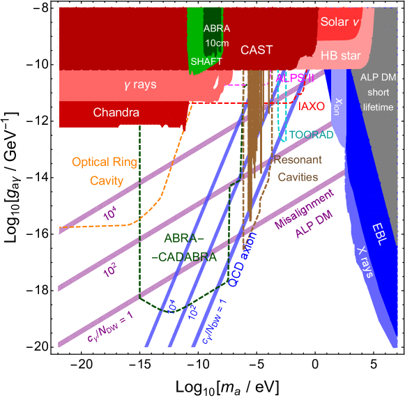
Figure 1: Constraints and future probes on the axion-photon coupling $g_{a\gamma}$. The shaded regions are excluded by the existing laboratory, astrophysics and cosmology bounds, and the dashed lines show the sensitivities of the planned experiments. We also depict $g_{a\gamma}$ of ALP dark matter (pink) and the QCD axion (blue) for three different values of $c_{\gamma}/N_{\rm DW}$, where $N_{\rm DW}=c_{G}$ for the QCD axion.

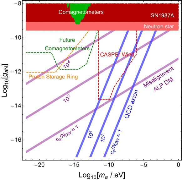
Figure 2: Constraints and future probes on the axion-nucleon coupling $g_{aN}$. The shaded regions are excluded by the existing laboratory and astrophysics bounds, and the dashed lines show the sensitivities of the planned experiments. We also depict $g_{aN}$ of ALP dark matter (pink) and the QCD axion (blue) for three different values of $c_{q}/N_{\rm DW}$, where $N_{\rm DW}=c_{G}$ for the QCD axion.

The CP-conserving axion-photon coupling $g_{a\gamma}$ has been most widely studied for the experimental search for axions. Fig. 1 summarizes the current bounds and future experimental reach for $g_{a\gamma}$ over the vast range of the axion mass $m_{a}$. The axion haloscopes (resonant cavities Sikivie:1983ip ; 2010.00169 ; 1910.11591 ; 2003.10894 , ABRACADABRA 1602.01086 , Optical Ring Cavity 1805.11753 , TOORAD 1807.08810 , see also 2007.15656 for a recent proposal) are based on the hypothesis that axions constitute (certain fraction of) the dark matter (DM) in our Universe. For the axion DM density $\rho_{a}$, their goal is to detect EM waves arising from the axion-induced effective current

$$\begin{split}g_{a\gamma}\partial_{t}a(t)\vec{B}\approx g_{a\gamma}\sqrt{2\rho_{a}}\sin(m_{a}t)\vec{B}.\end{split}$$ (36)

The projected sensitivity limits (dashed lines) in the figure are obtained when $\rho_{a}=\rho_{\rm DM}\simeq 0.4\,\textrm{GeV}/\textrm{cm}^{3}$. Otherwise the limits are to be scaled by the factor $\sqrt{\rho_{a}/\rho_{\rm DM}}$. For comparison, we also display the predicted values of $g_{a\gamma}\sim({\alpha_{\rm em}}/{2\pi})({c_{\gamma}}/{f_{a}})$ for two specific type of axions with $c_{\gamma}/N_{\rm DW}=1,\,10^{2},\,10^{4}$: i) ALP DM with $\rho_{a}=\rho_{\rm DM}$ given by Eq. (12) with $\Theta_{\rm in}=1$, which is produced by the misalignment mechanism (pink lines) and ii) the QCD axion (blue lines). For the QCD axion, we do not specify its cosmological relic abundance since the corresponding blue lines can be determined by Eq. (28) without additional information. Our result shows that for both ALP DM and the QCD axion, the parameter region more easily accessible by the on-going or planned experiments has $c_{\gamma}/N_{\rm DW}\gg 1$, which parametrizes the hierarchy between $g_{a\gamma}\sim({\alpha_{\rm em}}/{2\pi})({c_{\gamma}}/{f_{a}})$ and the coupling $g_{a\Lambda}=N_{\rm DW}/f_{a}$ to generate the leading axion potential ($N_{\rm DW}=c_{G}$ for the QCD axion).

A similar plot for the axion-nucleon coupling $g_{aN}$ is given in Fig. 2 , including experimental sensitivities and the predicted coupling for ALP DM and QCD axion with $c_{q}/N_{\rm DW}=1,\,10^{2},\,10^{4}$. The relevant experiments are CASPEr Wind 1711.08999 , comagnetometers 1709.07852 ; 1907.03767 , and proton storage ring 2005.11867 . They are trying to find the axion DM-induced effective magnetic field interacting with the nucleon spin, whose strength is proportional to

$$\begin{split}g_{aN}\vec{\nabla}a(t,\vec{x})\approx g_{aN}\sqrt{2\rho_{a}}\vec{v}\sin\left(m_{a}t-m_{a}\vec{v}\cdot\vec{x}\right),\end{split}$$ (37)

where $\vec{v}$ ($|\vec{v}|\sim 10^{-3}$) is the axion DM virial velocity with respect to the earth. Again its sensitivity limit in the figure is obtained for $\rho_{a}=\rho_{\rm DM}$, so has to be scaled by the factor $\sqrt{\rho_{a}/\rho_{\rm DM}}$ otherwise. We see that the ALP parameter region more easily probed by those experiments has $c_{q}/N_{\rm DW}\gg 1$, representing the hierarchy between $g_{aN}\sim c_{q}m_{N}/f_{a}$ and $g_{a\Lambda}=N_{\rm DW}/f_{a}$. Although not shown in the figure, recently the QUAX experiment has excluded the axion-electron coupling $g_{ae}\gtrsim 2\times 10^{-11}$ for $m_{a}\simeq 43\,\mu$eV 2001.08940 , which would correspond to $c_{e}/N_{\rm DW}\gtrsim 10^{4}$ for the QCD axion.

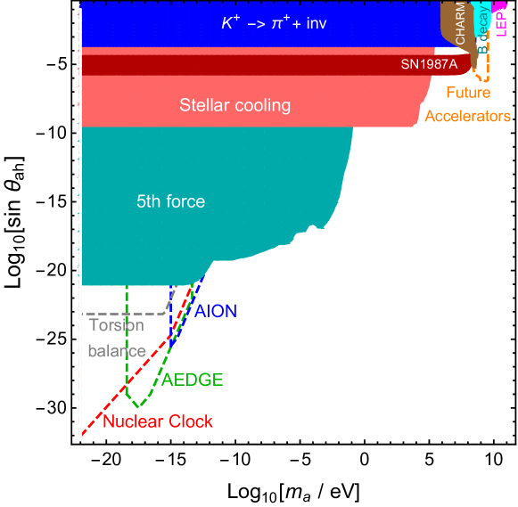
Figure 3: Constraints on the Higgs-axion mixing $\theta_{ah}$ from those on CP-violating axion couplings. The shaded regions are excluded by the existing constraints, while the dashed lines show the sensitivities of future experiments.

There are also a number of bounds and experimental probes on CP-violating axion couplings. As described in Sec. 2.2, such couplings can be induced dominantly by the Higgs-axion mixing Eq. (19), which is indeed the case for the relaxion 1610.00680 ; 1610.02025 ; 2004.02899 . We thus summarize in Fig. 3 the available constraints and future prospect on CP-violating axion couplings in terms of the Higgs-axion mixing angle $\theta_{ah}$. Exhaustive reference lists for them can be found in 2004.02899 ; 1610.00680 ; 1610.02025 ; 2010.03889 . For axions lighter than MeV scale, the constraints are from the axion-mediated 5th force induced by $\bar{g}_{aN}$, stellar cooling by $\bar{g}_{ae}$ 1611.05852 , and supernova (SN1987A) cooling by $\bar{g}_{aN}$. The currently unconstrained supernova trapping window between 100 keV and 30 MeV may be explored by the GANDHI experiment 1810.06467 . Ultralight axion dark matter can be tested by a future nuclear clock experiment 2004.02899 , torsion balances 1512.06165 , and atom interferometers such as AION 1911.11755 and AEDGE 1908.00802 through its CP-violating couplings. These experiments will probe axion DM-induced oscillations of fundamental constants like the electron mass, the nucleon mass, and the fine structure constant via the CP-violating couplings in Eq. (25). So their sensitivities are proportional to the background axion DM field $a(t,x)\approx\sqrt{2\rho_{a}}/m_{a}\cos(m_{a}t)$. The sensitivity lines in the figure are again obtained for $\rho_{a}=\rho_{\rm DM}$. On the other hand, axions heavier than MeV scale are constrained by CHARM beam dump experiment, rare meson decays ($K\rightarrow\pi+a\,[a\rightarrow\textrm{inv}]$, $B\rightarrow K+a\,[a\rightarrow\mu\mu]$), and LEP ($e^{+}e^{-}\rightarrow Z\rightarrow Za$). Heavy axions around GeV scale are to be probed by various future accelerator experiments searching for long-lived particles such as FASER, CODEX-b, SHiP, and MATHUSLA 1710.09387 . For the QCD axion, the dominant source of CP violation is a non-zero $|\theta_{\rm QCD}|<10^{-10}$, which might be too tiny to be probed by the current experiments. Yet ARIADNE experiment 1403.1290 ; 1710.05413 plans to probe $\theta_{\rm QCD}$ several orders of magnitude below $10^{-10}$ by observing the axion-mediated monopole-dipole force $\propto\bar{g}_{aN}g_{aN}$.

2.4.2 Gravitational probes

Gravitational constraints provide a complementary probe of axions. Whereas the non-gravitational probes described in Sec. 2.4.1 constrain axions with relatively heavier masses and stronger couplings, gravitational probes can constrain extremely light axions with large, nearly Planckian, values of $f_{a}/N_{\rm DW}$. Such ultralight axions may constitute a substantial amount of dark energy (DE) or dark matter (DM) as suggested by Eq. (12) while having a large de Broglie wavelength which can have significant cosmological and astrophysical implications. The relevant axion mass range can be classified by three windows: i) DE-like window $m_{a}\lesssim 10^{-27}$ eV, ii) ultralight DM window $10^{-27}\,\textrm{eV}\lesssim m_{a}\lesssim 10^{-19}\,\textrm{eV}$, and iii) black hole (BH) superradiance window $10^{-21}\,\textrm{eV}\lesssim m_{a}\lesssim 10^{-11}\,\textrm{eV}$, which has some overlap with ii). In Fig. 4, we depict the existing constraints and expected future limits from gravitational probes of ultralight DE-like or DM axions produced by the initial misalignment $\Delta a=f_{a}/N_{\rm DW}$, as well as the regions excluded by the black hole (BH) axion superradiance.

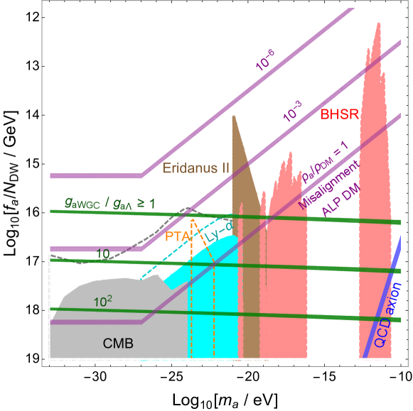
Figure 4: Constraints on the axion scale $f_{a}/N_{\rm DW}$ from gravitational probes. The shaded regions are excluded by the existing constraints, while the dashed lines show the sensitivities of future experiments. Here $f_{a}/N_{\rm DW}$ is identified as the the field excursion $\Delta a$ for ALP DM or DE, and the axion self-interaction scale for BHSR. We also show the axion coupling hierarchy implied by the weak gravity conjecture (green).

For the DE-like window $m_{a}\lesssim 10^{-27}$ eV, the axion field begins to oscillate after the matter-radiation equality and acts as an early DE component. As a result, the locations of the cosmic microwave background (CMB) acoustic peaks shift to larger angular scales (lower $\ell$) and the Universe gets younger. It also increases the largest scale anisotropies through the Integrated Sachs-Wolfe (ISW) effect 1410.2896 . These constrain the amount of axion by the CMB observations as depicted in Fig. 4. For $m_{a}\lesssim 10^{-32}$ eV, the effect of axion on CMB becomes almost indistinguishable from the cosmological constant within the current precision, so the constraint is weakened. If $m_{a}\lesssim 10^{-33}$ eV, the axion field rolls slowly to this day and behaves like the standard DE.

For the ultralight DM window $10^{-27}\,\textrm{eV}\lesssim m_{a}\lesssim 10^{-19}\,\textrm{eV}$, the axion oscillates before the matter-radiation equality, but has a cosmic size of de Broglie wavelength which would affect cosmic structure formation. There are a number of constraints on this mass range from CMB 1708.05681 ; 1806.10608 ; 2003.09655 , pulsar timing array (PTA) 1810.03227 , Lyman-$\alpha$ forest 1708.00015 ; 1611.00036 , and ultra-faint dwarf galaxy (Eridanus II) 1810.08543 , which are depicted in Fig. 4. If $10^{-27}\,\textrm{eV}\lesssim m_{a}\lesssim 10^{-25}\,\textrm{eV}$, the height of the CMB acoustic peaks becomes higher than that of the $\Lambda$CDM because the axion behaves like DE until the time close to the recombination. Moreover, the wave-like property of axion DM suppresses the growth of density perturbation below a certain comoving Jeans scale astro-ph/0003365 ; 1510.07633 , affecting the gravitational lensing of CMB astro-ph/9810092 . Those effects are undiscerned for $m_{a}\gtrsim 10^{-25}$ eV with the current data precision, lifting the CMB constraint. The effects of axion DM on small scales are still significantly constrained by Lyman-$\alpha$ forest data 1708.00015 ; 1611.00036 and by the evolution of dwarf galaxy Eridanus II 1810.08543 , extending the excluded region up to $m_{a}\lesssim 10^{-19}$ eV. While PTA currently puts only a weak constraint on the time-oscillating pressure of axion DM, it may eventually probe the dashed region with a 10 year data set 1810.03227 .

For the BH superradiance window $10^{-21}\,\textrm{eV}\lesssim m_{a}\lesssim 10^{-11}\,\textrm{eV}$, observations of spinning black holes and gravitational waves (GWs) can constrain the existence of axions 0905.4720 ; 1004.3558 . Let us shortly discuss some of the underlying physics for this issue (for the details, see 1501.06570 ). Superradiance is a phenomenon in which incident waves (or bosonic particles) are amplified by extracting energy and angular momentum from a rotating medium. For axion superradiance, a rotating BH provides such a medium. Moreover, because of the gravitational attraction, the emitted axions can form a bound state around the BH, called the axion cloud. This provides a continuous source of incident axions, and can cause an exponential growth of the axion cloud by extracting a substantial fraction of the angular momentum of the BH. In fact, such an amplification of the axion cloud is efficient only when the size of the axion cloud $r_{a}=(\alpha_{g}m_{a})^{-1}$ ($\alpha_{g}\equiv G_{N}M_{\rm BH}m_{a}$) is comparable to the BH size $r_{\rm BH}=G_{N}M_{\rm BH}$, so only for the axion mass window $m_{a}\sim(0.1-1)r_{\rm BH}^{-1}$. Therefore, the observations of highly spinning stellar black holes with $M_{\rm BH}={\cal O}(10M_{\odot})$, the supermassive black holes with $M_{\rm BH}={\cal O}(10^{6}{\rm-}10^{8}M_{\odot})$, and the recently observed spinning M87^∗ with the mass $6.5\times 10^{9}\,M_{\odot}$ provide the strong constraints on the existence of axions in the mass ranges of $10^{-13}{\rm-}10^{-11}\,{\rm eV}$, $10^{-19}{\rm-}10^{-16}\,{\rm eV}$, and $10^{-21}{\rm-}10^{-20}\,{\rm eV}$, respectively. The axion cloud is not absolutely stable. It can emit quasi-monochromatic GWs through axion pair annihilations or level transition. Then the axion mass range $10^{-13}{\rm-}10^{-12}\,{\rm eV}$ is also ruled out by the non-observation of this GW signal in the LIGO/Virgo data.

The above exclusions assume that the superradiant axion modes can grow unhindered to a large enough value. On the other hand, generically axions have a self-interaction provided by the potential, e.g. the quartic coupling $\lambda_{a}\sim-m_{a}^{2}N_{\rm DW}^{2}/f_{a}^{2}$ for Eq. (5), which may interrupt the growth of the axion modes at certain point. If this self-interaction is strong enough, the axion cloud can collapse into the BH before a significant portion of the angular momentum is extracted, creating a GW/axion burst called the bosenova 1004.3558 . Numerical simulations and perturbative estimations indicate that the bosenova occurs for $f_{a}/N_{\rm DW}\lesssim\left({\Delta J}/{G_{N}M_{\rm BH}^{2}}\right)^{1/2}\alpha_{g}^{3/2}M_{P}$, where $\Delta J$ ($\leq G_{N}M_{\rm BH}^{2}$) is the extracted angular momentum of the BH before the collapse. Then, parts of the axion cloud are blown away in the form of GW/axion burst, and the axion cloud will grow again and collapse at some point. If this cycle is repeated many times during the dynamical time scale of the BH, the whole process may take away a large portion of the BH angular momentum. Also, even before the bosenova is triggered, the axion quartic coupling may prevent the exponential growth of the axion cloud and cause early saturation by an efficient energy transfer from the superradiant mode to the damped mode 1604.06422 ; 2011.11646 . Considering those roles of self-interaction, the condition for extracting a sizable amount of the BH angular momentum is approximately given by 1411.2263 ; 2009.07206 ; 2011.11646

$$\begin{split}{\cal O}(10^{15}{\rm-}10^{16}\,{\rm GeV})\min\left[1,\left({10^{-18}\,\textrm{eV}}/{m_{a}}\right)^{1/2}\right]\lesssim f_{a}/N_{\rm DW}.\end{split}$$ (38)

This effect is taken into account in the pink-shaded region in Fig. 4, which is excluded by the BH superradiance. Even when the axion quartic coupling is weak enough to satisfy the above bound, yet the BH superradiance bounds can be avoided if the axion has a hierarchically large coupling to other fields causing an early saturation of the growth of the axion cloud 1910.06308 ; 2004.12326 . This can be due to an axion-dark photon coupling $g_{a\gamma^{\prime}}\gg g_{a\Lambda}=N_{\rm DW}/f_{a}$ which is technically natural and can arise from the clockwork mechanism discussed in Sec. 3.2.

For ultralight DE-like or DM axions, the gravitational probes can reach to a nearly-Planckian value of $f_{a}/N_{\rm DW}$. The corresponding coupling $g_{a\Lambda}=N_{\rm DW}/f_{a}$ might be significantly weaker than the axion-instanton coupling $g_{a{\rm WGC}}$ which is bounded as Eq. (31) by the WGC. To see this, we use Eq. (34) and Eq. (35) with $m_{3/2}\gtrsim 10$ TeV for the bound on $g_{a\rm WGC}$, Eq. (12) with $\Theta_{\rm in}=1$ for the ALP DM density determined by $m_{a}$ and $g_{a\Lambda}=N_{\rm DW}/f_{a}$, and display the resulting $g_{a{\rm WGC}}/g_{a\Lambda}$ in Fig. 4. The observation of a signal below the line of $g_{a{\rm WGC}}/g_{a\Lambda}\geq 1$ would challenge the assumption that the axion potential is dominantly generated by the WGC instanton. However it is yet compatible with the axion WGC which just implies the existence of certain instanton with a coupling $g_{a\rm WGC}\gtrsim S_{I}/M_{P}$ while leaving $g_{a\Lambda}<g_{a\rm WGC}$ as an open possibility. Our result shows that future CMB and PTA observations can probe the region with $g_{a{\rm WGC}}/g_{a\Lambda}\geq 10$.

3 Axions with hierarchical couplings

An interesting feature of axions is that there can be technically natural hierarchies among the couplings of a given axion. Moreover, those hierarchies can have observable consequences. We have seen that, since axions are periodic field, their PQ-breaking couplings are given in terms of integers; for example $g_{a\Lambda}=N_{\rm DW}/f_{a}$. Then the ratios of those quantized couplings do not receive quantum correction. As a consequence, any hierarchy among the PQ-breaking couplings of a given axion can be technically natural, although it may require an explanation for its origin. Also the approximate $U(1)_{\rm PQ}$ symmetry assures that PQ-conserving couplings can be much stronger than PQ-breaking couplings without causing a fine tuning problem. In this section, we present some examples of the well-motivated axion coupling hierarchies and discuss the model building attempts to achieve those hierarchies in low energy effective theory.

3.1 Examples

3.1.1 Coupling hierarchies for the laboratory search for axions

Our first example is the coupling hierarchies relevant for the laboratory search for axions. We already noticed in Sec. 2.4.1 (see Fig. 1 and Fig. 2) that the parameter region of ALP dark matter or the QCD axion which is more easily accessible by the on-going or planned experiments has a bigger hierarchy between $g_{aX}$ ($X=\gamma,N$) and $g_{a\Lambda}$, where $g_{a\Lambda}={N_{\rm DW}}/{f_{a}}$ is the coupling to generate the leading axion potential. To see this, we use Eq. (12), Eq. (2.2) and Eq. (28), and find

$$\begin{split}\hskip-8.5359ptg_{aX}\,\sim\left\{\begin{array}[]{ll}3\times 10^{-12}R_{X}\left(\frac{m_{a}}{\rm eV}\right)^{1/4}\left(\frac{0.1\Theta_{\rm in}^{2}}{\Omega_{a}h^{2}}\right)^{1/2}\,{\rm GeV}^{-1}\quad\mbox{(ALP dark matter)}\\ 10^{-13}R_{X}\left(\frac{m_{a}}{\mu\rm eV}\right)\,{\rm GeV}^{-1}\quad\mbox{(QCD axion)}\end{array},\right.\end{split}$$ (39)

where

$$R_{\gamma}=\frac{\alpha_{\rm em}}{2\pi}\frac{{\rm max}(c_{G},c_{W},c_{B})}{N_{\rm DW}},\quad R_{N}=m_{N}\frac{{\rm max}(c_{G},c_{q})}{N_{\rm DW}}.$$ (40)

The above result shows that for a given axion mass the corresponding $g_{aX}$ has a bigger value for bigger $R_{X}$, so is easier to be detected. These correlations between $g_{aX}$ and $m_{a}$ are displayed by the pink (ALP dark matter) and blue (QCD axion) lines in Fig. 1 and Fig. 2 for three different values of the hierarchy factor $R_{X}$ determined by $c_{\gamma}/N_{\rm DW}=(c_{W}+c_{B})/N_{\rm DW}=1,10^{2},10^{4}$ and $c_{q}/N_{\rm DW}=1,10^{2},10^{4}$. For ALP dark matter, $\rho_{a}=\rho_{\rm DM}$ and $\Theta_{\rm in}=1$ are also assumed.

Another interesting possibility is that one of $g_{aX}$ ($X=\gamma,N,e$) is much stronger than the others, e.g. i) the photophilic limit with $c_{B,W}\gg c_{G,q}$ 1512.05295 ; 1611.09855 ; 1709.06085 ; 2008.02279 ; 2010.15846 , ii) the nucleophilic limit with $c_{q}\gg c_{G,W,B}$ 1803.07575 ; 2008.02279 ; 2010.15846 , and iii) the leptophilic limit with $c_{e}\gg c_{G,q}$ 2007.08834 ; 2010.15846 . Since most of the axion search experiments are designed to be sensitive to one specific coupling, these limits also might be more easily probed by the on-going or planned experiments. Yet, the natural range of these parameter hierarchies are limited by the renormalization group mixings between $c_{X}$ ($X=G,W,B$) and $c_{\Psi}$ ($\Psi=q,e$) induced by the SM interactions, for instance Eq. (18). Also, at scales around the nucleon or electron mass, the 1PI axion-photon coupling $g_{a\gamma}$ receives a threshold correction $\delta g_{a\gamma}={\cal O}\Big{(}\frac{\alpha_{\rm em}}{2\pi}\frac{p_{a}^{2}}{m_{\Psi}^{2}}\frac{g_{a\Psi}}{m_{\Psi}}\Big{)}$ from the axion-fermion coupling $g_{a\Psi}$ ($\Psi=e,N$), where $p_{a}$ denotes the axion 4-momentum. Taking those quantum corrections into account, we find the following naturalness bounds on the possible hierarchies among $g_{aX}$ ($X=\gamma,N,e$):

$$\hskip-17.07182pt\mbox{Photophilic limit:}\quad 1\,\ll\,\frac{c_{W,B}}{c_{q,G}}\,\sim\,\frac{2\pi m_{N}}{\alpha_{\rm em}}\frac{g_{a\gamma}}{g_{aN}}\,\lesssim\,{\cal O}\left(\frac{4\pi^{2}}{\alpha_{\rm em}^{2}}\frac{1}{\ln(f_{a}/m_{N})}\right),$$

$$\hskip-17.07182pt\mbox{Nucleophilic limit:}\quad 1\,\ll\,\frac{c_{q}}{c_{B,W,G}+{\cal O}(p_{a}^{2}c_{q}/m_{N}^{2})}\,\sim\,\frac{\alpha_{\rm em}}{2\pi m_{N}}\frac{g_{aN}}{g_{a\gamma}}\,\lesssim\,{\cal O}\left(\frac{m_{N}^{2}}{p_{a}^{2}}\right),$$

$$\hskip-17.07182pt\mbox{Leptophilic limit:}\quad 1\,\ll\,\frac{c_{e}}{c_{G,q}}\,\sim\,\frac{m_{N}}{m_{e}}\frac{g_{ae}}{g_{aN}}\,\lesssim\,{\cal O}\left(\frac{4\pi^{2}}{\alpha_{\rm em}^{2}}\frac{1}{\ln(f_{a}/m_{N})}\right).$$ (41)

3.1.2 Coupling hierarchy for the relaxion

In the relaxion solution to the weak scale hierarchy problem, which was briefly described in Sec. 2.1.3, the technically unnatural hierarchy between $v=246$ GeV and the Higgs mass cutoff scale $\Lambda_{H}$ is traded for a technically natural but much bigger hierarchy between the relaxion couplings. For instance, for the original model with $\Lambda_{\rm br}\lesssim v$ 1504.07551 , the relaxion stabilization condition Eq. (14) leads to

$$\begin{split}\frac{g_{a{\rm br}}}{g_{a\Lambda}}=\frac{N_{\rm br}}{N_{\rm DW}}\sim\frac{\Lambda^{4}}{\Lambda_{\rm br}^{4}}\gtrsim\frac{\Lambda_{H}^{4}}{v^{4}}\end{split}$$ (42)

where $g_{a\Lambda}=N_{\rm DW}/f_{a}$ and $g_{a{\rm br}}=N_{\rm br}/f_{a}$ are the relaxion couplings to generate $V_{0}$ and $V_{\rm br}$ in the relaxion potential Eq. (13).

Similar hierarchy is required for different models which exploit different mechanisms to dissipate away the relaxion kinetic energy 1507.07525 ; 1607.01786 ; 1805.04543 ; 1811.06520 ; 1904.02545 ; 1909.07706 ; 1911.08473 . Here we consider two examples in which the dissipation is dominated by bosonic particle production 1607.01786 ; 1911.08473 . As the Hubble friction is negligible in these examples, the relaxion initial velocity can be greater than the barrier height as $\dot{a}_{0}>\Lambda_{\rm br}^{2}$. Yet the relaxion can efficiently lose its kinetic energy by developing non-homogeneous modes (i.e. producing relaxion quanta), which is dubbed “relaxion fragmentation” 1911.08473 . The relaxion will eventually be trapped at a local potential minimum when its velocity drops below the barrier height. Successful implementation of the relaxion fragmentation requires

$$\begin{split}\frac{g_{a{\rm br}}}{g_{a\Lambda}}=\frac{N_{\rm br}}{N_{\rm DW}}\sim\max\left[\frac{\Lambda^{4}}{\Lambda_{\rm br}^{4}}\times\frac{\dot{a}_{0}^{2}}{\Lambda_{\rm br}^{4}},\,\frac{\Lambda_{1}^{2}}{v^{2}}\times\frac{\dot{a}_{0}^{4}}{\Lambda_{\rm br}^{8}}\right]\gtrsim\frac{\Lambda_{H}^{4}}{v^{4}}\end{split}$$ (43)

with $\dot{a}_{0}\gtrsim\Lambda_{\rm br}^{2}$ and $\Lambda_{\rm br}\lesssim v$, which is comparable or stronger than the hierarchy Eq. (42).

Tachyonic production of light gauge bosons can also serve as a friction for the relaxion 1607.01786 ; 1911.08473 . Contrary to the above scenarios, here the Higgs vacuum value is initially of ${\cal O}(\Lambda_{H})$ and later relaxed to the observed weak scale. The relaxion is coupled to the electroweak gauge bosons as Eq. (17), but with $c_{W}=-c_{B}$ to avoid the coupling to the photon. Initially the $W/Z$ bosons are heavy and their production is negligible. As the Higgs vacuum value is relaxed to the observed one, these bosons become light enough to be produced by the rolling relaxion, causing the relaxion to lose its kinetic energy and eventually stop the excursion. Regarding the axion coupling hierarchy, this model requires

$$\begin{split}\frac{g_{a{\rm br}}}{g_{a\Lambda}}=\frac{N_{\rm br}}{N_{\rm DW}}>\max\left[\frac{\Lambda_{H}^{4}}{\Lambda_{\rm br}^{4}},\,\frac{\Lambda_{H}^{2}}{v^{2}}\right]\end{split}$$ (44)

in order for the relaxion to scan the Higgs mass with enough precision. The key difference from other scenarios is that in this case $\Lambda_{\rm br}$ is independent of the Higgs field, so can be bigger than $v$. Then the above coupling hierarchy can be significantly weaker than those in other scenarios. On the other hand, there can be additional coupling hierarchy in this scenario due to the coupling to the electroweak gauge bosons: $c_{W}/8\pi^{2}f_{a}=-c_{B}/8\pi^{2}f_{a}\sim{v}/{\dot{a}_{0}}$.

3.1.3 Coupling hierarchies for large field excursion

Our next example is the coupling hierarchy associated with the axion WGC hep-th/0601001 ; 1412.3457 ; 1503.00795 ; 1503.03886 ; 1503.04783 . As discussed in Sec. 2.1, some well-motivated axions can have a large cosmological field excursion $\sim 1/g_{a\Lambda}=f_{a}/N_{\rm DW}$ comparable to $M_{P}$ or even bigger. Since the axion-instanton coupling $g_{a{\rm WGC}}$ suggested by the WGC is bounded as Eq. (31), for such axions there can be a coupling hierarchy with

$$g_{a{\rm WGC}}\gg g_{a\Lambda}.$$ (45)

As concrete examples, one may consider i) axion inflation with $f_{a}/N_{\rm DW}\sim\sqrt{N_{e}}M_{P}$ and $m_{a}\sim{\cal H}_{\rm inf}/\sqrt{N_{e}}$, which is presented in Sec. 2.1.1, ii) axion-like dark energy (quintesence) with $f_{a}/N_{\rm DW}\sim M_{P}$ and $m_{a}\sim 10^{-33}$ eV, and iii) ultralight ALP dark matter produced by the initial misalignment $\sim\Theta_{\rm in}f_{a}/N_{\rm DW}$, whose relic energy density is given by Eq. (12). Applying the WGC bound Eq. (31) to these cases, we find

$$\begin{split}\hskip-8.5359pt\frac{g_{a{\rm WGC}}}{g_{a\Lambda}}\,\gtrsim\,S_{I}\frac{f_{a}/N_{\rm DW}}{M_{P}}\sim\left\{\begin{array}[]{ll}\sqrt{N_{e}}S_{I}\quad\mbox{(axion inflation)}\\ \quad S_{I}\quad\quad\mbox{(quintessence axion)}\\ \Big{(}\frac{S_{I}}{20}\Big{)}\Big{(}\frac{10^{-22}{\rm eV}}{m_{a}}\Big{)}^{1/4}\Big{(}\frac{\Omega_{a}h^{2}}{0.1\Theta_{\rm in}^{2}}\Big{)}^{1/2}\,\,\,\mbox{(ALP dark matter)}\end{array}.\right.\end{split}$$

For numerical estimate of the above coupling hierarchy, one may use Eq. (34) and Eq. (35) together with $m_{3/2}\sim{\cal H}_{\rm inf}\sim 10^{13}$ GeV during the early Universe inflation and $m_{3/2}\gtrsim 10$ TeV in the present universe. One then find that roughly $g_{a{\rm WGC}}/g_{a\Lambda}\gtrsim 10^{2}$ for axion inflation and quintessence axion, and $g_{a{\rm WGC}}/g_{a\Lambda}\gtrsim 10$ for ALP dark matter with $m_{a}\sim 10^{-22}$ and $\Omega_{a}h^{2}\sim 0.1$ 1807.00824 that may explain the small scale problems of the cold dark matter scenario astro-ph/0003365 ; 1610.08297 . It is also an interesting possibility that ultralight axions with $m_{a}\ll 10^{-22}$ constitute a small but non-negligible fraction of dark matter, e.g. $\Omega_{a}h^{2}\sim 10^{-2}$, which would leave an observable imprint in future cosmological data. Such a case also results in $g_{a{\rm WGC}}/g_{a\Lambda}\gg 1$. In Fig. 4, the value of $g_{a{\rm WGC}}/g_{a\Lambda}$ is shown over the parameter region where the gravitational effects of ultralight ALP dark matter can be probed by astrophysical or cosmological observations in near future.

3.1.4 Coupling hierarchies with other cosmological or astrophysical motivations

In addition to the examples presented above, the coupling hierarchy $g_{a\gamma}\gg\frac{\alpha_{\rm em}}{2\pi}g_{a\Lambda}$ or a similar hierarchy between $g_{a\Lambda}$ and the axion coupling to dark gauge bosons has been exploited with a variety of different cosmological or astrophysical motivations. Because of the space limitation, here we simply list those works without any further discussion. They include the coupling hierarchy for the magnetogenesis Turner:1987bw ; hep-ph/9209238 ; 1802.07269 , dissipative inflation 0908.4089 ; 1608.06223 , chromonatural inflation 1202.2366 ; 1806.09621 , reducing the abundance of the QCD axion dark matter 1708.05008 ; 1711.06590 , production of dark photon dark matter 1810.07188 ; 1810.07196 , ALP-photon-dark photon oscillations to explain the tentative EDGES signal of 21-cm photons 1911.00532 , avoiding the BH superradiance bounds on axion masses 2004.12326 , and resonant photon emission from the mergers of axion stars/oscillons 2009.11337 .

3.2 Hierarchies from axion landscape

In this subsection, we discuss the model building attempts to generate hierarchical axion couplings in low energy effective theory without having hierarchical parameters in the underlying UV theory. Most of the coupling hierarchies discussed in the previous subsection are those among the quantized PQ-breaking couplings, therefore involve a large integer-valued parameter, e.g. $c_{B,W}\gg 1$ for a photophilic axion and $N_{\rm br}\gg 1$ for the relaxion. Even when all UV parameters have the values of order unity, such a large integer may appear in low energy effective theory as a consequence of introducing a large number of fields in the UV theory hep-th/0507205 ; 1511.00132 ; 1511.01827 ; 1512.05295 ; 1610.07962 ; 1611.09855 ; 1404.6209 ; 1404.6923 ; 1404.7496 ; 1504.03566 ; 1704.07831 ; 1709.01080 ; 1709.06085 ; 1711.06228 ; 1806.09621 . Yet, different models can have different efficiencies, i.e. the resulting hierarchy grows differently w.r.t. the number of introduced fields. Here we focus on the scheme based on the axion landscape provided by the potential of many $(N_{H}\gg 1)$ massive axions. We will explain that this scheme can generate an exponential hierarchy of ${\cal O}(e^{N_{H}})$ among the effective couplings of light axions after the massive axions are integrated out.

Let us start with a generic effective lagrangian of multiple axions:

$$\hskip-14.22636pt{\cal L}=\frac{1}{2}f^{2}_{ij}\partial_{\mu}\theta^{i}\partial^{\mu}\theta^{j}-V(\theta^{i})+\frac{k_{Xi}\theta^{i}}{32\pi^{2}}F^{X\mu\nu}{\tilde{F}}^{X}_{\mu\nu}+c_{\psi i}\partial_{\mu}\theta^{i}\bar{\psi}\bar{\sigma}^{\mu}\psi+\cdots,$$ (46)

where $\theta^{i}\cong\theta^{i}+2\pi$ ($i=1,2,\cdots,N$), $k_{Xi}$ are integer-valued coefficients, and the summation over the repeated indices $i,X,\psi$ are understood. The axion potential $V$ arises as a consequence of the breakdown of the PQ symmetries $[U(1)_{\rm PQ}]^{N}:\theta^{i}\rightarrow\theta^{i}+c^{i}$ $\left(c^{i}={\rm constants}\right)$. For $p$-form zero mode axions such as Eq. (3), often the corresponding PQ symmetries are broken only by non-perturbative effects Dine:1986zy ; hep-ph/9902292 ; hep-th/0605206 ; 1610.08297 , yielding $V\propto e^{-b/g_{*}^{2}}$ for some coupling $g_{*}$. For accidental PQ symmetries, their violations are suppressed by certain powers of $1/M_{P}$ Barr:1992qq ; hep-th/9202003 ; hep-ph/9203206 , which would result in $V\propto(f/M_{P})^{n}$ for $f\ll M_{P}$. These suggest that generically axion potentials with different origin have hierarchically different size, giving hierarchical axion masses. Then, at a given energy scale, some axions can be heavy enough to be frozen at their vacuum values, while the other light axions are allowed to have a dynamical evolution over their entire field range. To describe such a situation, we will analyze here a simplified model in which the axion potential has two distinct scales, $\Lambda_{A}$ and $\Lambda_{a}$, with $\Lambda_{A}\gg\Lambda_{a}$. The physics we describe will be the same for models with a range of large and small energy scales, as long as these are well separated. We write the axion potential, then, as

$$V\,=\,V_{H}+V_{L}\,=\,-\sum_{A=1}^{N_{H}}\Lambda_{A}^{4}\cos(q^{A}_{i}\theta^{i})-\sum_{a=1}^{N_{L}}\Lambda_{a}^{4}\cos(p^{a}_{i}\theta^{i})\quad(\Lambda_{A}\gg\Lambda_{a}),$$ (47)

where $\vec{q}^{\,A}=(q^{A}_{1},\cdots,q^{A}_{N})$ ($A=1,\cdots,N_{H}$) and $\vec{p}^{\,a}=(p^{a}_{1},\cdots,p^{a}_{N})$ ($a=1,\cdots,N_{L}$) with $N_{L}=N-N_{H}$ are linearly independent integer-valued vectors. For simplicity, here we consider the simple cosine potentials including only the dominant term for each linearly independent axion combination. However our discussion does not rely on this specific potential and applies for generic periodic axion potentials. In this system, considered in the low energy limit, the heavy axion combinations $q^{A}_{i}\theta^{i}$ are frozen at the vacuum state of $V_{H}$. The light degrees of freedom are given by the $N_{L}$ axions parametrizing the directions that are not constrained by $V_{H}$. As we will see, the resulting effective theory of those light axions can have rich structures including various coupling hierarchies and enlarged field ranges.

The effective lagrangian Eq. (46) is defined in the field basis for which the discrete symmetry to ensure the periodic nature of axions is given by

$$\mathbb{Z}^{N}:\,\,\,\theta^{i}\,\rightarrow\,\theta^{i}+2\pi\ell^{i}\quad(\ell^{i}\in\mathbb{Z}).$$ (48)

However, in the regime where the axion mass hierarchies become important, it is more convenient to use a different field basis minimizing the mixing between the axions with hierarchically different masses. To find such a field basis, we first decompose $q^{A}_{i}$ into the Smith normal form smith1861 :

$$q^{A}_{i}=\sum_{B}\hat{U}^{A}_{\,\,B}\lambda_{B}\hat{q}^{B}_{i},$$ (49)

where $\lambda_{A}\in\mathbb{Z}$, $\hat{U}=[\hat{U}^{A}_{\,\,B}]\in GL(N_{H},\mathbb{Z})$, $\hat{q}=[\hat{q}^{A}_{i},\hat{q}^{a}_{i}]\in GL(N,\mathbb{Z})$. Here $\hat{U}$ and $\hat{q}$ are integer-valued and invertible matrices whose inverses are also integer-valued, and therefore $|\det\hat{U}|=|\det\hat{q}|=1$. Then the desired field basis is obtained by the $GL(N,\mathbb{Z})$ rotation:

$$\theta_{H}^{A}=\hat{q}^{A}_{i}\theta^{i},\quad\theta_{L}^{a}=\hat{q}^{a}_{i}\theta^{i},$$ (50)

followed by the field redefinition:

$$\theta_{H}^{A}\,\,\rightarrow\,\,\theta_{H}^{A},\quad\theta^{a}_{L}\,\,\rightarrow\,\,\theta^{a}_{L}+\hat{q}^{a}_{i}(f^{-2})^{ij}\hat{q}^{A}_{j}(f^{2}_{H})_{AB}\theta_{H}^{B},$$ (51)

where $f^{2}_{ij}(f^{-2})^{jk}=\delta^{k}_{i}$ and $(f^{2}_{H})_{AB}$ is defined in Eq. (55). With this, $\theta^{i}$ are parameterized as

$$\theta^{i} = \hat{n}_{a}^{i}\Big{(}\theta_{L}^{a}+\hat{q}^{a}_{j}(f^{-2})^{jk}\hat{q}_{k}^{A}(f_{H}^{2})_{AB}\theta_{H}^{B}\Big{)}+\hat{n}^{i}_{B}\theta_{H}^{B}$$ (52)

$$= \hat{n}^{i}_{a}\theta^{a}_{L}+(f^{-2})^{ij}\hat{q}^{A}_{j}(f_{H}^{2})_{AB}\theta_{H}^{B},$$

where the integers $\hat{n}^{i}_{a}$ are given by the $N_{L}\times N$ submatrix of the inverse of $\hat{q}$:

$$\hat{q}^{-1}=\left[\hat{n}^{i}_{A},~{}\hat{n}^{i}_{a}\right]^{T}.$$ (53)

Note that, since an inverse is involved here, the integers $\hat{n}^{i}_{a}$ can be large even when all of $q^{A}_{i}$ are of order unity. This will play an important role below.

Applying the above parameterization to the lagrangian Eq. (46), we obtain

$$\hskip-8.5359pt{\cal L} = \frac{1}{2}(f^{2}_{L})_{ab}\partial_{\mu}\theta_{L}^{a}\partial^{\mu}\theta_{L}^{b}+\frac{1}{2}(f^{2}_{H})_{AB}\partial_{\mu}\theta_{H}^{A}\partial^{\mu}\theta_{H}^{B}$$ (54)

$$+ \Lambda_{A}^{4}\cos(\hat{U}^{A}_{B}\lambda_{B}\theta_{H}^{B})+\Lambda_{a}^{4}\cos\Big{(}p^{a}_{i}\hat{n}^{i}_{b}\theta_{L}^{b}+p^{a}_{i}(f^{-2})^{ij}\hat{q}^{A}_{j}(f^{2}_{H})_{AB}\theta_{H}^{B}\Big{)}$$

$$+ \frac{1}{32\pi^{2}}\Big{(}k_{Xi}\hat{n}^{i}_{a}\theta_{L}^{a}+k_{Xi}(f^{-2})^{ij}\hat{q}^{A}_{j}(f^{2}_{H})_{AB}\theta_{H}^{B}\Big{)}F^{X}_{\mu\nu}\tilde{F}^{X\mu\nu}$$

$$+ \Big{(}c_{\psi i}\hat{n}^{i}_{a}\partial_{\mu}\theta^{a}_{L}+c_{\psi i}(f^{-2})^{ij}\hat{q}^{A}_{j}(f^{2}_{H})_{AB}\partial_{\mu}\theta_{H}^{B}\Big{)}\bar{\psi}\bar{\sigma}^{\mu}\psi+\cdots$$

with the block-diagonalized kinetic metric given by

$$(f_{L}^{2})_{ab}=\hat{n}_{a}^{i}f^{2}_{ij}\hat{n}_{b}^{j},\quad(f^{2}_{H})_{AB}(f_{H}^{-2})^{BC}=\delta^{A}_{C}\ \ {\rm for}\ \ (f^{-2}_{H})^{AB}=\hat{q}^{A}_{i}(f^{-2})^{ij}\hat{q}^{B}_{j}.$$ (55)

It shows that in the new field basis the mixings between the heavy axions $\theta_{H}^{A}$ and the light axions $\theta_{L}^{a}$ are suppressed by $\Lambda_{a}^{4}/\Lambda_{A}^{4}\ll 1$, so can be ignored. On the other hand, the discrete symmetry Eq. (48) takes a more complicate form as $\mathbb{Z}^{N}=\mathbb{Z}^{N_{L}}\times\mathbb{Z}^{N_{H}}$ with

$$\hskip-28.45274pt\mathbb{Z}^{N_{L}}:\,\,\,\theta_{L}^{a}\rightarrow\theta_{L}^{a}+2\pi\ell^{a},$$

$$\hskip-28.45274pt\mathbb{Z}^{N_{H}}:\,\,\,\theta_{H}^{A}\rightarrow\theta_{H}^{A}+2\pi\ell^{A},\,\,\,\theta_{L}^{a}\rightarrow\theta_{L}^{a}-2\pi\ell^{A}\hat{q}^{a}_{i}(f^{-2})^{ij}\hat{q}^{B}_{j}(f_{H}^{2})_{BA},$$ (56)

for $\ell^{a},\ell^{A}\in\mathbb{Z}$. This implies that while $\theta_{L}^{a}$ are $2\pi$-periodic by themselves, $\theta_{H}^{A}$ are $2\pi$-periodic modulo the shifts of light axions $\Delta\theta_{L}^{a}=2\pi\hat{q}^{a}_{i}(f^{-2})^{ij}\hat{q}^{B}_{j}(f_{H}^{2})_{BA}$. As a result, for a gauge field strength $F^{X}_{\mu\nu}$ which couples to the light axions $\theta_{L}^{a}$, the couplings of $\theta_{H}^{A}$ to $F^{X}_{\mu\nu}\tilde{F}^{X\mu\nu}$ are generically non-quantized, while the couplings of $\theta_{L}^{a}$ remain to be quantized.

Our major concern is the possibility to generate a hierarchy among the low energy couplings of the light axions $\theta_{L}^{a}$ without introducing hierarchical parameters in the underlying UV model. Prior to the discussion of this issue, we make a small digression to mention the coupling hierarchy of $\theta_{H}^{A}$ noticed in 1709.06085 , which relies on the hierarchical structure of the original axion scales $f^{2}_{ij}$, so has different characteristics than the coupling hierarchies of $\theta_{L}^{a}$ that will be discussed later. If $f^{2}_{ij}$ have hierarchical eigenvalues and $\hat{q}^{A}_{i}$ is well aligned with the large eigenvalue direction while having a sizable mixing with the small eigenvalue direction, there exists a parameter region with $\langle\theta_{H}^{A}|\theta^{i}\rangle=(f^{-2})^{ij}\hat{q}^{B}_{j}(f_{H}^{2})_{BA}\gg 1$ for some $i,A$. It can enhance the coupling of $\theta_{H}^{A}$ to gauge fields relative to the coupling to generate the leading potential. A simple example is the photophilic QCD axion model discussed in 1709.06085 , involving two axions with

$$f^{2}_{ij}=\left(\begin{array}[]{cc}f_{1}^{2}&\epsilon f_{1}f_{2}\\ \epsilon f_{1}f_{2}&f_{2}^{2}\end{array}\right),\quad\vec{q}^{\,A}=(0,1),\quad\vec{k}_{\gamma}=(k_{1},k_{2}),$$ (59)

where $f_{2}>\epsilon f_{2}\gg f_{1}$, $q^{A}_{i}=\hat{q}^{A}_{i}$ is the coupling of $\theta^{i}$ to the gluon anomaly generating the QCD axion potential as the last term in Eq. (27), and $k_{\gamma i}$ is the coupling to the photon. Then $a(x)=f_{H}\theta_{H}^{A}(x)$ ($\theta_{H}^{A}=\theta_{2}$, $f_{H}\simeq f_{2}$) can be identified as the QCD axion with a decay constant $f_{H}$, whose coupling to the photon is enhanced as

$$g_{a\gamma}\simeq\frac{\epsilon f_{2}}{f_{1}}\frac{\alpha_{\rm em}}{2\pi}\frac{k_{1}}{f_{H}}\gg\frac{\alpha_{\rm em}}{2\pi}g_{a\Lambda}=\frac{\alpha_{\rm em}}{2\pi}\frac{1}{f_{H}}.$$ (60)

Let us now come back to the main issue. To examine the low energy couplings of $\theta_{L}^{a}$, we integrate out the heavy axions $\theta_{H}^{A}$. Ignoring the small corrections of ${\cal O}(\Lambda_{a}^{4}/\Lambda_{A}^{4})$, the vacuum solution of heavy axions is given by $\theta_{H}^{A}=0$ for arbitrary background of $\theta_{L}^{a}$. Applying it to Eq. (52), the vacuum manifiold of $V_{H}$ is parameterized as

$$\theta^{i}=\hat{n}_{a}^{i}\theta_{L}^{a},$$ (61)

and the effective lagrangian of the corresponding light axions is given by

$${\cal L}_{\rm eff} = \frac{1}{2}(f^{2}_{L})_{ab}\partial_{\mu}\theta_{L}^{a}\partial^{\mu}\theta_{L}^{b}+\Lambda_{a}^{4}\cos(p^{a}_{i}\hat{n}^{i}_{b}\theta_{L}^{b})$$ (62)

$$+ \frac{k_{Xi}\hat{n}^{i}_{a}\theta_{L}^{a}}{32\pi^{2}}F^{X}\tilde{F}^{X}+c_{\psi i}\hat{n}^{i}_{a}\partial_{\mu}\theta^{a}_{L}\bar{\psi}\bar{\sigma}^{\mu}\psi+\cdots.$$

This effective lagrangian suggests that even when the UV lagrangian Eq. (46) does not involve any hierarchical parameter, e.g. all dimensionless parameters in Eq. (46) are of order unity and also all eigenvalues of $f^{2}_{ij}$ have a similar size, if $|\hat{n}_{a}|\gg 1$ could be obtained from $\vec{q}^{\,A}$ with $|\vec{q}^{\,A}|={\cal O}(1)$, the light axion couplings can have a hierarchical pattern determined by the relative angles between $\hat{n}_{a}$ and $\{\vec{p}^{\,a},\vec{k}_{X},\vec{c}_{\psi}\}$. Another consequence of $|\hat{n}_{a}|\gg 1$ is that the light axion decay constants are enlarged as $(f_{L})^{2}_{ab}=\hat{n}^{i}_{a}f^{2}_{ij}\hat{n}^{j}_{b}\gg f^{2}_{ij}$.

In fact, $|\hat{n}_{a}|\gg 1$ is a generic feature of the axion landscape scenario with $N_{H}\gg N_{L}$ 1404.6209 ; 1404.6923 . To see this, we first note that block diagonalization of the axion kinetic terms by Eq. (52) leads to the following identity for the field space volume of the canonically normalized axions:

$$\det(f_{L}^{2})\det(f_{H}^{2})=\det(f^{2}).$$ (63)

We also find

$$\det(\hat{n}_{a}\cdot\hat{n}_{b})=\det(\hat{q}^{A}\cdot\hat{q}^{B}),$$ (64)

where $\hat{n}_{a}=(\hat{n}_{a}^{1},\cdots,\hat{n}_{a}^{N})$ and $\hat{q}^{A}=(\hat{q}^{A}_{1},\cdots,\hat{q}^{A}_{N})$. This relation can be obtained from Eq. (63) by taking $f^{2}_{ij}=f_{0}^{2}\delta_{ij}$, but is valid independently of $f^{2}_{ij}$. We can further take an average of this relation over the Gaussian distribution of $\hat{q}^{A}_{i}$, and find goodman1963

$$\Big{\langle}\det(\hat{n}_{a}\cdot\hat{n}_{b})\Big{\rangle}=\left\langle\det(\hat{q}^{A}\cdot\hat{q}^{B})\right\rangle\sim\left\langle|\hat{q}|^{2}\right\rangle^{N_{H}}\quad(N_{H}\gg 1),$$ (65)

where $|\hat{q}|^{2}=\sum_{A,i}(\hat{q}^{A}_{i})^{2}/N_{H}$. Unless $\hat{q}^{A}_{i}$ have a highly specific form like $\hat{q}^{A}_{i}=\delta^{A}_{i}$, we have $|\hat{q}|^{2}>1$. Then, Eq. (65) implies that in the limit $N_{H}\gg N_{L}$ the generic value of $|\hat{n}_{a}|$ is exponentially large as

$$|\hat{n}_{a}|\sim|\hat{q}|^{N_{H}/N_{L}}$$ (66)

where $|\hat{q}|$ ($>1$) is comparable to the typical value of $|\vec{q}^{\,A}|/{\rm gcd}(\vec{q}^{\,A})$. With this, the light axion decay constants are exponentially enlarged as $f_{L}\sim|\hat{q}|^{N_{H}/N_{L}}f$, and also the effective couplings of $\theta_{L}^{a}$ can have an exponential hierarchy determined by the relative angles between $\hat{n}_{a}$ and $\{\vec{p}^{\,a},\vec{k}_{X},\vec{c}_{\psi}\}$. We stress that this is the consequence of the periodic nature of axions which requires that all components of $\hat{n}_{a}$ are integer-valued. As they represent the degenerate vacuum solution of $V_{H}=-\Lambda_{A}^{4}\cos(q^{A}_{i}\theta^{i})$, $\hat{n}_{a}$ should be orthogonal to $N_{H}$ linearly-independent $\vec{q}^{\,A}$s. However, when $N_{H}\gg N_{L}$, it is exponentially difficult for $\hat{n}_{a}$ to point in the right direction with only ${\cal O}(1)$ integer-valued components, so typically $|\hat{n}_{a}|$ are forced to have exponentially large values.

So far, we have discussed the generic feature of the axion landscape scenario which can be relevant for axion coupling hierarchies. Let us now proceed with explicit examples. For simplicity, we consider the case of single light axion ($N_{L}=1$), for which 1404.6209

$$\hat{n}^{i}\equiv\hat{n}_{a}^{i}=\frac{1}{{\rm gcd}(\vec{\cal N})}{\cal N}^{i}\quad{\rm with}\quad{\cal N}^{i}=\det\left(\begin{array}[]{ccc}\delta^{i}_{\,1}&\cdots&\delta^{i}_{\,N}\\ q^{1}_{1}&\cdots&q^{1}_{N}\\ \vdots&\ddots&\vdots\\ \,q^{N_{H}}_{1}&\cdots&\,\,q^{N_{H}}_{N}\end{array}\right).$$ (71)

Our first example is a two axion model ($N_{H}=N_{L}=1$) realizing the mechanism for enlarging the monotonic field range of the light axion described in hep-ph/0409138 ; 1404.7127 , called the KNP alignment. The relevant model parameters of our example are given by

$$f^{2}_{ij}=f_{0}^{2}\delta_{ij},\quad\vec{q}^{\,A}=\vec{q}=(q_{1},q_{2}),\quad\vec{p}^{\,a}=\vec{p}=(p_{1},p_{2}),$$ (72)

where $\vec{q}^{\,A}$ and $\vec{p}^{\,a}$ determine $V_{H}$ and $V_{L}$ as Eq. (47). Then the canonically normalized light axion component and its potential are determined as

$$a_{L}=f_{0}\frac{{\hat{n}\cdot\vec{\theta}}}{|\hat{n}|},\quad V_{L}=-\Lambda_{a}^{4}\cos\left(g_{a\Lambda}a_{L}\right)=-\Lambda_{a}^{4}\cos\Big{(}\frac{\hat{n}\cdot\vec{p}}{|\hat{n}|f_{0}}a_{L}\Big{)}$$ (73)

with

$$\hat{n}=\frac{1}{{\rm gcd}(q_{1},q_{2})}(q_{2},-q_{1}).$$ (74)

The monotonic field range of the light axion potential, i.e. $\Delta a_{L}=1/g_{a\Lambda}=f_{0}|\hat{n}|/|\hat{n}\cdot\vec{p}|$, becomes much bigger than the original scale $f_{0}$ in the KNP alignment limit where $\vec{q}$ and $\vec{p}$ are aligned to be nearly parallel, giving $0<|\hat{n}\cdot\vec{p}|\ll|\hat{n}|$. If any of $\vec{q}$ and $\vec{p}$ were a real-valued vector, such an alignment could be made with $|\vec{q}|={\cal O}(1)$. However for periodic axions, both $\vec{q}$ and $\vec{p}$ are integer-valued, so $|\hat{n}\cdot\vec{p}|=0$ or $\geq 1$. Accordingly, the KNP alignment requires $|\vec{q}|\geq|\hat{n}|\gg 1$. This implies that the KNP mechanism can yield $\Delta a_{L}\gg f_{0}$ and also the coupling hierarchies, but at the expense of introducing a large integer-valued input parameter.

The original motivation of the KNP mechanism is to get $\Delta a_{L}>M_{P}$ starting from a UV model with $f_{0}\ll M_{P}$ hep-ph/0409138 . It has been widely discussed that such a trans-Planckian field range obtained by the KNP mechanism may have a conflict with the axion WGC. In those discussions applied to the model of Eq. (72), one often identifies $\vec{g}_{aH}=\vec{q}/f_{0}$ and $\vec{g}_{aL}=\vec{p}/f_{0}$ as the axion-instanton couplings spanning the convex hull constrained by the WGC, and find that the corresponding convex hull cannot satisfy Eq. (31) while giving $\Delta a_{L}=f_{0}|\hat{n}|/|\hat{n}\cdot\vec{p}|>M_{P}$ 1503.00795 ; 1503.03886 ; 1503.04783 ; 1504.00659 ; 1506.03447 ; 1607.06814 . However, as noticed in Sec. 2.3, in our viewpoint the axion WGC just implies the existence of certain instanton couplings whose convex hull satisfies Eq. (31), but it does not require that the axion potential is determined dominantly by those instanton couplings 1412.3457 ; 1503.04783 ; 1504.00659 ; 1608.06951 . This allows that the model Eq. (72) gives rise to $\Delta a_{L}>M_{P}$ without any conflict with the axion WGC. Yet, the axion WGC indicates that there exists an instanton with the coupling $\vec{g}_{\cal I}=\vec{p}_{\cal I}/f_{0}$ not aligned with $\vec{g}_{aH}=\vec{q}/f_{0}$, which makes a negligible contribution to the axion potential. Then, $\Delta a_{L}>M_{P}$ can be obtained through the KNP alignment of $\vec{g}_{aH}=\vec{q}/f_{a}$ and $\vec{g}_{aL}=\vec{p}/f_{a}$, while the WGC condition Eq. (31) is fulfilled by the convex hull spanned by $\vec{g}_{aH}=\vec{q}/f_{0}$ and $\vec{g}_{a\cal I}=\vec{p}_{\cal I}/f_{0}$. In such case, the two effective couplings of the light axion $a_{L}$, i.e. $g_{a\Lambda}=|\hat{n}\cdot\vec{p}|/|\hat{n}|f_{0}<1/M_{P}$ and $g_{a{\rm WGC}}=|\hat{n}\cdot\vec{p}_{\cal I}|/|\hat{n}|f_{0}>S_{I}/M_{P}$ have hierarchically different size 1511.05560 ; 1511.07201 .

A potential drawback of the KNP model is that it requires a large integer-valued input parameter to have $|\vec{q}^{\,A}|\gg 1$. Our discussion leading to Eq. (65) implies that this drawback disappears in models with many axions. Statistical analysis also suggests that the scheme becomes more efficient with a larger number of axions 1404.6209 ; 1404.6923 . In the case with $N$ ($\gg 1$) axions, the model can be defined on the linear quiver hep-th/0104005 with $N$ sites for the angular axions $\theta^{i}\cong\theta^{i}+2\pi$. One may then assume that axion couplings in the quiver involve only the nearest two sites. Taking this assumption, the $N_{H}=N-1$ linearly independent couplings to generate the heavy axion potential are given by

$$q^{A}_{i}=q_{A}\delta^{A}_{i}-q^{\prime}_{A}\delta^{A}_{i-1}\quad(q_{A},q^{\prime}_{A}\in\mathbb{Z}).$$ (75)

Among such models, a particularly interesting example is the clockwork axion model 1404.6209 ; 1511.00132 ; 1511.01827 with

$$f^{2}_{ij}=f_{0}^{2}\delta_{ij},\quad q_{A}=q,\quad q^{\prime}_{A}=1\quad\forall\,\,\,A.$$ (76)

The clockwork mechanism naturally arranges that

$$\hat{n}=(1,q,q^{2},\cdots,q^{N-1}).$$ (77)

Note that in the quiver description, $\hat{n}_{a}^{i}$ can be interpreted as the wavefuntion profile of the light axion along the linear quiver, with which many of the low energy properties of the light axion can be understood 1704.07831 .

To examine the effective couplings of the light axion $a_{L}=f_{0}\hat{n}\cdot\vec{\theta}/|\hat{n}|$ in the clockwork axion model, let us introduce the following additional couplings:

$$\vec{g}_{a\Lambda}=\frac{\vec{p}}{f_{0}},\quad\vec{g}_{a{\cal I}}=\frac{\vec{p}_{\cal I}}{f_{0}},\quad\vec{g}_{aX}=\frac{g_{X}^{2}}{8\pi^{2}}\frac{\vec{k}_{X}}{f_{0}},$$ (78)

where $\vec{g}_{a\Lambda}$ is the coupling to generate the leading potential of the light axion, $\vec{g}_{a{\cal I}}$ is a coupling to generate additional but subleading potential, e.g. the coupling to the WGC instanton satisfying the bound Eq. (31) or the coupling for the barrier potential $V_{\rm br}$ of the relaxion, and $\vec{g}_{aX}$ is the coupling to $F^{X}_{\mu\nu}\tilde{F}^{X\mu\nu}$. For the integer-valued $\vec{p},\vec{p}_{\cal I}$ and $\vec{k}_{X}$, one can again assume that they involve at most the nearest two sites in the quiver. Here we choose the simplest option involving a specific single site as it gives essentially the same result:

$$p_{i}=\delta^{N_{1}}_{i},\quad p_{{\cal I}i}=\delta^{N_{2}}_{i},\quad k_{Xi}=\delta^{N_{3}}_{i},$$ (79)

where $1\leq N_{\ell}\leq N$ ($\ell=1,2,3$). Then the low energy effective couplings of the light axion are given by

$${g_{a\Lambda}}=\frac{\hat{n}\cdot\vec{g}_{a\Lambda}}{|\hat{n}|}\,=\,\frac{q^{N_{1}-1}}{f_{L}},\quad g_{aX}=\frac{g^{2}_{X}}{8\pi^{2}}\frac{\hat{n}\cdot\vec{g}_{aX}}{|\hat{n}|}\,=\,\frac{g^{2}_{X}}{8\pi^{2}}\frac{q^{N_{3}-1}}{f_{L}},$$

$$g_{a{\cal I}}=\frac{\hat{n}\cdot\vec{g}_{a{\cal I}}}{|\hat{n}|}\,=\,\frac{q^{N_{2}-1}}{f_{L}},\quad({\cal I}=\mbox{WGC or br})$$ (80)

with an exponentially enlarged decay constant

$$f_{L}=|\hat{n}|f_{0}=\sqrt{\frac{q^{2N}-1}{q^{2}-1}}f_{0}\sim q^{N-1}f_{0}.$$ (81)

The above results show that with appropriately chosen $1\leq N_{\ell}\leq N$, the model can have an exponentially enlarged monotonic field range $\Delta a_{L}=1/g_{a\Lambda}\sim q^{N-N_{1}}f_{0}$ of the light axion, which can be trans-Planckian while satisfying the WGC bound Eq. (31) with $g_{a{\rm WGC}}={\cal O}(1/f_{0})\gg g_{a\Lambda}$. The model also exhibits a variety of exponential hierarchies among the low energy axion couplings. We also note that the exponentially enlarged $\Delta a_{L}\propto q^{N-N_{1}}$ can easily overcome the possible suppression of $f_{0}\propto 1/N^{p}$ ($p=3-4$) which was observed for some string theory axions in 1808.01282 . It turns out that the above clockwork mechanism can be generalized to the fields with nonzero spin to generate various parameter hierarchies in particle physics 1610.07962 . It also has the continuum limit $N\rightarrow\infty$ leading to an extra-dimensional realization of the clockwork mechanism 1610.07962 ; 1704.07831 ; 1711.06228 . Although interesting, these generalizations are beyond the scope of this review.

4 Summary and conclusion

Axions have rich physical consequences described by a variety of coupling or scale parameters. Those parameters include for instance i) the coupling $g_{a\Lambda}$ that generates the leading term in the axion potential, which defines the monotonic field range of the potential and also the possible cosmological excursion of the axion field, ii) the couplings to the SM particles, particularly those to the photon, nucleon and electron, and iii) the axion-instanton couplings suggested by the weak gravity conjecture. An interesting feature of the axion parameter space is that there can be hierarchies among the different couplings of a given axion, which have good physics motivations and at the same time are technically natural. For instance, the parameter regions that are most accessible by the on-going or planned axion search experiments, including the astrophysical and cosmological observations, often correspond to regions where the axion couplings have large hierarchies. The hierarchy between $g_{a\Lambda}$ and the axion couplings to the gauge fields in the SM or hidden sector has been exploited with a variety of different cosmological or astrophysical motivations. The relaxion idea to solve the weak scale hierarchy problem essentially trades the technically unnatural hiearchy between the weak scale and the cutoff scale for a technically natural but typically bigger hierarchy between $g_{a\Lambda}$ and other relaxion couplings. Taking the WGC bound on certain axion-instanton couplings, a tran-Planckian (or nearly Planckian) axion field excursion may imply a hierarchy between $g_{a\Lambda}$ and the couplings to the WGC instantons.

In this paper, we have reviewed the recent developments in axion physics while giving particular attention to the subjects of hierarchies between axion couplings. We first summarized the existing observational constraints on axion couplings, as well as the projected sensitivity limits of the planned experiments, which are displayed in Figs. 1 - 4. For comparison, we also show in the figures the parameter ratios which exhibit certain axion coupling hierarchies. It is apparent that the parameter regions of greatest experimental interest require large hierarchies between the axion couplings. In the theory of axions, such hierarchies are always technically natural. But it is important to show also that these hierarchies can follow from simple model-building mechanisms. Therefore, after presenting the examples of well-motivated axion coupling hierarchies, we discussed the model building attempts to generate hierarchical axion couplings in low energy effective theory. We have focused on a specific scheme that is based on a landscape of many axions, and we have shown that the required coupling hierarchies appear naturally in this setting. The presence of many axions with very different scales of their potentials is common in string theory, so this scheme might be realized in certain corner in the string landscape. The scheme is quite efficient. It can generate an exponential hierarchy among the low energy axion couplings with appropriately chosen ${\cal O}(1)$ integer-valued parameters in the UV theory. The ideas connected with axion coupling hierarchies mesh in a very attractive way with the regions of the axion parameter space that will be probed in the near future by on-going and planned experiments.

References

- (1) J. E. Kim and G. Carosi, “Axions and the Strong CP Problem,” Rev. Mod. Phys. 82 (2010) 557–602, arXiv:0807.3125 [hep-ph]. [Erratum: Rev.Mod.Phys. 91, 049902 (2019)].
- (2) D. J. E. Marsh, “Axion Cosmology,” Phys. Rept. 643 (2016) 1–79, arXiv:1510.07633 [astro-ph.CO].
- (3) L. Di Luzio, M. Giannotti, E. Nardi, and L. Visinelli, “The landscape of QCD axion models,” Phys. Rept. 870 (2020) 1–117, arXiv:2003.01100 [hep-ph].
- (4) P. Svrcek and E. Witten, “Axions In String Theory,” JHEP 06 (2006) 051, arXiv:hep-th/0605206.
- (5) A. Arvanitaki, S. Dimopoulos, S. Dubovsky, N. Kaloper, and J. March-Russell, “String Axiverse,” Phys. Rev. D 81 (2010) 123530, arXiv:0905.4720 [hep-th].
- (6) R. D. Peccei and H. R. Quinn, “CP Conservation in the Presence of Instantons,” Phys. Rev. Lett. 38 (1977) 1440–1443.
- (7) S. Weinberg, “A New Light Boson?,” Phys. Rev. Lett. 40 (1978) 223–226.
- (8) F. Wilczek, “Problem of Strong and Invariance in the Presence of Instantons,” Phys. Rev. Lett. 40 (1978) 279–282.
- (9) K. Freese, J. A. Frieman, and A. V. Olinto, “Natural inflation with pseudo - Nambu-Goldstone bosons,” Phys. Rev. Lett. 65 (1990) 3233–3236.
- (10) P. W. Graham, D. E. Kaplan, and S. Rajendran, “Cosmological Relaxation of the Electroweak Scale,” Phys. Rev. Lett. 115 no. 22, (2015) 221801, arXiv:1504.07551 [hep-ph].
- (11) J. Preskill, M. B. Wise, and F. Wilczek, “Cosmology of the Invisible Axion,” Phys. Lett. B 120 (1983) 127–132.
- (12) L. F. Abbott and P. Sikivie, “A Cosmological Bound on the Invisible Axion,” Phys. Lett. B 120 (1983) 133–136.
- (13) M. Dine and W. Fischler, “The Not So Harmless Axion,” Phys. Lett. B 120 (1983) 137–141.
- (14) P. Arias, D. Cadamuro, M. Goodsell, J. Jaeckel, J. Redondo, and A. Ringwald, “WISPy Cold Dark Matter,” JCAP 06 (2012) 013, arXiv:1201.5902 [hep-ph].
- (15) M. Meyer, D. Horns, and M. Raue, “First lower limits on the photon-axion-like particle coupling from very high energy gamma-ray observations,” Phys. Rev. D 87 no. 3, (2013) 035027, arXiv:1302.1208 [astro-ph.HE].
- (16) A. H. Córsico, A. D. Romero, L. G. Althaus, E. García-Berro, J. Isern, S. O. Kepler, M. M. Miller Bertolami, D. J. Sullivan, and P. Chote, “An asteroseismic constraint on the mass of the axion from the period drift of the pulsating DA white dwarf star L19-2,” JCAP 07 (2016) 036, arXiv:1605.06458 [astro-ph.SR].
- (17) K. Kohri and H. Kodama, “Axion-Like Particles and Recent Observations of the Cosmic Infrared Background Radiation,” Phys. Rev. D 96 no. 5, (2017) 051701, arXiv:1704.05189 [hep-ph].
- (18) K. Choi and S. H. Im, “Constraints on Relaxion Windows,” JHEP 12 (2016) 093, arXiv:1610.00680 [hep-ph].
- (19) T. Flacke, C. Frugiuele, E. Fuchs, R. S. Gupta, and G. Perez, “Phenomenology of relaxion-Higgs mixing,” JHEP 06 (2017) 050, arXiv:1610.02025 [hep-ph].
- (20) A. Banerjee, H. Kim, O. Matsedonskyi, G. Perez, and M. S. Safronova, “Probing the Relaxed Relaxion at the Luminosity and Precision Frontiers,” JHEP 07 (2020) 153, arXiv:2004.02899 [hep-ph].
- (21) P. W. Graham, I. G. Irastorza, S. K. Lamoreaux, A. Lindner, and K. A. van Bibber, “Experimental Searches for the Axion and Axion-Like Particles,” Ann. Rev. Nucl. Part. Sci. 65 (2015) 485–514, arXiv:1602.00039 [hep-ex].
- (22) I. G. Irastorza and J. Redondo, “New experimental approaches in the search for axion-like particles,” Prog. Part. Nucl. Phys. 102 (2018) 89–159, arXiv:1801.08127 [hep-ph].
- (23) P. Sikivie, “Invisible Axion Search Methods,” Rev. Mod. Phys. 93 no. 1, (2021) 015004, arXiv:2003.02206 [hep-ph].
- (24) D. Grin, M. A. Amin, V. Gluscevic, R. Hlǒzek, D. J. E. Marsh, V. Poulin, C. Prescod-Weinstein, and T. L. Smith, “Gravitational probes of ultra-light axions,” arXiv:1904.09003 [astro-ph.CO].
- (25) N. Arkani-Hamed, L. Motl, A. Nicolis, and C. Vafa, “The String landscape, black holes and gravity as the weakest force,” JHEP 06 (2007) 060, arXiv:hep-th/0601001.
- (26) A. de la Fuente, P. Saraswat, and R. Sundrum, “Natural Inflation and Quantum Gravity,” Phys. Rev. Lett. 114 no. 15, (2015) 151303, arXiv:1412.3457 [hep-th].
- (27) T. Rudelius, “Constraints on Axion Inflation from the Weak Gravity Conjecture,” JCAP 09 (2015) 020, arXiv:1503.00795 [hep-th].
- (28) M. Montero, A. M. Uranga, and I. Valenzuela, “Transplanckian axions!?,” JHEP 08 (2015) 032, arXiv:1503.03886 [hep-th].
- (29) J. Brown, W. Cottrell, G. Shiu, and P. Soler, “Fencing in the Swampland: Quantum Gravity Constraints on Large Field Inflation,” JHEP 10 (2015) 023, arXiv:1503.04783 [hep-th].
- (30) P. Saraswat, “Weak gravity conjecture and effective field theory,” Phys. Rev. D 95 no. 2, (2017) 025013, arXiv:1608.06951 [hep-th].
- (31) J. E. Kim, H. P. Nilles, and M. Peloso, “Completing natural inflation,” JCAP 01 (2005) 005, arXiv:hep-ph/0409138.
- (32) S. Dimopoulos, S. Kachru, J. McGreevy, and J. G. Wacker, “N-flation,” JCAP 08 (2008) 003, arXiv:hep-th/0507205.
- (33) K. Choi, H. Kim, and S. Yun, “Natural inflation with multiple sub-Planckian axions,” Phys. Rev. D 90 (2014) 023545, arXiv:1404.6209 [hep-th].
- (34) K. Choi and S. H. Im, “Realizing the relaxion from multiple axions and its UV completion with high scale supersymmetry,” JHEP 01 (2016) 149, arXiv:1511.00132 [hep-ph].
- (35) D. E. Kaplan and R. Rattazzi, “Large field excursions and approximate discrete symmetries from a clockwork axion,” Phys. Rev. D 93 no. 8, (2016) 085007, arXiv:1511.01827 [hep-ph].
- (36) G. F. Giudice and M. McCullough, “A Clockwork Theory,” JHEP 02 (2017) 036, arXiv:1610.07962 [hep-ph].
- (37) M. Farina, D. Pappadopulo, F. Rompineve, and A. Tesi, “The photo-philic QCD axion,” JHEP 01 (2017) 095, arXiv:1611.09855 [hep-ph].
- (38) P. Agrawal, J. Fan, M. Reece, and L.-T. Wang, “Experimental Targets for Photon Couplings of the QCD Axion,” JHEP 02 (2018) 006, arXiv:1709.06085 [hep-ph].
- (39) J. E. Kim, “Weak Interaction Singlet and Strong CP Invariance,” Phys. Rev. Lett. 43 (1979) 103.
- (40) M. A. Shifman, A. I. Vainshtein, and V. I. Zakharov, “Can Confinement Ensure Natural CP Invariance of Strong Interactions?,” Nucl. Phys. B 166 (1980) 493–506.
- (41) M. Dine, W. Fischler, and M. Srednicki, “A Simple Solution to the Strong CP Problem with a Harmless Axion,” Phys. Lett. B 104 (1981) 199–202.
- (42) A. R. Zhitnitsky, “On Possible Suppression of the Axion Hadron Interactions. (In Russian),” Sov. J. Nucl. Phys. 31 (1980) 260.
- (43) E. Witten, “Some Properties of O(32) Superstrings,” Phys. Lett. B 149 (1984) 351–356.
- (44) K. Choi, “String or M theory axion as a quintessence,” Phys. Rev. D 62 (2000) 043509, arXiv:hep-ph/9902292.
- (45) T. Banks, M. Dine, P. J. Fox, and E. Gorbatov, “On the possibility of large axion decay constants,” JCAP 06 (2003) 001, arXiv:hep-th/0303252.
- (46) K. Choi and J. E. Kim, “Harmful Axions in Superstring Models,” Phys. Lett. B 154 (1985) 393. [Erratum: Phys.Lett.B 156, 452 (1985)].
- (47) Planck Collaboration, Y. Akrami et al., “Planck 2018 results. X. Constraints on inflation,” Astron. Astrophys. 641 (2020) A10, arXiv:1807.06211 [astro-ph.CO].
- (48) S. Borsanyi et al., “Calculation of the axion mass based on high-temperature lattice quantum chromodynamics,” Nature 539 no. 7627, (2016) 69–71, arXiv:1606.07494 [hep-lat].
- (49) L. Hui, J. P. Ostriker, S. Tremaine, and E. Witten, “Ultralight scalars as cosmological dark matter,” Phys. Rev. D 95 no. 4, (2017) 043541, arXiv:1610.08297 [astro-ph.CO].
- (50) H. Georgi, D. B. Kaplan, and L. Randall, “Manifesting the Invisible Axion at Low-energies,” Phys. Lett. B 169 (1986) 73–78.
- (51) E. Silverstein and A. Westphal, “Monodromy in the CMB: Gravity Waves and String Inflation,” Phys. Rev. D 78 (2008) 106003, arXiv:0803.3085 [hep-th].
- (52) M. Srednicki, “Axion Couplings to Matter. 1. CP Conserving Parts,” Nucl. Phys. B 260 (1985) 689–700.
- (53) S. Chang and K. Choi, “Hadronic axion window and the big bang nucleosynthesis,” Phys. Lett. B 316 (1993) 51–56, arXiv:hep-ph/9306216.
- (54) D. B. Kaplan, “Opening the Axion Window,” Nucl. Phys. B 260 (1985) 215–226.
- (55) H. Leutwyler and M. A. Shifman, “GOLDSTONE BOSONS GENERATE PECULIAR CONFORMAL ANOMALIES,” Phys. Lett. B 221 (1989) 384–388.
- (56) R. S. Chivukula, A. G. Cohen, H. Georgi, and A. V. Manohar, “Couplings of a Light Higgs Boson,” Phys. Lett. B 222 (1989) 258–262.
- (57) G. Grilli di Cortona, E. Hardy, J. Pardo Vega, and G. Villadoro, “The QCD axion, precisely,” JHEP 01 (2016) 034, arXiv:1511.02867 [hep-ph].
- (58) S. Borsanyi, Z. Fodor, C. Hoelbling, L. Lellouch, K. K. Szabo, C. Torrero, and L. Varnhorst, “Ab-initio calculation of the proton and the neutron’s scalar couplings for new physics searches,” arXiv:2007.03319 [hep-lat].
- (59) J. E. Moody and F. Wilczek, “NEW MACROSCOPIC FORCES?,” Phys. Rev. D 30 (1984) 130.
- (60) S. Bertolini, L. Di Luzio, and F. Nesti, “Axion-mediated forces, CP violation and left-right interactions,” Phys. Rev. Lett. 126 no. 8, (2021) 081801, arXiv:2006.12508 [hep-ph].
- (61) J. F. Gunion, G. Gamberini, and S. F. Novaes, “Can the Higgs Bosons of the Minimal Supersymmetric Model Be Detected at a Hadron Collider via Two Photon Decays?,” Phys. Rev. D 38 (1988) 3481.
- (62) E. Palti, “The Swampland: Introduction and Review,” Fortsch. Phys. 67 no. 6, (2019) 1900037, arXiv:1903.06239 [hep-th].
- (63) C. Cheung and G. N. Remmen, “Naturalness and the Weak Gravity Conjecture,” Phys. Rev. Lett. 113 (2014) 051601, arXiv:1402.2287 [hep-ph].
- (64) M. Dine, N. Seiberg, X. G. Wen, and E. Witten, “Nonperturbative Effects on the String World Sheet,” Nucl. Phys. B 278 (1986) 769–789.
- (65) J. Brown, W. Cottrell, G. Shiu, and P. Soler, “On Axionic Field Ranges, Loopholes and the Weak Gravity Conjecture,” JHEP 04 (2016) 017, arXiv:1504.00659 [hep-th].
- (66) B. Heidenreich, M. Reece, and T. Rudelius, “Weak Gravity Strongly Constrains Large-Field Axion Inflation,” JHEP 12 (2015) 108, arXiv:1506.03447 [hep-th].
- (67) A. Hebecker, P. Mangat, S. Theisen, and L. T. Witkowski, “Can Gravitational Instantons Really Constrain Axion Inflation?,” JHEP 02 (2017) 097, arXiv:1607.06814 [hep-th].
- (68) R. Blumenhagen, M. Cvetic, S. Kachru, and T. Weigand, “D-Brane Instantons in Type II Orientifolds,” Ann. Rev. Nucl. Part. Sci. 59 (2009) 269–296, arXiv:0902.3251 [hep-th].
- (69) P. Sikivie, “Experimental Tests of the Invisible Axion,” Phys. Rev. Lett. 51 (1983) 1415–1417. [Erratum: Phys.Rev.Lett. 52, 695 (1984)].
- (70) ADMX Collaboration, R. Khatiwada et al., “Axion Dark Matter eXperiment: Detailed Design and Operations,” arXiv:2010.00169 [astro-ph.IM].
- (71) Y. K. Semertzidis et al., “Axion Dark Matter Research with IBS/CAPP,” arXiv:1910.11591 [physics.ins-det].
- (72) S. Beurthey et al., “MADMAX Status Report,” arXiv:2003.10894 [physics.ins-det].
- (73) Y. Kahn, B. R. Safdi, and J. Thaler, “Broadband and Resonant Approaches to Axion Dark Matter Detection,” Phys. Rev. Lett. 117 no. 14, (2016) 141801, arXiv:1602.01086 [hep-ph].
- (74) I. Obata, T. Fujita, and Y. Michimura, “Optical Ring Cavity Search for Axion Dark Matter,” Phys. Rev. Lett. 121 no. 16, (2018) 161301, arXiv:1805.11753 [astro-ph.CO].
- (75) D. J. E. Marsh, K.-C. Fong, E. W. Lentz, L. Smejkal, and M. N. Ali, “Proposal to Detect Dark Matter using Axionic Topological Antiferromagnets,” Phys. Rev. Lett. 123 no. 12, (2019) 121601, arXiv:1807.08810 [hep-ph].
- (76) A. Berlin, R. T. D’Agnolo, S. A. R. Ellis, and K. Zhou, “Heterodyne Broadband Detection of Axion Dark Matter,” arXiv:2007.15656 [hep-ph].
- (77) D. F. Jackson Kimball et al., “Overview of the Cosmic Axion Spin Precession Experiment (CASPEr),” Springer Proc. Phys. 245 (2020) 105–121, arXiv:1711.08999 [physics.ins-det].
- (78) P. W. Graham, D. E. Kaplan, J. Mardon, S. Rajendran, W. A. Terrano, L. Trahms, and T. Wilkason, “Spin Precession Experiments for Light Axionic Dark Matter,” Phys. Rev. D 97 no. 5, (2018) 055006, arXiv:1709.07852 [hep-ph].
- (79) I. M. Bloch, Y. Hochberg, E. Kuflik, and T. Volansky, “Axion-like Relics: New Constraints from Old Comagnetometer Data,” JHEP 01 (2020) 167, arXiv:1907.03767 [hep-ph].
- (80) P. W. Graham, S. Hacıömeroğlu, D. E. Kaplan, Z. Omarov, S. Rajendran, and Y. K. Semertzidis, “Storage ring probes of dark matter and dark energy,” Phys. Rev. D 103 no. 5, (2021) 055010, arXiv:2005.11867 [hep-ph].
- (81) QUAX Collaboration, N. Crescini et al., “Axion search with a quantum-limited ferromagnetic haloscope,” Phys. Rev. Lett. 124 no. 17, (2020) 171801, arXiv:2001.08940 [hep-ex].
- (82) C. A. J. O’Hare and E. Vitagliano, “Cornering the axion with CP-violating interactions,” Phys. Rev. D 102 (2020) 115026, arXiv:2010.03889 [hep-ph].
- (83) E. Hardy and R. Lasenby, “Stellar cooling bounds on new light particles: plasma mixing effects,” JHEP 02 (2017) 033, arXiv:1611.05852 [hep-ph].
- (84) G. Benato, A. Drobizhev, S. Rajendran, and H. Ramani, “Invisible decay modes in nuclear gamma cascades,” Phys. Rev. D 99 no. 3, (2019) 035025, arXiv:1810.06467 [hep-ph].
- (85) P. W. Graham, D. E. Kaplan, J. Mardon, S. Rajendran, and W. A. Terrano, “Dark Matter Direct Detection with Accelerometers,” Phys. Rev. D 93 no. 7, (2016) 075029, arXiv:1512.06165 [hep-ph].
- (86) L. Badurina et al., “AION: An Atom Interferometer Observatory and Network,” JCAP 05 (2020) 011, arXiv:1911.11755 [astro-ph.CO].
- (87) AEDGE Collaboration, Y. A. El-Neaj et al., “AEDGE: Atomic Experiment for Dark Matter and Gravity Exploration in Space,” EPJ Quant. Technol. 7 (2020) 6, arXiv:1908.00802 [gr-qc].
- (88) J. L. Feng, I. Galon, F. Kling, and S. Trojanowski, “Dark Higgs bosons at the ForwArd Search ExpeRiment,” Phys. Rev. D 97 no. 5, (2018) 055034, arXiv:1710.09387 [hep-ph].
- (89) A. Arvanitaki and A. A. Geraci, “Resonantly Detecting Axion-Mediated Forces with Nuclear Magnetic Resonance,” Phys. Rev. Lett. 113 no. 16, (2014) 161801, arXiv:1403.1290 [hep-ph].
- (90) ARIADNE Collaboration, A. A. Geraci et al., “Progress on the ARIADNE axion experiment,” Springer Proc. Phys. 211 (2018) 151–161, arXiv:1710.05413 [astro-ph.IM].
- (91) R. Hlozek, D. Grin, D. J. E. Marsh, and P. G. Ferreira, “A search for ultralight axions using precision cosmological data,” Phys. Rev. D 91 no. 10, (2015) 103512, arXiv:1410.2896 [astro-ph.CO].
- (92) R. Hlozek, D. J. E. Marsh, and D. Grin, “Using the Full Power of the Cosmic Microwave Background to Probe Axion Dark Matter,” Mon. Not. Roy. Astron. Soc. 476 no. 3, (2018) 3063–3085, arXiv:1708.05681 [astro-ph.CO].
- (93) V. Poulin, T. L. Smith, D. Grin, T. Karwal, and M. Kamionkowski, “Cosmological implications of ultralight axionlike fields,” Phys. Rev. D 98 no. 8, (2018) 083525, arXiv:1806.10608 [astro-ph.CO].
- (94) J. B. Bauer, D. J. E. Marsh, R. Hložek, H. Padmanabhan, and A. Laguë, “Intensity Mapping as a Probe of Axion Dark Matter,” Mon. Not. Roy. Astron. Soc. 500 no. 3, (2020) 3162–3177, arXiv:2003.09655 [astro-ph.CO].
- (95) N. K. Porayko et al., “Parkes Pulsar Timing Array constraints on ultralight scalar-field dark matter,” Phys. Rev. D 98 no. 10, (2018) 102002, arXiv:1810.03227 [astro-ph.CO].
- (96) T. Kobayashi, R. Murgia, A. De Simone, V. Iršič, and M. Viel, “Lyman- constraints on ultralight scalar dark matter: Implications for the early and late universe,” Phys. Rev. D 96 no. 12, (2017) 123514, arXiv:1708.00015 [astro-ph.CO].
- (97) DESI Collaboration, A. Aghamousa et al., “The DESI Experiment Part I: Science,Targeting, and Survey Design,” arXiv:1611.00036 [astro-ph.IM].
- (98) D. J. E. Marsh and J. C. Niemeyer, “Strong Constraints on Fuzzy Dark Matter from Ultrafaint Dwarf Galaxy Eridanus II,” Phys. Rev. Lett. 123 no. 5, (2019) 051103, arXiv:1810.08543 [astro-ph.CO].
- (99) W. Hu, R. Barkana, and A. Gruzinov, “Cold and fuzzy dark matter,” Phys. Rev. Lett. 85 (2000) 1158–1161, arXiv:astro-ph/0003365.
- (100) U. Seljak and M. Zaldarriaga, “Measuring dark matter power spectrum from cosmic microwave background,” Phys. Rev. Lett. 82 (1999) 2636–2639, arXiv:astro-ph/9810092.
- (101) A. Arvanitaki and S. Dubovsky, “Exploring the String Axiverse with Precision Black Hole Physics,” Phys. Rev. D 83 (2011) 044026, arXiv:1004.3558 [hep-th].
- (102) R. Brito, V. Cardoso, and P. Pani, “Superradiance: New Frontiers in Black Hole Physics,” Lect. Notes Phys. 906 (2015) pp.1–237, arXiv:1501.06570 [gr-qc].
- (103) A. Gruzinov, “Black Hole Spindown by Light Bosons,” arXiv:1604.06422 [astro-ph.HE].
- (104) M. Baryakhtar, M. Galanis, R. Lasenby, and O. Simon, “Black hole superradiance of self-interacting scalar fields,” arXiv:2011.11646 [hep-ph].
- (105) A. Arvanitaki, M. Baryakhtar, and X. Huang, “Discovering the QCD Axion with Black Holes and Gravitational Waves,” Phys. Rev. D 91 no. 8, (2015) 084011, arXiv:1411.2263 [hep-ph].
- (106) M. J. Stott, “Ultralight Bosonic Field Mass Bounds from Astrophysical Black Hole Spin,” arXiv:2009.07206 [hep-ph].
- (107) H. Fukuda and K. Nakayama, “Aspects of Nonlinear Effect on Black Hole Superradiance,” JHEP 01 (2020) 128, arXiv:1910.06308 [hep-ph].
- (108) A. Mathur, S. Rajendran, and E. H. Tanin, “Clockwork mechanism to remove superradiance limits,” Phys. Rev. D 102 no. 5, (2020) 055015, arXiv:2004.12326 [hep-ph].
- (109) T. Higaki, K. S. Jeong, N. Kitajima, and F. Takahashi, “The QCD Axion from Aligned Axions and Diphoton Excess,” Phys. Lett. B 755 (2016) 13–16, arXiv:1512.05295 [hep-ph].
- (110) J. A. Dror and J. M. Leedom, “Cosmological Tension of Ultralight Axion Dark Matter and its Solutions,” Phys. Rev. D 102 no. 11, (2020) 115030, arXiv:2008.02279 [hep-ph].
- (111) L. Darmé, L. Di Luzio, M. Giannotti, and E. Nardi, “Selective enhancement of the QCD axion couplings,” Phys. Rev. D 103 no. 1, (2021) 015034, arXiv:2010.15846 [hep-ph].
- (112) G. Marques-Tavares and M. Teo, “Light axions with large hadronic couplings,” JHEP 05 (2018) 180, arXiv:1803.07575 [hep-ph].
- (113) C. Han, M. L. López-Ibáñez, A. Melis, O. Vives, and J. M. Yang, “Anomaly-free leptophilic axionlike particle and its flavor violating tests,” Phys. Rev. D 103 no. 3, (2021) 035028, arXiv:2007.08834 [hep-ph].
- (114) E. Hardy, “Electroweak relaxation from finite temperature,” JHEP 11 (2015) 077, arXiv:1507.07525 [hep-ph].
- (115) A. Hook and G. Marques-Tavares, “Relaxation from particle production,” JHEP 12 (2016) 101, arXiv:1607.01786 [hep-ph].
- (116) N. Fonseca, E. Morgante, and G. Servant, “Higgs relaxation after inflation,” JHEP 10 (2018) 020, arXiv:1805.04543 [hep-ph].
- (117) S.-J. Wang, “Paper-boat relaxion,” Phys. Rev. D 99 no. 9, (2019) 095026, arXiv:1811.06520 [hep-ph].
- (118) M. Ibe, Y. Shoji, and M. Suzuki, “Fast-Rolling Relaxion,” JHEP 11 (2019) 140, arXiv:1904.02545 [hep-ph].
- (119) K. Kadota, U. Min, M. Son, and F. Ye, “Cosmological Relaxation from Dark Fermion Production,” JHEP 02 (2020) 135, arXiv:1909.07706 [hep-ph].
- (120) N. Fonseca, E. Morgante, R. Sato, and G. Servant, “Relaxion Fluctuations (Self-stopping Relaxion) and Overview of Relaxion Stopping Mechanisms,” JHEP 05 (2020) 080, arXiv:1911.08473 [hep-ph]. [Erratum: JHEP 01, 012 (2021)].
- (121) A. Hebecker, T. Mikhail, and P. Soler, “Euclidean wormholes, baby universes, and their impact on particle physics and cosmology,” Front. Astron. Space Sci. 5 (2018) 35, arXiv:1807.00824 [hep-th].
- (122) M. S. Turner and L. M. Widrow, “Inflation Produced, Large Scale Magnetic Fields,” Phys. Rev. D 37 (1988) 2743.
- (123) W. D. Garretson, G. B. Field, and S. M. Carroll, “Primordial magnetic fields from pseudoGoldstone bosons,” Phys. Rev. D 46 (1992) 5346–5351, arXiv:hep-ph/9209238.
- (124) K. Choi, H. Kim, and T. Sekiguchi, “Late-Time Magnetogenesis Driven by Axionlike Particle Dark Matter and a Dark Photon,” Phys. Rev. Lett. 121 no. 3, (2018) 031102, arXiv:1802.07269 [hep-ph].
- (125) M. M. Anber and L. Sorbo, “Naturally inflating on steep potentials through electromagnetic dissipation,” Phys. Rev. D 81 (2010) 043534, arXiv:0908.4089 [hep-th].
- (126) A. Notari and K. Tywoniuk, “Dissipative Axial Inflation,” JCAP 12 (2016) 038, arXiv:1608.06223 [hep-th].
- (127) P. Adshead and M. Wyman, “Chromo-Natural Inflation: Natural inflation on a steep potential with classical non-Abelian gauge fields,” Phys. Rev. Lett. 108 (2012) 261302, arXiv:1202.2366 [hep-th].
- (128) P. Agrawal, J. Fan, and M. Reece, “Clockwork Axions in Cosmology: Is Chromonatural Inflation Chrononatural?,” JHEP 10 (2018) 193, arXiv:1806.09621 [hep-th].
- (129) P. Agrawal, G. Marques-Tavares, and W. Xue, “Opening up the QCD axion window,” JHEP 03 (2018) 049, arXiv:1708.05008 [hep-ph].
- (130) N. Kitajima, T. Sekiguchi, and F. Takahashi, “Cosmological abundance of the QCD axion coupled to hidden photons,” Phys. Lett. B 781 (2018) 684–687, arXiv:1711.06590 [hep-ph].
- (131) P. Agrawal, N. Kitajima, M. Reece, T. Sekiguchi, and F. Takahashi, “Relic Abundance of Dark Photon Dark Matter,” Phys. Lett. B 801 (2020) 135136, arXiv:1810.07188 [hep-ph].
- (132) R. T. Co, A. Pierce, Z. Zhang, and Y. Zhao, “Dark Photon Dark Matter Produced by Axion Oscillations,” Phys. Rev. D 99 no. 7, (2019) 075002, arXiv:1810.07196 [hep-ph].
- (133) K. Choi, H. Seong, and S. Yun, “Axion-photon-dark photon oscillation and its implication for 21 cm observation,” Phys. Rev. D 102 no. 7, (2020) 075024, arXiv:1911.00532 [hep-ph].
- (134) M. A. Amin and Z.-G. Mou, “Electromagnetic Bursts from Mergers of Oscillons in Axion-like Fields,” arXiv:2009.11337 [astro-ph.CO].
- (135) T. Higaki and F. Takahashi, “Natural and Multi-Natural Inflation in Axion Landscape,” JHEP 07 (2014) 074, arXiv:1404.6923 [hep-th].
- (136) T. C. Bachlechner, M. Dias, J. Frazer, and L. McAllister, “Chaotic inflation with kinetic alignment of axion fields,” Phys. Rev. D 91 no. 2, (2015) 023520, arXiv:1404.7496 [hep-th].
- (137) D. Junghans, “Large-Field Inflation with Multiple Axions and the Weak Gravity Conjecture,” JHEP 02 (2016) 128, arXiv:1504.03566 [hep-th].
- (138) N. Craig, I. Garcia Garcia, and D. Sutherland, “Disassembling the Clockwork Mechanism,” JHEP 10 (2017) 018, arXiv:1704.07831 [hep-ph].
- (139) T. C. Bachlechner, K. Eckerle, O. Janssen, and M. Kleban, “Systematics of Aligned Axions,” JHEP 11 (2017) 036, arXiv:1709.01080 [hep-th].
- (140) K. Choi, S. H. Im, and C. S. Shin, “General Continuum Clockwork,” JHEP 07 (2018) 113, arXiv:1711.06228 [hep-ph].
- (141) S. M. Barr and D. Seckel, “Planck scale corrections to axion models,” Phys. Rev. D 46 (1992) 539–549.
- (142) M. Kamionkowski and J. March-Russell, “Planck scale physics and the Peccei-Quinn mechanism,” Phys. Lett. B 282 (1992) 137–141, arXiv:hep-th/9202003.
- (143) R. Holman, S. D. H. Hsu, T. W. Kephart, E. W. Kolb, R. Watkins, and L. M. Widrow, “Solutions to the strong CP problem in a world with gravity,” Phys. Lett. B 282 (1992) 132–136, arXiv:hep-ph/9203206.
- (144) H. J. S. Smith, “On systems of linear indeterminate equations and congruence,” Phil. Trans. R. Soc. Lond. 151 (1) (1861) 293–326.
- (145) N. R. Goodman, “The Distribution of the Determinant of a Complex Wishart Distributed Matrix,” Ann. Math. Statist. no. 1, (03, 1963) (1963) 178–180.
- (146) R. Kappl, S. Krippendorf, and H. P. Nilles, “Aligned Natural Inflation: Monodromies of two Axions,” Phys. Lett. B 737 (2014) 124–128, arXiv:1404.7127 [hep-th].
- (147) R. Kappl, H. P. Nilles, and M. W. Winkler, “Modulated Natural Inflation,” Phys. Lett. B 753 (2016) 653–659, arXiv:1511.05560 [hep-th].
- (148) K. Choi and H. Kim, “Aligned natural inflation with modulations,” Phys. Lett. B 759 (2016) 520–527, arXiv:1511.07201 [hep-th].
- (149) N. Arkani-Hamed, A. G. Cohen, and H. Georgi, “(De)constructing dimensions,” Phys. Rev. Lett. 86 (2001) 4757–4761, arXiv:hep-th/0104005.
- (150) M. Demirtas, C. Long, L. McAllister, and M. Stillman, “The Kreuzer-Skarke Axiverse,” JHEP 04 (2020) 138, arXiv:1808.01282 [hep-th].