Modeling and Identification of Low Rank Vector Processes

Abstract

We study modeling and identification of processes with a spectral density matrix of low rank. Equivalently, we consider processes having an innovation of reduced dimension for which Prediction Error Methods (PEM) algorithms are not directly applicable. We show that these processes admit a special feedback structure with a deterministic feedback channel which can be used to split the identification in two steps, one of which can be based on standard algorithms while the other is based on a deterministic least squares fit.

1 Introduction

Quite often in the identification of large-scale time series one has to deal with low rank signals which in general, have a rank deficient spectral density. These may arise in diverse areas such as economics, networked systems, neuroscience and so on.
Suppose we want to identify an $(m+p)$-dimensional vector time series $y$ which is weakly stationary, p.n.d. with zero mean and a rational spectral density $\Phi$ of rank $m$. This spectral density can always be written in factorized form

$$\Phi(e^{i\theta})=W(e^{i\theta})W(e^{-i\theta})^{\top},$$ (1)

with $W$ an $(m+p)\times m$ full rank causal rational spectral factor. This spectral rank deficiency case is called reduced-rank spectra and $y$ a sparse (or singular) signal in some literature. Researchers discuss singular time series from different points of view. Singular autoregressive moving average (ARMA) models are discussed in Deistler (2019) or for factor models see Deistler et al. (2010); for state space model see Cao, Lindquist, and Picci (2020). The identification of singular models is in particular addressed in Van den Hof, Weerts, and Dankers (2017), Basu, Li, and Mochailidis (2019). Van den Hof, Weerts, and Dankers (2017) proposes a Prediction Error Method (PEM) identification of singular time series with reduced-rank output noise. Basu, Li, and Mochailidis (2019) studies the identification of singular vector autoregressive (VAR) models with singular square transfer matrices. In Georgiou and Lindquist (2019) it was shown that there are deterministic relations between the entries of a singular process $y(t)$ while Cao, Lindquist, and Picci (2020) made these deterministic relations specified in a feedback model.

Let

$$y(t):=\begin{bmatrix}y_{1}(t)\\ y_{2}(t)\end{bmatrix},$$ (2)

where $y_{1}(t)$, $y_{2}(t)$ are jointly stationary of dimension $m$ and $p$. By properly rearranging the components of $y$, we may assume that $y_{1}(t)$ is a process of full rank $m$. Then

$$\Phi(z)=\begin{bmatrix}\Phi_{11}(z)&\Phi_{12}(z)\\ \Phi_{21}(z)&\Phi_{22}(z)\end{bmatrix}.$$ (3)

where $\Phi_{11}(z)$ is full rank. In this paper, we shall show that the low rank structure implies a deterministic relation between the variables $y_{1}(t)$ and $y_{2}(t)$ which is slightly different from that in Cao, Lindquist, and Picci (2020). We show that this structure is natural and helps in the identification of low rank vector processes.

The structure of this paper is as follows. In Section 2 we introduce feedback models for low-rank processes, and prove the existence of a deterministic dynamical relation which reveals the special structure of these processes. In Section 3 we exploit the special feedback structure for identification of the transfer functions of the white noise representation models. The identification of processes with an external measurable input is considered in Section 4. Several simulation examples are reported in Section 5. Finally, we give some conclusions in Section 6.

2 Feedback models of stationary processes

In this section, we shall first review the definition and some properties of general feedback models. Then we will derive a special feedback model for low-rank processes and prove the existence of a deterministic relation between $y_{1}(t)$ and $y_{2}(t)$.

Definition 1 (Feedback Model)

A Feedback model of the joint process $y(t):=\begin{bmatrix}y_{1}(t)&y_{2}(t)\end{bmatrix}^{\top}$ of dimension $m+p$ is a pair of equations

$$y_{1}(t)=F(z)y_{2}(t)+v(t),$$ (4a)

$$y_{2}(t)=H(z)y_{1}(t)+r(t),\quad t\in\mathbb{Z}$$ (4b)

satisfying the following conditions:

• $v$ and $r$ are jointly stationary uncorrelated processes called the modeling error and the input noise;

• $F(z)$ and $H(z)$ are $m\times p$, $p\times m$ causal transfer function matrices;

• the closed loop system mapping $[v,r]^{\top}$ to $[y_{1},y_{2}]^{\top}$ is well-posed and internally stable ;

In (4) $z$ is the one step ahead shift operator acting as: $zy(t)=y(t+1)$. The block diagram illustrating a feedback representation is shown in Fig. 1. Note that the transfer functions $F(z)$ and $H(z)$ are in general not stable, but the overall feedback configuration needs to be internally stable. In the sequel, we shall often suppress the argument $z$ whenever there is no risk of misunderstanding.

Figure 1: Block diagram illustrating a feedback model

It can be shown that feedback representations of p.n.d. jointly stationary processes always exist. Let $\mathbf{H}_{t}^{-}(y_{1})$ be the closed span of the past components $\{y_{11}(\tau),\dots,y_{1m}(\tau)\}\mid\tau<t\}$ of the vector process $y_{1}$ in the Hilbert space of random variables, and let $\mathbf{H}_{t}^{-}(y_{2})$ be defined likewise in terms of $\{y_{21}(\tau),y_{22}(\tau),\dots,y_{2p}(\tau)\mid\tau<t\}$. A representation similar to (4) may be gotten from the formulas for causal Wiener filters expressing both $y_{1}(t)$ and $y_{2}(t)$ as a sum of the best linear estimate based on the past of the other process plus an error term

$$y_{1}(t) =\mathbb{E}\{y_{1}(t)\mid\mathbf{H}_{t}^{-}(y_{2})\}+v(t),$$ (5a)

$$y_{2}(t) =\mathbb{E}\{y_{2}(t)\mid\mathbf{H}^{-}_{t}(y_{1})\}+r(t).$$ (5b)

For a processes with a rational spectral density the Wiener predictors can be expressed in terms of causal rational transfer functions $F(z)$ and $H(z)$ as in Fig 1. Although the errors $v$ and $r$ obtained by the procedure (5) may be correlated, one can show that there exist feedback model representations where they are uncorrelated.

Theorem 2

The transfer function matrix $T(z)$ from $\begin{bmatrix}v\\ r\end{bmatrix}$ to $\begin{bmatrix}y_{1}\\ y_{2}\end{bmatrix}$ of the feedback model is given by

$$T(z)=\begin{bmatrix}P(z)&P(z)F(z)\\ Q(z)H(z)&Q(z)\end{bmatrix},$$ (6a)

with

$$\begin{split}P(z)&=(I-F(z)H(z))^{-1},\\ Q(z)&=(I-H(z)F(z))^{-1}\end{split}$$ (6b)

where the inverses exist. Moreover, $T(z)$ is a full rank (invertible a.e.) and (strictly) stable function which yields

$$\Phi(z)=T(z)\begin{bmatrix}\Phi_{v}(z)&0\\ 0&\Phi_{r}(z)\end{bmatrix}T(z)^{*},$$ (7)

where $\Phi_{v}(z)$ and $\Phi_{r}(z)$ are the spectral densities of $v$ and $r$, respectively, and ^∗ denotes transpose conjugate.

The feedback system in Fig. 1 must be internally stable since the stationary processes $v$ and $r$ produce stationary processes $y$ and $u$ of finite variance. Hence $T(z)$ is (strictly) stable. From (4) we have

$$\begin{bmatrix}y\\ u\end{bmatrix}=\begin{bmatrix}0&F(z)\\ H(z)&0\end{bmatrix}\begin{bmatrix}y\\ u\end{bmatrix}+\begin{bmatrix}v\\ r\end{bmatrix}$$

and therefore

$$N(z)\begin{bmatrix}y\\ u\end{bmatrix}=\begin{bmatrix}v\\ r\end{bmatrix},$$

where

$$N(z):=\begin{bmatrix}I&-F(z)\\ -H(z)&I\end{bmatrix}.$$

Now the transfer function $I-H(z)F(z)$ must be invertible by well-posedness of the feedback system and consequently, $N(z)$ is invertible, while a straightforward calculation shows that $T(z)N(z)=I$ and hence $T(z)=N(z)^{-1}$, as claimed. Then (7) is immediate. $\Box$

Since $T(e^{i\theta})$ has full rank a.e., $\Phi$ is rank deficient if and only if at least one of $\Phi_{v}$ or $\Phi_{r}$ is.

Lemma 3

Suppose $(F\Phi_{r}F^{*}+\Phi_{v})$ is positive definite a.e. on the imaginary axis. Then

$$H=\Phi_{21}\Phi_{11}^{-1}-\Phi_{r}F^{*}(\Phi_{v}+F\Phi_{r}F^{*})^{-1}(I-FH),$$ (8)

that is

$$H=\Phi_{21}\Phi_{11}^{-1}$$ (9)

if and only if $\Phi_{r}\equiv 0$.

From (6) and (7), we have

$$\Phi_{21} =Q(H\Phi_{v}+\Phi_{r}F^{*})P^{*}=QH\Phi_{v}P^{*}+Q\Phi_{r}F^{*}P^{*},$$

$$\Phi_{11} =P(\Phi_{v}+F\Phi_{r}F^{*})P^{*},$$

and using the easily verified relations

$$PF=FQ,\quad HP=QH.$$

we get

$$\Phi_{21}=HP\Phi_{v}P^{*}+Q\Phi_{r}F^{*}P^{*}.$$

Adding and subtracting the term $HPF\Phi_{r}F^{*}P^{*}$ we end up with

$$\Phi_{21} =H\Phi_{11}+(Q-QHF)\Phi_{r}F^{*}P^{*}$$

$$=H\Phi_{11}+\Phi_{r}F^{*}P^{*}$$

since $Q-QHF=I$. Then (9) follows if and only if $\Phi_{r}=0$ since $P$ is invertible and $F$ times a spectral density can be identically zero only if the spectral density is zero (as otherwise this would imply that the output process of a filter with stochastic input would have to be orthogonal to the input). $\Box$

In the following we specialize to feedback models of rank deficient processes. We shall show that there are feedback model representations where the feedback channel is described by a deterministic relation between $y_{1}$ and $y_{2}$.

Theorem 4

Let $y$ be an $(m+p)$-dimensional process of rank $m$. Any full rank $m$-dimensional subvector process $y_{1}$ of $y$ can be represented by a feedback scheme of the form

$$y_{1} = F(z)y_{2}+v,$$ (10a)

$$y_{2} = H(z)y_{1}.$$ (10b)

where the input noise $v$ is of full rank $m$.

Recall that $n$-tuples of real rational functions form a vector space ${\mathbb{R}}^{n}(z)$ where the rank of a rational matrix is the rank almost everywhere.

The claim is equivalent to the two statements
1. If we have the structure (10), i.e. $\Phi_{r}\equiv 0$; then $y_{1}$ is of full rank $m={\rm rank}(\Phi)$.
2. Conversely if $y_{1}$ is of full rank $m={\rm rank}(\Phi)$ then $\Phi_{r}\equiv 0$.

Part 1 follows from Lemma 3 since because of (7) then $\Phi_{v}$ must have rank $m(={\rm rank}(\Phi))$.
Part 2 is not so immediate. One way to show it could be as follows.

Since $\Phi(z)$ has rank $m$ a.e. there must be a full rank $p\times(m+p)$ rational matrix which we write in partitioned form, such that

$$[A(z)B(z)]\Phi(z) =0\,\Leftrightarrow\,[A(z)B(z)]\begin{bmatrix}\Phi_{11}(z)\\ \Phi_{21}(z)\end{bmatrix}=0$$

$$\,\Leftrightarrow\,[A(z)B(z)]\begin{bmatrix}y_{1}(t)\\ y_{2}(t)\end{bmatrix}=0$$

where the last formula has the usual interpretation.

We claim that $B(z)$ must be of full rank $p$. One can prove this using the invertibility of $\Phi_{11}(z)$. Just multiply from the left the second relation by any $p$-dimensional row vector $a(z)$ such that $a(z)B(z)=0$. This would imply that also $a(z)A(z)\Phi_{11}(z)=0$ which is impossible since $\Phi_{11}(z)$ is full rank and $a(z)B(z)$ cannot be zero as the whole matrix $[A(z)B(z)]$ is full rank $p$. Now take any nonsingular $p\times p$ rational matrix $M(z)$ and consider instead $M(z)[A(z)B(z)]$, which provides an equivalent relation. By choosing $M(z)=B(z)^{-1}$ we can reduce $B(z)$ to the identity to get

$$[H(z)\,I\,]\begin{bmatrix}y_{1}(t)\\ y_{2}(t)\end{bmatrix}=0$$

where $H(z)$ is a rational matrix function, so that one gets the deterministic dynamical relation

$$y_{2}(t)=H(z)y_{1}(t)\,.$$

Substituting in the general feedback model one concludes that $u$ must then be a functional of only the noise $v(t)$ since $y(t)$ is such. Therefore $r$ is the zero process i.e. $\Phi_{r}=0$. Hence by Lemma 3 we obtain $H(z)=\Phi_{21}(z)\Phi_{11}(z)^{-1}$. $\Box$

3 Identification of low rank processes

Suppose we want to identify, say by a PEM method, a low rank model of an $(m+p)$-dimensional time series,

$$y(t)=W(z)e(t),$$ (11)

with $e(t)$ an $m$-dimensional white noise of full rank. Assume $y_{1}$ and $y_{2}$ are described by the special feedback model (10) and introduce the transfer functions

$$y(t)=\begin{bmatrix}y_{1}(t)\\ y_{2}(t)\end{bmatrix}:=\begin{bmatrix}W_{1}(z)\\ W_{2}(z)\end{bmatrix}e(t),$$ (12)

so that $W_{2}(z)=H(z)W_{1}(z)$. Since $y_{1}$ (and $W_{1}$) is full rank, we can identify an ARMA innovation model for $y_{1}$ based only on observations of $y_{1}(t)$ on some large enough interval. Next, since the relation between $y_{2}$ and $y_{1}$ is completely deterministic (see (10)) we can identify $H(z)$ by imposing a deterministic transfer function model to the observed data, written $A(z^{-1})y_{2}(t)-B(z^{-1})y_{1}(t)=0,\,t=1,\ldots,N$ (the minus sign is for convenience) where $A(z^{-1})$ and $B(z^{-1})$ are matrix polynomials in the delay variable $z^{-1}$ of dimension $p\times p$ and $p\times m$ such that

$$H(z)=A(z^{-1})^{-1}B(z^{-1})$$

is causal. One can always choose $A(z^{-1})$ monic and $B(z^{-1})$ (possibly with the zero degree coefficient $B_{0}=0$) so that the transfer function corresponds to the model

$$y_{2}(t)=\sum_{k=1}^{q}A_{k}y_{2}(t-k)+\sum_{k=0}^{r}B_{k}y_{1}(t-k),\qquad t=1,\ldots,N,$$ (13)

where we have been writing $A(z^{-1})=I-\sum_{k=1}^{q}A_{k}z^{-k}$ and $B(z^{-1})=\sum_{k=0}^{r}B_{k}z^{-k}$. The above equation involves delayed components of the observed trajectory data of $y$. The coefficients can then be estimated by solving a deterministic overdetermined linear system by least squares.

Since the procedure above ignores the structure of the first equation in model (10), we need to work with a model involving both transfer functions $F$ and $H$. The model, assumed in innovation form (an innovation representation is needed to guarantee model uniqueness i.e.identifiability), is

$$y_{1} = F(z)y_{2}+K(z)e,$$ (14a)

$$y_{2} = H(z)y_{1}.$$ (14b)

with $K(z)$ a square spectral factor representation, i.e. $v(t):=K(z)e(t)$, which we assume normalized at infinity, i.e. $K(\infty)=I$, and both $P(z)K(z)$ and $H(z)P(z)K(z)$ minimum-phase. Note that From (6) we have

$$\begin{bmatrix}W_{1}\\ W_{2}\end{bmatrix}=T\begin{bmatrix}K\\ 0\end{bmatrix}=\begin{bmatrix}PK\\ QHK\end{bmatrix}=\begin{bmatrix}PK\\ HPK\end{bmatrix}\,.$$ (15)

One may ask how one can recover the direct transfer function $F(z)$ from the identified $W_{1}(z)$ and $H(z)$. This would amount to solving for $F$ the relation $W_{1}=(I-FH)^{-1}K$ which, assuming $H$ is given, contains two unknowns. Hence $F$ is not identifiable by this procedure.

Instead we can transform (14a) into an ARMAX model by using matrix-fraction descriptions. Although this model has (deterministic) feedback, the Prediction Error method, see Ljung (2002), allows to identify these transfer functions. To avoid bringing in the dynamics of $y_{2}$, we should impose $F(z)$ to have at least a unit delay, that is $F(z)=z^{-1}F_{1}(z)$. Then, in force of the normalization $K(\infty)=I$, we may write the transfer function of the one-step predictor (and thus the prediction error) by substituting the one-step delay of the innovation $e(t)=K(z)^{-1}[y_{1}(t)-F(z)y_{2}(t)]$ into

$$\hat{y}_{1}(t\mid t-1)=F_{1}(z)y_{2}(t-1)+\tilde{K}(z)e(t-1),$$ (16)

where $\tilde{K}(z):=z(K(z)-I)$. One can do these operations in terms of matrix fraction descriptions and carry on the PEM optimization with respect to the coefficients of the matrix polynomials. Note that this procedure works without knowing the dynamics of the ”input” $y_{2}$ (i.e. no need to know $H(z)$). If needed, $H(z)$ can be identified independently as seen in the previous paragraph.

3.1 Details of the ARMAX identification

To identify $F$ and $K$ we write the equation (14a) as an ARMAX model,

$$A(z^{-1})y_{1}(t)=B(z^{-1})y_{2}(t)+C(z^{-1})e(t),$$ (17)

where $F(z)=A(z^{-1})^{-1}B(z^{-1})$, $K(z)=A(z^{-1})^{-1}C(z^{-1})$ are coprime matrix fraction descriptions with $A$ monic (of course these are not the same polynomials as in the previous paragraph). Although this model has (deterministic) feedback, the PEM allows us to identify these polynomials (actually to this end we also need some extra information or a suitable procedure to guess the degrees and the structure of the matrix polynomials). To guarantee well-posedness of the feedback system either $F(z)$ or $H(z)$ (or both) must have a delay. Assume that $F(z)$ has at least a unit delay, that is

$$F(z)=z^{-1}F_{1}(z)=A(z^{-1})^{-1}[z^{-1}B_{1}(z^{-1})].$$

Then, if $C_{1}(z^{-1})$ is the remainder after a one-step division of $C$ by $A$, i.e.,

$$C(z^{-1})=A(z^{-1})+z^{-1}C_{1}(z^{-1})\,,$$

(17) can be written

$$\begin{split}C(z^{-1})y_{1}(t)=C_{1}(z^{-1})y_{1}(t-1)+B_{1}(z^{-1})y_{2}(t-1)\\ +C(z^{-1})e(t),\end{split}$$ (18)

and consequently

$$\begin{split}&C(z^{-1})\hat{y}_{1}(t\mid t-1)\\ &\phantom{xxxx}=C_{1}(z^{-1})y_{1}(t-1)+B_{1}(z^{-1})y_{2}(t-1).\end{split}$$ (19)

Then the recursion (19) can be used to compute the prediction error $\varepsilon_{1}(t\mid t-1)=y_{1}(t)-\hat{y}_{1}(t\mid t-1)$. We do not consider here the difficulties connected to parameter identifiability of these representations in the vector case, since this is a theme which has been amply discussed in the literature.

4 Identification of a low rank model with an external input

Referring to a problem discussed by Van den Hof, Weerts, and Dankers (2017), suppose we want to identify a multidimensional system with an external input $u(t)$, say

$$y=Fu+Ke$$ (20)

where $e$ is a white noise process whose dimension is strictly smaller than the dimension of $y$ and the input $u$ is completely uncorrelated with $e$. In this case the model is called low-rank.
When $\dim e=\dim y$ and $K(z)$ is square invertible one could attack the problem by a standard PEM method. The method however runs into difficulties when the noise is of smaller dimension than $y$ since then the predictor and the prediction error are not well-defined.

Referring to the general feedback model for the joint process we can always assume $F$ causal and $K(\infty)$ full rank and normalized in some way. Consider then the prediction error of $y(t)$ given the past history of $u$. We have

$$\tilde{y}(t):=y(t)-{\mathbb{E}}[y(t)\mid\mathbf{H}_{t}(u)]=K(z)e(t)$$ (21)

since by causality of $F(z)$ the Wiener predictor is exactly $F(z)u(t)$. Hence $\tilde{y}$ is a low rank time series in the sense described in the previous section (with $W(z)\equiv K(z))$. In principle we could then use the procedure described above for time series as we could preliminarily estimate $F(z)$ by solving a deterministic regression of $y(t)$ on the past of $u$ and hence get $\tilde{y}(t)$.

5 Simulation Examples

5.1 Example 1

As a first example consider a two-dimensional process of rank 1 described by

$$y(t)=\begin{bmatrix}W_{1}(z)\\ W_{2}(z)\end{bmatrix}e(t)$$ (22)

where both $W_{1}(z)$ and $W_{2}(z)$ are causal and stable rational transfer functions and $e$ is a scalar white noise of variance $\lambda^{2}$. By simulation we produce a sample of two-dimensional data. With these data we shall:

• Identify a model for $y_{1}$ and compute $H(z)$ according to the first procedure. Compute $W_{2}$ by using $W_{2}=HW_{1}$ and check if it is identified correctly.

• Identify $F$ and $K$ using the ARMAX model with input $y_{2}$ (second procedure) and do the same for the other component.

We start by simulating a two-dimensional process $y(t)$ of rank 1 described by (22) where $e$ is a scalar zero mean white noise of variance $\lambda^{2}=1$ and choose

$$W_{1}(z) = \frac{1}{1-0.2z^{-1}-0.25z^{-2}+0.05z^{-3}},$$

$$W_{2}(z) = \frac{1}{1-0.6z^{-1}+0.03z^{-2}+0.01z^{-3}},$$

which are causal and stable (in fact minimum phase) rational transfer functions. Note that in this particular example both $y_{1}$ and $y_{2}$ are full rank so that our procedure would work for both.
We generate a two-dimensional time series of $N=500$ data points $\{\bar{y}_{i}(t);t=1,\ldots,N,\,i=1,2\}$.

Since the two AR models of $y_{1}$ and $y_{2}$ are of order 3 (we assume the order is known) we have to do two AR identification runs in MATLAB for models of the form

$$y_{i}(t)=-\sum_{k=1}^{3}a_{i,k}y_{i}(t-k)+e(t),\qquad t=1,\ldots N,$$

for $i=1,2$ to obtain the estimates

$$\hat{W_{i}}=\frac{1}{1+\sum_{k=1}^{3}\hat{a}_{i,k}z^{-k}}.$$

We get the following parameter estimates $\{\hat{a}_{i,k}\}$ for the two models

$$\begin{split}\hat{a}_{1,1}=-0.2429,~{}~{}\hat{a}_{1,2}=-0.2325,~{}~{}\hat{a}_{1,3}=0.09528;\\ \hat{a}_{2,1}=-0.6363,~{}~{}\hat{a}_{2,2}=0.03302,~{}~{}\hat{a}_{2,3}=0.07769.\end{split}$$

The Bode graphs of the estimated transfer functions $\hat{W}_{i}$ compared with the true $W_{i}$ are shown in Fig. 2 and Fig. 3, where the blue dash lines denote $W_{i}$, and red line denote $\hat{W}_{i}$. From the numerical results and graphs we see that the estimated transfer functions are close to the true ones both on parameter values and on the magnitude Bode graphs, which shows that the identification of $W_{i}$ from AR models works well.
Now the theoretical $H(z)$ satisfies the identity

$$W_{2}(z)=H(z)W_{1}(z),\quad W_{1}(z)={\bar{H}}(z)W_{2}(z),$$

which implies the theoretical formulas for $H$ and ${\bar{H}}$:

$$H(z)=\frac{1+0.5z^{-1}}{1+0.1z^{-1}}\quad{\bar{H}}(z)=\frac{1+0.1z^{-1}}{1+0.5z^{-1}}.$$

which are equivalent to the difference equation

$$(1+0.1z^{-1})y_{2}(t)-(1+0.5z^{-1})y_{1}(t)=0,$$

that is

$$y_{2}(t)=-0.1y_{2}(t-1)+y_{1}(t)+0.5y_{1}(t-1).$$

These are just theoretical models which we keep for comparison. Since we don’t know the true coefficients we shall just use the least squares estimates of the second transfer function to get

$$\begin{split}\hat{H}(z)&=\frac{1+\sum_{k=1}^{3}\hat{b}_{k}z^{-k}}{1+\sum_{k=1}^{3}\hat{a}_{k}z^{-k}}\\ &=\frac{1+0.2236z^{-1}-0.0124z^{-2}+0.0484z^{-3}}{1-0.1653z^{-1}+0.0973z^{-2}+0.0157z^{-3}}.\end{split}$$

which is a good approximation of the theoretical $H(z)$ as seen in Fig 4. Using $\hat{H}$ and $\hat{W_{1}}$, we may calculate an estimate of $W_{2}$ denoted $\hat{W_{2}}^{\prime}:=\hat{H}\hat{W_{1}}$. The Bode graph of $\hat{W_{2}}^{\prime}$ is shown in orange in Fig. 3. Results show that, though we don’t know the orders of the denominator and numerator of $H$, the Bode graph of $\hat{H}$ fits that of $H$ well. From estimates of $H$ and $W_{1}$, we may also easily obtain an estimate of $W_{2}$ which is as good as the estimate obtained by by direct identification.
By switching the role of the two components $y_{1}$ and $y_{2}$, we may also estimate ${\bar{H}}(z)$, assumed of the form

$${\bar{H}(z)}=\frac{1+\sum_{k=1}^{3}b_{k}z^{-k}}{1+\sum_{k=1}^{3}a_{k}z^{-k}},$$

and obtain the following estimate,

$$\hat{\bar{H}}(z)=\frac{1-0.1503z^{-1}+0.07048z^{-2}+0.005883z^{-3}}{1+0.3678z^{-1}-0.008278z^{-2}+0.03837z^{-3}},$$

the compared Bode graphs are shown in Fig. 5.

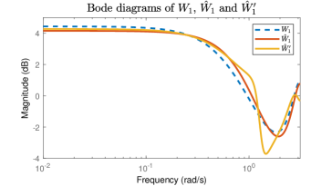
Figure 2: Bode diagrams of $W_{1}$, $\hat{W}_{1}$ and $\hat{W}_{1}^{\prime}$

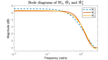
Figure 3: Bode diagrams of $W_{2}$, $\hat{W}_{2}$ and $\hat{W}_{2}^{\prime}$

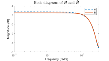
Figure 4: Bode diagrams of $H$, $\hat{H}$

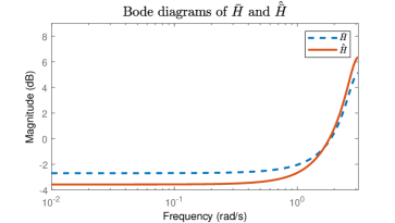
Figure 5: Bode diagrams of ${\bar{H}}$, $\hat{\bar{H}}$

Next we want to identify $F(z)$ and $K(z)$ in the feedback model. To this purpose we use the ARMAX identification algorithm described in subsection 3.1, referring to a model (17), with input $y_{2}$ and output $y_{1}$.
Since we do not know the true orders, we suppose

$$\begin{split}A(z^{-1})&=1+\sum\limits_{k=1}^{3}a_{k}z^{-k},\\ B(z^{-1})&=z^{-1}B_{1}(z^{-1})=z^{-1}(\sum\limits_{k=0}^{3}b_{k}z^{-k}),\\ C(z^{-1})&=1+\sum\limits_{k=1}^{3}c_{k}z^{-k}.\end{split}$$

Note that $A$ should have the same order as $C$, since we have assumed that $K=A^{-1}C$ is normalized at $\infty$. The estimation results are

$$\hat{F}=\frac{-0.02217z^{-1}-0.02322z^{-2}-0.3411z^{-3}+0.2154z^{-4}}{1+0.0009619z^{-1}+0.04707z^{-2}+0.02051z^{-3}},$$

$$\hat{K}=\frac{1+0.2588z^{-1}+0.4005z^{-2}+0.4596z^{-3}}{1+0.0009619z^{-1}+0.04707z^{-2}+0.02051z^{-3}}.$$

With these estimates we then calculate a corresponding estimate $\hat{W}^{\prime}_{1}$ of $W_{1}$ by the formula

$$\hat{W}^{\prime}_{1}=(1-\hat{F}\hat{H})^{-1}\hat{K}.$$

Its Bode graph is the orange line, compared with $W_{1}$ and $\hat{W}_{1}$ in Fig. 2. Since $\hat{W}_{1}$ has larger orders of both numerator and denominator than those of $W_{1}$, there is some overfitting and the Bode graph of $\hat{W}_{1}^{\prime}$ is not as smooth as those of $W_{1}$ and $\hat{W}_{1}$ in the high frequency range.

5.2 Example 2

In this subsection and in the next one we consider the identification of two-dimensional processes of rank 1 subjected to an external input $u$. We generate a scalar white noise $u$ independent of $e$ and identify a 2-dimensional process model (20) as described in the previous section 4.
In this example the true system is described by

$$\begin{split}F(z)&=z^{-1}\begin{bmatrix}0.3+0.7z^{-1}+0.3z^{-2}\\ 0.15+0.9z^{-1}-0.5z^{-2}\end{bmatrix},\\ K(z)&=\begin{bmatrix}\frac{1+0.1z^{-1}+0.4z^{-2}}{1+0.3z^{-1}+0.4z^{-2}}\\ \frac{1-0.1z^{-1}+0.4z^{-2}}{1-0.2z^{-1}+0.1z^{-2}}\end{bmatrix}\,.\end{split}$$ (23)

We use the same $F$ as in Van den Hof, Weerts, and Dankers (2017) (where it is called $G(q)$). But their $K$ is not normalized, so we use a different one. Both components of our $K(z)$ here are normalized and minimum-phase so the overall model is an innovation model.

From the model (23) we generate a two-dimensional time series of $N=500$ data points $\{\bar{y}_{i}(t);t=1,\ldots,N,\,i=1,2\}$. The simulation is run with $u$ and $e$ two independent scalar white noises of variances $2$ and $1$. Of course here we also measure the input time series $u$. First, we estimate $F(z)$ by fitting the deterministic relations

$$A_{i}(z^{-1})y_{i}(t)=B_{i}(z^{-1})u(t-1),\quad(i=1,2)$$

where we assume all with 3 unknown parameters,

$$\begin{split}A_{1}(z^{-1})=1+\sum_{k=1}^{3}{a}_{1,k}z^{-k},\quad A_{2}(z^{-1})=1+\sum_{k=1}^{3}{a}_{2,k}z^{-k}.\\ B_{1}(z^{-1})=z^{-1}\sum_{k=0}^{2}{b}_{1,k}z^{-k},\quad B_{2}(z^{-1})=z^{-1}\sum_{k=0}^{2}{b}_{2,k}z^{-k}.\end{split}$$

Applying a least square method we obtain

$$\begin{split}&y(t)-\tilde{y}(t)=\hat{F}u(t)\\ &=\begin{bmatrix}\frac{0.2901+0.7977z^{-1}+0.4339z^{-2}}{1+0.2137z^{-1}-0.02525z^{-2}-0.05393z^{-3}}\\ \frac{0.1302+0.9191z^{-1}-0.6492z^{-2}}{1-0.1363z^{-1}-0.1090z^{-2}-0.05338z^{-3}}\end{bmatrix}u(t-1).\end{split}$$

The corresponding Bode diagrams are shown in Fig. 6 and in Fig. 7.

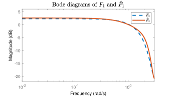
Figure 6: Bode diagrams of $F_{1}$ and $\hat{F}_{1}$ in example 2

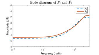
Figure 7: Bode diagrams of $F_{2}$ and $\hat{F}_{2}$ in example 2

Then we estimate $K(z)$ from (21) by the same procedure we used to estimate $W(z)$ in (22). Suppose

$$A_{i}(z^{-1})\tilde{y}(t)=B_{i}(z^{-1})e(t),\quad(i=1,2)$$

with (since $K$ is normalized)

$$\begin{split}A_{1}(z^{-1})=1+\sum_{k=1}^{3}{a}_{1,k}z^{-k},\quad A_{2}(z^{-1})=1+\sum_{k=1}^{3}{a}_{2,k}z^{-k}.\\ B_{1}(z^{-1})=1+\sum_{k=1}^{3}{b}_{1,k}z^{-k},\quad B_{2}(z^{-1})=1+\sum_{k=1}^{3}{b}_{2,k}z^{-k}.\end{split}$$

and obtain

$$\hat{K}(z)=\begin{bmatrix}\frac{1+0.4940z^{-1}+0.2391z^{-2}+0.1936z^{-3}}{1+0.7235z^{-1}+0.3215z^{-2}+0.07442z^{-3}}\\ \frac{1+0.5175z^{-1}+0.3272z^{-2}+0.03482z^{-3}}{1+0.4528z^{-1}-0.0283z^{-2}+0.07029z^{-3}}\end{bmatrix},$$

whose corresponding Bode diagrams are in Fig. 8 and Fig. 9. Here we obtain reasonable estimates of both $K_{1}$ and $K_{2}$.

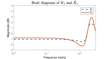
Figure 8: Bode diagrams of $K_{1}$ and $\hat{K}_{1}$ in example 2.

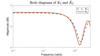
Figure 9: Bode diagrams of $K_{2}$ and $\hat{K}_{2}$ in example 2.

5.3 Example 3

Again, we generate a scalar white noise input $u$ independent of $e$ and identify a two-dimensional system (20), as in the previous subsection. The true system, is described by

$$\begin{split}F(z)&=z^{-1}\begin{bmatrix}1+0.3z^{-1}-0.1z^{-2}\\ 2-0.9z^{-1}+0.06z^{-2}\end{bmatrix},\\ K(z)&=\begin{bmatrix}\frac{1-0.9z^{-1}+0.2z^{-2}}{1+0.3z^{-1}+0.4z^{-2}}\\ \frac{1-0.1z^{-1}+0.4z^{-2}}{1-0.6z^{-1}+0.1z^{-2}}\end{bmatrix}.\end{split}$$

The simulation is run with $u$ and $e$ two independent scalar white noises of variances $2$ and $1$. We generate a two-dimensional time series of $N=500$ data points $\{\bar{y}_{i}(t);t=1,\ldots,N,\,i=1,2\}$, and suppose we also measure the input time series of $u$. Firstly, we estimate $F(z)$ by fitting the deterministic relation $y(t)=F(z)u(t)$ rewritten as

$$A_{i}(z^{-1})y_{i}(t)=B_{i}(z^{-1})u(t-1),\quad(i=1,2)$$

where the polynomials are chosen of degree 3, i.e.

$$\begin{split}A_{1}(z^{-1})&=1+\sum_{k=1}^{3}{a}_{1,k}z^{-k},\quad A_{2}(z^{-1})=1+\sum_{k=1}^{3}{a}_{2,k}z^{-k}.\\ B_{1}(z^{-1})&=\sum_{k=0}^{3}{b}_{1,k}z^{-k},\quad B_{2}(z^{-1})=\sum_{k=0}^{3}{b}_{2,k}z^{-k}.\end{split}$$

Applying a least square method we obtain

$$\begin{split}&y(t)-\tilde{y}(t)=\hat{F}u(t)\\ &=\begin{bmatrix}\frac{0.9807+1.353z^{-1}+1.114z^{-2}+0.5196z^{-3}}{1+1.064z^{-1}+0.903z^{-2}+0.3815z^{-3}}\\ \frac{1.991-1.831z^{-1}-0.09642z^{-2}+0.2789z^{-3}}{1-0.4595z^{-1}-0.2792z^{-2}+0.04673z^{-3}}\end{bmatrix}u(t-1).\end{split}$$

The corresponding Bode graphs are shown in Fig. 10 and Fig. 11. In Fig. 10, the Bode graph of $\hat{F}_{1}$ shows some overfitting since the order of $F$ is somewhat far from the true order (in fact $A_{1}=1$ with order $0$, but we suppose a degree of $3$. Assuming we know the orders of $A_{1}$, $B_{1}$, we get the estimate

$$\hat{F}_{1}^{\prime}=0.9802z^{-1}+0.314z^{-2}-0.09327z^{-3},$$

which is closer to $F_{1}$.

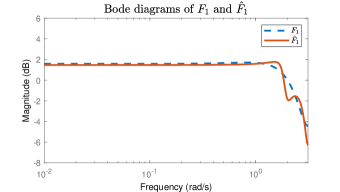
Figure 10: Bode diagrams of $F_{1}$ and $\hat{F}_{1}$ in example 3

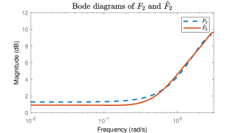
Figure 11: Bode diagrams of $F_{2}$ and $\hat{F}_{2}$ in example 3

Then we estimate $K(z)$ from (21) by the same procedure we used to estimate $W(z)$ in (22). Suppose

$$A_{i}(z^{-1})\tilde{y}(t)=B_{i}(z^{-1})e(t),\quad(i=1,2)$$

with (since $K$ is normalized)

$$\begin{split}A_{1}(z^{-1})=1+\sum_{k=1}^{3}{a}_{1,k}z^{-k},\quad A_{2}(z^{-1})=1+\sum_{k=1}^{3}{a}_{2,k}z^{-k}.\\ B_{1}(z^{-1})=1+\sum_{k=1}^{3}{b}_{1,k}z^{-k},\quad B_{2}(z^{-1})=1+\sum_{k=1}^{3}{b}_{2,k}z^{-k},\end{split}$$

obtaining

$$\hat{K}(z)=\begin{bmatrix}\frac{1-1.481z^{-1}+0.9142z^{-2}-0.2516z^{-3}}{1-0.2452z^{-1}+0.3701z^{-2}-0.1293z^{-3}}\\ \frac{1-0.8098z^{-1}+0.2342z^{-2}-0.2265z^{-3}}{1-1.28z^{-1}+0.2189z^{-2}+0.1462z^{-3}}\end{bmatrix},$$

the corresponding Bode diagrams are in Fig. 12 and Fig. 13.

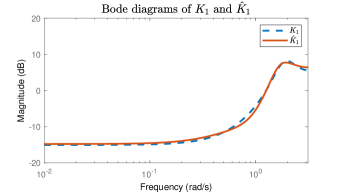
Figure 12: Bode diagrams of $K_{1}$ and $\hat{K}_{1}$ in example 3.

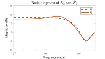
Figure 13: Bode diagrams of $K_{2}$ and $\hat{K}_{2}$ in example 3.

All the simulation examples show that the transfer functions of the rank-deficient structure can be identified from standard identification algorithms with rather good results. Of course, with a prior knowledge of the orders of the transfer functions, the identification results will be closer to the true functions.

6 Conclusions

We have shown that a rank-deficient process admits a special feedback structure with a deterministic feedback channel which can be used to split the identification in two steps, one of which can be based on standard PEM algorithms while the other is based on a deterministic least squares fit. Simulations show that standard identification algorithms can be easily applied to identify the transfer functions of this structure.

References

- Basu, Li, and Mochailidis (2019) Basu, S., Li, X., and Mochailidis, G. (2019). Low rank and structured modeling of high-dimensional vector autoregressions. IEEE Transactions on Singnal Processing, 67(5), 1207-1222.
- Cao, Lindquist, and Picci (2020) Cao, W., Lindquist, A., and Picci, G. (2020). Spectral rank, feedback, causality and the indirect method for CARMA identification. 59th IEEE Conference on Decision and Control (CDC), 4299-4305, Jeju, Korea (South).
- Deistler (2019) Deistler, M. (2019). Singular ARMA systems: A structural theory. Numerical Algebra, Control and Optimization, 9(3), 383-391.
- Deistler et al. (2010) Deistler, M., Anderson, B.D.O., Filler, A. and Chen, W. (2010). Generalized linear dynamic factor models: An approach via singular autoregressions. European Journal of Control, 16(3), 211-224.
- Georgiou and Lindquist (2019) Georgiou, T. T. and Lindquist, A. (2019). Dynamic relations in sampled processes. IEEE Control Systems Letters, 3(1), 144-149. Investigating causal relations by econometric models and cross-spectral methods. Econometrica, 37(3), 424-438. Multiple Time Series, pp. 61-64. John Wiley and Sons, New York.
- Lindquist and Picci (2015) Lindquist, A. and Picci, G. (2015). Linear stochastic systems: A Geometric Approach to Modeling, Estimation and Identification. Springer.
- Ljung (2002) Ljung, L. (2002). System identification: theory for the user. 2nd ed. Tsinghua University Press, Beijing.
- Schölkopf et al. (2012) Schölkopf, B., Janzing, D., Peters, J., Sgouritsa, E., Zhang, K. and Mooij, J. (2012). On Causal and Anticausal Learning. In Proceedings of the 29 th International Conference on Machine Learning, Edinburgh, Scotland, UK.
- Van den Hof, Weerts, and Dankers (2017) Van den Hof, P., Weerts, H., and Dankers, A. (2017). Prediction error identification with rank-reduced output noise. 2017 American Control Conference, 382-387. Seattle, USA.
- Weerts, Van den Hof, and Dankers (2018) Weerts, H.H., Van den Hof, P.M., and Dankers, A.G. (2018). Identifiability of linear dynamic networks. Automatica, 89, 247-258.