Driving Behavior Explanation with Multi-level Fusion

Abstract

In this era of active development of autonomous vehicles, it becomes crucial to provide driving systems with the capacity to explain their decisions. In this work, we focus on generating high-level driving explanations as the vehicle drives. We present BEEF, for BEhavior Explanation with Fusion, a deep architecture which explains the behavior of a trajectory prediction model. Supervised by annotations of human driving decisions justifications, BEEF learns to fuse features from multiple levels. Leveraging recent advances in the multi-modal fusion literature, BEEF is carefully designed to model the correlations between high-level decisions features and mid-level perceptual features. The flexibility and efficiency of our approach are validated with extensive experiments on the HDD and BDD-X datasets.

1 Introduction

Over the last decade, research communities have devoted lots of effort on making cars safer, reliable and intelligent. Vehicles are more and more able to understand their environment, plan motions and take appropriate decisions. However, reaching a perfect driving accuracy is not sufficient to allow for real-world deployment of self-driving vehicles. In such a safety-critical domain, providing human-understandable explanations is crucial as it can favor the adoption of self-driving systems [18, 11] by increasing users’ trust [41] and easing regulation and model validation [3, 32].

In this paper, we aim at explaining the decisions of a driving model to a human user, as the vehicle drives. This is grounded towards the long-term goal of building driving systems capable of communicating the underlying reasons behind their decisions. Specifying the requirements an “explanation” should meet is a non-trivial problem per se [13]. Visual saliency maps [30, 28, 8] constitute broadly accepted explanations for computer vision systems. They explain the network’s predictions by highlighting spatial locations in the image on which the network relied the most to take its decision [6, 16]. However, saliency maps usually need to be interpreted, and their purely visual nature may not be well suited for human-machine interactions. As an answer, natural language justifications have been used to explain self-driving decisions [18]. Related to this effort on explainability, recent works leverage visual recognition methods to find justifications of human drivers’ decisions [26, 21]. Most valuable explanations are introspective in that they depend on the actual driving system and on its inner processing that leads to the produced driving decisions [18]; this contrasts with post-hoc rationalizations that only consider the final driving decisions of the system [23, 35, 21].

On top of a simple self-driving backbone, we design an explanation module that produces introspective explanations by conditioning its reasoning on both the driving decisions and intermediate perceptual features of the driving system. This is motivated by the fact that final driving predictions hardly contain the necessary information to recover the precise cause for a decision, as various possible explanations collapse to the same behavior. For example, a car braking can be caused by multiple factors such as a red light, crossing pedestrians or a stop sign. The precise cause is lost through the processing as these different situations trigger the same braking behavior. We thus argue that features at different semantic levels need to be fused together: late features containing the system decisions, in the form of the predicted trajectory, and intermediate spatio-temporal features containing perceptual scene information. A fusion problem thus emerges to aggregate information from these multi-level features. In that respect, we leverage the recent literature on multi-modal fusion techniques for Visual Question Answering (VQA) systems [4, 5] that we adapt to our needs.

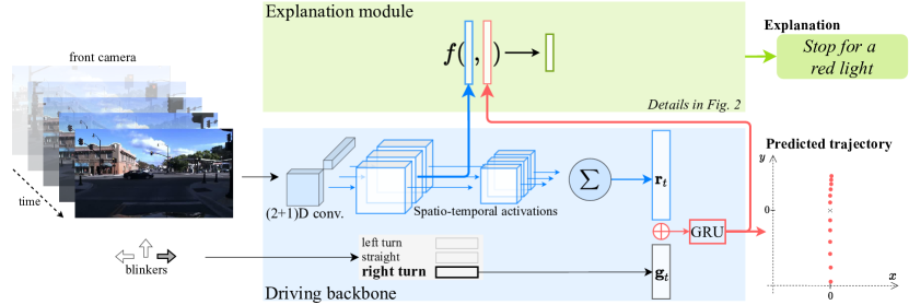
Figure 1: Model overview. The architecture is composed of an explanation module (green box) on top of a self-driving backbone (blue box). The driving system takes both the camera stream and the blinker state as input to predict the future trajectory of the car from a bird-eye view. Simultaneously, the explanation module produces a justification for the driving decision by jointly processing the high-level driving decision and intermediate perceptual features extracted from the driving system.

Our design choices are validated on two datasets, in different settings, thus showing the generic aspect of our approach. First, on the Honda Deep Drive (HDD) dataset [26], which associates each video frame to a cause label, explanations in the form of cause labels are produced as the system drives, i.e. in an online fashion. Second, with the Berkely Deep Drive eXplanation (BDD-X) dataset [18], explanations take the form of natural language justifications, generated in an offline fashion.

The contribution is three-fold: (1) we equip self-driving systems with a module providing introspective explanations, (2) we draw a comparison with VQA systems and adapt the BLOCK module to fuse high-level driving decisions with intermediate perceptual features, and (3) we exhibit the versatility of our approach with experiments in various settings (online/offline, classification/generation).

2 Architecture overview

In this section, we present BEEF, a module providing explanations for a driving system’s decision, as illustrated in Figure 1. Explanations are provided in an online fashion as only the current and previous inputs are used. The central design choice of BEEF is that decisions are explained by analyzing the correlations between mid-level perception and high-level decision signals. This corresponds to introspective explanations as the network accesses the driving backbone’s internal representations. The architecture’s backbone is presented in Section 2.1, and the explanation module in Section 2.2.

2.1 Driving backbone

As in previous work [2, 31, 40, 20, 27], the driving system is a vision-based end-to-mid trajectory prediction model: at each timestep $t$, our backbone network predicts the future positions the ego-vehicle should reach. It takes as input the current frame $\mathcal{I}_{t}$ and the $T$ previous frames $\mathcal{C}_{t}=[\mathcal{I}_{t-T},...,\mathcal{I}_{t-1}]$ of the front camera. These $(T+1)$ color images are stacked to form $\mathcal{X}_{t}=[\mathcal{I}_{t-T},...,\mathcal{I}_{t-1},\mathcal{I}_{t}]$, represented at the left of Figure 1. We pass this input tensor to a 3D Convolutional Neural Network to obtain $\mathbf{r}_{t}=\operatorname{3DCNN}\left(\mathcal{X}_{t}\right)\in\mathbb{R}^{d}$, the vector representing the input image sequence $\mathcal{X}_{t}$. Note that our setting is generic enough to be used with any driving architecture instead of our $\operatorname{3DCNN}$, provided that intermediate representations can be accessed. Here, we experimented with an R(2+1)D network [33]. It processes input data through a series of five residual convolutional blocks, where 3D convolution kernels are factorized into separate spatial and temporal components.

To predict the future trajectory of the vehicle, the model needs to be informed about high-level goals of the car. We represent the input goal as a categorical variable $g_{t}\in\left\{\textit{left},\textit{straight},\textit{right}\right\}$ that indicates the state of the car turn signals, as in previous works [10]. The goal $g_{t}$ is then associated to a vector $\mathbf{g}_{t}$ of trainable parameters through an embedding table, shown in the bottom of Figure 1.

In our framework, the future vehicle positions are generated by a recurrent model, here a $\operatorname{GRU}$ network [9], similarly to previous work [20]. At every time step $t$, $K$ future positions are predicted by the driving system: for each decoding step $k\in\{1\dots K\}$, the network takes the same representation $\left[\mathbf{r}_{t}\oplus\mathbf{g}_{t}\right]$ as input and updates its internal state $\mathbf{h}_{k}$ to predict a future position $(\hat{x}_{t,k},\hat{y}_{t,k})$:

$$\big{(}\left(\hat{x}_{t,k},\hat{y}_{t,k}\right),\mathbf{h}_{k}\big{)}=\operatorname{GRU}\left(\left[\mathbf{r}_{t}\oplus\mathbf{g}_{t}\right],\mathbf{h}_{k-1}\right),$$ (1)

where $\oplus$ designates the concatenation operator.

The first internal state $\mathbf{h}_{0}$ is initialized with the null vector. The driving backbone is trained under the imitation learning paradigm with a mean squared error regression objective $\mathcal{L}_{\textit{drive}}$. As we see in Section 3.2.1, this end-to-mid architecture can be modified to fit into the end-to-end setting. To do so, we replace the recurrent prediction head by a regression, trained to directly fit the vehicle controls.

2.2 Explanation module

As humans cannot reasonably decipher and interpret the driving system’s inner processing, we build an explanation module to justify the driving decisions. This module is designed to reason about internal representations of the driving backbone, under the light of the driving decision. Indeed, to explain why a specific trajectory was output by the driver, we posit that merging intermediate spatio-temporal perceptual features with the higher-level decision features is key. As exemplified in the introduction, various causes may collapse to produce a same output: a car braking could be caused by multiple events such as a red light, the presence of a pedestrian or a stop sign. Hence, for the system to accurately recognize that the vehicle stops because of a red light, it should be given the information that the ego-vehicle chose to stop (decision), but also that there is a red light (perception).

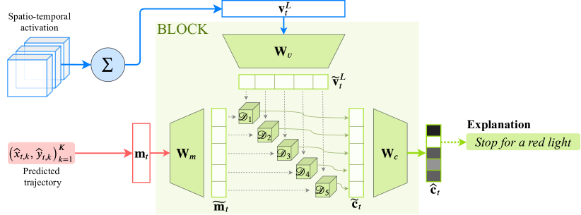
Figure 2: Explanation module. The structure of BLOCK bilinear fusion enables to find relevant correlations between a perceptual mid-level representation $\mathbf{v}_{t}^{L}$ and high-level decision features $\mathbf{m}_{t}$. This forms $\mathbf{\hat{c}}_{t}$ which scores each possible explanation.

2.2.1 Overview

For a given residual block $L$ of the $\operatorname{3DCNN}$, we extract spatio-temporal activation maps $\mathcal{V}_{t}^{L}\in\mathbb{R}^{t_{L}\times h_{L}\times w_{L}\times d_{L}}$, which contain localized information about the input frame sequence. We aggregate all this information using a space-time average pooling to obtain $\mathbf{v}_{t}^{L}$; this vector contains intermediate perceptual features. Besides, we define the vector $\mathbf{m}_{t}~{}=~{}\left[\hat{x}_{t,1},\hat{y}_{t,1},...,\hat{x}_{t,K},\hat{y}_{t,K}\right]$, the flattened vector coordinates of all future positions predicted by the recurrent network. Both the decision vector $\mathbf{m}_{t}$ and the perceptual features $\mathbf{v}_{t}^{L}$ are fused together with a function $f$ to form $\mathbf{\hat{c}}_{t}=f(\mathbf{m}_{t},\mathbf{v}_{t}^{L})$, where $\mathbf{\hat{c}}_{t}\in\mathbb{R}^{d_{c}}$ is the predicted probability distribution over each of the $d_{c}$ candidate causes.

We now discuss the instantiation of the fusion operation $f$. Its design is not trivial as it merges information from vectors of a very different nature: $\mathbf{v}_{t}^{L}$ contains perceptual features extracted from a deep network and $\mathbf{m}_{t}$ is a list of 2D coordinates. We thus leverage the family of bilinear models for multi-modal fusion [4, 17, 39, 5] as these fusion techniques have proven to be effective in contexts with heterogeneous media as for Visual Question Answering. In their general form, bilinear models are parameterized by a tensor of trainable weights $\mathcal{T}\in\mathbb{R}^{2K\times d_{L}\times d_{c}}$, and defined by:

$$\mathbf{\hat{c}}_{t}=\mathcal{T}\times_{1}\mathbf{m}_{t}\times_{2}\mathbf{v}_{t}^{L},$$ (2)

where $\times_{i}$ refers to the mode-$i$ product. In other terms, each output dimension can be written as $\mathbf{\hat{c}}_{t}[i]~{}=~{}\mathbf{m}_{t}^{\top}~{}\mathcal{T}_{i}~{}\mathbf{v}_{t}^{L}$, where $\mathcal{T}_{i}~{}\in~{}\mathbb{R}^{2K\times d_{L}}$ is the $i$-th slice of $\mathcal{T}$.

As we need to model rich correlations between mid- and top-level features of the network, we use the BLOCK fusion [5], a recent and efficient bilinear variant, where $\mathcal{T}$ is factorized by constraining the block-term ranks of the tensor. Formally, this model specifies a structure on $\mathcal{T}$ such that Equation 2 can be expressed a sequence of light operations, as illustrated in Figure 2:

$$\mathbf{\tilde{m}}_{t} =\mathbf{W}_{m}\mathbf{m}_{t},\hskip 2.84544pt\quad\quad\quad\quad\quad\mathbf{\tilde{v}}_{t}^{L}=\mathbf{W}_{v}\mathbf{v}_{t}^{L}$$ (3)

$$\mathbf{\tilde{c}}_{t} =\mathcal{D}\times_{1}\mathbf{\tilde{m}}_{t}\times_{2}\mathbf{\tilde{v}}_{t}^{L},\quad\quad\mathbf{\hat{c}}_{t}=\mathbf{W}_{c}\mathbf{\tilde{c}}_{t},$$ (4)

where $\mathcal{D}$ is a block-diagonal tensor.

Finally, the output vector is transformed into a probability distribution $\mathbf{p}_{t}$ over possible classes using the softmax operator: $\mathbf{p}_{t}=\mathrm{softmax}(\mathbf{\hat{c}}_{t})$. In Section 3.2.1, we extend this classification setup to generate natural language explanations, by using a language model instead of the classification layer.

2.2.2 Learning

Training the explanation module is in itself a challenge. To meet the standard supervised learning setting, ground-truth explanations for the driving system are needed. In other words, the training algorithm should be given annotations about why this specific driving model is taking its decision. As we do not have access to this type of annotations, we make the following hypothesis: when a self-driving system is trained to mimic a human driver, explanations for the neural network’s decisions coincide with justifications of the human driver. This assumption allows us to leverage human driver justifications as a proxy to ground-truth explanations of the driving model.

Recent work of [26, 21] propose to recognize action justifications (such as “stop for red light” or “deviate for parked car”) in driving videos. While they tackle the task of identifying causes of driving behaviors, these works are different from ours as they do not involve any driving model. From a practical point-of-view, this means that when predicting a cause, we never use input images directly and we only allow ourselves to look at internal representations of a driving backbone.

Under the supervision of the ground-truth cause $c$, the explanation module is optimized with:

$$\mathcal{L}_{\textit{explain}}=-\frac{1}{T}{\textstyle\sum}_{t=1}^{T}\log\mathbf{p}_{t}[c].$$ (5)

Objectives $\mathcal{L}_{\textit{drive}}$ and $\mathcal{L}_{\textit{explain}}$ are linearly combined and jointly optimized.

2.3 Link with Visual Question Answering (VQA)

The BLOCK fusion employed here was originally designed for VQA systems, where the representations of the question and the image are fused together to output the correct answer. VQA systems require ways to model interactions between feature vectors. Some work perform this multi-modal fusion using bilinear models, which are made tractable by sampling methods like MCB [12] or through tensor factorization such as MUTAN [4], MLB [17], MFB [39] or BLOCK [5]. In other work of [25], the FiLM layer is designed to perform fusion by linearly modulating visual features, conditioned on language vectors. Even if these fusion techniques were originally developed for VQA, many other applications benefit from those methods. Indeed, fusing multiple representations in deep learning architectures has drawn interest in visual relationship detection [5], image generation with StyleGAN [15] or conditional domain adaptation [22].

We can draw a parallel between fusion-based VQA systems and our explanation module. In our case, a question in the form of a trajectory is asked, and the explanation module builds the answer from the driving backbone’s representations. More generally, our work illustrates the power of tensor-based methods to model fine-grained correlations between heterogeneous high-dimensional features.

3 Experiments

We validate the design of BEEF in Section 3.1. In Section 3.2, we show that BEEF can be adapted to different settings, with an extension to offline natural language explanations.

3.1 Online introspective explanations

This section presents an experimental study of the explanation module presented in Section 2. We evaluate the quality of the explanations provided by BEEF with respect to previous action recognition works. The design of the explanation module is validated and we show (1) the effectiveness of using both perceptual and high-level features, and, (2) the relevance of employing a BLOCK fusion.

Table 1: Comparison to state-of-the-art on the cause labels of HDD. Results in bold are the best among online models. For the sake of completeness, we also report performance of offline models.

		Individual causes
System	Online/ Offline	Congest.	Sign	Red light	Crossing vehicle	Parked vehicle	Crossing pedestrian	Overall mAP	Driver MSE
		Action recognition (no driver)
CNN+Sens. [26]	On.	39.72	46.83	45.31	—	7.24	2.15	28.25	$\times$
I3D [21]	Off.	64.8	71.7	63.6	21.5	15.8	26.2	43.9	$\times$
I3D+GCN [21]	Off.	74.1	72.4	76.3	26.9	20.4	29.0	49.9	$\times$
		Driver only (no explanation)
Driver	On.	$\times$	$\times$	$\times$	$\times$	$\times$	$\times$	$\times$	1.33
		Introspective explanation
Multi-head	On.	81.25	66.59	75.46	31.21	10.24	25.62	48.39	1.36
BEEF	On.	80.38	63.41	81.94	41.19	12.18	27.19	50.96	1.33

3.1.1 HDD dataset [26]

To study driving behavior causes from a driver-centric view, the Honda Deep Drive (HDD) dataset has been introduced [26]. The dataset gathers 137 driving sessions recorded in the San-Francisco Bay Area. In total, 104 hours of human driving videos have been acquired, synchronized with CAN bus signals and GPS/IMU information. We only use front camera images, turn signals and GPS positions to train our model. Additionally to these signals, several layers of frame-level annotations are provided to describe the driving behavior. Among these layers, we focus on the cause labels which convey information about the underlying reason explaining the driver’s behavior (e.g. “stop for red light” or “deviate for parked car”). Following the literature on action detection [29, 26], we evaluate each frame independently and we report the value of the mean Average Precision (mAP).

3.1.2 State-of-the-art comparison

As stated in the introduction, our work is the first driving system equipped with an introspective explanation module. Previous works using HDD would perform driving scene recognition, mainly on goal-oriented labels. Even if some of them are trained on the cause labels, which explain the behavior of the human driver, they adopt a setup of action recognition and do not consider any driving model. To measure the relevance of our online introspective explanations, we compare against state-of-the-art methods for action recognition:

• CNN+Sensors [26] where convolutional features and sensor values are merged before being passed to an LSTM that models temporal dependencies;

• I3D [7], a fined-tuned I3D network implemented by [21];

• I3D+GCN [21] where the scene is analyzed by multiple perception models that infer depth, detect objects and segment the relevant areas. This information is processed by multiple graph convolution networks in order to recognize the cause label.

Importantly, I3D+GCN [21] is an offline model as causes are predicted using previous and future frames. Besides, we also evaluate an internal baseline, named Multi-head, which simply adds an auxiliary branch to the last layer of the $\operatorname{3DCNN}$ without using the predicted trajectory, nor any fusion. Also, we note Driver the backbone driving system, i.e. without the explanation module.

Results of this comparison are reported in Table 1. First, we observe that BEEF outperforms all action recognition systems, including offline ones. While the average performance of BEEF is indeed higher than I3D+GCN, we notice a slight performance drop on some classes (e.g. Sign, Parked vehicle). We hypothesize that this stems from the fact that annotations from these classes have a shorter time-span. This may benefit offline models which can access future frames, while these frames remain not accessible for BEEF. This is supported by the value $\rho=0.71$ of the Spearman correlation between the average duration of annotations from each class and the relative performance shift. Overall, despite a slight drop in some classes, the online architecture of BEEF is suitable for real-world self-driving explanations, unlike the offline action recognition model of [21].

Besides, we see that BEEF performs better than the Multi-head baseline, for which the explanation module only uses perceptual features. This shows their complementarity with the predicted trajectory and stresses the importance of combining them together to provide explanations. We note that by fusing the predicted trajectory with the perceptual features in BEEF, the cause prediction may be indirectly influenced by the blinker signal used in the driving system. To make sure that this does not solely explain the gain in predictive performance, we also evaluate a modified Multi-head model which uses the blinker information by concatenating $\mathbf{g}_{t}$ with the output of the $\operatorname{3DCNN}$. This variant obtains an overall mAP of 49.98, a higher score than the original Multi-head but still below BEEF. This emphasizes the importance of the fusion module used in BEEF, as both Multi-head architectures struggle to balance between driving and explanation objectives.

3.1.3 Choice of the layer $L$

BEEF fuses the high-level decision vector $\mathbf{m}_{t}$ with low-level perception features $\mathbf{v}_{t}^{L}$. Here, we study how the performance of BEEF depends on the chosen perception layer. Figure 4 shows the overall mAP cause prediction performances with respect to the layer used for the perceptual features in BEEF. The horizontal dotted line corresponds to the Multi-head baseline shown in Table 1.

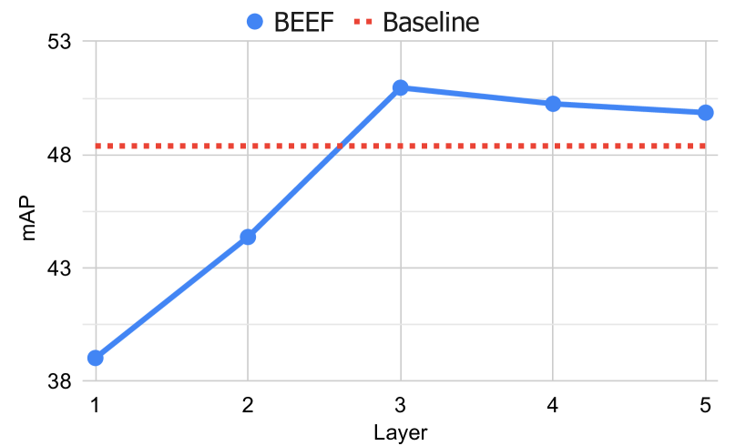
Figure 3: BEEF performance by layer.

Fusion model	mAP	Driver MSE
Layer 3	45.39	1.38
Cat+MLP	46.64	1.38
MFB	39.10	1.43
MLB	38.59	1.37
MUTAN	45.80	1.40
Bilinear	49.82	1.42
BLOCK	50.96	1.33

Figure 4: Fusion comparison. Fusions are performed between driving decisions $\mathbf{m}_{t}$ and mid-level features $\mathbf{v}_{t}^{3}$.

Unsurprisingly, we observe that early layers poorly perform compared to the multi-head baseline. Early features of the network are too low-level to recognize relevant visual patterns for the cause identification. We observe a performance peak at the third layer. At this level, the representation contains rich perceptual signals, but still conveys enough cause information that is complementary to the final decision. As we use higher-level features of the network, we move away from the balance in the trade-off between representation richness and independence to the decision. In other words, the explanation module is fed with two vectors that convey similar information, which makes their combination less useful. Interestingly, we remark that BEEF with layer 5 is better than the multi-head baseline: there is still information to extract from the interaction between the predicted trajectory and the hidden layers of the network. This validates the design of the explanation module as a fusion between mid-level representations and high-level driving decisions.

3.1.4 Fusion comparison

The design of the fusion operation used in the explanation module is a critical element of the architecture. To take advantage of the complementarity between both inputs, the fusion operator must allow fine-grain correlations. The experiment shown in Table 4, compares the BLOCK fusion with other techniques, including:

• Cat+MLP concatenates decision and mid-level features followed by a 2-layer perceptron,

• MLB, MFB and MUTAN are bilinear fusion methods developed for VQA [17, 39, 4],

• Bilinear is the unstructured bilinear model that follows Equation 2.

Moreover, we compare to a multi-head model with a 2-layer perceptron connected at layer 3, without any fusion. This model is referred to as Layer 3.

Using only Layer 3 performs poorly, which again supports the fact that driving decisions are important inputs for the explanation module. Among all the compared fusions, BLOCK provides the most relevant explanations. It shows that this bilinear model is able, through its structure, to find the correlations between its inputs that carry relevant information for its task. Interestingly, BLOCK is the only fusion model that does not degrade the driving performance, while unstructured bilinear models heavily degrade the driving capacity. As this model does not involve mono-modal projections, it lacks flexibility and forces the trajectory prediction to adapt to the explanation task.

3.2 Offline natural language explanations

Towards the long-term goal of developing human-vehicle dialogs, we aim at building a driving system that formulates explanations in natural language. We are motivated by the fact that open-domain sentences can convey finer and richer semantics than predefined classes. In this subsection, the cause classification becomes a language generation problem and we adapt the explanation module to enable the generation of textual explanations. To learn and evaluate our model, we use the recent BDD-X dataset [18], which provides natural language explanations for human driving sessions.

Task	Model	BLEU-4		METEOR		CIDEr-D
Action recognition (no driver)	“because the light is red”	5.85		10.74		59.50
	Vid-to-Text [36]	6.33		11.19		53.35
Rationalization (offline)	Rationalization [18]	6.52		12.04		61.99
	Decision Features	9.15	$\pm{}$.37	14.34	$\pm{}$.23	92.08	$\pm{}$1.3
Introspective explanation (offline)	SAA [18]	7.07		12.23		66.09
	WAA [18]	7.28		12.24		69.52
	Layer 2	7.96		13.51		83.46
	BEEF	9.81	$\pm{}$.32	14.79	$\pm{}$.22	97.31	$\pm{}$2.3

Table 2: Offline explanations generation on BDD-X. Values are given in percentages, standard deviations are computed on three runs with different seeds. The first line corresponds to a baseline that always generates the same sentence. Results of the Vid-to-Text model are reported from [18].

BDD-X dataset [18]

This dataset builds upon the BDDV dataset [37] by adding explanations to the driving sessions. The dataset is composed of $6\,984$ videos, each lasting about 40 seconds and containing about 3.8 annotations on average. The dataset totals 77 video hours and 26K annotations. Sensor data come from the front camera, GPS and IMU signals. In every driving session, open-domain natural language explanations are provided for each segmented sub-sequence.

3.2.1 Tailoring BEEF to the new setting

To fairly compare our approach with previous work on BDD-X [18], we need to make three modifications to the architecture presented in Section 2.

Natural language.     We adapt the explanation module to enable the generation of natural language justifications, instead of explanation labels. In practice, we replace the classification layer by an autoregressive model instantiated with an attention-based LSTM network [14] as done in [18].

End-to-end backbone.     We change the driving module to be end-to-end, instead of end-to-mid as presented in Section 2. In practice, the future trajectory prediction problem is simply replaced by a control command regression problem, and a single projection layer is used to output the acceleration and change of course values as in [18]. As a consequence, we slightly change the source of high-level decision features in BEEF. We use the last layer, i.e. layer 5, instead of the predicted trajectory as done in Section 2. Indeed, contrary to end-to-mid models, end-to-end models output a weak signal about the future vehicle position by solely predicting the current acceleration and steering values.

Offline explanations.     We conduct the learning and evaluation phases in an offline fashion as annotations are provided at the level of segmented driving sub-sequences. We straightforwardly adapt BEEF to the offline setting, by simply feeding the whole sequence as input and by generating a single justification for this sequence, as previously done on BDD-X [18].

Extracted frame
HL	because traffic is moving now	since the cars in front aren’t moving	since the car is free to move right
T=0	because the light is green and traffic is moving	because the car in front has stopped	because the car is turning to the right
T=0.3	as the light turns green and traffic is moving	because the light is red	because the car is entering another street
T=0.3	because the light is green and traffic is moving	as traffic ahead is stopped at a red light	to enter another road
T=0.3	because the light turns green	because traffic is stopped at a red light	because the road is clear of traffic

Table 3: Samples of generated explanations. HL stands for the Human gold Label. Other lines are generated by BEEF, with different runs obtained with various decoding temperature T: T=0 corresponds to the greedy decoding and lines with T=0.3 correspond to random decoding with T=0.3.

3.2.2 Competition, baselines and evaluation

BEEF is compared against previous models on the BDD-X dataset. This includes: (1) a deep video-captioning model that does not involve any driver: Vid-to-Text [36], (2) an offline rationalization model, namely the Rationalization baseline of [18], and, (3) offline introspective explanation models, namely SAA and WAA [18], which constrain the attention of the explainer to align with the attention of the driving system either strongly or weakly respectively for SAA and WAA. Moreover, as BEEF fuses intermediate features from Layer 2 with the Decision features of the last layer, we also evaluate against the two baselines considering these feature vectors independently.

Similarly to previous work [18], explanations are decoded in a greedy fashion and their quality is measured with the BLEU-4 [24], METEOR [1] and CIDEr-D [34] metrics.

3.2.3 Results analysis

Table 2 reports that BEEF obtains leading results on BDD-X by surpassing performances of previous works, namely Vid-to-Text, SAA and WAA, by a large margin on all of the evaluation metrics. Importantly, BEEF surpasses both the Layer 2 and Decision Features baselines: this is in line with results on HDD presented in Section 3.1.2 and it supports the claim that perceptual features (e.g. Layer 2) and high-level decision features are complementary for introspective explanations; moreover, it shows the flexibility and adaptability of our approach to various settings whether end-to-mid or end-to-end, online or offline, cause classes or textual justifications.

Finally, we show some qualitative samples of explanations generated by BEEF in Table 3, where the diversity of generated sentences is controled by tuning the temperature parameter of the decoding softmax. We observe reasonable and diverse explanations for various situations. In particular, we note that the different justifications decoded with a temperature T=0.3 are consistent with one another and remark that obtained explanations are diverse in two ways: syntactically and with respect to their completeness level as explanations can be more or less exhaustive when multiple explanations are simultaneously valid (e.g. the car stops for both a red light and stopped traffic). However, we empirically notice that when the decoding temperature is increased further (beyond 0.3), generated sentences start being semantically undermined. Increasing completeness and syntactic diversity without impairing the underlying semantics constitutes an exciting future research direction.

4 Conclusion

In this paper, we presented BEEF, an architecture that provides explanations for the decisions taken by a driving system. On top of a driving backbone, BEEF produces introspective explanations by fusing together high-level decisions and intermediate perceptual features. We showed that the BLOCK operator, originally developed to fuse multi-modal inputs, can be efficiently leveraged to fuse multi-level inputs. Our approach is validated on huge real-world driving datasets, HDD and BDD-X, where the quality of explanations surpasses previous state of the art. Besides, we showed the flexibility of BEEF to various settings (online/offline, cause classes/natural language justifications).

From a higher perspective, we advocate for more transparent and interpretable driving systems. In the future, we want to investigate the possibility of generating natural language explanations in an online fashion, thus moving towards explanation-centric human-machine dialog.

5 Supplementary material

5.1 Details and additional results on the HDD dataset

5.1.1 Implementation details

Following previous work with HDD [26, 38, 21], we sample the videos at 3 Hz. Each frame is resized to $90\times 160$ and concatenated with its $T=20$ previous frames to form a $(T+1)\times 3\times 90\times 160$ tensor. This sequence of images is passed as the input of a R(2+1)D convolutional neural network [33], pretrained on Kinetics [7]. The driver is trained to predict the trajectory of the vehicle in the next 2 seconds. The scale of trajectories is in meters. Besides, we found that we can increase driving performance by also learning to predict the positions two seconds in the past, in addition to the two seconds in the future. Thus, at every time step, we predict in total $K=13$ positions, corresponding to the local trajectory with 2 seconds horizon, at 3 Hz. As no official validation split is provided for HDD, we validate our hyper-parameters on 10% of the official training set that was kept aside training. The validation split that we used will be released along with our code. The explanation module BEEF merges the predicted trajectory with the internal driver representation, extracted at layer $L=3$, using a BLOCK fusion with a projection dimension of 256 and a core tensor composed of 5 blocks. Once validated, we train our models on the full training set for 70K iterations and report the results on the official test split, similarly to [21]. As $\mathcal{L}_{\textit{drive}}$ and $\mathcal{L}_{\textit{explain}}$ are differentiable with respect of the parameters of the system, they are jointly optimized with ADAM [19] with a learning rate of $1.0\times 10^{-4}$ and a batch size of $12$. The hidden dimension of the GRU to decode the trajectory is 256. Weights are initialized with a Xavier initialization. Random seeds for initialization and optimization are fixed at the beginning of each training for reproducibility, and will be given in our code repository. All our models are developed using PyTorch 1.3, and trained on a single Nvidia GeForce RTX 2080 Ti with 11Go of RAM.

5.1.2 Visualizations

Figure 5 presents qualitative visualization of the output of BEEF on test driving sessions of HDD. In addition, we provide additional video visualizations of BEEF performances on HDD in the companion zipped folder.

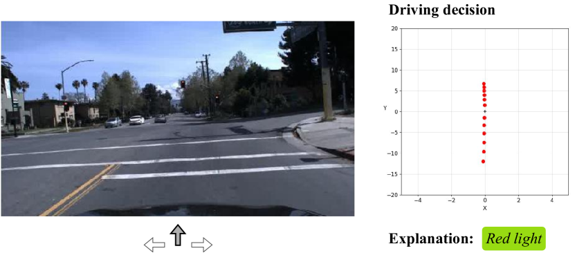
(a) Example of a car stopping for a red light.

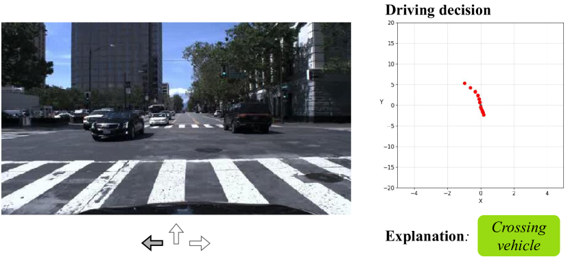
(b) Example showing the importance of the high-level driver intent (blinker) to predict the future trajectory.

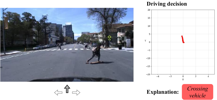
(c) Example of a failure case where the person on the skateboard is identified as a crossing vehicle.

Figure 5: Qualitative visualization of BEEF predictions on the HDD dataset. Arrows under each camera image represent the blinker’s state. For clarity’s sake, only the image at time $t$ is shown here.

5.2 Details and additional results on the BDD-X dataset

5.2.1 Implementation details

We follow the same data preprocessing and experimental protocol as the previous work on BDD-X [18]. In particular, we filter out explanations longer than 20 words from the training set and images are rescaled to $90\times 160\times 3$. The driving backbone is pretrained at 10 Hz and the explanation module attends over features of 20 frames equally spaced throughout the sequence. Hyper-parameters were found on the provided validation set: batch size is 32, the learning rate of the ADAM optimizer [19] is $3\times 10^{-4}$, the hidden dimension of the LSTM is 64, and layer 2 is used in the BLOCK fusion along with the decision features. Our pretrained driver has 0.43 and 9.11 Mean Absolute Error (MAE) for acceleration and course values respectively. Training a model takes about 10 hours on an NVIDIA 2080Ti.

5.2.2 Additional samples

Table 4 shows generated explanations (with a greedy decoding) on seven randomly chosen videos of the test set. After a manual verification, we observe that 29 out of the 34 explanations correspond to the driving sequence and correctly explain the driving behavior. Inspecting failures shows that they occur either by hallucinating street furniture (a stop light or a green light) or by interpreting the traffic as slowing down while there is no traffic (in one case).

In addition, we provide additional video visualizations of BEEF performances on BDD-X in the companion zipped folder.

Table 4: Explanations generated on BDD-X driving videos. These videos come from the test set and are not “cherry-picked”. Explanations are generated by the BEEF model and colors indicate whether the explanation matches the content of the video (green) or not (red), according to manual inspection. BLEU-4 and METEOR metrics are abbreviated to B4 and M respectively.

	Human (gold-label)	Generated by BEEF (greedy decoding)	B4	M
1	since there are many obstacles to be aware of	because traffic is moving at a steady speed	0	0
2	since the light ahead became red	because the light turned green	0	18.4
3	since the light is red and there are people crossing the road	because the light is red	16.5	1.4
4	because the lights are green and there is little traffic	because the road is clear	0	17.2
5	because the traffic ahead starts moving faster	because traffic is moving forward	0	19.9
6	because there are no nearby cars in its lane and the light is green	because the road is clear	0	12.5
7	as it prepares to make a left hand turn	because there is a stop sign	0	2.2
8	to enter another road while the light is green	because the road is clear	0	15.2
9	because there are no nearby cars in its lane impeding it	because the road is clear	0	5.9
10	for the red light and a pedestrian in the crosswalk	because the light ahead is red	0	16.1
11	for the red light	because the light is red	0	33.1
12	because there are cars and people nearby	because traffic is moving at a steady speed	0	8.7
13	because the car can turn right	because the road is clear	0	15.2
14	to avoid the car in front on the left	because the road is clear	0	2.5
15	because there are pedestrians blocking the path to the right	because there is a stop sign	0	23.2
16	since it is waiting for the pedestrians to cross	because there is a stop sign	0	3.5
17	because the pedestrians had moved out of the way	because the road is clear	0	16.9
18	since the car had just turned right	because the road is clear	0	4
19	because traffic is now moving in both lanes	because traffic is moving forward	0	25.2
20	because traffic is moving forward	because the car in front is slowing down	0	11.6
21	because traffic is moving faster in that lane	because the lane is clear	0	16.5
22	because now that lane is moving faster	because the car in front is slowing down	0	9.3
23	because traffic is moving slowly	because traffic is moving at a steady speed	34.6	39.7
24	because the cars ahead have stopped	because the light is red	0	14.1
25	because the van in front was’nt moving	because traffic is stopped	0	7.1
26	since the van started moving	because traffic is moving slowly	0	14.1
27	because the van stopped moving	because traffic is stopped	0	27.2
28	because the van in front is moving at different speeds	because traffic is moving slowly	0	15.1
29	as traffic in front of it moves slowly and merges together	because the car in front of it is moving forward	23.8	14.5
30	when traffic in front of it stops	because the car in front of it is stopped	29.9	24.1
31	as traffic in front of it moves forward slightly	because the car in front of it has stopped	29.9	17.5
32	because there are no nearby cars in its lane	because the car in front of it has slowed down	0	15.7
33	while there is a gap in traffic	because the car in front is moving forward	0	5.9
34	because there are no nearby cars in front of it	because the car in front is moving forward at a normal speed	0	22.8

References

- Banerjee and Lavie [2005] S. Banerjee and A. Lavie. METEOR: an automatic metric for MT evaluation with improved correlation with human judgments. In Proceedings of the Workshop on Intrinsic and Extrinsic Evaluation Measures for Machine Translation and/or Summarization@ACL 2005, Ann Arbor, Michigan, USA, June 29, 2005, pages 65–72, 2005. URL https://www.aclweb.org/anthology/W05-0909/.
- Bansal et al. [2019] M. Bansal, A. Krizhevsky, and A. S. Ogale. Chauffeurnet: Learning to drive by imitating the best and synthesizing the worst. In Robotics: Science and Systems XV, University of Freiburg, Freiburg im Breisgau, Germany, June 22-26, 2019, 2019. doi: 10.15607/RSS.2019.XV.031. URL https://doi.org/10.15607/RSS.2019.XV.031.
- Beaudouin et al. [2020] V. Beaudouin, I. Bloch, D. Bounie, S. Clémençon, F. d’Alché-Buc, J. Eagan, W. Maxwell, P. Mozharovskyi, and J. Parekh. Flexible and context-specific AI explainability: A multidisciplinary approach. CoRR, abs/2003.07703, 2020. URL https://arxiv.org/abs/2003.07703.
- Ben-Younes et al. [2017] H. Ben-Younes, R. Cadène, N. Thome, and M. Cord. Mutan: Multimodal tucker fusion for visual question answering. ICCV, 2017. URL http://arxiv.org/abs/1705.06676.
- Ben-Younes et al. [2019] H. Ben-Younes, R. Cadene, N. Thome, and M. Cord. Block: Bilinear superdiagonal fusion for visual question answering and visual relationship detection. In Proceedings of the AAAI Conference on Artificial Intelligence, volume 33, pages 8102–8109, 2019.
- Bojarski et al. [2017] M. Bojarski, P. Yeres, A. Choromanska, K. Choromanski, B. Firner, L. D. Jackel, and U. Muller. Explaining how a deep neural network trained with end-to-end learning steers a car. CoRR, abs/1704.07911, 2017. URL http://arxiv.org/abs/1704.07911.
- Carreira and Zisserman [2017] J. Carreira and A. Zisserman. Quo vadis, action recognition? A new model and the kinetics dataset. In 2017 IEEE Conference on Computer Vision and Pattern Recognition, CVPR 2017, Honolulu, HI, USA, July 21-26, 2017, pages 4724–4733, 2017. doi: 10.1109/CVPR.2017.502. URL https://doi.org/10.1109/CVPR.2017.502.
- Chattopadhyay et al. [2018] A. Chattopadhyay, A. Sarkar, P. Howlader, and V. N. Balasubramanian. Grad-cam++: Generalized gradient-based visual explanations for deep convolutional networks. In 2018 IEEE Winter Conference on Applications of Computer Vision, WACV 2018, Lake Tahoe, NV, USA, March 12-15, 2018, pages 839–847, 2018. doi: 10.1109/WACV.2018.00097. URL https://doi.org/10.1109/WACV.2018.00097.
- Cho et al. [2014] K. Cho, B. Van Merriënboer, C. Gulcehre, D. Bahdanau, F. Bougares, H. Schwenk, and Y. Bengio. Learning phrase representations using rnn encoder-decoder for statistical machine translation. arXiv preprint arXiv:1406.1078, 2014.
- Codevilla et al. [2018] F. Codevilla, M. Miiller, A. López, V. Koltun, and A. Dosovitskiy. End-to-end driving via conditional imitation learning. In 2018 IEEE International Conference on Robotics and Automation (ICRA), pages 1–9. IEEE, 2018.
- Edmonds et al. [2019] M. Edmonds, F. Gao, H. Liu, X. Xie, S. Qi, B. Rothrock, Y. Zhu, Y. N. Wu, H. Lu, and S.-C. Zhu. A tale of two explanations: Enhancing human trust by explaining robot behavior. Science Robotics, 4(37), 2019.
- Fukui et al. [2016] A. Fukui, D. H. Park, D. Yang, A. Rohrbach, T. Darrell, and M. Rohrbach. Multimodal compact bilinear pooling for visual question answering and visual grounding. In Proceedings of the 2016 Conference on Empirical Methods in Natural Language Processing, pages 457–468, Austin, Texas, Nov. 2016. Association for Computational Linguistics. doi: 10.18653/v1/D16-1044. URL https://www.aclweb.org/anthology/D16-1044.
- Gilpin et al. [2018] L. H. Gilpin, D. Bau, B. Z. Yuan, A. Bajwa, M. Specter, and L. Kagal. Explaining explanations: An overview of interpretability of machine learning. In 5th IEEE International Conference on Data Science and Advanced Analytics, DSAA 2018, Turin, Italy, October 1-3, 2018, pages 80–89, 2018. doi: 10.1109/DSAA.2018.00018. URL https://doi.org/10.1109/DSAA.2018.00018.
- Hochreiter and Schmidhuber [1997] S. Hochreiter and J. Schmidhuber. Long short-term memory. Neural computation, 9(8):1735–1780, 1997.
- Karras et al. [2019] T. Karras, S. Laine, and T. Aila. A style-based generator architecture for generative adversarial networks. In The IEEE Conference on Computer Vision and Pattern Recognition (CVPR), June 2019.
- Kim and Canny [2017] J. Kim and J. F. Canny. Interpretable learning for self-driving cars by visualizing causal attention. In IEEE International Conference on Computer Vision, ICCV 2017, Venice, Italy, October 22-29, 2017, pages 2961–2969, 2017. doi: 10.1109/ICCV.2017.320. URL https://doi.org/10.1109/ICCV.2017.320.
- Kim et al. [2017] J. Kim, K. W. On, W. Lim, J. Kim, J. Ha, and B. Zhang. Hadamard product for low-rank bilinear pooling. In Proc. ICLR, 2017.
- Kim et al. [2018] J. Kim, A. Rohrbach, T. Darrell, J. F. Canny, and Z. Akata. Textual explanations for self-driving vehicles. In Computer Vision - ECCV 2018 - 15th European Conference, Munich, Germany, September 8-14, 2018, Proceedings, Part II, pages 577–593, 2018. doi: 10.1007/978-3-030-01216-8\_35. URL https://doi.org/10.1007/978-3-030-01216-8_35.
- Kingma and Ba [2015] D. P. Kingma and J. Ba. Adam: A method for stochastic optimization. In 3rd International Conference on Learning Representations, ICLR 2015, San Diego, CA, USA, May 7-9, 2015, Conference Track Proceedings, 2015. URL http://arxiv.org/abs/1412.6980.
- Lee et al. [2017] N. Lee, W. Choi, P. Vernaza, C. B. Choy, P. H. S. Torr, and M. Chandraker. DESIRE: distant future prediction in dynamic scenes with interacting agents. In 2017 IEEE Conference on Computer Vision and Pattern Recognition, CVPR 2017, Honolulu, HI, USA, July 21-26, 2017, pages 2165–2174, 2017. doi: 10.1109/CVPR.2017.233. URL https://doi.org/10.1109/CVPR.2017.233.
- Li et al. [2020] C. Li, Y. Meng, S. H. Chan, and Y.-T. Chen. Learning 3d-aware egocentric spatial-temporal interaction via graph convolutional networks. In Proceedings of the IEEE International Conference on Robotics and Automation (ICRA), 2020.
- Long et al. [2018] M. Long, Z. Cao, J. Wang, and M. I. Jordan. Conditional adversarial domain adaptation. In Advances in Neural Information Processing Systems, pages 1640–1650, 2018.
- Luo et al. [2013] J. Luo, W. Wang, and H. Qi. Group sparsity and geometry constrained dictionary learning for action recognition from depth maps. In IEEE International Conference on Computer Vision, ICCV 2013, Sydney, Australia, December 1-8, 2013, pages 1809–1816, 2013. doi: 10.1109/ICCV.2013.227. URL https://doi.org/10.1109/ICCV.2013.227.
- Papineni et al. [2002] K. Papineni, S. Roukos, T. Ward, and W. Zhu. Bleu: a method for automatic evaluation of machine translation. In Proceedings of the 40th Annual Meeting of the Association for Computational Linguistics, July 6-12, 2002, Philadelphia, PA, USA, pages 311–318, 2002. URL https://www.aclweb.org/anthology/P02-1040/.
- Perez et al. [2018] E. Perez, F. Strub, H. de Vries, V. Dumoulin, and A. C. Courville. Film: Visual reasoning with a general conditioning layer. In AAAI, 2018.
- Ramanishka et al. [2018] V. Ramanishka, Y. Chen, T. Misu, and K. Saenko. Toward driving scene understanding: A dataset for learning driver behavior and causal reasoning. In 2018 IEEE Conference on Computer Vision and Pattern Recognition, CVPR 2018, Salt Lake City, UT, USA, June 18-22, 2018, pages 7699–7707, 2018. doi: 10.1109/CVPR.2018.00803. URL http://openaccess.thecvf.com/content_cvpr_2018/html/Ramanishka_Toward_Driving_Scene_CVPR_2018_paper.html.
- Rhinehart et al. [2019] N. Rhinehart, R. McAllister, K. Kitani, and S. Levine. Precog: Prediction conditioned on goals in visual multi-agent settings. In The IEEE International Conference on Computer Vision (ICCV), October 2019.
- Selvaraju et al. [2017] R. R. Selvaraju, M. Cogswell, A. Das, R. Vedantam, D. Parikh, and D. Batra. Grad-cam: Visual explanations from deep networks via gradient-based localization. In IEEE International Conference on Computer Vision, ICCV 2017, Venice, Italy, October 22-29, 2017, pages 618–626, 2017. doi: 10.1109/ICCV.2017.74. URL https://doi.org/10.1109/ICCV.2017.74.
- Shou et al. [2017] Z. Shou, J. Chan, A. Zareian, K. Miyazawa, and S. Chang. CDC: convolutional-de-convolutional networks for precise temporal action localization in untrimmed videos. In 2017 IEEE Conference on Computer Vision and Pattern Recognition, CVPR 2017, Honolulu, HI, USA, July 21-26, 2017, pages 1417–1426, 2017. doi: 10.1109/CVPR.2017.155. URL https://doi.org/10.1109/CVPR.2017.155.
- Simonyan et al. [2014] K. Simonyan, A. Vedaldi, and A. Zisserman. Deep inside convolutional networks: Visualising image classification models and saliency maps. In 2nd International Conference on Learning Representations, ICLR 2014, Banff, AB, Canada, April 14-16, 2014, Workshop Track Proceedings, 2014. URL http://arxiv.org/abs/1312.6034.
- Srikanth et al. [2019] S. Srikanth, J. A. Ansari, K. R. R., S. Sharma, J. K. Murthy, and K. M. Krishna. INFER: intermediate representations for future prediction. In IROS, 2019. URL http://arxiv.org/abs/1903.10641.
- Tian et al. [2018] Y. Tian, K. Pei, S. Jana, and B. Ray. Deeptest: automated testing of deep-neural-network-driven autonomous cars. In M. Chaudron, I. Crnkovic, M. Chechik, and M. Harman, editors, Proceedings of the 40th International Conference on Software Engineering, ICSE 2018, Gothenburg, Sweden, May 27 - June 03, 2018, pages 303–314. ACM, 2018. doi: 10.1145/3180155.3180220. URL https://doi.org/10.1145/3180155.3180220.
- Tran et al. [2018] D. Tran, H. Wang, L. Torresani, J. Ray, Y. LeCun, and M. Paluri. A closer look at spatiotemporal convolutions for action recognition. In Proceedings of the IEEE conference on Computer Vision and Pattern Recognition, pages 6450–6459, 2018.
- Vedantam et al. [2015] R. Vedantam, C. L. Zitnick, and D. Parikh. Cider: Consensus-based image description evaluation. In IEEE Conference on Computer Vision and Pattern Recognition, CVPR 2015, Boston, MA, USA, June 7-12, 2015, pages 4566–4575, 2015. doi: 10.1109/CVPR.2015.7299087. URL https://doi.org/10.1109/CVPR.2015.7299087.
- Vemulapalli et al. [2014] R. Vemulapalli, F. Arrate, and R. Chellappa. Human action recognition by representing 3d skeletons as points in a lie group. In 2014 IEEE Conference on Computer Vision and Pattern Recognition, CVPR 2014, Columbus, OH, USA, June 23-28, 2014, pages 588–595, 2014. doi: 10.1109/CVPR.2014.82. URL https://doi.org/10.1109/CVPR.2014.82.
- Venugopalan et al. [2015] S. Venugopalan, M. Rohrbach, J. Donahue, R. J. Mooney, T. Darrell, and K. Saenko. Sequence to sequence - video to text. In 2015 IEEE International Conference on Computer Vision, ICCV 2015, Santiago, Chile, December 7-13, 2015, pages 4534–4542, 2015. doi: 10.1109/ICCV.2015.515. URL https://doi.org/10.1109/ICCV.2015.515.
- Xu et al. [2017] H. Xu, Y. Gao, F. Yu, and T. Darrell. End-to-end learning of driving models from large-scale video datasets. In 2017 IEEE Conference on Computer Vision and Pattern Recognition, CVPR 2017, Honolulu, HI, USA, July 21-26, 2017, pages 3530–3538, 2017. doi: 10.1109/CVPR.2017.376. URL https://doi.org/10.1109/CVPR.2017.376.
- Xu et al. [2019] M. Xu, M. Gao, Y.-T. Chen, L. S. Davis, and D. J. Crandall. Temporal recurrent networks for online action detection. In Proceedings of the IEEE International Conference on Computer Vision, pages 5532–5541, 2019.
- Yu et al. [2017] R. Yu, A. Li, V. I. Morariu, and L. S. Davis. Visual relationship detection with internal and external linguistic knowledge distillation. In Proc. ICCV, 2017.
- Zeng et al. [2019] W. Zeng, W. Luo, S. Suo, A. Sadat, B. Yang, S. Casas, and R. Urtasun. End-to-end interpretable neural motion planner. In IEEE Conference on Computer Vision and Pattern Recognition, CVPR 2019, Long Beach, CA, USA, June 16-20, 2019, pages 8660–8669, 2019. doi: 10.1109/CVPR.2019.00886. URL http://openaccess.thecvf.com/content_CVPR_2019/html/Zeng_End-To-End_Interpretable_Neural_Motion_Planner_CVPR_2019_paper.html.
- Zhang et al. [2020] Q. Zhang, X. J. Yang, and L. P. Robert. Expectations and trust in automated vehicles. In R. Bernhaupt, F. F. Mueller, D. Verweij, J. Andres, J. McGrenere, A. Cockburn, I. Avellino, A. Goguey, P. Bjøn, S. Zhao, B. P. Samson, and R. Kocielnik, editors, Extended Abstracts of the 2020 CHI Conference on Human Factors in Computing Systems, CHI 2020, Honolulu, HI, USA, April 25-30, 2020, pages 1–9. ACM, 2020. doi: 10.1145/3334480.3382986. URL https://doi.org/10.1145/3334480.3382986.