A Deep Marginal-Contrastive Defense against Adversarial Attacks on 1D Models

Abstract

Deep learning algorithms have been recently targeted by attackers due to their vulnerability. Several research studies have been conducted to address this issue and build more robust deep learning models. Non-continuous deep models are still not robust against adversarial, where most of the recent studies have focused on developing attack techniques to evade the learning process of the models. One of the main reasons behind the vulnerability of such models is that a learning classifier is unable to slightly predict perturbed samples. To address this issue, we propose a novel objective/loss function, the so-called marginal contrastive, which enforces the features to lie under a specified margin to facilitate their prediction using deep convolutional networks (i.e., Char-CNN). Extensive experiments have been conducted on continuous cases (e.g., UNSW_NB15 dataset) and discrete ones (i.e, eight-large-scale datasets [32]) to prove the effectiveness of the proposed method. The results revealed that the regularization of the learning process based on the proposed loss function can improve the performance of Char-CNN.

I Introduction

Deep learning methods have been extensively involved in various real-world applications, such as cyber-security systems [21], robot applications [11, 12], and autonomous driving [1]. Though these methods showed high performance, they are vulnerable to adversarial attack techniques. Securing deep learning models has become a major need for various types of applications to trust their implementation. Attackers use different techniques to compromise the structure of deep learning models, for instance, illegally changing the model’s parameters, model’s inputs, or training processes. In particular, data poisoning attack is being used by attackers to alter legitimate data in the training stage that makes the model more vulnerable, less trustworthy, and degrades the whole system performance [21, 29].

In order to mitigate the impact of these adversarial attacks, various types of defenses have been introduced in the literature [18]. Firstly, some of them proposed transforming input into another domain, which eliminates the added perturbation to improve the accuracy of the model against attack activity. Secondly, network modifications-based methods, which use network structures to be more defensive against attacks such as image restoration and image super-resolution approaches [6]. Finally, learning regularizers, which attempt to learn robust patterns through the training phase aiming to reduce adversarial effects [26, 23].

The types of defenses have shown their ability to improve the accuracy against particular attacks developed by algorithms, not real-world attack scenarios, such as Denial of Service (DoS) and Distributed DoS (DDoS) [21]. For instance, the regularization and network modification-based approaches are more vulnerable to white-box attacks. Most of the literature in deep classifications, along with considering adversarial attacks, has concentrated on developing synthesized attacks to evade the models’ performances. Few research studies have proposed defense strategies to prevent attacks against 1D data (1 Dimension), such as text data and network traffic [16, 14]. One of the defenses’ types in the continuous domain (i.e., image) is regularizers, where an auxiliary term is added along with a loss function. This enables the training model to alleviate the impact of adversarial inputs [23].

In this paper, we propose an objective function for deep-1D models. The proposed objective function is based on two main concepts: 1) boosting learning classifier’s ability through marginal learning, 2) learning contrastive features to push other classes away from the corresponding class. A learning marginal classifier and contrastive learning have been proposed in various fields such as face verification [31, 4]. However, our proposed method, for the first time in this domain, combines the marginal classifier and contrastive learning as one objective function to combat the adversarial impact on 1D data. To the best of our knowledge, no previous method proposed a regularizer that defends 1D models. The proposed method helps the training process to efficiently converge as well as learning contrastive features by forcing a sufficient margin between corresponding classes. The key contributions of this work are summarized as follows:

• A new generative defensive method is proposed to mitigate the impact of adversarial attacks on 1D models.

• A new objective function represents learning features that are contrastive and guided by a marginal classifier.

• Extensive experiments have been conducted on nine datasets to demonstrate the effectiveness of the proposed method.

II Background and Related Work

II-A Adversarial Attacks

Deep learning methods have several vulnerabilities concerning security policies [10]. These vulnerabilities include the exposure of model inputs, structure, training and inference phases, and/or model outputs. The adversarial deep learning paradigm has emerged to analyze the models’ robustness as well as secure them against adversarial attacks. For instance, a slight perturbation change can degrade the models’ performances. The intuition behind adversarial examples was introduced to tackle the models’ vulnerabilities [30]. Goodfellow et al. [8] introduced a Fast Gradient Sign Method (FGSM) by generating a sample $\tilde{x}$ from a normal sample $x$ by linearizing the model’s maximization. The main idea of FGSM is to move opposite to the direction of the gradient. A new version of FGSM, namely Basic Iterative Method (BIM), was proposed for the same purpose. BIM was integrated with FGSM to generate adversarial examples through multiple repetitions. Also, the generated sample was clipped to carry a small change[15].

Based on BIM [15], Yinpeng et al. [5] proposed a Momentum Iterative Method (MIM) as a variant of FGSM, whereas it generates adversarial samples using the momentum by introducing a new term, decay $\mu$, to stabilize the gradient direction. Recently, Madry et al. [19] noticed that BIM is a projected descent for negative loss function. As a result, Projected Gradient Descent (PGD) is proposed to tackle this issue by selecting some points around the clean input sample within the $L_{\infty}$. In general, PGD has shown its strength against various attacks as well as a strong attack type to be beaten. Adversarial attacks have not received much attention even though it is more challenging. Most of the attacks are based on heuristic methods to move, insert, modify, and delete tokens to appear inconsistent. Inspired by gradient-based perturbations in visual methods, Zhao et al. [33] used Generative Adversarial Networks (GANs) to generate samples of the latent representation and then mapped it closer to the clean samples. Other works used different heuristic methods, such as shuffling, removing, and inserting words, into the original text [2]. A paraphrasing method was proposed to craft the text semantic automatically using back-translation techniques [28].

Jin et al. [13] used heuristics to get generated words from modified characters. They disregarded the context to increase the confusion magnitude in the perturbed text. Using synonyms also was proposed based on word embeddings [7]. A phrase-level attack was studied to move, insert, modify on the level of phrases aiming to produce inconsistent text to the original one [17]. Gao et al. [7] proposed a method to generate an adversarial example using two main steps: scoring important tokens and then modifying them slightly. Four scoring functions were proposed in the following order: Replace-1 Scoring (R1S), Temporal Head Scoring (THS), Temporal Tail Scoring (TTS), and Combined (THS + TTS). This scoring step is followed by a heuristic function (swap, insert, move, or delete) to generate an adversarial input. Though the recent works on natural language started to gain much attention, most of these methods are focusing on attacking text rather than securing the algorithms [9].

Seeking to address the inherited vulnerability from traditional deep learning models, new methods have been proposed as defenses to improve the trustworthiness of these models. Several defenses have been introduced in the literature such as adversarial training [24], network architecture modification [27] or input transformation [3]. Closest to our work, a family of defenses was developed to build more defensive classifiers against attacks. Mainly, these types of methods rely on increasing the margin or the area among the corresponding classes in the feature space to link the adversarial sample to the closest class [25]. Though these defenses proved effective in the continuous domain, we propose a marginal-contrastive loss function to defend against adversarial attacks.

III Proposed Method

III-A Method Overview

Training a classifier $f_{\theta}:X\rightarrow Y$, where $\theta$ is the learned parameters, which represents the relationship between $X$ and $Y$ in a pattern-wise format, such that it maps input samples to their corresponding outputs. The input space represents the training instances (e.g. text), $X=\{x_{1},x_{2},...,x_{n}\}$, where $x_{i}$ is an input instance and $n$ indicates the total number of these instances. The output space includes a representation of the possible classes, $Y=\{y_{1},y_{2},...,y_{k}\}$, where $y_{j}\in R$ is the $j^{th}$ class in the output space and $k$ indicates the total number of classes.Because of adding adversarial examples to an input sample, two challenges arise in the learning schema. Firstly, this added perturbation to the input changes the pattern of the entire training process. Secondly, the classifier can not discriminate between normal and adversarial instances.

Furthermore, generating an adversarial attack draws a learning confusion in the latent space which maps it to a false class on the output space that degrades the model’s performance. To address this issue, we propose a marginal-contrastive loss to enforce the classes’ features to learn discriminatively. This type of learning will empty the shared space amongst the classes in order to make a decision properly. Learning contrastive features between the classes requires two main constraints to be fulfilled: 1) discrimination between the classes’ features, and 2) contrast between positive classes and negative ones. Figure 1 shows these two constraints in detail.

III-B Marginal-Contrastive Loss

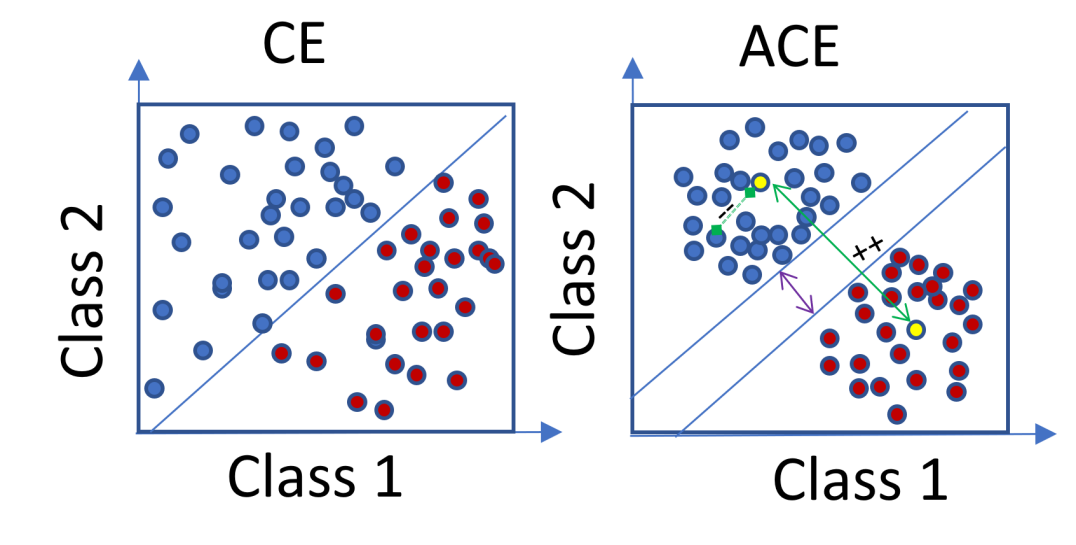
Figure 1: A visual representation of the decision boundary between two classes using Cross Entropy loss (left) and Adversarial Cross Entropy (right). Two terms of the loss are shown as follows: 1) Marginal learning is to ensure the every-class features are assembled while emptying the decision boundary amongst classes (purple line), and 2) Contrastive to contrast between positive and negative classes (green line)

For a long time, the main objective function for training deep learning algorithms is cross-entropy (CE) with several forms. It is responsible to map the corresponding class among the label such that each class is represented by a probability in the output space. Then, the highest class values are chosen to be the targets. The CE objective function can be formulated as follows:

$$\mathcal{L}_{CE}=-\sum_{i}^{K}\log\frac{e^{W^{T}_{y_{i}}x_{i}}}{\sum_{j}{e^{W^{T}_{j}x_{i}}}},$$ (1)

where, $\textbf{x}_{i}\in\mathcal{R}^{d}$ represents deep features of the $i$-th training sample, $y_{i}$ is the corresponding label. $W$ is the trainable parameters of the last linear layer, which is responsible for prediction.

Although CE is the main loss function for most of the learning algorithms, which fails to map to the correct class in the case of boundary samples. If a sample belongs to the class $1$, but similar to the class $2$ features, CE wrongly maps it to the class $1$, as shown in Figure 1. For instance, noisy data or poisoned data can easily trick CE. Therefore, the whole deep learning algorithms become obsolete behind CE shortcomings. Diving deeply into the origins of this problem, it was concluded that boundaries among the classes should be separated as far as possible to get rid of the overlapping between the classes’ features. To address this issue, the model’s features should be learned in a discrimination policy. This main idea is to force CE to learn contrastive features. This way of learning can be achieved by various methods, such as penalizing the Euclidean difference between features and their centers. This forces a margin in the latent space to widen the gap between the classes or push the classes’ centers as farthest as possible from each other. The center loss proved a high improvement in the discrimination between classes’ features by minimizing the intra-classes variability [31]. The following equation shows the center loss calculation.

$$\mathcal{L}_{dis}(\textbf{f}_{i},y)=\frac{1}{n}\sum_{i}\parallel f_{i}-w_{y_{i}}^{c}\parallel_{2}^{2}$$ (2)

where $(\textbf{f}_{i},y)$ is the set of learned features and $w_{y_{i}}^{c}$ are set of learned weights equivalent to the size of the class.

These weights are considered as classes’ centers used to compute the factor of discrimination. The marginal softmax is used as discrimination means to predict well in the case of very high similarity amongst features, such as face verification and noisy data.

$$\mathcal{L}_{marg}=-\sum_{i}^{K}\log\frac{e^{W^{T}_{y_{i}}x_{i}-m}}{e^{W^{T}_{y_{i}}x_{i}-m}+\sum_{j\neq y_{i}}{e^{W^{T}_{y_{j}}x_{i}}}}$$ (3)

where $m$ is the margin to force between the classes’ features each other. The second constraint is to keep the distance among positive classes and negative ones as far as possible, which can be achieved by increasing the distance between the classes’ centers. Marginal softmax forces the features to assemble around their centers, however, it does not ensure various features to be as far as possible. For this purpose, we need another force to balance the distribution of the features to keep the features assembled around their centers and as farthest as possible from each other.

Suppose $w^{c}\in\mathcal{R}^{n\times d}$, where $d$ is the size of the features while $n$ is the total number of classes. Specifically, if $w_{y_{i}}^{c}$ denotes the set of weights of the corresponding class and $w_{j}^{c}$ refers to weights of other classes, the distance between $w_{y_{i}}^{c}$ and $w_{j}^{c}$ should be managed according to the following equation.

$$\mathcal{L}_{contr}=\frac{1}{k}\sum_{i}\frac{\ \ \ \ \ \ \parallel x_{i}-w^{c}_{y_{i}}\ \parallel_{2}}{1+\sum\limits_{\begin{subarray}{c}j\neq i\end{subarray}}\parallel x_{i}-w^{c}_{j}\parallel_{2}},$$ (4)

where the numerator enforces the feature to gather around their centers and the dividend forces the negative classes’ features to be away as far as possible.

The total objective function considers two main constraints: discriminative using Eq. 3, and contrastive using Eq. 4. The supervision process will be jointly trained to ensure both discriminability conditions that are satisfied. The following equation shows the joint loss:

$$\mathcal{L}=\mathcal{L}_{marg}+\mathcal{L}_{contr}$$ (5)

$$\mathcal{L}=-\sum\limits_{\begin{subarray}{c}i\end{subarray}}\log\frac{e^{W^{T}_{y_{i}}x_{i}-m}}{e^{W^{T}_{y_{i}}x_{i}-m}+\sum\limits_{\begin{subarray}{c}j\neq y_{i}\end{subarray}}{e^{W^{T}_{y_{j}}x_{i}}}}+\frac{1}{k}\sum\limits_{\begin{subarray}{c}i\end{subarray}}\frac{\ \ \ \ \ \ \parallel x_{i}-w^{c}_{j}\ \parallel_{2}}{\sum\limits_{\begin{subarray}{c}j\neq i\end{subarray}}\parallel w_{y_{i}}^{c}-w^{c}_{j}\parallel_{2}},$$ (6)

IV Experiments and Result Explanation

In this section, the implementation details of the proposed method are summarised. Afterward, qualitative details are listed in table formats to show the results in comparison to the most recent methods. Generally, the proposed method outperforms several state-of-the-art techniques and introduces a new defense model against adversarial attacks on selected datasets [22, 32]. All the experiments were conducted on Pytorch 1.5 with Quadro 6000 24-GPU memory under Ubuntu 18.

IV-A Implementation Details

Char-CNN is used as the core of the proposed method as the objective function that is embedded in the architecture. We conducted our experiments on different attacks, including [7], FGSM [8] and PGD [19]. The parameters of the core architecture are the default ones of Char-CNN [32], the number of training epochs is $100$, the learning rate is $0.001$, while the batch size is selected to be $128$.

IV-B Results and Discussion

IV-B1 Continuous Attacks

Firstly, attacks, involving FGSM and PGD, are used to hack the model. The attacks generate various text according to the budget scale ($\epsilon$), however, it changes the text to be closer to noise than adversarial attacks. Though continuous attacks belong to the area of noise, it improves the total performance against various types of attacks. From this perspective, we compare our method to the continuous attacks to show our method effectiveness. The proposed method is compared with three baselines as follows: 1) Cross-Entropy (CE) loss, 2) Center loss [31], and 3) marginal CE [4]. The comparison was conducted in two cases: testing-time attacking (i.e. ’no defense’), and adversarial training settings, which attack in the training and the testing time. For parameters, $10$ is the number of iterations for poisoning the sample, whereas the perturbation budget is $8/255$ and $16/255$, respectively.

TABLE I: Comparison between the proposed method and the baseline approaches for UNSW_NB15 dataset.

$\epsilon=8/255$
	No Defense				Adversarial Training
Defenses	Char-CNN	Center [31]	Marginal CE [4]	ours	Char-CNN	Center [31]	Marginal CE [4]	ours
FGSM	49	31	51	58.5	57	44	57.5	65.5
PGD	40	24	41.5	52	47.2	34	35	58.
$\epsilon=16/255$
FGSM	41	29	38	52.9	40.5	36	53.8	61.2
PGD	33	27.3	31	48	41	31.4	27	38

For continuous attacks, we selected one dataset (UNSW_NB15 [22]) to demonstrate a comparison between our proposed methods and other compelling ones. Table I shows the comparison between our method and other methods. Table I (FGSM row) for budget scale $8/255$ shows that the proposed method beats the three baseline approaches by more than $6\%$ in case of ’no defense’. Further, baselines achieved $49\%$, $31\%$, $51\%$ for CE, Center loss, Marginal CE, respectively, whereas our method was able to achieve $58.5\%$. In the case of perturbation scale $=16/255$, our method was able to outperform all the baselines by a reasonable margin of $\approx 12\%$. PGD is known as a strong attack because it works iteratively to generate an adversarial sample rather than one step (FGSM). Table I (PGD row), for budget scale $8/255$, shows that the proposed method beats the three baseline approaches by more than $10\%$ in case of ’no defense’.

Further, the baselines achieved $40\%$, $24\%$, $41.5\%$ for CE, Center loss, Marginal CE, respectively, whereas our method was able to achieve $52\%$. Notably, Marginal CE behaves better than the other two methods with a PGD attack. In the case of perturbation scale $=16/255$, our method was able to outperform all the baselines by a large margin of $15\%$ with PGD attack. Similarly, our method outperforms the state-of-the-art in the adversarial settings in the two various perturbation scales. Likewise, our method outperforms the baselines in adversarial training, while it achieved $65\%$ and $61.2\%$ against FGSM for the two perturbation scales.

IV-B2 Discrete Attacks

In typical adversarial attacks, gradients are the main contributor to guide the modifications to generate an adversarial sample. However, it is not feasible in discrete data (text-data samples) because the domain is so vast as well as it does not perceive the reader (it is a sort of noise). To this end, we use heuristic methods to generate an adversarial sample from the important tokens of the input. Then, we use swap, insertion, deletion, or move methods to craft the input and generate imperceivable text that can evade the algorithm.

Due to the lack of consensus about the methods of attacks and the less number of defenses, results are shown with one baseline comparison (CE). Regarding databases, we use 7 publicly-used datasets [32] along with the Spam dataset [20] to prove the significance of our defense. This set of datasets covers various NLP-tasks such as sentiment analysis, text classification, and spam detection. Char-CNN [32] is used as a backbone with default parameters unless it is stated. The perturbation budget is selected to be $30$.

Regarding generating adversarial examples, we follow [6] to attack the datasets in black-box settings. We generate 4 types of scoring combinations as follows: Replace-1 Scoring (R1S), Temporal Head Scoring (THS), Temporal Tail Scoring (TTS), and Combined (THS + TTS). This step is followed by heuristic methods to change the input sample $x_{i}$. These methods can be listed as follows: (1) Swap: Uses swapped characters to generate an adversarial sample. (2) Substitution: Uses substituted characters to generate an adversarial sample. (3) Deletion: Through the character’s deletion, an adversarial sample is generated. (4) Insertion: Through the character’s insertion, an adversarial sample is generated.
Random & Gradient scoring In this setting, a word is chosen randomly to be changed with one of the above heuristic functions. It does not have any specific method to follow. In gradient-based scoring, the gradient is used to determine the important tokens in the context. It uses the size of the gradient to decide about the important words. In Figure 2, our proposed method behavior is shown against eight-large datasets. Overall, the DBPedia dataset is the easiest to defend whereas securing Amazon Full Review dataset is the most difficult.

TABLE II: Comparison between baseline CE and our method over 8-large datasets. This highlights the accuracy in the case of random scoring.

	Original	Random		Gradient
		CE [7]	Ours	CE [7]	Ours
AG’s News	90.0	89.3	85.6	62.3	82.9
Amazon Review Full	62.0	61.1	68.3	47.0	62.5
Amazon Review Polarity	95.2	93.9	88.7	84.3	93.2
DBPedia	98.4	95.2	86.1	92.9	95.9
Yahoo! Answers	71.0	65.7	67.1	43.5	51.0
Yelp Review Full	63.5	60.9	60.8	45.7	53.4
Yelp Review Polarity	95.3	95.4	88.6	84.8	91.3
Enron Spam Email	95.6	67.8	82.9	69.0	78.4

Table II summarizes the comparison between the baseline and our method. It is clear that our method outperforms the gradient method on all the datasets with margins vary from 3.0 to 20.6 for DBPedia and AG’s News, respectively. In contrast, CE baseline in random settings outperforms our method on AG’s News, Amazon Review Polarity, DBPedia, Yelp Review Full, and Yelp Review Polarity dataset whereas we can beat in Amazon Review Full, Yahoo! Answers, Spam Email. Since random scoring does not follow any algorithmic way, the results are unpredictable and will be changing over the repetition.

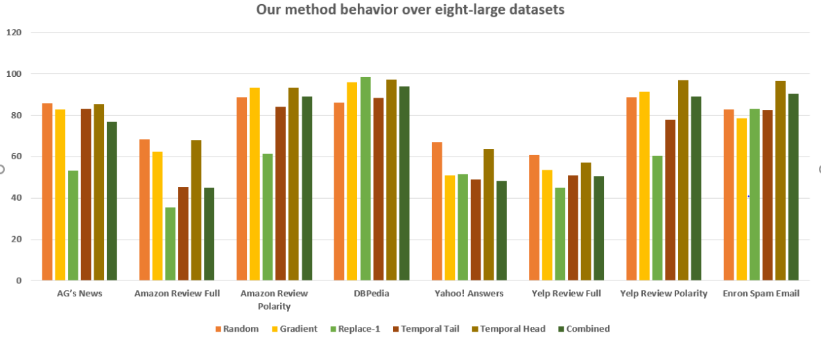
Figure 2: A visual representation for the behavior of our method against six attacks on eight-public-large datasets [32].

Replace-1 Scoring (R1S) will be according to the following equation:

$$R1S(x_{i})=F(x_{1},x_{2},...,x_{i},...,x_{n})-F(x_{1},x_{2},...,\tilde{x_{i}},...,x_{n})$$ (7)

where $\tilde{x_{i}}$ is chosen to be out of the vocabulary to limit the search space.

TABLE III: Comparison between baseline CE and our method over 8-large datasets. This highlights the accuracies in the case of Replace-1 settings.

	Original	Replace-1
		CE [7]	Ours	Improvement
AG’s News	90.0	30.8	53.2	22.4
Amazon Review Full	61.1	25.6	35.5	9.9
Amazon Review Polarity	95.2	46.4	61.5	15.1
DBPedia	98.4	74.9	98.5	23.6
Yahoo! Answers	71.0	30.0	51.5	21.5
Yelp Review Full	63.5	27.6	45.0	12.4
Yelp Review Polarity	95.3	42.8	60.5	17.7
Enron Spam Email	95.6	76.4	83.0	6.6

Table III shows the results of our defense and comparison with state-of-the-art. Both methods use $\epsilon=30$ as a distance to edit the input samples to generate adversarial samples. The results reveal that our method outperforms the baseline in Replace-1 attack by a significant margin that varies from $6.6$ to $23.6$. CE was able to get $30.8$, $25.6$, $46.4$, $74.9$, $30.0$, $27.6$, $42.8$, and $76.4$, whereas our method reported $53.2$, $35.5$, $61.5$, $98.5$, $51.5$, $45.0$, $60.5$ and $83.0$ for AG’s News, Amazon Review Full, Amazon Review Polarity, DBPedia, Yahoo! Answers, Yelp Review Full, Yelp Review Polarity, and Enron Spam Email, respectively.

Temporal-Head Scores (THS) This type of scoring uses sequential predictions of the character $x_{i}$ up to $i^{th}$ subtracted from the model’s prediction of $x_{i}$ up to $i-1$ as follows:

$$THS(x_{i})=F(x_{1},x_{2},...,x_{i-1},x_{i})-F(x_{1},x_{2},...,x_{i-1})$$ (8)

TABLE IV: Comparison between baseline CE and our method over 8-large datasets. This highlights the accuracies in the case of Temporal-head settings.

	Original	Temporal Head
		CE [7]	Ours	Improvement
AG’s News	90.0	74.1	85.5	1.4
Amazon Review Full	61.1	58.1	68.0	9.9
Amazon Review Polarity	95.2	91.6	93.2	1.6
DBPedia	98.4	95.7	97.2	1.5
Yahoo! Answers	71.0	56.8	63.8	7.0
Yelp Review Full	63.5	51.3	57.0	5.7
Yelp Review Polarity	95.3	86.5	97.0	10.5
Enron Spam Email	95.6	85.1	96.5	11.4

Table IV shows the results of our defense and comparison with the state-of-the-art. Both methods use $\epsilon=30$ as a distance to edit the input samples to generate adversarial examples. The results reveal that our method outperforms the baseline in the temporal-head settings by a significant margin that varies from $1.4$ to $11.4$. CE was able to get $74.1$, $58.1$, $91.6$, $95.7$, $56.8$, $51.3$, $86.5$ and $85.1$, whereas our method reported $85.5$, $68.0$, $93.2$, $97.2$, $63.8$, $57.0$, $97.0$, and $96.5$ for AG’s News, Amazon Review Full, Amazon Review Polarity, DBPedia, Yahoo! Answers, Yelp Review Full, Yelp Review Polarity, and Enron Spam Email, respectively. Figure 3 demonstrates the comparison of our method’s effectiveness and CE.

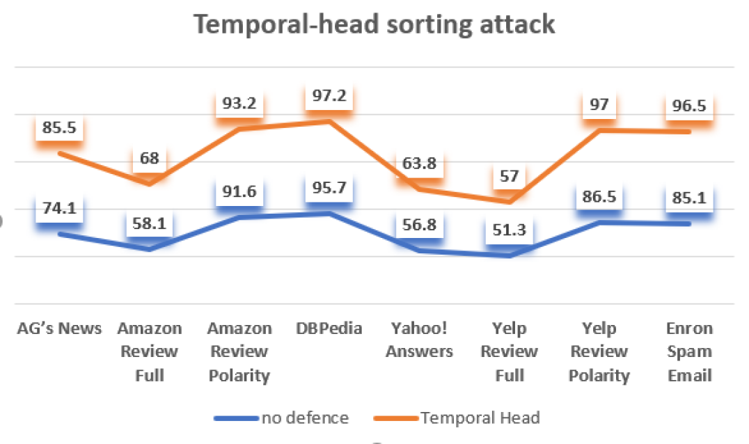
Figure 3: Visualization of our method on the temporal-sorting-based attack over 8 datasets.

Temporal-Tail Scores (TTS) Temporal-tail scores are the complement of THS while it compares the tails of the sentences as follows:

$$TTS(x_{i})=F(x_{i},x_{i+1},...,x_{n})-F(x_{i+1},...,x_{n})$$ (9)

TABLE V: Comparison between baseline CE and our method over 8-large datasets. This highlights the accuracies in the case of Temporal-tail settings.

	Original	Temporal Tail
		CE [7]	Ours	Improvement
AG’s News	90.0	58.6	83.2	24.6
Amazon Review Full	61.1	32.5	45.3	12.8
Amazon Review Polarity	95.2	70.9	84.1	13.2
DBPedia	98.4	88.2	88.3	0.1
Yahoo! Answers	71.0	35.3	49.0	13.7
Yelp Review Full	63.5	35.3	51.0	14.7
Yelp Review Polarity	95.3	71.9	77.9	6.0
Enron Spam Email	95.6	78.7	82.4	3.7

Table V shows the results of our defense and compares it with the state-of-the-art. Both methods use $\epsilon=30$ as a distance to edit the input samples to generate adversarial samples. The results reveal that our method outperforms the baseline in the temporal-head attack by a significant margin varies up to $24.6$ as in AG’s News. CE was able to get $58.6$, $32.5$, $70.9$, $88.2$, $35.3$, $35.3$, $71.9$, and $78.7$, whereas our method reported $83.2$, $45.3$, $84.1$, $88.3$, $49.0$, $51.0$, $77.9$ and $82.4$ for AG’s News, Amazon Review Full, Amazon Review Polarity, DBPedia, Yahoo! Answers, Yelp Review Full, Yelp Review Polarity, and Enron Spam Email, respectively.
Combined Scores Combined scores mainly merging THS and TTS to benefit from both directions of importance. It can be calculated via the following equation.

$$CS(x_{i})=THS(x_{i})+\lambda\ TTS(x_{i})$$ (10)

TABLE VI: Comparison between baseline CE and our method over 8-large datasets in the case of Combined settings.

	Original	Combined
		CE [7]	Ours	Improvement
AG’s News	90.0	60.4	77.0	16.6
Amazon Review Full	61.1	35.0	45.0	10.0
Amazon Review Polarity	95.2	73.5	89.2	15.7
DBPedia	98.4	88.8	93.9	5.2
Yahoo! Answers	71.0	36.6	48.3	11.5
Yelp Review Full	63.5	38.2	50.5	12.3
Yelp Review Polarity	95.3	71.1	89.0	18.9
Enron Spam Email	95.6	75.4	90.2	14.8

Table VI shows the results of our defense and comparison with state-of-the-art. Both methods use $\epsilon=30$ as a distance to edit the input samples to generate adversarial samples. The results reveal that our method outperforms the baseline in the temporal-head attack by a significant margin that varies from $5.2$ to $16.6$. CE was able to get $60.4$, $35.0$, $73.5$, $88.8$, $36.6$, $38.2$, $71.1$, and $75.4$, whereas our method reported $77.0$, $45.0$, $89.2$, $93.9$, $48.3$, $50.5$, $89.0$, and $90.2$ for AG’s News, Amazon Review Full, Amazon Review Polarity, DBPedia, Yahoo! Answers, Yelp Review Full, Yelp Review Polarity, and Enron Spam Email, respectively.

Figure 4 shows the significance of our method on all the datasets. It compares CE to our method. It is clear that our method outperforms in all the attacks except on random one.

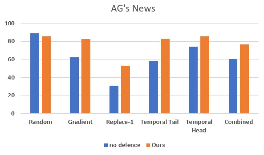
Figure 4: A Comparison between our method and CE on AG’s News datasets for various types of attacks.

V Conclusions

A new marginal-contrastive method has been proposed to defend against adversarial attacks. It is a robust method that can constitute a regularizer to defend against adversarial attacks. The experiments demonstrate that our method can address the issues of adversarial attacks on 1D models. Besides, the experimental comparisons showed that our method achieved very significant outcomes on nine-large-scale datasets under the influence of various attack settings. The impact of adversarial attacks was nearly eliminated in most of the datasets. Eventually, the proposed method highlights the need for further investigations regarding cyber-security schemes on the adversarial paradigm. In the future, marginal-contrastive learning will be extended on various architectures such as 1D, 2D and 3D models.

References

- [1] Evan Ackerman. How drive. ai is mastering autonomous driving with deep learning. IEEE Spectrum Magazine, 1, 2017.
- [2] Moustafa Alzantot, Yash Sharma, Ahmed Elgohary, Bo-Jhang Ho, Mani Srivastava, and Kai-Wei Chang. Generating natural language adversarial examples. arXiv preprint arXiv:1804.07998, 2018.
- [3] Nilaksh Das, Madhuri Shanbhogue, Shang-Tse Chen, Fred Hohman, Li Chen, Michael E Kounavis, and Duen Horng Chau. Keeping the bad guys out: Protecting and vaccinating deep learning with jpeg compression. arXiv preprint arXiv:1705.02900, 2017.
- [4] Jiankang Deng, Jia Guo, Niannan Xue, and Stefanos Zafeiriou. Arcface: Additive angular margin loss for deep face recognition. In Proceedings of the IEEE Conference on Computer Vision and Pattern Recognition, pages 4690–4699, 2019.
- [5] Yinpeng Dong, Fangzhou Liao, Tianyu Pang, Hang Su, Jun Zhu, Xiaolin Hu, and Jianguo Li. Boosting adversarial attacks with momentum. In Proceedings of the IEEE conference on computer vision and pattern recognition, pages 9185–9193, 2018.
- [6] J Gao, B Wang, Z Lin, W Xu, and Y DeepCloak Qi. Masking deep neural network models for robustness against adversarial samples. arxiv 2017. arXiv preprint arXiv:1702.06763.
- [7] Ji Gao, Jack Lanchantin, Mary Lou Soffa, and Yanjun Qi. Black-box generation of adversarial text sequences to evade deep learning classifiers. In 2018 IEEE Security and Privacy Workshops (SPW), pages 50–56. IEEE, 2018.
- [8] Ian J Goodfellow, Jonathon Shlens, and Christian Szegedy. Explaining and harnessing adversarial examples. arXiv preprint arXiv:1412.6572, 2014.
- [9] Han Xu Yao Ma Hao-Chen, Liu Debayan Deb, Hui Liu Ji-Liang Tang Anil, and K Jain. Adversarial attacks and defenses in images, graphs and text: A review. International Journal of Automation and Computing, 17(2):151–178, 2020.
- [10] Thoufique Haq, Jinjian Zhai, and Vinay K Pidathala. Advanced persistent threat (apt) detection center, April 18 2017. US Patent 9,628,507.
- [11] M. Hassanin, S. Khan, and M. Tahtali. A new localization objective for accurate fine-grained affordance segmentation under high-scale variations. IEEE Access, 8:28123–28132, 2020.
- [12] Mohammed Hassanin, Salman Khan, and Murat Tahtali. Visual affordance and function understanding: A survey. arXiv preprint arXiv:1807.06775, 2018.
- [13] Di Jin, Zhijing Jin, Joey Tianyi Zhou, and Peter Szolovits. Is bert really robust? a strong baseline for natural language attack on text classification and entailment. arXiv, pages arXiv–1907, 2019.
- [14] Erik Jones, Robin Jia, Aditi Raghunathan, and Percy Liang. Robust encodings: A framework for combating adversarial typos. arXiv preprint arXiv:2005.01229, 2020.
- [15] Alexey Kurakin, Ian Goodfellow, and Samy Bengio. Adversarial examples in the physical world. arXiv preprint arXiv:1607.02533, 2016.
- [16] Jinfeng Li, Shouling Ji, Tianyu Du, Bo Li, and Ting Wang. Textbugger: Generating adversarial text against real-world applications. arXiv preprint arXiv:1812.05271, 2018.
- [17] Bin Liang, Hongcheng Li, Miaoqiang Su, Pan Bian, Xirong Li, and Wenchang Shi. Deep text classification can be fooled. arXiv preprint arXiv:1704.08006, 2017.
- [18] Xingjun Ma, Bo Li, Yisen Wang, Sarah M Erfani, Sudanthi Wijewickrema, Grant Schoenebeck, Dawn Song, Michael E Houle, and James Bailey. Characterizing adversarial subspaces using local intrinsic dimensionality. arXiv preprint arXiv:1801.02613, 2018.
- [19] Aleksander Madry, Aleksandar Makelov, Ludwig Schmidt, Dimitris Tsipras, and Adrian Vladu. Towards deep learning models resistant to adversarial attacks. arXiv preprint arXiv:1706.06083, 2017.
- [20] Vangelis Metsis, Ion Androutsopoulos, and Georgios Paliouras. Spam filtering with naive bayes-which naive bayes? In CEAS, volume 17, pages 28–69. Mountain View, CA, 2006.
- [21] Nour Moustafa, Kim-Kwang Raymond Choo, Ibrahim Radwan, and Seyit Camtepe. Outlier dirichlet mixture mechanism: Adversarial statistical learning for anomaly detection in the fog. IEEE Transactions on Information Forensics and Security, 14(8):1975–1987, 2019.
- [22] Nour Moustafa and Jill Slay. Unsw-nb15: a comprehensive data set for network intrusion detection systems (unsw-nb15 network data set). In 2015 military communications and information systems conference (MilCIS), pages 1–6. IEEE, 2015.
- [23] Aamir Mustafa, Salman Khan, Munawar Hayat, Roland Goecke, Jianging Shen, and Ling Shao. Adversarial defense by restricting the hidden space of deep neural networks. arXiv preprint arXiv:1904.00887, 2019.
- [24] Taesik Na, Jong Hwan Ko, and Saibal Mukhopadhyay. Cascade adversarial machine learning regularized with a unified embedding. arXiv preprint arXiv:1708.02582, 2017.
- [25] Nicolas Papernot, Patrick McDaniel, Ian Goodfellow, Somesh Jha, Z Berkay Celik, and Ananthram Swami. Practical black-box attacks against machine learning. In Proceedings of the 2017 ACM on Asia conference on computer and communications security, pages 506–519. ACM, 2017.
- [26] Nicolas Papernot, Patrick McDaniel, Somesh Jha, Matt Fredrikson, Z Berkay Celik, and Ananthram Swami. The limitations of deep learning in adversarial settings. In 2016 IEEE European Symposium on Security and Privacy (EuroS&P), pages 372–387. IEEE, 2016.
- [27] Nicolas Papernot, Patrick McDaniel, Xi Wu, Somesh Jha, and Ananthram Swami. Distillation as a defense to adversarial perturbations against deep neural networks. In 2016 IEEE Symposium on Security and Privacy (SP), pages 582–597. IEEE, 2016.
- [28] Marco Tulio Ribeiro, Sameer Singh, and Carlos Guestrin. Semantically equivalent adversarial rules for debugging nlp models. In Proceedings of the 56th Annual Meeting of the Association for Computational Linguistics (Volume 1: Long Papers), pages 856–865, 2018.
- [29] Jacob Steinhardt, Pang Wei W Koh, and Percy S Liang. Certified defenses for data poisoning attacks. In Advances in neural information processing systems, pages 3517–3529, 2017.
- [30] Christian Szegedy, Wojciech Zaremba, Ilya Sutskever, Joan Bruna, Dumitru Erhan, Ian Goodfellow, and Rob Fergus. Intriguing properties of neural networks. arXiv preprint arXiv:1312.6199, 2013.
- [31] Yandong Wen, Kaipeng Zhang, Zhifeng Li, and Yu Qiao. A discriminative feature learning approach for deep face recognition. In European conference on computer vision, pages 499–515. Springer, 2016.
- [32] Xiang Zhang, Junbo Zhao, and Yann LeCun. Character-level convolutional networks for text classification. In Advances in neural information processing systems, pages 649–657, 2015.
- [33] Zhengli Zhao, Dheeru Dua, and Sameer Singh. Generating natural adversarial examples. arXiv preprint arXiv:1710.11342, 2017.