Convergence Rates for Multi-classs Logistic Regression Near Minimum

Abstract

In the current paper we provide constructive estimation of the convergence rate for training a known class of neural networks: the multi-class logistic regression. Despite several decades of successful use, our rigorous results appear new, reflective of the gap between practice and theory of machine learning. Training a neural network is typically done via variations of the gradient descent method. If a minimum of the loss function exists and gradient descent is used as the training method, we provide an expression that relates learning rate to the rate of convergence to the minimum. The method involves an estimate of the condition number of the Hessian of the loss function. We also discuss the existence of a minimum, as it is not automatic that a minimum exists. One method of ensuring convergence is by assigning positive probabiity to every class in the training dataset.

Introduction

Multi-class logistic regression is a common machine learning tool that is a generalization of logistic regression, the generalization being that more than 2 classes are allowed [3], [5]. There have been few documented studies on the mathematics of multi-class logistic regression, and to the authors’ knowledge, none discuss in depth the properties of this simple neural network. [5] derives the Hessian for multi-class logistic regression, but the spectrum was not investigated. [6] has given a linear algebra-centric derivation of the Hessian for a feedforward and simple recurrent neural network whose loss function minimizes a sum of squares, expressing the Hessian as a sum of Kronecker products. There was also brief mention of the bounds of eigenvalues in terms of the summands, but these bounds were not investigated in detail. [4] derived the Hessian for various components of a feedforward network, an approach that was referred to as Hessian backpropagation.[2] derives the Hessian for a (similar) feedforward network with a sum of squares loss function but does not discuss spectral properties.

In this article we investigate spectral properties of the Hessian for multi-class logistic regression and as a consequence we provide the convergence rate near the minimum should it exist. More generally, we discuss the optimization landscape of the loss function including existence of the minimum.

Througout the paper we will consider matrices of various sizes. The vector space of all $p$ by $q$ ($p\times q$) matrices will be denoted by $L(\mathbbm{R}^{q},\mathbbm{R}^{p})$ and every such matrix $A$ is identified with a linear operator $A:\mathbbm{R}^{p}\to\mathbbm{R}^{q}$.

Assume we have a matrix $\mathbf{X}\in L(\mathbbm{R}^{N},\mathbbm{R}^{D})$ whose columns represent a sample, and a target matrix $\mathbf{T}\in L(\mathbbm{R}^{D},\mathbbm{R}^{C})$ where an entry $t_{i}^{(n)}$ ($i^{th}$ row and $n^{th}$ column of $\mathbf{T}$ ) is the probability that the $n^{th}$ sample ($n^{th}$ column of $\mathbf{X}$) belongs to class $i$. We require $\sum_{i=1}^{C}t^{(n)}_{i}=1,\ t^{(n)}_{i}\geq 0$. In the simplest example of multi-class logistic regression, each column of $\mathbf{X}$ belongs to one class so that $t_{i}^{(n)}\in\{0,1\}$ for $\ 1\leq i\leq C$ where $C$ is the number of classes. Define $y^{(n)}_{i}=\sigma^{(i)}\left(\mathbf{W}\mathbf{x}^{(n)}\right)$, where $\boldsymbol{\sigma}:\mathbbm{R}^{C}\to\mathbbm{R}^{C}$ is given by the formula

$$\sigma^{(i)}(\mathbf{u})=\frac{e^{u_{i}}}{\sum_{j=1}^{C}e^{u_{j}}}.$$ (1)

and where $\mathbf{W}\in L(\mathbbm{R}^{D},\mathbbm{R}^{C})$. The function $\boldsymbol{\sigma}$ is known as “softmax”. Consider the function $L:L(\mathbbm{R}^{D},\mathbbm{R}^{C})\to\mathbbm{R}$ given by

$$L(\mathbf{W};\mathbf{X},\mathbf{T})=-\sum_{n=1}^{N}\sum_{i=1}^{C}t_{i}^{(n)}\log y_{i}^{(n)}.$$ (2)

In this equation $\mathbf{W}$ plays a role of a variable, and $\mathbf{X}$, $\mathbf{T}$ are merely parameters. When it is clear from the context what $\mathbf{X}$ and $\mathbf{T}$ is, we will simply write $L(\mathbf{W})$ instead of $L(\mathbf{W};\mathbf{X},\mathbf{T})$, or $L(\mathbf{W};\mathbf{X})$ when it is clear what $\mathbf{T}$ is. On occasions, however, we will need to consider $L$ with different values of $\mathbf{X}$ or $\mathbf{T}$ in the same context, and then we will use the notation $L(\mathbf{W};\mathbf{X})$ or even $L(\mathbf{W};\mathbf{X},\mathbf{T})$. The quantity $L(\mathbf{W};\mathbf{X},\mathbf{T})$ defined by equation (2) is commonly known as the cross-entropy, and it can also be interpreted as negative log-likelihood. The problem of training is the problem of finding the optimal weight matrix $\widehat{\mathbf{W}}$ which minimizes $L(\mathbf{W})$:

$$\widehat{\mathbf{W}}=\operatorname{argmin}_{\mathbf{W}\in L(\mathbbm{R}^{D},\mathbbm{R}^{C})}L(\mathbf{W}).$$ (3)

In other words, (3) is equivalent to finding $\mathbf{W}$ such that the probability of observing the samples is maximized, where $y_{i}^{(n)}$ is the computed probability that the $n^{th}$ sample belongs to class $i$.

In [7], the formulas for the Fréchet derivative, gradient, and second Fréchet derivative of $L(\mathbf{W})$ are given respectively as:

$$DL(\mathbf{W})\mathbf{V}=\sum_{n=1}^{N}-(\mathbf{t}^{(n)}-\mathbf{y}^{(n)})^{\intercal}\,\mathbf{V}\,\mathbf{x}^{(n)},$$ (4)

$$\nabla L(\mathbf{W})=-\sum_{n=1}^{N}\left(\mathbf{t}^{(n)}-\mathbf{y}^{(n)}\right)\left(\mathbf{x}^{(n)}\right)^{\intercal}=-(\mathbf{T}-\mathbf{Y})\,\mathbf{X}^{\intercal},$$ (5)

$$D^{2}L(\mathbf{W})(\mathbf{U},\mathbf{V})=\sum_{n=1}^{N}{\mathbf{x}^{(n)}}^{\intercal}\,\mathbf{U}^{\intercal}\mathbf{Q}^{(n)}\mathbf{V}\,\mathbf{x}^{(n)}.$$ (6)

where $\mathbf{Q}^{(n)}=\mathrm{diag}(\mathbf{y}^{(n)})-\mathbf{y}^{(n)}\,{\mathbf{y}^{(n)}}^{\intercal}$. In [7] a number of fundamental properties of $L$ and its derivatives were shown. We summarize them below, along with additional background-type facts.

1. The quadratic form induced by the bilinear form $D^{2}L(\mathbf{W})$ given by (6) is non-negative definite for all $\mathbf{W}$.

2. If $\mathbf{X}$ has rank $D$ with $D\leq N$ (the condition $D\leq N$ means the number of samples is large compared to the dimension of each sample) then the quadratic form induced by $D^{2}L(\mathbf{W})$ is positive definite on the subspace $Z\subseteq L(\mathbbm{R}^{D},\mathbbm{R}^{C})$ with column means equal to 0. This subspace can also be defined arithmetically by

   $$Z=\{\mathbf{W}\in L(\mathbbm{R}^{D},\mathbbm{R}^{C})\,:\,\mathbbm{1}^{\intercal}\mathbf{W}=0\}$$

   where $\mathbbm{1}\in\mathbbm{R}^{C}$ is the vector of 1’s. More precisely, there is a constant $b>0$ such that for every $\mathbf{W}\in L(\mathbbm{R}^{D},\mathbbm{R}^{C})$ and $\mathbf{V}\in Z$

   $$D^{2}L(\mathbf{W})(\mathbf{V},\mathbf{V})\geq b\|\mathbf{V}\|^{2}.$$

   The choice of the norm is immaterial, but some calculations are facilitated by using the Frobenius norm.

3. The loss function $L$ posseses a shift invariance property. More precisely, let us consider an orthogonal decomposition

   $$L(\mathbbm{R}^{D},\mathbbm{R}^{C})=Z\oplus\Gamma$$

   where $\Gamma=Z^{\perp}$ is the orthogonal complement. This vector subspace can be given more explicitly as

   $$\Gamma=\{\mathbbm{1}\cdot\mathbf{c}^{\intercal}\,:\,\mathbf{c}\in\mathbbm{R}^{C}\}.$$

   These are exactly the matrices which have identical entries in each column. The shift invariance is expressed as follows: for every $\mathbf{W}\in L(\mathbbm{R}^{D},\mathbbm{R}^{C})$ and every $\mathbf{c}\in\mathbbm{R}^{D}$

   $$L\left(\mathbf{W}+\mathbbm{1}\cdot\mathbf{c}^{\intercal}\right)=L(\mathbf{W}).$$

   Therefore it is sufficient to study $L$ restricted to $Z$, which will be denoted by $L|Z$.

4. The fact that $D^{2}L(\mathbf{W})$ induces a positive definite quadratic form on $Z$ implies that $L|Z$ is a locally strongly convex function (cf. the Appendix A). It is not true that a locally strongly convex function must have a global minimum (an explicit example is given in [7]). However, a necessary and sufficient condition for $L|Z$ (and thus $L$) to have a global minimum is that there exists a critical point of $L$: a $\mathbf{W}$ such that $\nabla L(\mathbf{W})=0$. Furthermore, if a critical point exists then

   $$\lim_{\mathbf{V}\to\infty,\mathbf{V}\in Z}L(\mathbf{V})=\infty$$

   It should be noted that this condition is necessary and sufficient for a convex function $L$ to have a unique global minimum on a subspace $Z$.

In the current paper we address two important issues:

1. The existence of a global minimum of the loss function $L$ (Section 2).

2. Effective bounds on the convergence of algorithms which find the minimum of $L$. For instance, one may then use the gradient descent formula to minimize $L$:

   $$\mathbf{W}_{n}=\mathbf{W}_{n-1}-\eta\,\boldsymbol{\nabla}L(\mathbf{W}_{n-1}).$$ (7)

   The speed of convergence is given in terms of the condition number of the Hessian matrix of $L$ at the minimum. Equivalently we may seek constants $b,B\in\mathbbm{R}$, $0<b\leq M<\infty$, such that for every $\mathbf{V}\in Z$ we have:

   $$b\,\|\mathbf{V}\|^{2}\leq D^{2}L(\mathbf{W})(\mathbf{V},\mathbf{V})\leq B\,\|\mathbf{V}\|^{2}.$$

   It will be seen that such bounds exist and can be constructively found (Section 3).

Existence of the Minimum

The immediate objective is to prove that the loss function $L$ has a critical point under suitable assumptions. For the sake of clarity, we adopt some definitions and notations:

Definition 1 (Positivity of a Matrix).

A positive matrix is a real matrix $\mathbf{A}=[a_{ij}]$ which is positive elementwise: $a_{ij}>0$ for all $i$ and $j$. We write $\mathbf{A}>0$ iff $A$ is a positive matrix.

Definition 2 (Nullspace and Range of a Linear Operator).

For a linear operator $\mathbf{F}$, let $\operatorname{\mathcal{N}}(\mathbf{F})$ and $\operatorname{\mathcal{R}}(\mathbf{F})$ denote the nullspace (kernel) and range (image) of $\mathbf{F}$, respectively.

Clearly, a sufficient condition for $\nabla L(\mathbf{W})=0$ is that $\mathbf{T}=\mathbf{Y}$ where $\mathbf{Y}=\boldsymbol{\sigma}(\mathbf{W}\mathbf{X})$ (activations of the neural network). Also, $\mathbf{T}>0$ follows from $\mathbf{T}=\mathbf{Y}$. However, It is possible to have a minimum $\mathbf{W}$ for which $\mathbf{T}\neq\mathbf{Y}$. It is also possible to have a global minimum for $\mathbf{T}\not>0$. However, as $\nabla L(\mathbf{W})=-(\mathbf{T}-\mathbf{Y})\,\mathbf{X}^{\intercal}=0$, the necessary and sufficient condition for $\mathbf{W}$ to be a critical point is:

$$\operatorname{\mathcal{N}}(\mathbf{T}-\mathbf{Y})\supseteq\operatorname{\mathcal{R}}\left(\mathbf{X}^{\intercal}\right)=\operatorname{\mathcal{N}}(\mathbf{X})^{\perp}.$$ (8)

The following lemma fully resolves the issue of the existence and calculating the minimum in the easiest, but still useful, case:

Lemma 1.

Assume $\mathbf{T}>0$, $N=D$, and that $\mathbf{X}$ is invertible. Then a minimum of $L$ exists and every minimum $\widetilde{\mathbf{W}}$ is given by

$$\widetilde{\mathbf{W}}=\mathbf{R}\mathbf{X}^{-1}+\mathbbm{1}\mathbf{c}^{\intercal}$$

where where $\mathbf{R}=\ln(\mathbf{T})$ (elementwise logarithm) and $\mathbf{c}\in\mathbbm{R}^{D}$ is arbitrary. Exactly one of the minima belongs to $Z$ and is

$$\widetilde{\mathbf{W}}=\left(\mathbf{I}-\frac{1}{C}\mathbbm{1}\mathbbm{1}^{\intercal}\right)\mathbf{R}\mathbf{X}^{-1}$$

and is also the matrix obtained from $\mathbf{R}\mathbf{X}^{-1}$ obtained by subtracting from each column its mean.

Proof.

Suppose that $\nabla L(\mathbf{W})=0$. As in this case the operator $\mathbf{X}^{\intercal}$ is invertible as well, and therefore surjective: $\operatorname{\mathcal{R}}\left(\mathbf{X}^{\intercal}\right)=\mathbbm{R}^{N}$ (the entire codomain). Hence, by Lemma 8, $\operatorname{\mathcal{N}}(\mathbf{T}-\boldsymbol{\sigma}(\mathbf{W}\mathbf{X}))=\mathbbm{R}^{N}$, which implies $\mathbf{T}-\boldsymbol{\sigma}(\mathbf{W}\mathbf{X})=0$. Thus, $\mathbf{T}=\boldsymbol{\sigma}(\mathbf{W}\mathbf{X})$. Also, $\mathbf{T}=\boldsymbol{\sigma}(\mathbf{R})$ and therefore $\boldsymbol{\sigma}(\mathbf{R})=\boldsymbol{\sigma}(\mathbf{W}\mathbf{X})$ . Lemma 6 yields:

$$\mathbf{R}=\mathbf{W}\mathbf{X}+\mathbbm{1}\cdot\mathbf{c}^{\intercal}$$ (9)

for some $\mathbf{c}\in\mathbbm{R}^{D}$. Therefore,

$$\mathbf{W}=\mathbf{R}\mathbf{X}^{-1}-\mathbbm{1}\cdot\mathbf{c}^{\intercal}\mathbf{X}^{-1}=\mathbf{R}\mathbf{X}^{-1}-\mathbbm{1}\cdot\mathbf{d}^{\intercal}$$ (10)

where $\mathbf{d}=(\mathbf{X}^{-1})^{\intercal}\mathbf{c}$ is also arbitrary. Clearly, the only way to put $\mathbf{W}$ in $Z$ is to pick $\mathbf{d}$ to be the vector of column means of $\mathbf{R}\mathbf{X}^{-1}$. Formally, assuming $\mathbf{W}\in Z$ and multiplying (10) by $\mathbbm{1}^{\intercal}$ on the left we obtain:

$$0=\mathbbm{1}^{\intercal}\mathbf{W}=\mathbbm{1}^{\intercal}\mathbf{R}\mathbf{X}^{-1}-\mathbbm{1}^{\intercal}\mathbbm{1}\mathbf{d}^{\intercal}=\mathbbm{1}^{\intercal}\mathbf{R}\mathbf{X}^{-1}-C\mathbf{d}^{\intercal}.$$

(Note: $C$ is the number of classes.) Hence

$$\mathbf{d}^{\intercal}=\frac{1}{C}\mathbbm{1}^{\intercal}\mathbf{R}\mathbf{X}^{-1}$$

i.e. the row vector of column means of $\mathbf{R}\mathbf{X}^{-1}$. Plugging into equation (10) we obtain

$$\mathbf{W}=\mathbf{R}\mathbf{X}^{-1}-\frac{1}{C}\mathbbm{1}\mathbbm{1}^{\intercal}\mathbf{R}\mathbf{X}^{-1}=\left(\mathbf{I}-\frac{1}{C}\mathbbm{1}\mathbbm{1}^{\intercal}\right)\mathbf{R}\mathbf{X}^{-1}$$

as claimed. The operator $\mathbf{I}-(1/C)\mathbbm{1}\mathbbm{1}^{\intercal}$ is recognized as the orthogonal projection on the space of vectors of mean $0$. ∎

Corollary 1.

If $\mathbf{T}>0$ and $\operatorname{\mathrm{rank}}\kern-1.0pt\left(\mathbf{X}\right)=D$, then a global minimum of $L=L(\cdot;\mathbf{X},\mathbf{T})$ exists. Furthermore, the global minimum exists and is unique within subspace $Z$.

Proof.

Consider an invertible submatrix $\widetilde{\mathbf{X}}\in L(\mathbbm{R}^{D},\mathbbm{R}^{D})$ of $\mathbf{X}$ along with the corresponding loss function $\widetilde{L}=L(\cdot;\widetilde{\mathbf{X}})$. Let $\widetilde{\widetilde{\mathbf{X}}}$ be the complementary matrix of $\widetilde{\mathbf{X}}$ within $\mathbf{X}$ and let $\widetilde{\widetilde{L}}=L(\cdot;\widetilde{\widetilde{\mathbf{X}}})$. Then $L=\widetilde{L}+\widetilde{\widetilde{L}}$. We can use Lemma 1 to deduce that $\tilde{L}$ has a unique global minimum on $Z$ and is also locally strongly convex on $Z$. By Lemma 8

$$\lim_{\mathbf{W}\to\infty,\mathbf{W}\in Z}\widetilde{L}(\mathbf{W})=\infty.$$

The loss function $\widetilde{\widetilde{L}}$ is bounded below by 0 and also convex (but perhaps not locally strongly convex). Therefore,

$$\lim_{\mathbf{W}\to\infty,\mathbf{W}\in Z}L(\mathbf{W})=\infty.$$

Applying Lemma 8 again we deduce that $L(\mathbf{W})$ has a unique global minimum within $Z$. Therefore $L$ has global minima differing by a matrix of the form $\mathbbm{1}\cdot\mathbf{c}$. ∎

It is clear that when $\mathbf{X}$ is not square, that (9) may not have a solution, even if $\mathbf{T}>0$. This can be seen more clearly by taking transposes and rearranging the equation $\mathbf{C}=\mathbf{W}\mathbf{X}-\mathbf{R}$, where $\mathbf{C}=\mathbbm{1}\cdot\mathbf{c}^{\intercal}\in\Gamma$:

$$\mathbf{C}^{T}=\mathbf{X}^{T}\mathbf{W}^{T}-\mathbf{R}^{T}.$$ (11)

Noting that the columns of $\mathbf{C}^{T}$ are the same, this implies

$$\mathbf{X}^{T}(\mathbf{w}^{(i)}-\mathbf{w}^{(j)})=\mathbf{r}^{(i)}-\mathbf{r}^{(j)}$$ (12)

where $\mathbf{w}^{(i)}$ is a column of $\mathbf{W}^{T}$ and $\mathbf{r}^{(i)}$ a column of $\mathbf{R}^{T}$. If $\operatorname{\mathrm{rank}}\kern-1.0pt\left(\mathbf{X}\right)=D<N$, then clearly there exist $\mathbf{T}$ (and hence $\mathbf{R}$) such that (12) does not hold for a given $\mathbf{X}$, since $\mathbf{X}^{T}$ does not span $\mathbbm{R}^{N}$ for $N>D$. This does not mean that $\nabla L(\mathbf{W})=0$ does not have a solution since we did not rule out the possibility of this equation being satisfied without $\mathbf{T}=\mathbf{Y}$. However, the following theorem takes care of this and broadens the previous statements on the existence of the minimum:

Theorem 2.1 (Existence of minimum, $\operatorname{\mathrm{rank}}\kern-1.0pt\left(\mathbf{X}\right)=D$).

Let us assume that $\mathbf{T}>0$ and that $\operatorname{\mathrm{rank}}\kern-1.0pt\left(\mathbf{X}\right)=D$. Then a minimum of $L=L(\cdot;\mathbf{X},\mathbf{C})$ exists. Furthermore a unique minimum exists within a subspace $Z$. All minima of $L$ may be obtained by additionally translating by a matrix of the form $\mathbbm{1}\cdot\mathbf{c}^{\intercal}$, $\mathbf{c}\in\mathbbm{R}^{D}$.

Proof.

The idea is to study the behavior of $L(\beta\mathbf{W})$ as $\beta\;\to\;\infty$. According to Lemma 9, if $\mathbf{u}^{(n)}=\mathbf{W}\mathbf{x}^{(n)}$, we have:

$$\lim_{\beta\to\infty}L(\beta\mathbf{W}) =-\sum_{n=1}^{N}\sum_{i=1}^{C}t_{i}^{(n)}\lim_{\beta\to\infty}\log\sigma^{(i)}\left(\mathbf{u}^{(n)}\right)$$

$$=\sum_{n=1}^{N}\sum_{i=1}^{C}t_{i}^{(n)}\lim_{\beta\to\infty}\left(-\log\sigma^{(i)}\left(\mathbf{u}^{(n)}\right)\right).$$

As all terms in the sum are non-negative, the limit is infinite iff there is an $i$ and $n$ such that

1. $t_{i}^{(n)}>0$, which is automatically guaranteed if $\mathbf{T}>0$, and

2. $$\lim_{\beta\to\infty}\left(-\log\sigma^{(i)}\left(\mathbf{u}^{(n)}\right)\right)=\infty,\quad\text{or, equivalently,}\quad\lim_{\beta\to\infty}\sigma^{(i)}\left(\mathbf{u}^{(n)}\right)=0,$$

Acording to Lemma 9, the second condition is satisfied when $i\notin J_{n}$, where $J_{n}$ is the set of indices $i$ for which $u_{i}^{(n)}$ is maximal. Thus, there must be a row $\mathbf{W}_{i}$ of $\mathbf{W}$ such that $\mathbf{W}_{i}\mathbf{x}^{(n)}$ is not maximal. Only when all vectors $\mathbf{W}\mathbf{x}^{(n)}$ are multiples of $\mathbbm{1}$ this is not possible. Thus, any matrix $\mathbf{W}$ such that $L(\beta\mathbf{W})$ is bounded as $\beta\to\infty$ satisfies

$$\mathbf{W}\mathbf{X}=\mathbbm{1}\mathbf{c}^{\intercal}$$

for some $\mathbf{c}\in\mathbbm{R}^{N}$. If we additionally assume that $\mathbf{W}\in Z$, we will show that $\mathbf{W}\mathbf{X}=0$. The argument consists in pre-multiplying by $\mathbbm{1}^{\intercal}$:

$$0=\mathbbm{1}^{\intercal}\mathbf{W}\mathbf{X}=\mathbbm{1}^{\intercal}\mathbbm{1}\mathbf{c}^{\intercal}=C\mathbf{c}^{\intercal}.$$

(Note: $C$ is the number of classes.) Hence $\mathbf{c}=0$ and $\mathbf{W}\mathbf{X}=0$ as claimed.

The condition $\mathbf{W}\mathbf{X}=0$ may be rephrased as $\operatorname{\mathcal{N}}(\mathbf{W})\supseteq\operatorname{\mathcal{R}}(\mathbf{X})$. As $\dim\operatorname{\mathcal{R}}(\mathbf{X})=\operatorname{\mathrm{rank}}\kern-1.0pt\left(\mathbf{X}\right)=D$, we have $\operatorname{\mathcal{R}}(\mathbf{X})=\mathbbm{R}^{D}$, i.e. $\mathbf{X}$ is a surjective as a linear operator. There $\operatorname{\mathcal{N}}(\mathbf{W})=\mathbbm{R}^{D}$, i.e. $\mathbf{W}=0$. We thus have shown that for every $\mathbf{W}\in Z\setminus\{0\}$, $\lim_{\beta\to\infty}L(\beta\mathbf{W})=\infty$. By Lemma 8 there is a unique global minimum of $L|Z$. ∎

When $\operatorname{\mathrm{rank}}\kern-1.0pt\left(\mathbf{X}\right)$ is arbitrary, a similar result holds, but it requires the use of some abstract linear algebra, both in its formulation as well as in the proof. Thus, we separated it from the more simple-minded Theorem 2.1.

Occasionally we use the notion of orthogonality in the space of matrices $L(\mathbbm{R}^{p},\mathbbm{R}^{q})$. This requires us to define a scalar product. The only product used in the current paper is the Frobenius inner product:

$$\langle\mathbf{U},\mathbf{V}\rangle=\operatorname{Tr}{\mathbf{U}^{T}\mathbf{V}}=\sum_{i=1}^{q}\sum_{j=1}^{p}u_{ij}v_{ij}.$$

Theorem 2.2 (Existence of minimum, $\operatorname{\mathrm{rank}}\kern-1.0pt\left(\mathbf{X}\right)$ arbitrary).

Let us assume that $\mathbf{T}>0$ and $\mathbf{X}\in L(\mathbbm{R}^{N},\mathbbm{R}^{D})$ be an arbitrary matrix. Then a global minimum of $L=L(\cdot;\mathbf{X},\mathbf{T})$ exists.

Furthermore,

1. let $\mathbf{F}_{\mathbf{X}}\,:\,L(\mathbbm{R}^{D},\mathbbm{R}^{C})\to L(\mathbbm{R}^{N},\mathbbm{R}^{C})$ be a linear operator given by $\mathbf{F}_{\mathbf{X}}(\mathbf{W})=\mathbf{W}\mathbf{X}$;

2. let $Z_{0}\subseteq Z$ be a subspace of $Z$ defined by $Z_{0}=\operatorname{\mathcal{N}}\left(\mathbf{F}_{\mathbf{X}}\right)\cap Z$;

3. let $Z_{1}\subseteq Z$ be the complement of $Z_{0}$, so that $Z=Z_{0}\oplus Z_{1}$ (direct sum).

Then

1. $L|Z$ is invariant under shift by a vector in $Z_{0}$;

2. $L|Z_{1}$ has a unique global minimum;

3. all global minima of $L|Z$ can be obtained by translating the minimum of $L|Z_{1}$ by vectors in $Z_{0}$;

4. all minima of $L$ may be obtained by adding a matrix of the form $\mathbbm{1}\cdot\mathbf{c}^{\intercal}$, $\mathbf{c}\in\mathbbm{R}^{D}$ to a minimum of $L|Z$.

Proof.

The proof remains identical to the proof of Theorem 2.1, until the final stage, when we can no longer claim that $\mathbf{W}\mathbf{X}=0$ implies $\mathbf{W}=0$. Thus, we modify the proof from this point on.

Let $\Gamma_{1}=\{\mathbbm{1}\cdot\mathbf{c}^{\intercal}\,:\,\mathbf{c}\in\mathbbm{R}^{N}\}$ be a subspace of $L(\mathbbm{R}^{N},\mathbbm{R}^{C})$. We have defined a similar space $\Gamma\subseteq L(\mathbbm{R}^{D},\mathbbm{R}^{C})$ which differs only by the dimensions of the matrices, which is the orthogonal complement of $Z$. It is easy to see that $\mathbf{F}_{\mathbf{X}}(\Gamma)\subseteq\Gamma_{1}$ because $\mathbf{F}_{\mathbf{X}}(\mathbbm{1}\mathbf{c}^{\intercal})=\mathbbm{1}\mathbf{c}^{\intercal}\mathbf{X}=\mathbbm{1}(\mathbf{X}^{\intercal}\mathbf{c})^{\intercal}\in\Gamma_{1}$. Let $\Gamma_{2}=\mathbf{F}_{\mathbf{X}}^{-1}(\Gamma_{1})$ ($\Gamma_{2}\supseteq\Gamma$) be a vector subspace of $L(\mathbbm{R}^{D},\mathbbm{R}^{C})$. We claim that $\Gamma_{2}\cap Z\subseteq\operatorname{\mathcal{N}}(\mathbf{F}_{\mathbf{X}})$. Indeed, we have shown that $\mathbf{F}_{\mathbf{X}}(\mathbf{W})=\mathbbm{1}\cdot\mathbf{c}^{\intercal}$ and $\mathbf{W}\in Z$ implies that $\mathbf{W}\in\operatorname{\mathcal{N}}\left(\mathbf{F}_{\mathbf{X}}\right)$. The consequence is that $L|Z$ can be factored through the natural projection onto the quotient space $Z/(\Gamma_{1}\cap Z)$, which is the “right” domain of $L$. In fact, it is the same trick that resulted in introduction of $Z$: $L$ factored through the natural projection onto $L(\mathbbm{R}^{D},\mathbbm{R}^{C})/\Gamma$ (another way to understand shift invariance with respect to shifts by elements of $\Gamma$). But also $L|Z$ is invariant under shifts by elements of $\Gamma_{1}\cap Z$. Indeed, since $\mathbf{Y}=\left(\boldsymbol{\sigma}\circ\mathbf{F}_{\mathbf{X}}\right)(\mathbf{W})$ then $L$ depends on $\mathbf{W}$ only through $\mathbf{Y}$. Since $\mathbf{F}_{\mathbf{X}}$ is a linear operator, $\mathbf{Y}$, and therefore $L$, are invariant under shifts by vectors in $\operatorname{\mathcal{N}}(\mathbf{F}_{\mathbf{X}})$. And $L|Z$ is invariant under shits by vectors in $\operatorname{\mathcal{N}}(\mathbf{F}_{\mathbf{X}})\cap Z$.

It can be seen that $Z_{0}=\operatorname{\mathcal{N}}(\mathbf{F}_{\mathbf{X}})\cap Z$ represents “wasted parameters” of the model, as there is no reduction of $L$ by descending along the directions belonging to this subspace (in fact, $L$ is constant along those directions). Eliminating these parameters leads to considering $L$ on the subspace $Z_{1}\subseteq Z$. The function $L|Z_{1}$ does not contain any directions from $\Gamma_{1}$ and thus

$$\lim_{\mathbf{W}\to\infty,\mathbf{W}\in Z_{1}}L(\mathbf{W})=\infty.$$

Applying Lemma 8 we deduce that $L$ has a global minimum in $Z_{1}$. This minimum could be non-unique because a priori we do not know that $L|Z_{1}$ is locally strongly convex without assuming that $\operatorname{\mathrm{rank}}\kern-1.0pt\left(\mathbf{X}\right)=D$. However locally strong convexity still holds, and this could be shown by repeating the proof in [7], which would show that $D^{2}L(\mathbf{W})$ induces a positive definite quadratic form on $Z_{1}$. We will briefly outline this argument. Due to the explicit formula for $D^{2}L(\mathbf{W})$ (equation (6)) we have

$$D^{2}L(\mathbf{W})(\mathbf{U},\mathbf{U})=\sum_{n=1}^{N}\left(\mathbf{U}\,\mathbf{x}^{(n)}\right)^{\intercal}\mathbf{Q}^{(n)}\left(\mathbf{U}\,\mathbf{x}^{(n)}\right).$$

In [7] it was shown that $\mathbf{Q}^{(n)}$ is a non-negative definite matrix, with a simple eigenvalue $0$ with eigenvector $\mathbbm{1}$. Hence, $D^{2}L(\mathbf{W})(\mathbf{U},\mathbf{U})>0$ unless

$$\mathbf{U}\,\mathbf{x}^{(n)}=c_{n}\mathbbm{1},\quad n=1,2,\ldots,N.$$

Equivalently, $\mathbf{U}\mathbf{X}=\mathbbm{1}\mathbf{c}^{\intercal}\in\Gamma_{1}$, i.e., $\mathbf{U}\in\mathbf{F}_{X}^{-1}(\Gamma_{1})$. If we additionally assume that $\mathbf{U}\in Z$ then $\mathbf{U}\in\mathbf{F}_{X}^{-1}(\Gamma_{1})\cap Z\subseteq\operatorname{\mathcal{N}}(\mathbf{F}_{X})\cap Z=Z_{0}$. As $Z_{1}$ is a complement of $Z_{0}$ in $Z$, $D^{2}L(\mathbf{W})(\mathbf{U},\mathbf{U})\neq 0$ (equivalently, $>0$) for all $\mathbf{U}\in Z_{1}$. This demonstrates that $L|Z_{1}$ is a locally strongly convex function, and yields the conclusion of the proof. ∎

There is also an alternative proof, which we will present here, using a coordinate-dependent style of argument. Conceptually, this proof reduces the proof of Theorem 2.2 to applying Theorem 2.1. This proof has an additional value, as it has a practical approach to finding the minimum of $L$ and reducing the number of weights (parameters of the neural model under consideration).

Proof.

(An alternative proof of Theorem 2.2) Let $K=\operatorname{\mathrm{rank}}\kern-1.0pt\left(\mathbf{X}\right)$. Let us identify $\mathbbm{R}^{D}$ with $\mathbbm{R}^{K}\oplus\mathbbm{R}^{D-K}$ where $\mathbbm{R}^{K}$ is embedded into $\mathbbm{R}^{D}$ as the first $K$ coordinates and $\mathbbm{R}^{D-K}$ as the last $D-K$ coordinates. There is an invertible matrix $\mathbf{S}\in L(\mathbbm{R}^{D},\mathbbm{R}^{D})$ such that $\operatorname{\mathcal{R}}(\mathbf{S}\mathbf{X})=\mathbbm{R}^{K}\subseteq\mathbbm{R}^{D}$. Then we have the following obvious change of variables formula:

$$L(\mathbf{W};\mathbf{X})=L(\widetilde{\mathbf{W}};\widetilde{\mathbf{X}}).$$

where $\widetilde{\mathbf{W}}=\mathbf{W}\mathbf{S}^{-1}$ and $\widetilde{\mathbf{X}}=\mathbf{S}\mathbf{X}$. Therefore the minima of $L(\cdot;\mathbf{X})$ and $L(\cdot;\widetilde{\mathbf{X}})$ are the same up to a linear change of variables in the space of weight matrices. In particular, the global minima correspond and strong convexity is preserved. Furthermore, we consider the following partitions of $\widetilde{\mathbf{X}}$ and $\widetilde{\mathbf{W}}$ into submatrices,

$$\widetilde{\mathbf{X}}=\left[\begin{array}[]{c}\widetilde{\kern 0.0pt\raisebox{0.0pt}[0.85pt]{$\widetilde{\mathbf{X}}$}}\\ \hline\cr\mathbf{0}\end{array}\right]\quad\text{and}\quad\widetilde{\mathbf{W}}=\left[\begin{array}[]{c|c}\widetilde{\kern 0.0pt\raisebox{0.0pt}[0.85pt]{$\widetilde{\mathbf{W}}$}}&\mathbf{*}\end{array}\right],$$

where $\widetilde{\kern 0.0pt\raisebox{0.0pt}[0.85pt]{$\widetilde{\mathbf{X}}$}}$ is a submatrix of $\widetilde{\mathbf{X}}$ consisting of the first $K$ rows of $\widetilde{\mathbf{X}}$ (a $K\times N$ matrix of rank $K$), $\mathbf{0}$ is a $(D-K)\times N$ matrix of zeros, and where $\widetilde{\kern 0.0pt\raisebox{0.0pt}[0.85pt]{$\widetilde{\mathbf{W}}$}}$ is submatrix of $\widetilde{\mathbf{W}}$ consisting of the first $K$ columns of $\widetilde{\mathbf{W}}$, while $\mathbf{*}$ is a “wildcard” submatrix consisting of the last $D-K$ columns of $\widetilde{\mathbf{W}}$. The expression $L\left(\widetilde{\mathbf{W}};\widetilde{\mathbf{X}}\right)$ does not explictly depend on the last $D-K$ columns of the matrix $\widetilde{\mathbf{W}}$ and therefore

$$L(\widetilde{\mathbf{W}};\widetilde{\mathbf{X}})=L(\widetilde{\kern 0.0pt\raisebox{0.0pt}[0.85pt]{$\widetilde{\mathbf{W}}$}};\widetilde{\kern 0.0pt\raisebox{0.0pt}[0.85pt]{$\widetilde{\mathbf{X}}$}}).$$

Also, $L(\mathbf{W};\mathbf{X})=L(\widetilde{\kern 0.0pt\raisebox{0.0pt}[0.85pt]{$\widetilde{\mathbf{W}}$}};\widetilde{\kern 0.0pt\raisebox{0.0pt}[0.85pt]{$\widetilde{\mathbf{X}}$}})$ and there is correspondence between the global minima of $L(\cdot;\mathbf{X})$ and $L(\cdot;\widetilde{\kern 0.0pt\raisebox{0.0pt}[0.85pt]{$\widetilde{\mathbf{X}}$}})$, but it is not a 1:1 correspondence because many matrices $\mathbf{W}$ correspond to a single matrix $\widetilde{\kern 0.0pt\raisebox{0.0pt}[0.85pt]{$\widetilde{\mathbf{W}}$}}$ by varying the last $D-K$ columns of $\widetilde{\mathbf{W}}=\mathbf{W}\mathbf{S}^{-1}$.

By Theorem 2.1, $L(\cdot;\widetilde{\kern 0.0pt\raisebox{0.0pt}[0.85pt]{$\widetilde{\mathbf{X}}$}})$ is locally strongly convex on $Z\subseteq L(\mathbbm{R}^{K},\mathbbm{R}^{C})$ and has a unique global minimum (say, $\widetilde{\kern 0.0pt\raisebox{0.0pt}[0.85pt]{$\widetilde{\mathbf{W}}$}}$) there. (Note that the domain of $L(\cdot;\widetilde{\kern 0.0pt\raisebox{0.0pt}[0.85pt]{$\widetilde{\mathbf{X}}$}})$ is $L(\mathbbm{R}^{K},\mathbbm{R}^{C})$, so $Z$ denotes a different vector space than in prior discussion.) All global minima of $L(\cdot;\widetilde{\mathbf{X}})$ are obtained by varrying the wildcard portion of $\widetilde{\mathbf{W}}$. Finally, we identify the wildcard portion as $\operatorname{\mathcal{N}}(\mathbf{F}_{\widetilde{\mathbf{X}}})$ and the change of coordinates $\mathbf{W}\mapsto\widetilde{\mathbf{W}}=\mathbf{W}\mathbf{S}^{-1}$ maps bijectively $\mathbf{W}\in\operatorname{\mathcal{N}}(\mathbf{F}_{\mathbf{X}})$ to $\widetilde{\mathbf{W}}\in\operatorname{\mathcal{N}}(\mathbf{F}_{\widetilde{\mathbf{X}}})$. It also maps $Z$ bijectively onto itself. These observations imply all statements of the theorem. ∎

Here we illustrate some scenarios in which a minimum does or does not exist.

Example 1 (No minimum exists).

Let

$$\mathbf{X}=\begin{bmatrix}1&0\\ 0&1\\ \end{bmatrix}\ \ \mathbf{T}=\begin{bmatrix}0&0\\ 1&1\\ \end{bmatrix}.$$

Then

$$\mathbf{\widehat{\mathbf{W}}}=\begin{bmatrix}-1/2&-1/2\\ 1/2&1/2\\ \end{bmatrix}$$

is a direction for which $L(\beta\widehat{\mathbf{W}})$ is bounded, implying that no minimum is reached for this sample.

Example 2 (Minimum exists).

Let

$$\mathbf{X}=\begin{bmatrix}1&0&1\\ 0&1&1\\ \end{bmatrix}\ \ \mathbf{T}=\begin{bmatrix}0&0&1\\ 1&1&0\\ \end{bmatrix}.$$

Then one cannot find $\widehat{\mathbf{W}}$ such that $L(\beta\widehat{\mathbf{W}})$ is bounded, implying that a minimum exists. Explicitly, from the matrices given, one needs $w_{21}\geq w_{11},\ w_{22}\geq w_{12},\ w_{11}+w_{12}\geq w_{21}+w_{22}$. This is only satisfied if $\mathbf{W}$ has identical entries which corresponds to $Z\ni\mathbf{W}=0$.

Example 3 (Minimum exists).

In this example, $L$ is not locally strongly convex because $\mathbf{X}$ does not have rank $D$. Let

$$\mathbf{X}=\begin{bmatrix}1&-1&-1&1\\ 1&-1&-1&1\\ 1&-1&-1&1\\ -1&1&1&-1\\ -3&3&3&-3\\ -3&3&3&-3\\ \end{bmatrix}\ \ \mathbf{T}=\begin{bmatrix}1&1&0&0\\ 0&0&1&1\\ 0&0&0&0\\ 0&0&0&0\\ \end{bmatrix}.$$

A matrix $\mathbf{W}$ that gives a minimum can be found by inspection to be

$$\mathbf{W}=\begin{bmatrix}1&1&-1&1&2&-2\\ 1&1&-1&1&1&-1\\ -1&-1&1&-1&4&-4\\ -1&-1&1&-1&-7&7\\ \end{bmatrix}$$

as can be verified that $\nabla L(\mathbf{W})=0$.

Rate of Convergence of Gradient Descent Near Minimum

We assume that a minimum of the loss function exists. One can define a continuous map based upon (7), as

$$\boldsymbol{\Phi}(\mathbf{W})=\mathbf{W}-\eta\,\boldsymbol{\nabla}L(\mathbf{W}).$$ (13)

Then Taylor expanding $\boldsymbol{\Phi}(\mathbf{W})$ about the global minimum $\mathbf{\widehat{W}}$, we can obtain approximate expressions for $\boldsymbol{\Phi}(\mathbf{W}^{(n+1)})$ and $\boldsymbol{\Phi}(\mathbf{W}^{(n)})$. Subtracting one of the Taylor expansions from the other, we find $\mathbf{W}^{(n+2)}-\mathbf{W}^{(n+1)}\approx D\boldsymbol{\Phi}(\mathbf{\widehat{W}})(\mathbf{W}^{(n+1)}-\mathbf{W}^{(n)})$ or

$$\mathbf{e}^{(n+1)}\approx D\boldsymbol{\Phi}(\mathbf{\widehat{W}})\mathbf{e}^{(n)}$$ (14)

where $\mathbf{e}^{(n+1)}$ is the error for the ${(n+1)}\text{st}$ iteration. We want to bound $\left\lVert D\boldsymbol{\Phi}(\mathbf{\widehat{W}})\right\rVert_{2}=\left\lVert\mathbf{I}-\mathbf{H}(\mathbf{\widehat{W}})\right\rVert_{2}$ and of course ensure that it is less than 1. We require $\left\lVert\mathbf{I}-\mathbf{H}(\mathbf{\widehat{W}})\right\rVert_{2}$ must be within the interval $[-\theta,\theta]$, where $\theta\in(0,1)$. Let $\lambda_{max},\lambda_{min}$ be the largest and smallest eigenvalues of $\mathbf{H}$. As noted in [7],

$$-\theta \leq 1-\eta\,\lambda_{max}$$

$$\theta \geq 1-\eta\,\lambda_{min}.$$

This implies that for a contraction, it is necessary to have

$$K\leq\frac{1+\theta}{1-\theta}$$

where

$$K=\frac{\lambda_{max}}{\lambda_{min}}$$

is also the condition number of the Hessian. Next, we provide bounds on $\lambda_{min},\lambda_{max}$.

Hessian Matrix for Loss Function

Working with the Hessian for the space $Z$ is difficult. Instead, we work with the isomorphic space $L(\mathbbm{R}^{C-1},\mathbbm{R}^{N})$ via a mapping $L(\mathbbm{R}^{C-1},\mathbbm{R}^{N})\to Z$ given by $\mathbf{S}\mapsto\mathbf{KS}$ where $\mathbf{K}$ has dimension $C$ by $C-1$ and $\mathbf{S}$ has dimension $C-1$ by $N$, and where the column means are 0. The mapping is invertible so we have $\mathbf{KS}\ni Z\to\mathbf{S}\in L(\mathbbm{R}^{C-1},\mathbbm{R}^{N})$. A choice for $\mathbf{K}$ is

$$\mathbf{K}=\begin{bmatrix}1&0&0&\dots 0\\ 0&1&0&\dots 0\\ 0&0&1&\dots 0\\ &&\ddots&\\ 0&0&0&1\\ -1&-1&-1&-1\end{bmatrix}.$$ (15)

Another choice is to choose $\mathbf{K}$ so that the mapping $\mathbf{KS}\to\mathbf{S}$ is an isometry, i.e.

$$\mathbf{K}^{T}\mathbf{K}=\mathbf{I}_{C-1}$$ (16)

and the column means are 0. In both cases $\mathbf{K}$ is in $L(\mathbbm{R}^{C-1},\mathbbm{R}^{C})$. It can be easily shown that if the mapping is an isometry then the induced Hessian on the space $L(\mathbbm{R}^{C-1},\mathbbm{R}^{N})$ has the same eigenvalues as the Hessian defined on the space $Z$. Thus we can study the eigenvalues of our problem by working on the space $L(\mathbbm{R}^{C-1},\mathbbm{R}^{N})$ via an isometry. This is the first motivation for studying the space $L(\mathbbm{R}^{C-1},\mathbbm{R}^{N})$. A second motivation is that one may want to do gradient descent using the space $L(\mathbbm{R}^{C-1},\mathbbm{R}^{N})$ instead of $Z$. One would then need to study the eigenvalues of the induced Hessian on $L(\mathbbm{R}^{C-1},\mathbbm{R}^{N})$ to obtain convergence properties. The eigenvalues will vary depending on the type of $\mathbf{K}$ used. For the moment, assume $\mathbf{X}$ is in $L(\mathbbm{R}^{N},\mathbbm{R}^{N})$. (the general $D\times N$ case will be dealt with later). For simplicity, we just consider one sample and so drop superscripts $(n)$ from the vectors $\mathbf{x},\mathbf{t},\mathbf{y}$. Then, using the Chain rule for Fréchet derivatives, and noting that $\mathbf{W}$=$\mathbf{K}\mathbf{S}$ for some $\mathbf{S}\in L(\mathbbm{R}^{C-1},\mathbbm{R}^{N})$,

$$DL(\mathbf{S})(\mathbf{P})=DL(\mathbf{W})\circ D\mathbf{W}(\mathbf{S})\mathbf{P}=-(\mathbf{t}-\mathbf{y})^{\intercal}\,\mathbf{KP}\,\mathbf{x}.$$ (17)

where $\mathbf{P}$ has the same dimensions as $\mathbf{S}$. From the definition of gradient, one has

$$DL(\mathbf{S})(\mathbf{P})=\langle\nabla L(\mathbf{S}),\mathbf{P}\rangle$$ (18)

where $\langle\cdot,\cdot\rangle=\operatorname{Tr}(\cdot,\cdot)$. It follows

$$-(\mathbf{t}-\mathbf{y})^{\intercal}\,\mathbf{KP}\,\mathbf{x}=\langle\nabla L(\mathbf{S}),\mathbf{P}\rangle.$$ (19)

Using the fact that $\mathbf{a^{\intercal}}\mathbf{b}=\operatorname{Tr}(\mathbf{a^{\intercal}}\mathbf{b})=\operatorname{Tr}(\mathbf{b}\mathbf{a^{\intercal}})$, the previous equation becomes

$$\operatorname{Tr}(-\mathbf{KP}\,\mathbf{x}(\mathbf{t}-\mathbf{y})^{\intercal}\ )=\operatorname{Tr}(-\mathbf{x}(\mathbf{t}-\mathbf{y})^{\intercal}\ \mathbf{KP})=\langle\nabla L(\mathbf{S}),\mathbf{P}\rangle.$$ (20)

From this it follows that

$$\nabla L(\mathbf{S})=-\mathbf{x}(\mathbf{t}-\mathbf{y})^{\intercal}\ \mathbf{K}.$$ (21)

Let $\mathbf{R}\to\mathbf{K}\mathbf{R}$ where $\mathbf{R}\in L(\mathbbm{R}^{C-1},\mathbbm{R}^{N})$ and $\mathbf{K}$ is the same as before. Then similarly, we can write the second derivative in terms of $\mathbf{S}$, acting in the directions of $\mathbf{P}$ and $\mathbf{R}$ as

$$D^{2}L(\mathbf{S})(\mathbf{P},\mathbf{R})=\mathbf{x}^{\intercal}(\mathbf{K}\mathbf{R})^{\intercal}\mathbf{Q}\mathbf{K}\mathbf{P}\mathbf{x}.$$ (22)

We then use the definition of Hessian to write

$$D^{2}L(\mathbf{S})(\mathbf{P},\mathbf{R})=\langle\mathbf{H}(\mathbf{R}),\mathbf{P}\rangle$$ (23)

from which we may write

$$\langle\mathbf{x}\mathbf{x}^{\intercal}(\mathbf{K}\mathbf{R})^{\intercal}\mathbf{Q}\mathbf{K},\mathbf{P}\rangle=\langle\mathbf{H}(\mathbf{R}),\mathbf{P}\rangle$$ (24)

which gives

$$\mathbf{x}\mathbf{x}^{\intercal}(\mathbf{K}\mathbf{R})^{\intercal}\mathbf{Q}\mathbf{K}=\mathbf{H}(\mathbf{R}).$$ (25)

We can apply the operator $\operatorname{\mathbf{Vec}}$ to both sides of the equation to get

$$\operatorname{\mathbf{Vec}}(\mathbf{H}(\mathbf{R}))=\left((\mathbf{K^{T}QK})\otimes(\mathbf{x}\mathbf{x}^{\intercal})\right)\operatorname{\mathbf{Vec}}(\mathbf{R}^{\intercal})$$ (26)

where $\operatorname{\mathbf{Vec}}$ takes a matrix and outputs its columns stacked [7]. Considering contributions from each $\mathbf{x}^{(n)}$, and re-defining $\mathbf{H}$ as the matrix acting on $\operatorname{\mathbf{Vec}}(\mathbf{R})$ we get

$$\mathbf{H}=\sum_{n=1}^{N}\mathbf{H}^{(n)}$$ (27)

where

$$\mathbf{H}^{(n)}=\mathbf{A}^{(n)}\otimes\mathbf{B}^{(n)}$$ (28)

and $\mathbf{A}^{(n)}=\mathbf{K}^{\intercal}\mathbf{Q}^{(n)}\mathbf{K}$, $\mathbf{B}^{(n)}=\mathbf{x}^{(n)}{\mathbf{x}^{(n)}}^{\intercal}$, and the superscript $(n)$ indicates quantities corresponding the the $n^{th}$ sample. Note that $\mathbf{H}$ is in $L(\mathbbm{R}^{N(C-1)},\mathbbm{R}^{N(C-1)})$.

Eigenvalue Bounds when $N=D$

We provide eigenvalue bounds (below and above) on $\mathbf{H}$ necessary for our investigation into convergence rate.

Lemma 2.

$\mathbbm{R}^{N(C-1)}=\bigoplus_{n=1}^{n=N}\operatorname{\mathcal{R}}(\mathbf{H}^{(n)})$

Proof.

Each $\mathbf{H}^{(n)}$ has rank $C-1$ by the rank property of Kronecker products. We also know that the rank of $\mathbf{H}$ is $N(C-1)$ as it is invertible. This implies $\operatorname{\mathcal{R}}(\mathbf{H}^{(i)})\bigcap\operatorname{\mathcal{R}}(\mathbf{H}^{(j)})=\emptyset$ for $i\neq j$. We thus have that $\mathbbm{R}^{N(C-1)}=\bigoplus_{n=1}^{n=N}\operatorname{\mathcal{R}}(\mathbf{H}^{(n)})$. ∎

Let $\lambda_{i}(\mathbf{G})$ denote the $i^{th}$ largest eigenvalue of $\mathbf{G}$, for some Hermitian matrix $\mathbf{G}$, where eigenvalues are reapeated according to their (algebraic) multiplicity.

Lemma 3 (Weyl [1]).

Let $\mathbf{A}$ and $\mathbf{B}$ (not to be confused with our earlier definitions of $\mathbf{A}^{(n)}$ and $\mathbf{B}^{(n)}$ in (28)) be Hermitian and in $L(\mathbbm{R}^{N},\mathbbm{R}^{N})$ with eigenvalues $(\alpha_{i})_{i=1}^{N}$ and $(\beta_{i})_{i=1}^{N}$ sorted in decreasing order. Then

$$\alpha_{i}+\beta_{N}\leq\lambda_{i}(\mathbf{A}+\mathbf{B})\leq\alpha_{i}+\beta_{i}$$ (29)

Corollary 2 (Weyl Perturbation).

Let $\mathbf{A}$ and $\mathbf{B}$ be any two Hermitian operators in $L(\mathbbm{R}^{N},\mathbbm{R}^{N})$ with eigenvalues of $\mathbf{A}$ given by $(\alpha_{i})_{i=1}^{N}$, in decreasing order. Then

$$\alpha_{i}-\left\lVert\mathbf{B}\right\rVert_{2}\leq\lambda_{i}(\mathbf{A}+\mathbf{B})\leq\alpha_{i}+\left\lVert\mathbf{B}\right\rVert_{2}$$ (30)

Corollary 3.

$$\lambda_{N(C-1)}(\mathbf{H})\leq C\min_{1\leq i\leq N}{\left\lVert\mathbf{x}^{(i)}\right\rVert_{2}}$$ (31)

Proof.

Let $\mathbf{A}=\sum_{n=1}^{N-1}\mathbf{H}^{(n)},\ \mathbf{B}=\mathbf{H}^{(N)}$. Then applying (30), we have that

$$\left|\lambda_{N(C-1)}(\mathbf{H})-\lambda_{N(C-1)}\left(\sum_{n=1}^{N-1}\mathbf{H}^{(n)}\right)\right|\leq\left\lVert\mathbf{H}^{(N)}\right\rVert_{2}.$$

Since $\sum_{n=1}^{N-1}\mathbf{H}^{(n)}$ is not full rank, $\lambda_{N(C-1)}\left(\sum_{n=1}^{N-1}\mathbf{H}^{(n)}\right)=0$. Also,

$$\left\lVert\mathbf{H}^{(N)}\right\rVert_{2}=\left\lVert\lambda_{1}(\mathbf{A}^{(N)})\right\rVert_{2}\left\lVert\lambda_{1}(\mathbf{B}^{(N)})\right\rVert_{2}=\left\lVert\lambda_{1}(\mathbf{A}^{(N)})\right\rVert_{2}\left\lVert\mathbf{x}^{(N)}\right\rVert_{2}^{2}$$

where $\mathbf{A}^{(N)}$ and $\mathbf{B}^{(N)}$ are the same as in (28), and where we used the formula for eigenvalues of Kronecker products. Since the choice of $\mathbf{H}^{(N)}$ is arbitrary, we take $\min_{1\leq i\leq N}{\|\mathbf{x}^{(i)}\|_{2}}$. We provide an upper bound for $\left\lVert\lambda_{1}(\mathbf{A}^{(N)})\right\rVert_{2}$ as follows. The fact that $\mathbf{A}^{(N)}$ is positive definite and $\sum_{i=1}^{N}\lambda_{i}\left(\mathbf{A}^{(N)}\right)=\operatorname{Tr}\mathbf{A}^{(N)}$ gives

$$\lambda_{1}\left(\mathbf{A}^{(N)}\right)\leq\operatorname{Tr}{\mathbf{A}^{(N)}}=\operatorname{Tr}(\mathbf{Q}\mathbf{K}\mathbf{K}^{\intercal})\leq\sqrt{\langle\mathbf{Q},\mathbf{Q}\rangle}\sqrt{\langle\mathbf{K}\mathbf{K}^{\intercal},\mathbf{K}\mathbf{K}^{\intercal}\rangle}\leq\sqrt{C}\sqrt{\operatorname{Tr}(\mathbf{K}^{\intercal}\mathbf{K}\mathbf{K}^{\intercal}\mathbf{K})}<C$$

where we use (16). ∎

Corollary 4.

$$\max\left\{\left(\min_{n,i}y_{i}^{(n)}\right)\left(\max_{i}\left\lVert\mathbf{x}^{(i)}\right\rVert_{2}\right),\left(\max_{n,i}y_{i}^{(n)}\right)\left(\min_{i}\left\lVert\mathbf{x}^{(i)}\right\rVert_{2}\right)\right\}\leq\lambda_{1}\left(\mathbf{H}\right)\leq C{\left\lVert\mathbf{X}\right\rVert_{F}}$$ (32)

Proof.

The inequality on the right follows from the triangle inequality applied to $\sum_{n=1}^{N}\mathbf{H}^{(n)}$. For the inequality on the left, similarly as before, let $\mathbf{A}=\mathbf{H}^{(i)}$ and $\mathbf{B}=\mathbf{H}-\mathbf{H}^{(i)}$ for some $1\leq i\leq N$, then apply (29) using the fact that $\mathbf{A}$ is positive semidefinite and singular to get $\max_{1\leq i\leq N}\lambda_{1}\left(\mathbf{H}^{(i)}\right)\leq\lambda_{1}(\mathbf{H})$. Note

$${\max_{i}\lambda_{1}\left(\mathbf{H}^{\left(i\right)}\right)}=\max_{i}\left(\lambda_{1}\left(\mathbf{A}^{(i)}\right)\ \left\lVert\mathbf{x}^{(i)}\right\rVert_{2}\right)\geq\left(\max_{1\leq i\leq N}\lambda_{1}(\mathbf{A}^{(i)})\right)\left(\min_{1\leq i\leq N}\left\lVert\mathbf{x}^{(i)}\right\rVert_{2}\right).$$

Similarly,

$${\max_{i}\lambda_{1}\left(\mathbf{H}^{\left(i\right)}\right)}\geq\left(\min_{1\leq i\leq N}\lambda_{1}(\mathbf{A}^{(i)})\right)\left(\max_{1\leq i\leq N}\left\lVert\mathbf{x}^{(i)}\right\rVert_{2}\right).$$

To bound $\lambda_{1}(\mathbf{A}^{(i)})$ from below, use

$$\lambda_{1}(\mathbf{A}^{(i)})=\sup_{\mathbf{u}}\frac{(\mathbf{u}\mathbf{K})^{\intercal}\mathbf{Q}^{(i)}\mathbf{Ku}}{\lVert\mathbf{u}\rVert^{2}}=\sup_{\mathbf{u}}\frac{(\mathbf{u}\mathbf{K})^{\intercal}\mathbf{Q}^{(i)}\mathbf{Ku}}{\lVert\mathbf{Ku}\rVert^{2}}=\sup_{\mathbf{K}\mathbf{u}}\frac{(\mathbf{u}\mathbf{K})^{\intercal}\mathbf{Q}^{(i)}\mathbf{Ku}}{\lVert\mathbf{Ku}\rVert^{2}}$$

where we use (15). From [7] we know that $\mathbbm{1}$ is the only eigenvector of $\mathbf{Q}$ with eigenvalue $0$, which implies $\left\langle\mathbf{q}^{(i)},\mathbbm{1}\right\rangle=0$, $i=1,2,\ldots C-1$ where $\mathbf{q}^{(i)}$ is an eigenvector of $\mathbf{Q}$ corresponding to the $i^{th}$ largest eigenvalue of $\mathbf{Q}$. From this it follows that

$$\mathbbm{R}^{C}\setminus\{\mathbbm{1}\}=\operatorname{Span}\left\{\mathbf{q}^{(i)}\right\}_{i=1}^{C-1}=\operatorname{Span}\left\{\mathbf{k}^{(i)}\right\}_{i=1}^{C-1}.$$ (33)

For $\mathbf{K}$ given by 15 and 16. Also, recalling from [7] that $\lambda_{1}(\mathbf{Q}^{(n)})\geq\max_{i}{y_{i}^{(n)}}$, we have

$$\lambda_{1}(\mathbf{A}^{(i)})\geq\max_{i}y_{i}^{(i)}$$ (34)

Combining our results,

$$\lambda_{1}\left(\mathbf{H}^{\left(i\right)}\right)\geq\max\left\{\left(\min_{n,i}y_{i}^{(n)}\right)\left(\max_{i}\left\lVert\mathbf{x}^{(i)}\right\rVert_{2}\right),\left(\max_{n,i}y_{i}^{(n)}\right)\left(\min_{i}\left\lVert\mathbf{x}^{(i)}\right\rVert_{2}\right)\right\}$$

∎

Lemma 4.

We have

$$\lambda_{N(C-1)}\left(\mathbf{H}\right)\geq\left(\min_{n,i}\left\lVert\mathbf{x}^{(n)}\right\rVert_{2}^{2}y_{i}^{(n)}\right).$$ (35)

Proof.

For Hermitian matrices, the minimum of the Rayleigh quotient gives the smallest eigenvalue:

$$\lambda_{N(C-1)}\left(\mathbf{H}\right)=\min_{\left\lVert u\right\rVert_{2}=1}\langle u,\mathbf{H}u\rangle=\min_{\left\lVert u\right\rVert_{2}=1}\sum_{n=1}^{N}\langle u,\mathbf{H}^{(n)}u\rangle.$$ (36)

By Lemma 2, write $\mathbf{u}=\sum_{n=1}^{N}\mathbf{u}^{(n)}$ where $\mathbf{u}^{(n)}\in\operatorname{\mathcal{R}}(\mathbf{H}^{(n)})$. Using these facts we get

$$\min_{\|u\|_{2}=1}\sum_{n=1}^{N}\langle u,\mathbf{H}^{(n)}u\rangle\geq\left(\sum_{n=1}^{N}\min_{u^{(n)}\in\operatorname{\mathcal{R}}(\mathbf{H}^{(n)})\setminus\mathbf{0}}\langle u^{(n)},\mathbf{H}^{(n)}u^{(n)}\rangle\right)\bigg{|}_{\left\lVert u\right\rVert_{2}=1}.$$ (37)

Now use $1=\lVert\mathbf{u}\rVert_{2}\leq\sum_{n=1}^{N}\left\lVert\mathbf{u}^{(n)}\right\rVert_{2}$ along with the fact that $\lambda_{N(C-1)}(\mathbf{H}^{(n)})=0$ for all $n$, to find that the right hand side of (37) is greater or equal to

$$\min_{n}\min_{u\in\operatorname{\mathcal{R}}(\mathbf{H}^{(n)})\setminus\mathbf{0},\;\left\lVert u\right\rVert_{2}=1}\left\langle u,\mathbf{H}^{(n)}u\right\rangle.$$ (38)

Let $\mathbf{H}^{(n)}$ have “reduced” spectral resolution $\sum_{j\in S}\alpha_{j}^{(n)}\mathbf{q}_{j}^{(n)}\left(\mathbf{q}_{j}^{(n)}\right)^{T}$, where $S=\{j:\alpha_{j}^{(n)}\neq 0\}$. Then

$$\min_{\mathbf{u}\in\operatorname{\mathcal{R}}(\mathbf{H}^{(n)}),\ \left\lVert u\right\rVert_{2}=1}\left\langle\mathbf{u},\mathbf{H}^{(n)}\mathbf{u}\right\rangle=\min_{i}\left\{\lambda_{i}\left(\mathbf{H}^{(n)}\right)\,:\,\lambda_{i}\left(\mathbf{H}^{(n)}\right)\neq 0\right\}.$$ (39)

Also, by the eigenvalue property of Kronecker products,

$$\min_{i}\left\{\lambda_{i}\left(\mathbf{H}^{(n)}\right):\lambda_{i}\left(\mathbf{H}^{(n)}\right)\neq 0\right\}=\lambda_{C-1}\left(\mathbf{A}^{(n)}\right)\cdot\lVert\mathbf{x}^{(n)}\rVert_{2}^{2}.$$ (40)

For the case in which $\mathbf{K}$ is given by (16), we have

$$\lambda_{C-1}\left(\mathbf{A}^{(n)}\right)=\inf_{\mathbf{u}}\frac{(\mathbf{u}\mathbf{K})^{\intercal}\mathbf{Q}^{(n)}\mathbf{K}\mathbf{u}}{\left\lVert\mathbf{u}\right\rVert_{2}^{2}}=\inf_{\mathbf{u}}\frac{(\mathbf{u}\mathbf{K})^{\intercal}\mathbf{Q}^{(n)}\mathbf{K}\mathbf{u}}{\left\lVert\mathbf{Ku}\right\rVert_{2}^{2}}=\inf_{\mathbf{K}\mathbf{u}}\frac{\mathbf{(uK)^{\intercal}}\mathbf{Q}^{(n)}\mathbf{Ku}}{\left\lVert\mathbf{Ku}\right\rVert_{2}^{2}}.$$

where we use (33). Thus

$$\lambda_{C-1}\left(\mathbf{A}^{(n)}\right)=\min_{i}y_{i}^{(n)}.$$ (41)

Combining this with (40) we get (35). We get a similar result for the case of non-isometric $\mathbf{K}$:

$$\lambda_{C-1}\left(\mathbf{A}^{(n)}\right)=\inf_{\mathbf{u}}\frac{(\mathbf{u}\mathbf{K})^{\intercal}}{\mathbf{Q}^{(n)}\mathbf{K}\mathbf{u}\left\lVert\mathbf{u}\right\rVert_{2}^{2}}\geq\inf_{\mathbf{u}}\frac{(\mathbf{u}\mathbf{K})^{\intercal}\mathbf{Q}^{(n)}\mathbf{K}\mathbf{u}}{\left\lVert\mathbf{K}\mathbf{u}\right\rVert_{2}^{2}}=\min_{i}y_{i}^{(n)}$$

∎

We showed that isometric and non-isometric $\mathbf{K}$ give the same lower bound $\lambda_{C-1}\left(\mathbf{A}^{(n)}\right)\geq\min_{i}y_{i}^{(n)}$. For $\mathbf{K}$ given by (15) we get an inequality, but we have an equality for isometric $\mathbf{K}$. We thus improved that bound (0) given by [6]. The figures below show how $\lambda_{C-1}\left(\mathbf{A}^{(n)}\right)$ behaves when $\mathbf{K}$ is given by (15) and when $y_{i}^{(n)}$ have the same marginal distribution. For each realization, $\{y_{i}\}$ are chosen from a uniform distribution on $(0,1)$ then divided by $\sum_{i=1}^{C}y_{i}$ so that their sum is 1.

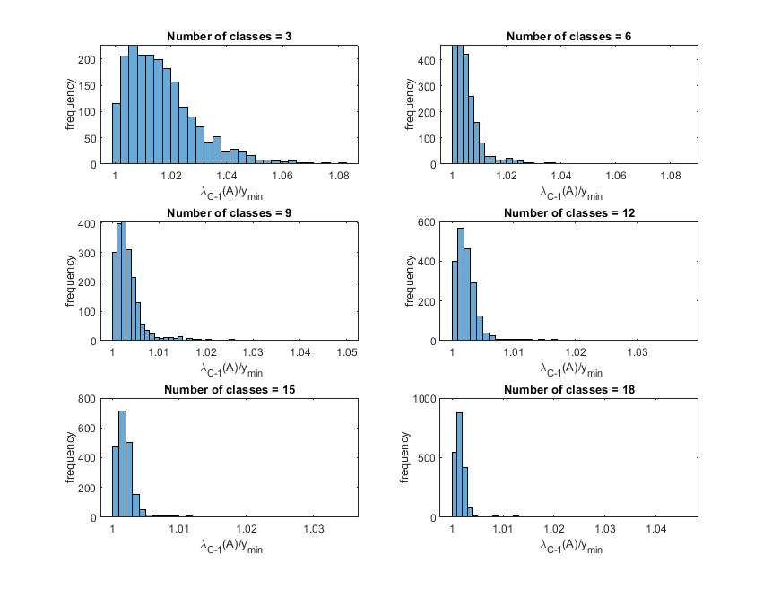
Figure 1: The matrix $\mathbf{K}$ used to compute $\mathbf{A}$ is given by (15). The eigenvalues of $\mathbf{A}$ were computed for $C=3,6,9,12,15,18$. Plots of the frequencies of the ratio $\frac{\lambda_{C-1}\left(A\right)}{y_{min}}$ were made. Each plot corresponds to 2000 realizations.

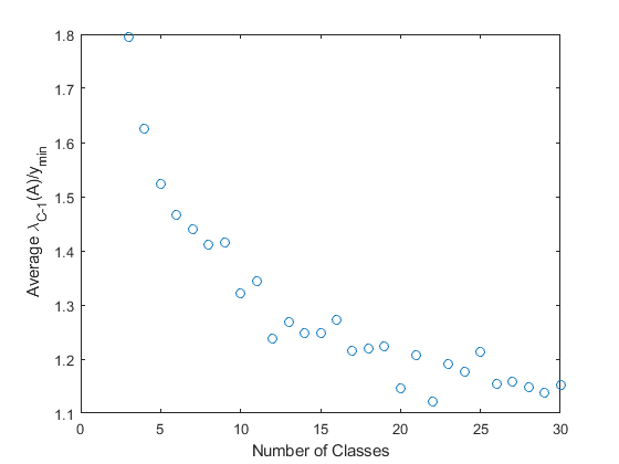
Figure 2: The matrix $\mathbf{K}$ used to compute $\mathbf{A}$ is given by (15). The eigenvalues of $\mathbf{A}$ were computed for $C=3,6,9,12,15,18$. Plots of the frequencies of the ratio $\frac{\lambda_{C-1}\left(A\right)}{y_{min}}$ were made. Each plot corresponds to 2000 realizations.

From the figures, we see that $\lambda_{C-1}\left(\mathbf{A}^{(n)}\right)\to 1$ as $C\to\infty$ if $\{y_{i}\}$ have the same marginal distribution. This begs the question: is this behavior correct, and independent of the way $\{y_{i}\}$ are generated? We start by analyzing the expression

$$\inf_{\mathbf{u}:\lVert\mathbf{u}\rVert_{2}=1}=\frac{(\mathbf{u}\mathbf{K})^{\intercal}\mathbf{Q}^{(n)}\mathbf{K}\mathbf{u}}{\left\lVert\mathbf{u}\right\rVert_{2}^{2}}$$

which we know is bounded below by $\min_{i}y_{i}^{(n)}$. Using the definition of Rayleigh quotient, the figures suggest that there typically exists $\mathbf{u}$ such that $\lVert\mathbf{u}\rVert_{2}=1$ and $\lVert\mathbf{Ku}-\mathbf{q}_{C-1}\rVert_{2}$ is small, and that this approximation gets better as $C\to\infty$, where ${\mathbf{q}}_{C-1}$ is the eigenvector corresponding to the $(C-1)^{st}$ largest eigenvalue of $\mathbf{Q}^{(n)}$. Note $\left\lVert\mathbf{K}\mathbf{u}-\mathbf{q}_{C-1}\right\rVert_{2}$ is small if $\left\lVert\mathbf{u}-\mathbf{\widetilde{q}}_{C-1}\right\rVert_{2}$ is small, where $\mathbf{\widetilde{q}}_{C-1}$ is equal to the first $C-1$ components of $\mathbf{q}_{C-1}$. Now realize that $\mathbf{q}_{C-1}$ (as are all eigenvectors corresponding to non-zero eigenvalue) is in the range of $\mathbf{K}$ since the columns of $\mathbf{K}$ are orthogonal to the the vectors of 1’s. So we may write $\mathbf{q}_{C-1}=\sum_{i=1}^{C-1}\alpha_{i}\mathbf{K}^{(i)}$. Since $\left\lVert\mathbf{q}_{C-1}\right\rVert_{2}=1$, it follows that $\sum_{i=1}^{C-1}\alpha_{i}^{2}+\left(\sum_{i=1}^{C-1}\alpha_{i}\right)^{2}=1$. Let

$$V=\left\{\boldsymbol{\alpha}\in\mathbbm{R}^{C-1}:\sum_{i=1}^{C-1}\alpha_{i}^{2}+\left(\sum_{i=1}^{C-1}\alpha_{i}\right)^{2}=1\right\}.$$

Our discussion can be rephrased as follows: a sufficient condition for which $\lambda_{C-1}\left(\mathbf{A}^{(n)}\right)$ goes to 0 as $C\to\infty$ is: $\min_{x\in S^{C-2}}dist(\boldsymbol{\alpha},\mathbf{x})\to 0$ as $C\to\infty$ given any $\boldsymbol{\alpha}\in V$, where $S^{C-2}$ is the $(C-2)$-dimensional unit sphere. We formalize our discussion in the following lemma:

Lemma 5.

Fix $n$ and assume each $y_{i}^{(n)}$ for $i=1,2,\ldots,C$ has the same marginal distribution. Then $\lambda_{C-1}\left(\mathbf{A}^{(n)}\right)\to\min_{i}y_{i}^{(n)}$ in probability as $C\to\infty$

Proof.

From the preceding discussion, it suffices to show that $\min_{x\in S^{C-2}}\operatorname{dist}(\boldsymbol{\alpha},\mathbf{u})\to 0$ as $C\to\infty$, for any $\boldsymbol{\alpha}\in V$. We do this by showing that $P\left(\left|\sum_{i=1}^{C-1}\alpha_{i}^{2}-1\right|>\epsilon\right)\to 0$ as $C\to\infty$. For the proof, we drop the superscript $(n)$ from $\mathbf{A}^{(n)}$ and $y_{i}^{(n)}$ . Denote $q_{i}$ to be the $i^{th}$ component of $\mathbf{q}_{C-1}$. Since $\boldsymbol{\alpha}$ is the first $C-1$ components of $\mathbf{q}_{C-1}$, we can write

$$P\left(\left|\sum_{i=1}^{C-1}\alpha_{i}^{2}-1\right|>\epsilon\right)=P\left(1-\sum_{i=1}^{C-1}\alpha_{i}^{2}>\epsilon\right)+P\left(\sum_{i=1}^{C-1}\alpha_{i}^{2}-1>\epsilon\right)=P\left(1-\sum_{i=1}^{C-1}q_{i}^{2}>\epsilon\right).$$

By Chebychev’s inequality

$$P\left(1-\sum_{i=1}^{C-1}q_{i}^{2}>\epsilon\right)\epsilon\leq\mathbb{E}\left(1-\sum_{i=1}^{C-1}q_{i}^{2}\right)=\mathbb{E}\,q_{C}^{2}$$

where $q_{i}$ is the $i^{th}$ component of $\mathbf{q}_{C-1}$ and where we used the fact that $\sum_{i=1}^{C}q_{i}^{2}=1$. Note $\{q_{i}\}_{i=1}^{C}$ have the same distribution as can be seen from eigenvalue equation

$$q_{i}=\frac{y_{i}\langle\mathbf{y},\mathbf{q}_{N-1}\rangle}{y_{i}-\lambda_{C-1}(\mathbf{y)}}$$

which is derived in [7]. Thus, $\sum_{i=1}^{C}\mathbb{E}\,q_{i}^{2}=1$ implies $\mathbb{E}\,q_{i}^{2}=\frac{1}{C}$. Choose $C$ large such that $\frac{1}{C}<\epsilon^{2}$. Then the statement is proved. ∎

Eigenvalue Bounds when $N>D$

The previous bounds can easily be generalized. Consider $N>D$. For some $\alpha$, let $B_{\alpha}$ be a subset of elements of $\{\mathbf{H}^{(n)}\}$ such that the sum of elements in $B_{\alpha}$ is full rank and the sum of elements of the set $\{\mathbf{H}^{(n)}\}\setminus B_{\alpha}$ is not full rank. Denote the set of all such $\alpha$ by $\mathcal{P}$. Then Corollary 3 becomes

Corollary 5.

$\lambda_{N(C-1)}(\mathbf{H})\leq C\max_{\alpha\in\mathcal{P}}\left\lVert\sum_{j\in\alpha}\mathbf{x}^{(j)}\right\rVert_{2}$

Proof.

Let $\mathbf{A}$ be equal to the sum of elements in $\{\mathbf{H}^{(n)}\}\setminus B_{\alpha}$ for some some $B_{\alpha}$. Then using the definition of $\mathbf{A},B_{\alpha}$ and applying (30), we have that

$$\left|\lambda_{N(C-1)}\left(\mathbf{H}\right)-\lambda_{N(C-1)}\left(\mathbf{A}\right)\right|\leq\left\lVert\sum_{j\in B_{\alpha}}\mathbf{H}^{(j)}\right\rVert_{2}.$$

Since $\mathbf{A}$ is not full rank, $\lambda_{N(C-1)}\left(\mathbf{A}\right)=0$. In a similar manner to the proof of Corollary 3, we can write

$$\left|\lambda_{N(C-1)}\left(\mathbf{H}\right)\right|\leq C\min_{\alpha\in\mathcal{P}}\left\lVert\sum_{j\in\alpha}\mathbf{x}^{(j)}\right\rVert_{2}$$ (42)

∎

Corollary 4 remains the same.

Bounds on Condition Number

For some $\gamma$, let $A_{\gamma}$ be a subset of elements of $\{\mathbf{H}^{(n)}\}$, such that its cardinality is $D$, and the sum of elements in $A_{\gamma}$ is full rank. Denote the set of all such $\gamma$ as $\mathcal{O}$. From our eigenvalue bounds, we have:

Theorem 7.1.

When $X$ has dimensions $N=D$,

$$\kappa(\mathbf{H}) =\frac{\lambda_{1}\left(\mathbf{H}\right)}{\lambda_{N(C-1)}\left(\mathbf{H}\right)}\leq\frac{C\left\lVert\mathbf{X}\right\rVert_{F}}{\min_{n,i}\left(\left\lVert\mathbf{x}^{(n)}\right\rVert_{2}^{2}y_{i}^{(n)}\right)},$$

$$\kappa(\mathbf{H}) \geq\frac{\min_{n}\left(\left\lVert\mathbf{x}^{(n)}\right\rVert_{2}^{2}\right)\ \max\left\{\left(\min_{n}\max_{i}y_{i}^{(n)}\right)\max_{i}\left\lVert\mathbf{x}^{(i)}\right\rVert_{2},\left(\max_{n,i}y_{i}^{(n)}\right)\min_{i}\left\lVert\mathbf{x}^{(i)}\right\rVert_{2}\right\}}{C\min_{i}{\left\lVert\boldsymbol{x}^{(i)}\right\rVert_{2}}}.$$

When $X$ has dimension $N>D$,

$$\kappa(\mathbf{H}) =\frac{\lambda_{1}\left(\mathbf{H}\right)}{\lambda_{N(C-1)}\left(\mathbf{H}\right)}\leq\frac{C\left\lVert\mathbf{X}\right\rVert_{F}}{\max_{\gamma\in\mathcal{O}}\min_{n:H^{(n)}\in B_{\gamma}}\left(\left\lVert\mathbf{x}^{(n)}\right\rVert_{2}^{2}\ \min_{i}y_{i}^{(n)}\right)},$$

$$\kappa(\mathbf{H}) \geq\frac{\min_{n}\left(\left\lVert\mathbf{x}^{(n)}\right\rVert_{2}^{2}\right)\ \max\left\{\left(\min_{n}\max_{i}y_{i}^{(n)}\right)\max_{i}\left\lVert\mathbf{x}^{(i)}\right\rVert_{2},\left(\max_{n,i}y_{i}^{(n)}\right)\min_{i}\left\lVert\mathbf{x}^{(i)}\right\rVert_{2}\right\}}{C\max_{\alpha\in\mathcal{P}}\left\lVert\sum_{j:H^{(j)}\in B_{\alpha}}\mathbf{x}^{(j)}\right\rVert_{2}}.$$

Appendix A Some Technical Lemmas

The following lemma summarizes the translation invariance of $\boldsymbol{\sigma}$:

Lemma 6 (Translational Invariance of Softmax).

For every $\mathbf{u}\in\mathbbm{R}^{C}$ and $c\in\mathbbm{R}$

$$\boldsymbol{\sigma}(\mathbf{u}+c\mathbbm{1})=\boldsymbol{\sigma}(\mathbf{u}).$$

Conversely, if $\mathbf{u},\mathbf{v}\in\mathbbm{R}^{C}$ and $\boldsymbol{\sigma}(\mathbf{v})=\boldsymbol{\sigma}(\mathbf{u})$ then there exists a $c\in\mathbbm{R}$ such that $\mathbf{v}=\mathbf{u}+c\mathbbm{1}$. Similarly, if $\mathbf{U},\mathbf{V}\in L(\mathbbm{R}^{K},\mathbbm{R}^{C})$ then $\boldsymbol{\sigma}(\mathbf{V})=\boldsymbol{\sigma}(\mathbf{U})$ iff there exists a vector $\mathbf{c}\in\mathbbm{R}^{K}$ such that

$$\mathbf{V}=\mathbf{U}+\mathbbm{1}\cdot\mathbf{c}^{\intercal}.$$

Proof.

Only the converse requires a proof. The equation $\boldsymbol{\sigma}(\mathbf{v})=\boldsymbol{\sigma}(\mathbf{u})$ implies that for all $i$ we have $\exp(v_{i})/b=\exp(u_{i})/a$ where $a$ and $b$ are positive constants not depending on $i$. By taking logarithms of both sides we obtain $v_{i}=u_{i}+\log(b/a)$, or $\mathbf{v}=\mathbf{u}+\log(b/a)\mathbbm{1}$. ∎

This property of $\boldsymbol{\sigma}$ leads to the following statement of translational invariance of $L(\mathbf{W})$:

Lemma 7.

For every $\mathbf{c}\in\mathbbm{R}^{D}$

$$L(\mathbf{W}+\mathbbm{1}\cdot\mathbf{c}^{\intercal})=L(\mathbf{W}).$$

That is, we can add a constant to all entries in a column of $\mathbf{W}$ without changing the value of $L(\mathbf{W})$.

The following definition is known:

Definition 3 (Stongly convex function).

A differentiable function $f:U\to\mathbbm{R}$, where $U\subseteq\mathbbm{R}^{n}$ is and open set, is called strongly convex iff there exists a number $m>0$ such that for all $\mathbf{x},\mathbf{y}\in\mathbbm{R}^{n}$:

$$\langle\nabla f(x)-\nabla f(y),x-y\rangle\geq m\|x-y\|^{2}.$$

It is clear (due to Mean Value Theorem) that a twice continuously differentiable function is strongly convex iff for every $\mathbf{x}\in U$ the bilinear form $D^{2}f(\mathbf{x})$ induces a positive definite quadratic form.

Strong convexity is too restrictive for our purposes: the cross-entropy loss function $L$ is not strongly convex. We adopted the following local notion:

Definition 4 (Locally strongly convex function).

A differentiable function $f:\mathbbm{R}^{n}\to\mathbbm{R}$ is called locally strongly convex iff it is strongly convex in a neighborhood of every point $\mathbf{x}\in\mathbbm{R}^{n}$.

The following lemma is formulated in a notation that does not interfere with any notations used in the paper.

Lemma 8 (Criterion for Unique Global Minimum of a Convex Function).

Let $f:X\to\mathbbm{R}$ be a convex function, where $X\subseteq\mathbbm{R}^{n}$ is a vector subspace. Then the following conditions are equivalent:

1. There exists a unique global minimum of $f$.

2. For every $\mathbf{x}\in X$, $\mathbf{x}\neq 0$ we have $\lim_{\beta\to\infty}f(\beta\mathbf{x})=\infty$.

3. $\lim_{\mathbf{x}\to\infty}f(\mathbf{x})=\infty$.

Proof.

Without loss of generality we may assume $X=\mathbbm{R}^{n}$. Also, we may assume that $f$ is continuous, as every globally defined convex function on a finite dimensional space is continuous.

We will prove $(1)\implies(3)\implies(2)\implies(1)$.

$(1)\implies(3)$. We may assume that $\mathbf{0}$ is the unique global minimum and $f(\mathbf{0})=0$. Thus $f>0$ on the unit sphere. Let $m=\inf_{\mathbf{x}:\|x\|=1}f(\mathbf{x})$. Due to Bolzano-Weierstrass Theorem, $m>0$. For every $\mathbf{x}$ such that $\|\mathbf{x}\|\geq 1$ we have:

$$\frac{\mathbf{x}}{\|\mathbf{x}\|}=(1-t)\mathbf{0}+t\mathbf{x},\quad\text{where $t=\frac{1}{\|\mathbf{x}\|}\leq 1$}.$$

Therefore, by definition of convexity,

$$m\leq f\left(\frac{\mathbf{x}}{\|\mathbf{x}\|}\right)\leq(1-t)f(\mathbf{0})+tf(\mathbf{x})=tf(\mathbf{x}).$$

Hence, $f(\mathbf{x})\geq m\|\mathbf{x}\|$, which implies $\lim_{\mathbf{x}\to\infty}f(\mathbf{x})=\infty$.

$(3)\implies(2)$. This is obvious.

$(2)\implies(1)$. From the definition of convexity if follows that for every $\mathbf{x}\in\mathbbm{R}^{n}$, $\mathbf{x}\neq 0$ the function $g(\beta)=f(\beta\mathbf{x})$ is a convex function $g:\mathbbm{R}\to\mathbbm{R}$. Hence $g^{\prime}(\beta)$ is an increasing function and therefore $\lim_{\beta}g^{\prime}(\beta)=M_{1}$ exists ($M_{1}=\infty$ is allowed). By replacing $\mathbf{x}$ with $-\mathbf{x}$ we conclude that $\lim_{\beta}g^{\prime}(\beta)=M_{2}$ exists. Obviously, $M_{2}\leq M_{1}$. If either $M_{1}>0$ or $M_{2}<0$ then $\lim_{\beta\to\pm\infty}$ is infinite, which is not possible by assumption. Hence $M_{1}=M_{2}=0$ and $g$ is thus constant. Hence $f$ is constant on every line passing through the origin. Hence $f(\mathbf{x})=f(\mathbf{0})$ for all $x\in\mathbbm{R}^{n}$, i.e. $f$ is constant, contradicting the assumption. ∎

The following lemma allows calculations of limits of $\boldsymbol{\sigma}$ along rays going to infinity:

Lemma 9.

Let $\mathbf{u}\in\mathbbm{R}^{C}$, $M=\max_{i}u_{i}$ and $J=\{i\,:\,u_{i}=M\}$. Then

$$\lim_{\beta\to\infty}\boldsymbol{\sigma}(\beta\mathbf{u})=\frac{1}{|J|}\sum_{j\in J}\mathbf{e}_{j}$$

where $\mathbf{e}_{j}$ denotes the $j$-th vector of the standard basis.

Proof.

To prove this claim, we notice that for $i\in J$

$$\sigma^{(i)}(\beta\mathbf{u})=\frac{1}{|J|+\sum_{j\notin J}\exp(\beta(u_{j}-M))}.$$

Hence, for $i\in J$, and $\lim_{\beta\to\infty}\exp(\beta(u_{j}-M))=0$ for $j\notin J$,

$$\lim_{\beta\to\infty}\sigma^{(i)}(\beta\mathbf{u})=\frac{1}{|J|}.$$

On the other hand, if $i\notin J$ then

$$\sigma^{(i)}(\beta\mathbf{u})=\frac{\exp(\beta(u_{i}-M))}{|J|+\sum_{j\notin J}\exp(\beta(u_{j}-M))}.$$

Hence for $i\notin J$:

$$\lim_{\beta\to\infty}\sigma^{(i)}(\beta\mathbf{u})=0.$$

∎

References

- [1] Rajendra Bhatia. Linear algebra to quantum cohomology: The Story of Alfred Horn’s Inequalities. The American Mathematical Monthly, 108(4):289–318, 2001.
- [2] Christopher Bishop. Exact calculation of the hessian matrix for the multi-layer perceptron. Neural Computation, 4, 1992.
- [3] Christopher Bishop. Pattern Recognition and Machine Learning. Springer, 2001.
- [4] Felix Dangel, Stefan Harmeling, and Phillipp Hennig. Modular block-diagonal curvature approximations for feedforward architectures. In Proceedings of the Twenty Third International Conference on Artificial Intelligence and Statistics, volume 108, pages 799–808. PMLR, 2020.
- [5] Kevin Murphy. Machine Learning. MIT Press, Cambridge, Massachusetts, 2012.
- [6] Maxim Naumov. Feedforward and recurrent neural networks backward propagation and hessian in matrix form. arXiv:1709.06080, 2017.
- [7] Marek Rychlik. A proof of convergence of multi-class logistic regression network. Arixiv:1903.12600, 2019.