Intersymbol and Intercarrier Interference in
OFDM Systems: Unified Formulation and Analysis

Abstract

A new unified formulation for seven different orthogonal frequency-division multiplexing (OFDM) systems is presented. The proposed formulation relies on six parameters and encompasses conventional OFDM systems, with windowing in the transmitter and/or in the receiver, and also with a cyclic prefix (CP) or both a CP and cyclic suffix (CS). A new equivalent channel matrix that is useful for calculating both the received signal and the intersymbol and intercarrier interference power is defined and characterized. Unlike previous works, this new channel matrix formulates the channel convolution with no restrictions on the length of the channel impulse response. Moreover, it includes the overlap-and-add procedure performed in the transmitter of windowed OFDM systems. Furthermore, new theoretical expressions for the intersymbol and intercarrier interference and also for the signal-to-interference-plus-noise ratio are derived.

I Introduction

In multicarrier modulation (MCM) systems, frequency-selective communication channels are effectively partitioned into a set of flat-fading channels, whose effects can be equalized by using one coefficient per subcarrier. MCM can be implemented in several ways, but the most popular is orthogonal frequency-division multiplexing (OFDM) [1, 2, 3, 4].

OFDM is standardized in the downlink of 4G and 5G, where it offers simplicity and effectiveness against frequency-selective fading, relative insensitivity to timing offsets, compatibility with multiple-input multiple-output (MIMO) systems, and high efficiency for enhanced-mobile broadband (eMBB) services. In the context of 5G, alternative systems or waveforms have been extensively studied for new scenarios [5, 6], such as massive machine-type communications (mMTC) or vehicular to everything (V2X). Among these alternative schemes, windowed OFDM (w-OFDM) does not have a severe negative impact on the implementation of these new services, unlike other systems such as wavelet OFDM or filter-bank multicarrier (FBMC) [7, 8, 9, 10], which are not fully compatible with the existing OFDM-based solutions.

I-A Background

w-OFDM is a variation of OFDM that includes pulse-shaping or time-domain windowing. In addition, the windowed parts overlap with each other so as to reduce the time-domain overhead resulting from the windowing, achieving the same spectral efficiency as conventional cyclic-prefix OFDM (CP-OFDM). Due to its smooth transitions in the time domain, w-OFDM reduces side-lobe levels and achieves better spectral efficiency, a higher reduction of the out-of-band (OOB) emission and/or adjacent channel interference (ACI) rejection, compared to conventional CP-OFDM. For these reasons, w-OFDM has been widely deployed in several wireless and wireline communication standards (e.g., see [11, 12, 13, 14, 15]).

TABLE I: Characteristics of the Considered OFDM Systems

System	Windowing	CP	CS	Example
	Side
CP-OFDM	✗	✓	✗	[2]
wtx-OFDM	Tx	✓	✓	[16]
wrx-OFDM	Rx	✓	✓	[17]
WOLA-OFDM	Tx/Rx	✓	✓	[18]
CPW-OFDM	Tx/Rx	✓	✓	[19]
CPwtx-OFDM	Tx	✓	✗	[7]
CPwrx-OFDM	Rx	✓	✗	[20]

TABLE II: Design Parameters Values for Proper System Operation Using a $\mu-$length Cyclic Prefix.

System	$\beta$	$\delta$	$\rho$	$\gamma$	$\kappa$
	Tx window tail	Rx window tail	CS length	Rx removed samples	Rx circular shift
CP-OFDM	$0$	$0$	$0$	$\mu$	$0$
wtx-OFDM	$\beta<\mu$	$0$	$\beta$	$\mu$	$0$
wrx-OFDM	$0$	$\frac{\delta}{2}\leq\mu$	$\frac{\delta}{2}$	$\mu-\frac{\delta}{2}$	$0$
WOLA-OFDM	$\beta<\mu-\delta$	$\delta\leq\mu-\beta$	$\beta$	$\mu-\delta$	$\frac{\delta}{2}$
CPW-OFDM	$\beta<\mu-\frac{\delta}{2}$	$\frac{\delta}{2}\leq\mu-\beta$	$\beta+\frac{\delta}{2}$	$\mu-\frac{\delta}{2}$	$0$
CPwtx-OFDM	$\beta<\frac{\mu}{2}$	$0$	$0$	$\mu-\beta$	$\beta$
CPwrx-OFDM	$0$	$\delta\leq\mu$	$0$	$\mu-\delta$	$\frac{\delta}{2}$

Different w-OFDM systems have been proposed in the literature [17, 21, 22, 20, 2, 7, 16, 23, 24, 6, 5, 18, 19, 25, 28, 26, 27]. They comprise time-domain windowing in the transmitter (Tx) (e.g. [16]), which helps to control undesired OOB spectral components, i.e., to reduce spectral leakage. Some systems also include a time-domain windowing in the receiver (Rx) to increase the OOB rejection and to reduce the power of interfering signals [17, 21, 2, 28], which can increase the signal-to-interference-plus-noise ratio (SINR). On the other hand, a cyclic prefix (CP) is always inserted in each transmitted data vector, and an additional guard interval or cyclic suffix (CS) can also be appended [17, 6, 18, 19, 27].

In this paper, we focus on seven different OFDM systems. First, we include in our study conventional CP-OFDM, which is the most widely standardized MCM system. Second, we consider OFDM with CP and CS, and time-domain windowing either only in the Tx (wtx-OFDM) or only in the Rx (wrx-OFDM) [22, 20, 2, 23, 25, 27]. Third, our study also includes the weighted overlap-and-add OFDM (WOLA-OFDM) [6, 5, 18], also with an additionally extended suffix system named CPW-OFDM [19]. These transceivers use independent time-domain windows in both the Tx and Rx, and each transmitted data vector includes CP and CS. Lastly, as there are standards that employ in their physical layers w-OFDM without CS, e.g., [12, 13, 14], it is necessary to study a fourth group of OFDM systems that only include a CP, and windowing in the Tx (CPwtx-OFDM) or in the Rx (CPwrx-OFDM) [7, 24]. Table I summarizes the characteristics of the considered OFDM systems, Table II shows the design parameter values for proper system operation and, finally, Figs. 1 and  2 depict the Tx and the Rx windows, respectively.

I-B Interference in OFDM Systems

OFDM systems suffer from intersymbol and intercarrier interference (ISI and ICI) when the CP length does not satisfy the conditions related to the order of the channel impulse response (CIR) as given in Table III. In this context, the interference analysis in conventional CP-OFDM has been widely addressed. For instance, different SINR models are derived in [29, 30, 31, 32, 33, 34, 35, 36, 37]. For more details, we refer the reader to [38], where the impact of highly dispersive channels on OFDM under finite-duration CIR with arbitrary length is shown. Regarding w-OFDM, previous studies focusing on the analysis of interference are [39, 7, 16, 24, 28]. In [7, 16, 24], both ISI and ICI are grouped under a single time-domain term, and the systems analyzed in these papers are CPwtx-OFDM [7, 16, 24] with a unique windowing in the Tx, and wtx-OFDM [16]. In [28], an Rx windowing OFDM system is considered, and the ICI induced by the proposed windowing is obtained. In our study, ICI and ISI are comprehensively analyzed for the seven different systems considered. Since no constraint is imposed upon the order of the CIR, our results are applicable to the cases where the interference is due to any number of transmitted data blocks.

TABLE III: Conditions to Avoid Interference Over a $\nu-$order Channel Impulse Response.

System	Cyclic Prefix Length
wtx-OFDM	$\mu\geq\nu+\beta$
wrx-OFDM	$\mu\geq\nu+\frac{\delta}{2}$
WOLA-OFDM	$\mu\geq\nu+\beta+\delta$
CPW-OFDM	$\mu\geq\nu+\beta+\frac{\delta}{2}$
CPwtx-OFDM	$\mu\geq\nu+2\beta$
CPwrx-OFDM	$\mu\geq\nu+\delta$

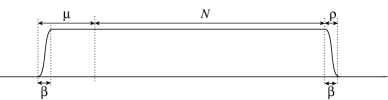
(a) wtx-OFDM and WOLA-OFDM

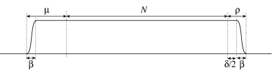
(b) CPW-OFDM

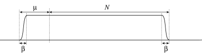
(c) CPwtx-OFDM

Figure 1: Tx windows for different OFDM systems. $N$ is the number subcarriers, $\mu$ is the CP length, $\rho$ is the CS length, $\beta$ is the Tx window tail, and $\delta$ is the Rx window tail.

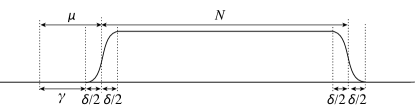
(a) wrx-OFDM and CPW-OFDM

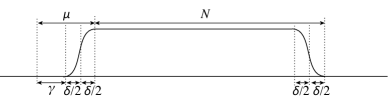
(b) WOLA-OFDM and CPwrx-OFDM

Figure 2: Rx windows for different OFDM systems. $N$ is the number subcarriers, $\mu$ is the CP length, $\gamma$ is the number of samples to be removed, and $\delta$ is the Rx window tail.

Figure 3: Overlap-and-add at the transmitter side.

I-C Contributions

The main contributions in this paper can be summarized as follows:

• A unified formulation for a wide range of OFDM systems is presented. It includes the full transmission chain, the overlap-and-add operation (see Fig. 3), the convolution with a channel of arbitrary length, and the reception process. This compact formulation based on a small set of only six parameters is practical, for instance, for software-defined radio since it allows easy reconfiguration, where different w-OFDM systems are obtained by simply changing the parameter values. In addition, it has excellent potential for use in an educational context, because it enables quickly explaining several OFDM systems under unified expressions.

• Theoretical closed-form expressions of intersymbol and intercarrier interference and noise for the case of an insufficient length of redundant samples are obtained. The interference is identified in the frequency domain, where the symbol is reconstructed, and classified into three different classes. This classification helps to study which class is most harmful to the system’s performance.

• Interference and noise powers are derived to obtain the SINR, and hence the data rate and the symbol-error rate (SER). The resulting expressions are useful for window design, bit-loading, adaptive CP and power/subcarrier allocation algorithms [3].

I-D Organization and Notation

The rest of this paper is organized as follows. In Section II, we present the unified system model, considering seven different OFDM systems and adopting a unified formulation covering all of them. Then, three types of interference are calculated in Section III. In addition, theoretical expressions for both interference and noise powers are derived, and the corresponding SINR is determined. Simulation results are presented in Section IV, and finally, conclusions are drawn in Section V.

The notation used in this paper is as follows. Bold-face letters indicate vectors (lower case) and matrices (upper case). The transpose of ${\bf{A}}$ is denoted by ${\bf{A}}^{T}$ and ${\mathbf{I}}_{N}$ represents the $N\times N$ identity matrix. The subscript is omitted whenever the size is clear from the context. $\mathbf{0}$ and $\mathbf{1}$ denote, respectively, a matrix of zeros or ones.

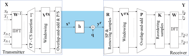
Figure 4: General block diagram of windowed OFDM over a channel with additive noise.

II Unified Formulation

A block diagram is shown in Fig. 4, where the transmitted data vector in the transform domain is given by

$$\mathbf{X}=\left[\begin{array}[]{cccc}X_{0}&X_{1}&\cdots&X_{N-1}\end{array}\right]^{T},$$ (1)

with $N$ being the number of subcarriers. The parameters used in the equations are defined in Table II. We assume perfect synchronization in time and frequency, and also that the receiver has perfect channel-state information (CSI).

II-A Transmitter

The $l$-th time-domain signal vector before the overlap-and-add block is

$$\mathbf{x}_{(N+\mu+\rho)\times 1}^{\rm s}\left[l\right]=\mathbf{V}_{(N+\mu+\rho)}^{\rm tx}\cdot\mathbf{\Gamma}_{(N+\mu+\rho)\times N}\cdot\mathbf{W}_{N}^{-1}\cdot\mathbf{X}_{N\times 1}\left[l\right],$$

where the matrices are defined as follows. First, $\mathbf{W}_{N}^{-1}$ represents the inverse DFT matrix with the $(k,n)$-th entry given by

$$\left[{\bf{W}}_{N}^{-1}\right]_{k,n}=\frac{1}{N}{\rm e}^{{\rm j}\frac{{2\pi}}{N}kn},\quad 0\leq k,n\leq N-1.$$

The matrix $\bf{\Gamma}$ introduces $\mu+\rho$ redundant samples:

$$\bf{\Gamma}=\left[{\begin{array}[]{*{20}c}{\begin{array}[]{*{20}c}{{\bf{0}}_{\mu\times(N-\mu)}}&{{\bf{I}}_{\mu}}\\ \end{array}}\\ {{\bf{I}}_{N}}\\ {\begin{array}[]{*{20}c}{{\bf{I}}_{\rho}}&{{\bf{0}}_{\rho\times({N}-\rho)}}\\ \end{array}}\\ \end{array}}\right].$$

It appends a $\mu$-length CP and, when applicable, also a $\rho$-length CS. Observe that a cyclic shift, as employed in [15], is equivalent to the inclusion of a CS into each data vector. The windowing is represented by the diagonal matrix

$$\mathbf{V}_{(N+\mu+\rho)}^{\rm tx}={\rm diag}\left\{\mathbf{v}_{1\times(N+\mu+\rho)}^{\rm tx}\right\},$$

obtained with a tapering window function, defined as

$$\mathbf{v}_{1\times(N+\mu+\rho)}^{\rm tx}=\left[\begin{array}[]{ccc}\mathbf{v}_{1\times\beta}^{\rm tr}&\mathbf{1}_{1\times(N+\mu+\rho-2\beta)}&\mathbf{v}_{1\times\beta}^{\rm tf}\end{array}\right].$$

The vectors $\mathbf{v}_{1\times\beta}^{\rm tr}$ and $\mathbf{v}_{1\times\beta}^{\rm tf}$ have as entries the rise and fall samples of the window tails, respectively.

After the pulse shaping or windowing, there is a $\beta$-samples overlap-and-add operation between successive symbols , as is depicted in Fig. 3. In the next subsection, this operation is jointly formulated with the channel convolution.

II-B Channel

The signal $\mathbf{x}^{\rm s}$ is convolved with the transmission channel, defined as $\mathbf{h}=\left[\begin{array}[]{cccc}h_{0}&h_{1}&\cdots&h_{\nu}\end{array}\right],$ and becomes contaminated by noise. In general, the number of transmitted data vectors that affect the first $N+\delta+\gamma$ samples of the received data vector is $M+1$, with

$$M\buildrel\Delta\over{=}\left\lceil{\frac{\nu+\beta}{N+\delta+\gamma}}\right\rceil,$$ (2)

in which $\left\lceil\cdot\right\rceil$ represents the ceiling function. Therefore, the $l$-th received signal vector is given by

$${\bf{y}}_{(N+\delta+\gamma)\times 1}^{\rm r} \left[{l}\right]$$

$$=\sum\limits_{m=0}^{M}{{\bf{H}}_{(N+\delta+\gamma)\times(N+\mu+\rho)}^{\left({m}\right)}\cdot{\bf{x}}_{(N+\mu+\rho)\times 1}^{\rm s}\left[{l-m}\right]}$$

$$+{\bf{q}}_{(N+\delta+\gamma)\times 1}[l],$$

where ${\bf{H}}^{(m)}$ is a matrix whose entries, for $0\leq b\leq N+\delta+\gamma-1$ and $0\leq c\leq N+\mu+\rho-1$, are

$$\left[{{\bf{H}}^{(m)}}\right]_{b,c}\buildrel\Delta\over{=}\left\{{\begin{array}[]{*{20}c}{0,}&{mN_{0}+b-c<0,}\\ {h_{mN_{0}+b-c},}&{0\leq mN_{0}+b-c\leq\nu,}\\ {0,}&{mN_{0}+b-c>\nu,}\\ \end{array}}\right.$$ (3)

where $N_{0}=N+\mu+\rho-\beta$ and $\mathbf{q}$ represents the channel noise.

II-C w-OFDM Receiver

The received data vector can be expressed in the transform domain as

$$\mathbf{Y}_{N\times 1}\left[l\right] =\mathbf{W}_{N}\cdot\mathbf{K}_{N}\cdot\mathbf{P}_{N\times(N+\delta)}\cdot\mathbf{V}_{(N+\delta)}^{\rm rx}$$

$$\times\mathbf{R}_{(N+\delta)\times(N+\delta+\gamma)}\cdot\mathbf{y}_{(N+\delta+\gamma)\times 1}^{\rm r}\left[l\right],$$ (4)

where the matrices are defined as follows. First, $\mathbf{R}$ represents removal of the first $\gamma$ samples of the received data vector:

$${\mathbf{R}}=\left[\begin{array}[]{ccc}\mathbf{0}_{(N+\delta)\times\gamma}&\mathbf{I}_{(N+\delta)}\end{array}\right].$$

The diagonal matrix representing the windowing is

$$\mathbf{V}^{\rm rx}={\rm diag}\left\{\mathbf{v}_{1\times(N+\delta)}^{\rm rx}\right\},$$

where the tapering window in the Rx is defined as

$$\mathbf{v}^{\rm rx}=\left[\begin{array}[]{ccc}\mathbf{v}_{1\times\delta}^{\rm rr}&\mathbf{1}_{1\times(N-\delta)}&\mathbf{v}_{1\times\delta}^{\rm rf}\end{array}\right],$$

where $\mathbf{v}^{\rm rr}$ and $\mathbf{v}^{\rm rf}$ have as entries the rise and fall samples of the Rx window tails. Next, $\mathbf{P}$ is a matrix that represents a $\delta$-samples overlap-and-add operation:

$${\bf{P}}=\left[{\begin{array}[]{*{20}c}{\begin{array}[]{*{20}c}{{\bf{0}}_{{\delta\mathord{\left/{\vphantom{\delta 2}}\right.\kern-1.2pt}2}}}&{{\bf{I}}_{{\delta\mathord{\left/{\vphantom{\delta 2}}\right.\kern-1.2pt}2}}}&{{\bf{0}}_{{\delta\mathord{\left/{\vphantom{\delta 2}}\right.\kern-1.2pt}2}\times\left({N-\delta}\right)}}&{{\bf{0}}_{{\delta\mathord{\left/{\vphantom{\delta 2}}\right.\kern-1.2pt}2}}}&{{\bf{I}}_{{\delta\mathord{\left/{\vphantom{\delta 2}}\right.\kern-1.2pt}2}}}\\ \end{array}}\\ {}\hfil\\ {\begin{array}[]{*{20}c}{{\bf{0}}_{\left({N-\delta}\right)\times\delta}}&{{\bf{I}}_{N-\delta}}&{{\bf{0}}_{\left({N-\delta}\right)\times\delta}}\\ \end{array}}\\ {}\hfil\\ {\begin{array}[]{*{20}c}{{\bf{I}}_{{\delta\mathord{\left/{\vphantom{\delta 2}}\right.\kern-1.2pt}2}}}&{{\bf{0}}_{{\delta\mathord{\left/{\vphantom{\delta 2}}\right.\kern-1.2pt}2}}}&{{\bf{0}}_{{\delta\mathord{\left/{\vphantom{\delta 2}}\right.\kern-1.2pt}2}\times\left({N-\delta}\right)}}&{{\bf{I}}_{{\delta\mathord{\left/{\vphantom{\delta 2}}\right.\kern-1.2pt}2}}}&{{\bf{0}}_{{\delta\mathord{\left/{\vphantom{\delta 2}}\right.\kern-1.2pt}2}}}\\ \end{array}}\\ \end{array}}\right].$$

Basically, it adds the first $\delta$ samples to the last $\delta$ samples. Then, a circular shift of $\kappa$ samples is needed in some systems (WOLA, CPwtx, and CPwrx). This operation is formulated with the matrix $\mathbf{K}_{N}$, defined as follows:

$${\bf{K}}_{N}=\left[{\begin{array}[]{*{20}c}{{\bf{0}}_{(N-\kappa)\times\kappa}}&{{\bf{I}}_{N-\kappa}}\\ {{\bf{I}}_{\kappa}}&{{\bf{0}}_{\kappa\times(N-\kappa)}}\\ \end{array}}\right].$$

In some other systems, e.g., those that include a CS in each transmitted data vector (wtx and CPW), this is an identity matrix: $\mathbf{K}_{N}=\mathbf{I}_{N}$. Finally, ${\bf{W}}_{N}$ is a DFT matrix:

$$\left[{\bf{W}}_{N}\right]_{k,n}={\rm e}^{-{\rm j}\frac{{2\pi}}{N}kn},\quad 0\leq k,n\leq N-1.$$

III Analysis of Interference

This section provides a comprehensive analysis of the interference and its power for the considered OFDM systems. Given a finite duration CIR with arbitrary length, without any constraint on the length, the received data vector can be expressed in the transform domain as

$${\bf{Y}}[l]=\sum\limits_{m=0}^{M}{{\bf{A}}_{m}\cdot{\bf{X}}[l-m]}+{\bf{G}}^{\rm noise}\cdot{\bf{q}}[l],$$ (5)

where

$${\bf{A}}_{m,N\times N}=\mathbf{W}\cdot\mathbf{K}\cdot\mathbf{P}\cdot\mathbf{V}^{\rm rx}\cdot\mathbf{R}\cdot{\bf{H}}^{\left(m\right)}\cdot\mathbf{V}^{\rm tx}\cdot\mathbf{\Gamma}\cdot\mathbf{W}^{-1},$$

$${\bf{G}}_{N\times(N+\delta+\gamma)}^{\rm noise}=\mathbf{W}\cdot\mathbf{K}\cdot\mathbf{P}\cdot\mathbf{V}^{\rm rx}\cdot\mathbf{R}.$$

Note that for $\nu\leq\gamma-\beta$, the number of transmitted data vectors affecting the reception (in the transform domain) of a single data vector is one. In this case, a set of $N$ independent parallel subcarriers is obtained, each having a channel gain of $H_{k}$, defined as the $N$-point DFT of the CIR $\bf{h}$. Thus a one-tap per subcarrier equalizer can be used to mitigate the phase and the amplitude distortion introduced by the channel. This means that ${\bf{A}}_{m}=0$, $m>0$, and ${\bf{A}}_{0}$ is a diagonal matrix with elements $H_{k}$, $0\leq k\leq(N-1)$. For the other cases ($\nu>\gamma-\beta$), we have three different types of interference, as depicted in Fig. 5 [40, 38]:

• Type-I intercarrier interference (ICI₁): corresponding to the elements $\left[\mathbf{A}_{0}\right]_{i,j}$, $i\neq j$.

• Type-II intercarrier interference (ICI₂): corresponding to the elements $\left[\mathbf{A}_{m}\right]_{i,j}$, $i\neq j$, $m>0$.

• Intersymbol interference (ISI): corresponding to the diagonal elements $\left[\mathbf{A}_{m}\right]_{i,i}$, $m>0$.

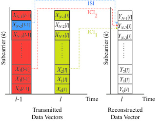
Figure 5: Types of interference.

We now derive theoretical expressions for the powers corresponding to the desired signal component in the received data vector, as well as to the ISI, ICI, and noise. These powers are used to compute the SINR. For this study, we assume that the components of the transmitted data vector $X_{k}$ and the noise vector $q_{k}$ are zero-mean wide-sense stationary uncorrelated processes, independent and identically distributed for all $k$, with variances $\sigma_{X}^{2}$ and $\sigma_{n}^{2}$, respectively.

Let us rewrite (5) as

$${\bf{Y}}[l]={\bf{A}}_{0}\cdot{\bf{X}}[l]+\sum\limits_{m=1}^{M}{{\bf{A}}_{m}\cdot{\bf{X}}[l-m]}+{\bf{G}}^{\rm noise}\cdot{\bf{q}}[l].$$ (6)

The desired signal component in the received data vector can be written as

$$\mathbf{Y}_{{\rm des}}[l]=\mathbf{A}_{0}^{{\rm{des}}}\cdot\mathbf{X}[l],$$ (7)

where ${\mathbf{A}}_{0}^{\rm des}$ is a diagonal matrix with entries $\left[\mathbf{A}_{0}^{{\rm{des}}}\right]_{i,i}=\left[{\mathbf{A}}_{0}\right]_{i,i}.$ The desired signal power (before the transform-domain equalization) at subcarrier $k$ is obtained as the $(k,k)$-th element of the covariance matrix, i.e., $P_{\rm signal}\left(k\right)=\left[{\bf{C}}^{s}\right]_{k,k}$, where

$${\bf{C}}^{s} = E\left\{{\mathbf{Y}_{{\rm des}}[l]\cdot\mathbf{Y}_{{\rm des}}^{H}}[l]\right\}$$ (8)

$$= E\left\{{{\bf{A}}_{0}^{\rm des}\cdot{\bf{X}}[l]\cdot{\bf{X}}^{H}[l]\cdot\left({{\bf{A}}_{0}^{\rm des}}\right)^{H}}\right\}$$

$$= {\bf{A}}_{0}^{\rm des}\cdot E\left\{{\bf{X}}[l]\cdot{\bf{X}}^{H}[l]\right\}\cdot\left({{\bf{A}}_{0}^{\rm des}}\right)^{H}$$

$$= \sigma_{X}^{2}\cdot{\bf{A}}_{0}^{\rm des}\cdot\left({{\bf{A}}_{0}^{\rm des}}\right)^{H},$$

where $E\left\{\cdot\right\}$ is the expected-value operator. The noise data vector is given by

$$\mathbf{Y}_{{\rm noise}}[l]=\mathbf{G}^{\rm noise}\cdot\mathbf{q}[l],$$ (9)

As a result, the noise power is given by $P_{\rm noise}\left(k\right)=\left[{\bf{C}}^{n}\right]_{k,k}$, where

$${\bf{C}}^{n} = {\bf{G}}^{\rm noise}\cdot E\left\{\mathbf{q}[l]\cdot\mathbf{q}^{H}[l]\right\}\cdot\left({{\bf{G}}^{\rm noise}}\right)^{H}$$ (10)

$$= \sigma_{n}^{2}\cdot{\bf{G}}^{\rm noise}\cdot\left({{\bf{G}}^{\rm noise}}\right)^{H}.$$

The interference component is given by

$$\mathbf{Y}_{{\rm int}}[l] = \mathbf{Y}[l]-\mathbf{Y}_{{\rm des}}[l]-\mathbf{Y}_{{\rm noise}}[l]$$ (11)

$$= \mathbf{A}_{0}^{\rm ICI_{1}}\cdot\mathbf{X}[l]+\sum\limits_{m=1}^{M}{\mathbf{A}_{m}\cdot\mathbf{X}[l-m]},$$

where $\mathbf{A}_{0}^{\rm ICI_{1}}=\mathbf{A}_{0}-\mathbf{A}_{0}^{\rm des}$. Using the above, the ISI and ICI power is $P_{{\rm{ISI}},{\rm{ICI}}}\left(k\right)=\left[{\bf{C}}^{i}\right]_{k,k}$, where

$${\bf{C}}^{i} =E\left\{{\mathbf{Y}_{{\rm{int}}}[l]\cdot\mathbf{Y}_{{\rm{int}}}^{H}[l]}\right\}$$

$$=E\left\{{{\bf{A}}_{0}^{{\rm{ICI}}_{\rm{1}}}\cdot{\bf{X}}[l]\cdot{\bf{X}}^{H}[l]\cdot\left({{\bf{A}}_{0}^{{\rm{ICI}}_{\rm{1}}}}\right)^{H}}\right\}$$

$$+\sum\limits_{m=1}^{M}E\left\{{{\bf{A}}_{m}\cdot{\bf{X}}[l-m]\cdot{\bf{X}}^{H}[l-m]\cdot\left({{\bf{A}}_{m}}\right)^{H}}\right\}{\rm{}}$$

$$=\sigma_{X}^{2}\cdot\left({{\bf{A}}_{0}^{{\rm{ICI}}_{\rm{1}}}\cdot\left({{\bf{A}}_{0}^{{\rm{ICI}}_{\rm{1}}}}\right)^{H}+\sum\limits_{m=1}^{M}{{\bf{A}}_{m}\cdot\left({{\bf{A}}_{m}}\right)^{H}}}\right).$$ (12)

Finally, the SINR for subcarrier $k$ is

$${\rm SINR}\left(k\right)=\frac{P_{\rm signal}\left(k\right)}{P_{\rm ISI,ICI}\left(k\right)+P_{\rm noise}\left(k\right)}=\frac{\left[{\bf{C}}^{s}\right]_{k,k}}{\left[{\bf{C}}^{i}\right]_{k,k}+\left[{\bf{C}}^{n}\right]_{k,k}}.$$ (13)

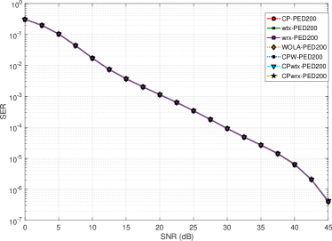
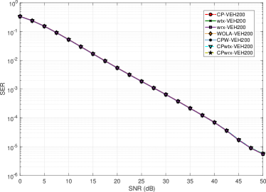
Figure 6: SER versus SNR for different OFDM systems. (a) PED200. (b) VEH200.

TABLE IV: Parameters used in the experiments ($N=256$)

Parameter	CP-OFDM	wtx-OFDM	wrx-OFDM	WOLA-OFDM	CPW-OFDM	CPwtx-OFDM	CPwrx-OFDM
$\beta$	$0$	$8$	$0$	$8$	$8$	$8$	$0$
$\delta$	$0$	$0$	$10$	$10$	$10$	$0$	$10$
$\rho$	$0$	$8$	$5$	$8$	$13$	$0$	$0$
$\gamma$	$32$	$32$	$27$	$22$	$27$	$24$	$22$
$\kappa$	$0$	$0$	$0$	$5$	$0$	$8$	$5$

IV Simulations

In order to demonstrate the applicability of the proposed unified formulation, this section compares the performance of the studied systems in terms of SER and achievable data rate. It is worth noting that OOB emissions will not be taken into account here. The set of parameters used in the simulations are summarized in Table IV. BPSK modulation is used as the primary mapping, the number of active subcarriers is $N=256$, which is the DFT size, and the frequency spacing is $11.16071492$ kHz. Two sets of 250 wireless fading channels each, according to the ITU Pedestrian A and Vehicular A channels [41, 42], are used as multipath channels. They have been generated with Matlab’s stdchan using the channel models itur3GPAx and itur3GVAx with a carrier frequency $f_{\rm c}=2$ GHz and two different sets of parameters: (a) 4 km per hour as pedestrian velocity, $T_{\rm s}=200$ ns and length $L=\nu+1=11$; (b) 100 km per hour as mobile speed, $T_{\rm s}=200$ ns and length $L=\nu+1=21$. These channels are referred to as PED200 and VEH200, respectively. The noise is modeled as an additive white Gaussian noise. It is assumed that the channel remains unchanged within the same simulation and perfect channel estimation is performed at the receiver. Perfect time and frequency synchronization is also assumed.

In Fig. 6, the ${\rm SER}$ performance curves of the different OFDM systems and channels are depicted. As can be seen, the results for the different systems are practically indistinguishable for each set of channels. Thus, there is no clear advantage in terms of SER of any particular OFDM system over the other systems.

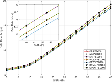
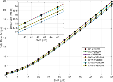
Figure 7: Total achievable data rate versus SNR for different OFDM systems. (a) PED200. (b) VEH200.

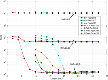
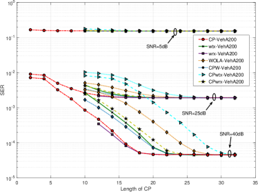
Figure 8: SER versus CP length for different OFDM systems. (a) PED200. (b) VEH200.

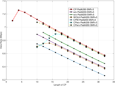
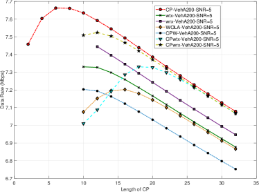
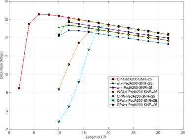
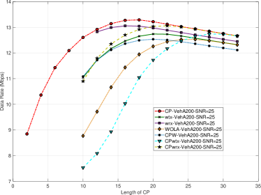
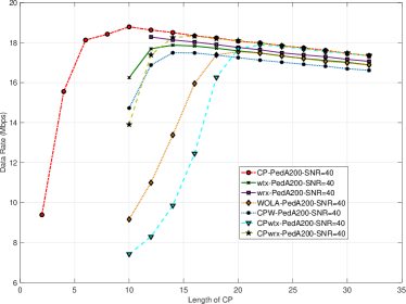
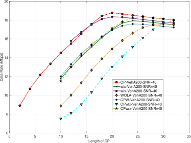
Figure 9: Achievable data rate for different lengths for the CP and SNR values.

Next, we investigate the data rate performance for a fixed CP length ($\mu=32$). As we use BPSK modulation, the data rate for subcarrier $k$ is given by [43]

$$C\left(k\right)=\frac{1}{2}\log_{2}\left({\frac{{{\rm SINR}\left(k\right)}}{\gamma^{\ast}}}\right),$$ (14)

where $\gamma^{\ast}$ is the modified ${\rm SINR}$ gap defined for a target SER as

$$\gamma^{\ast}=\left({\frac{{Q^{-1}\left({{{\rm SER}\mathord{\left/{\vphantom{{\rm SER}2}}\right.\kern-1.2pt}2}}\right)}}{{\sqrt{2}\pi}}}\right)^{2}.$$

The total achievable data rate is thus

$$R=f_{\rm s}\sum\limits_{k=0}^{N-1}{\frac{N}{{N_{0}}}\cdot C\left(k\right)},$$ (15)

where $N_{0}=N+\mu+\rho$ and $f_{\rm s}={1\mathord{\left/{\vphantom{1{T_{\rm s}}}}\right.\kern-1.2pt}{T_{\rm s}}}$. We employ the SER obtained in the previous simulations to compute the values of $\gamma^{\ast}$ corresponding to each SNR. Fig. 7 shows the resulting data rate as a function of the SNR. In this set of experiments, the OFDM systems that offer the best results are CP, wrx and CPwrx. The systems performing windowing in the Rx and including a prefix and suffix, such as WOLA and CPW, offer a lower data rate due to the penalty of adding the two types of redundant samples.

We now analyze the influence of the CP size on the resulting data rate. To this purpose, the SER as a function of the CP length is obtained for each OFDM system (see Fig. 8), assuming ${\rm SNR}=5,25$, and $40$ dB. These results are employed to calculate $\gamma^{\ast}$. Then, we obtain the achievable data rate, depicted in Fig. 9 for the PED200 and VEH200 channels. In all cases, CP-OFDM outperforms the other systems, except for ${\rm SNR}=40$ dB, VEH200, and for smaller values of the CP, for which the wrx-OFDM shows a better performance. However, this improvement is not very significant in this case of insufficient redundant samples. The remaining OFDM systems have better performance whenever the windowing is in the Rx. For both small CP lengths and low SNR values, the systems that only have a CP outperform those that incorporate a CS.

Finally, the formulation presented here allows analysis in the transform domain of the three different interference powers that appear in each OFDM scheme. Fig. 10 shows the total power results ($P_{\rm ICI1}$, $P_{\rm ICI2}$, and $P_{\rm ISI}$) as a function of the CP length, obtained in the previous experiment for the VEH200 channel. The interference power is higher for systems whose windowing is performed in the Tx than those with windowing in the Rx. Note that CPW-OFDM has low levels of interference power, but the data rate results do not outperform the other systems. This is due to the overhead involved in the inclusion of both a CP and CS.

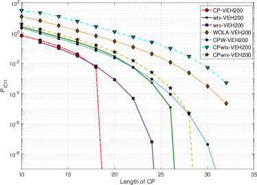
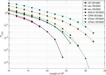
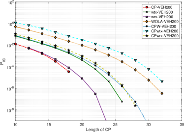
Figure 10: Total power for different CP lengths. (a) Power of type-I intercarrier interference. (b) Power of type-II intercarrier interference. (c) Power of intersymbol interference.

V Conclusion

In this paper, we have presented a unified formulation that describes conventional CP-OFDM and six other different w-OFDM systems. The unified formulation describes the whole transmitter, including the overlap-and-add windowing operation, and the operation of convolving the transmitted signal with the channel, as well as the complete receiver operation. Moreover, we have derived expressions for the intersymbol interference as well as two different kinds of intercarrier interference, along with their corresponding powers, besides the noise component. We have developed analytical expressions for the SINR so as to evaluate the effects of interference on the considered OFDM systems and to study the achievable data rate. Computer simulations have been carried out with practical scenarios. Comparing the obtained results, we have observed that in terms of SER, all OFDM systems behave similarly. However, in terms of data rate, the OFDM systems that only have a windowing in the receiver, or that only include a CP, outperform the other systems. It has also been noted that some systems (such as CPW-OFDM) have low interference power levels, but their data rate performance is slightly lower compared to other systems with more interference. The reason for this can be found in the penalty paid for including both the CP and CS.

References

- [1] J. A. C. Bingham, “Multicarrier modulation for data transmission: An idea whose time has come,” IEEE Communications Magazine, vol. 28, no. 5, pp. 5–14, May 1990.
- [2] Y.-P. Lin, S.-M. Phoong, and P. P. Vaidyanathan, Filter Bank Transceivers for OFDM and DMT systems. Cambridge University Press, 2011.
- [3] J. Cioffi, “Digital communications, chap. 4: Multichannel modulation,” https://web.stanford.edu/group/cioffi/doc/book/chap4.pdf.
- [4] P. S. R. Diniz, W. A. Martins, and M. V. S. Lima, Block Transceivers: OFDM and Beyond. Morgan & Claypool, 2012.
- [5] X. Zhang, L. Chen, J. Qiu, and J. Abdoli, “On the waveform for 5G,” IEEE Communications Magazine, vol. 54, no. 11, pp. 74–80, 2016.
- [6] “Qualcomm inc. - waveform candidates,” Busan, Korea, R1-162199, Apr. 11–15 2016.
- [7] P. Achaichia, M. L. Bot, and P. Siohan, “OFDM/OQAM: A solution to efficient increase the capacity of future PLC networks,” IEEE Trans. on Power Delivery, vol. 26, no. 4, pp. 2443–2455, Oct. 2011.
- [8] F. Cruz-Roldán, F. A. Pinto-Benel, J. Osés del Campo, and M. Blanco-Velasco, “A wavelet OFDM receiver for baseband power line communications,” Journal of the Franklin Institute, vol. 353, no. 7, pp. 1654–1671, May 2016.
- [9] F. A. Pinto-Benel, M. Blanco-Velasco, and F. Cruz-Roldán, “Throughput analysis of wavelet OFDM in broadband power line communications,” IEEE Access, vol. 6, pp. 16 727–16 736, 2018.
- [10] F. A. Pinto-Benel, M. Blanco-Velasco, and F. Cruz-Roldán, “Analysis performance of wavelet OFDM in mobility platforms, Vehicular Communications, vol. 31, 100373, 2021, doi:10.1016/j.vehcom.2021.100373.
- [11] “Data-over-cable service interface specifications Docsis 3.1. Physical layer specification,” CM-SP-PHYv3.1-I07-150910, September 2015.
- [12] “IEEE standard for broadband over power line networks: Medium access control and physical layer specifications,” in IEEE Std 1901-2020 (Revision of IEEE Std 1901-2010), pp.1-1622, 19 Jan. 2021, doi: 10.1109/IEEESTD.2021.9329263.
- [13] “IEEE standard for low-frequency (less than 500 khz) narrowband power line communications for smart grid applications,” IEEE Std 1901.2-2013, September 2013.
- [14] “Unified high-speed wireline-based home networking transceivers - system architecture and physical layer specification,” ITU-T Recommendation G.9960, September 2018.
- [15] “Unified high-speed wireline-based home networking transceivers – multiple input/multiple output specification,” ITU-T Recommendation G.9963, November 2018.
- [16] S. D’Alessandro, A. M. Tonello, and L.Lampe, “Adaptive pulse-shaped OFDM with application to in-home power line communications,” Telecommunication Systems, vol. 51, no. 3-13, September 2012.
- [17] S. H. Müller-Weinfurtner, “Optimum Nyquist windowing in OFDM receivers,” IEEE Transactions on Communications, vol. 49, no. 3, pp. 417–420, 2001.
- [18] R. Zayani, Y. Medjahdi, H. Shaiek, and D. Roviras, “WOLA-OFDM: A potential candidate for asynchronous 5G,” in 2016 IEEE Globecom Workshops (GC Wkshps), pp. 1–5, 2016.
- [19] C. An and H. Ryu, “CPW-OFDM (cyclic postfix windowing OFDM) for the B5G (beyond 5th generation) waveform,” in 2018 IEEE 10th Latin-American Conference on Communications (LATINCOM), pp. 1–4, 2018.
- [20] Y.-P. Lin, C. Li, and S.-M. Phoong, “A filterbank approach to window designs for multicarrier systems,” IEEE Circuits and Systems Magazine, vol. 7, no. 1, pp. 19–30, 2007.
- [21] A. J. Redfern, “Receiver window design for multicarrier communication systems,” IEEE Journal on Selected Areas in Communications, vol. 20, no. 5, pp. 1029–1036, 2002.
- [22] T. Weiss, J. Hillenbrand, A. Krohn, and F. K. Jondral, “Mutual interference in OFDM-based spectrum pooling systems,” in 2004 IEEE 59th Vehicular Technology Conference. VTC 2004-Spring (IEEE Cat. No.04CH37514), vol. 4, pp. 1873–1877, 2004.
- [23] E. Bala, J. Li, and R. Yang, “Shaping spectral leakage: A novel low-complexity transceiver architecture for cognitive radio,” IEEE Vehicular Technology Magazine, vol. 8, no. 3, pp. 38–46, 2013.
- [24] T. Nhan-Vo, K. Amis, T. Chonavel, and P. Siohan, “Achievable throughput optimization in OFDM systems in the presence of interference and its application to power line networks,” IEEE Transactions on Communications, vol. 62, no. 5, pp. 1704–1715, May 2014.
- [25] L. Díez, J. A. Cortés, F. J. Cañete, E. Martos-Naya, and S. Iranzo, “A generalized spectral shaping method for OFDM signals,” IEEE Transactions on Communications, vol. 67, no. 5, pp. 3540–3551, May 2019.
- [26] K. Hussain and R. López-Valcarce, “Joint precoder and window design for OFDM sidelobe suppression,” in IEEE Communications Letters, vol. 26, no. 12, pp. 3044-3048, Dec. 2022, doi: 10.1109/LCOMM.2022.3203521.
- [27] J. Giménez, J. A. Cortés, and L. Díez, “Low-complexity spectral shaping method for OFDM signals with dynamically adaptive emission mask,” IEEE Transactions on Communications, vol. 71, no. 4, pp. 2351–2363, Apr. 2023, doi: 10.1109/TCOMM.2023.3244937.
- [28] B. Peköz, Z. E. Ankarali, S. Köse, and H. Arslan, “Non-redundant OFDM receiver windowing for 5G frames and beyond,” IEEE Transactions on Vehicular Technology, vol. 69, no. 1, pp. 676–684, 2020.
- [29] N. Al-Dhahir and J. M. Cioffi, “Optimum finite-length equalization for multicarrier transceivers,” IEEE Transactions on Communications, vol. 44, no. 1, pp. 56–64, Jan. 1996.
- [30] ——, “A bandwidth-optimized reduced-complexity equalized multicarrier transceiver,” IEEE Transactions on Communications, vol. 45, no. 8, pp. 948–956, Aug. 1997.
- [31] D. Kim and G. L. Stuber, “Residual ISI cancellation for OFDM with applications to HDTV broadcasting,” IEEE Journal on Selected Areas in Communications, vol. 16, no. 8, pp. 1590–1599, Oct. 1998.
- [32] G. Arslan, B. L. Evans, and S. Kiaei, “Equalization for discrete multitone transceivers to maximize bit rate,” IEEE Transactions on Signal Processing, vol. 49, no. 12, pp. 3123–3135, Dec. 2001.
- [33] K. Van Acker, “Equalization and echo cancellation for DMT-based DSL modems,” Ph.D. dissertation, Katholieke Universiteit Leuven, Belgium, 2001.
- [34] W. Henkel, G. Tauböck, P. Ödling, P. O. Börjesson, and N. Petersson, “The cyclic prefix of OFDM/DMT - An analysis,” in Proceedings of 2002 International Zurich Seminar on Broadband Communications. Access, Transmission, Networking, pp. 22–1–22–3, 2002.
- [35] M. Milošević, L. F. C. Pessoa, B. L. Evans, and R. Baldick, “DMT bit rate maximization with optimal time domain equalizer filter bank architecture,” in Thirty-Sixth Asilomar Conference on Signals, Systems and Computers, vol. 1, pp. 377–382, Nov. 2002.
- [36] T. Pham, T. Le-Ngoc, G. K. Woodward, and P. A. Martin, “Channel estimation and data detection for insufficient cyclic prefix MIMO-OFDM,” IEEE Transactions on Vehicular Technology, vol. 66, no. 6, pp. 4756–4768, June 2017.
- [37] B. Lim and Y. C. Ko, “SIR analysis of OFDM and GFDM waveforms with timing offset, CFO, and phase noise,” IEEE Transactions on Wireless Communications, vol. 16, no. 10, pp. 6979–6990, Oct. 2017.
- [38] W. A. Martins, F. Cruz-Roldán, M. Moonen, and P. S. R. Diniz, “Intersymbol and intercarrier interference in OFDM transmissions through highly dispersive channels,” in 2019 27th European Signal Processing Conference (EUSIPCO), pp. 1–5, 2019.
- [39] N. C. Beaulieu and P. Tan, “On the effects of receiver windowing on OFDM performance in the presence of carrier frequency offset,” IEEE Trans. on Wireless Communications, vol. 6, no. 1, pp. 202–209, 2007.
- [40] T. Pollet, H. Steendam, and M. Moeneclaey, “Performance degradation of multi-carrier systems caused by an insufficient guard interval,” in Proceedings of CWAS’97-Intern. Workshop on Copper Wire Access Systems “Bridging the Last Copper Drop”, Budapest, Hungary, pp. 265–270, 27–29 Oct 1997.
- [41] “Guidelines for evaluation of radio transmission technologies for IMT-2000,” ITU, Recommendation ITU-R M.1225, 1997.
- [42] 3rd Generation Partnership Project, 3GPP TS 25.101, Technical Specification Group Radio Radio Access Network. User Equipment (UE) Radio Transmission and Reception (FDD) (Release 7), Sep. 2007.
- [43] A. García-Armada, “SNR gap approximation for M-PSK-based bit loading,” IEEE Transactions on Wireless Communications, vol. 5, no. 1, pp. 57–60, Jan. 2006.