Step Momentum Operator

Abstract

In the present study, the concept of a quantum particle with step momentum is introduced. The energy eigenvalues and eigenfunctions of such particles are obtained in the context of the generalized momentum operator, proposed recently in M.H1 ; M.H2 . While the number of bound states with real energy for the particles with Hermitian step momentum inside a square well is infinite, it is finite for a particle with $\mathcal{PT}$ -symmetric momentum.

I Introduction

After several years of accreditation to Dirac’s definition of Hermitian quantum mechanics, the thought of non-Hermitian systems has been noted by physicists Caliceti . $\mathcal{PT}$-symmetric quantum theory with real energy spectrum has been brought to attention by Bender and Boettcher’s proposal in (Bender1, ) and prospered during the last two decades. A $\mathcal{PT}$-symmetric operator is a non-Hermitian operator which manifests the parity ($\mathcal{P}$) and time-reversal ($\mathcal{T}$) symmetry. We note that $\mathcal{P}$ and $\mathcal{T}$ are defined as $\mathcal{P}x\mathcal{P}=-x$, and $\mathcal{T}i\mathcal{T}=-i$. In a physical approach, a $\mathcal{PT}$-symmetric Hamiltonian is recognized as a gain-loss system being in dynamical equilibrium. Whereas, the time evolution of the corresponding wave function is kept unitary and the continuity equation confirms the conservation of the probability density (MakingSense, ). The other substantial status to take care of is the reality of the eigenvalues. A $\mathcal{PT}$-symmetric system gives real eigenvalues, under the special circumstances, which $\mathcal{PT}$-symmetry of the system is unbroken. However, when the $\mathcal{PT}$-symmetry is broken then the eigenvalues are attained in complex conjugate pairs (MakingSense, ; Dorey, ; BenderBook, ). Mathematically speaking, the domain of space coordinate is broadened to the complex plane as we confront the complex potentials. Thus, the conventional interpretation of inner product in Hilbert space, $\mathcal{H}$, cannot conveniently describe comprehensive dynamical models in non-Hermitian quantum mechanics. To tackle this issue, it is a necessity to amend $\mathcal{H}$, mathematically, in the use of physical systems. To do so, Mostafazadeh in (Mostafazadeh, ) has established the essential definitions in accordance with the pseudo-Hermitian quantum physics which has been organized and reviewed in (Mostafazadeh1, ). In (Mostafazadeh, ; Mostafazadeh1, ), it is indicated that a pseudo-Hermitian Hamiltonian manifests the reality of the spectrum, yet, it is a necessary and sufficient condition for a pseudo-Hermitian operator to be compatible with an invertible and antilinear operator such as $\mathcal{PT}$-symmetric Hamiltonian operator. Hence, $\mathcal{PT}$-symmetry does not guarantee to have real eigenvalues. Accordingly, the pseudo-Hermitian Hamiltonian is introduced as

$$H^{\dagger}\Theta=\Theta H,$$ (1)

in which $\Theta$ is a linear pseudo-metric, positive-definite, Hermitian and invertible operator defined by $\Theta=\Omega^{\dagger}\Omega$, $\Theta:\mathcal{H}\rightarrow\mathcal{H}$. Upon (1) and the definition of $\Theta$ one can modify the inner product

$$\left(\phi,\psi\right)_{\mathcal{H}}=\left\langle\phi\mid\Theta\mid\psi\right\rangle.$$ (2)

this states that $\Omega$ maps $\left|\psi\right\rangle$ from the original Hilbert space $\mathcal{H}$ to the target Hilbert space $\mathcal{L}$ resulting in the Hermitian Hamiltonian- with $\mid\psi\succ=\Omega\left|\psi\right\rangle$, provided $\left|\psi\right\rangle\in\mathcal{H}$ and $\mid\psi\succ\in\mathcal{L}$. Consequently, $H$ in $\mathcal{H}$ corresponds to the constructed Hermitian Hamiltonian $\mathfrak{h}$ in $\mathcal{L}$ defined by (Mostafazadeh, )

$$\mathfrak{h}=\Omega H\Omega^{-1}.$$ (3)

The importance of the Hilbert space modifications and non-Hermitian quantum physics has inspired mathematicians and physicists to investigate extensively in this realm to clarify the ambiguities. Correspondingly, a remarkable triumph is collected in (Znojilbook, ), besides, Znojil has elucidated the alternative approaches of different Hilbert spaces in (Znojil, ).

A non-Hermitian Hamiltonian, i.e, $H\neq H^{\dagger}$, is constituted mostly by the impose of a non-Hermitian potential energy, i.e., $V\left(x\right)\neq V^{*}\left(x\right)$. While the contribution of kinetic energy consistently is unaltered through the exclusivity of the canonical momentum operator, which is Hermitian and by definition, i.e, $p=\frac{\hbar}{i}\frac{d}{dx}$, is $\mathcal{PT}$-symmetric. Moreover, the idea of constructing Hamiltonian using the generalized momentum operator opens the discussion in the context of non-commutative relations associated with the extended uncertainty principle (EUP). We recall that EUP is linked to the existence of minimum momentum (non-commutative1, ). In the virtue of non-Hermitian non-commutative quantum physics, the compatibility of the non-Hermitian operators is discussed in (Znojil-noncom, ), while in (non-commutative2, ) it was shown that how the deformed canonical operators are connected to the non-Hermitian quantum physics. In the recent investigation (non-comm-non-Her, ), the non-Hermitian and non-commutative Hamiltonians are transformed under a set of maps which are proposed based on the implementation of the phase-space formalism.

Here in the present study, we construct a Hermitian step momentum operator as well as its $\mathcal{PT}$-symmetric version in accordance with the recipe presented in (M.H1, ; M.H2, ). Two examples, inspired by the one-dimensional non-Hermitian square well (NSW) potential studied by Znojil in (Znojil1, ; Znojil2, ; Levi-Kovacs, ), are presented. The proposed momentum is founded upon inserting a discrete auxiliary function into the formalism which clarifies the Hermiticity or $\mathcal{PT}$-symmetry of the generalized momentum operator. These examples are considered to be toy models for the more realistic step momentum operator. Let’s add that, classically step momentum implies a particle of constant mass and given velocity, experiencing a change in its velocity in an infinitesimally short time due to an impulsive external force.

This paper is organized as follows. In Sec. II, we present the Hermitian step momentum with the momentum eigenvalue problem. Then, we consider the corresponding Schrödinger equation for a particle in an infinite square well. In Sec. III, we carry out the identical processes for the piece-wise $\mathcal{PT}$-symmetric version of the generalized momentum. Finally in Sec. IV, the outcomes are summarized and compared with the generic canonical momentum operator.

II hermitian step momentum operator

In pursuit of investigating the generalized momentum operator, in accordance with the formalism presented in (M.H1, ), we propose a step Hermitian momentum given by

$$p=-i\hbar\left(1+\mu\left(x\right)\right)\partial_{x}-i\hbar\frac{d\mu\left(x\right)}{2dx}$$ (4)

in which the auxiliary function $\mu\left(x\right)$ is defined to be

$$\mu\left(x\right)=\begin{cases}\mu_{0}&x<0\\ -\mu_{0}&0<x\end{cases},$$ (5)

where $\mu_{0}\in\mathbb{R^{+}}$. Implementing the auxiliary function into Eq. (4) leads to

$$p=\begin{cases}-i\hbar\left(1+\mu_{0}\right)\partial_{x}&x<0\\ -i\hbar\left(1-\mu_{0}\right)\partial_{x}&0<x\end{cases}.$$ (6)

Let’s add that the momentum operator (6) is Hermitian, i.e, $p^{\dagger}=p$ and therefore one expects to attain real eigenvalues, orthogonal eigenfunctions and positive norm. Next, we consider the corresponding eigenvalue equation expressed by

$$p\phi\left(x\right)=\mathfrak{p}\phi\left(x\right)\Rightarrow\begin{cases}-i\hbar\left(1+\mu_{0}\right)\phi_{-}^{\prime}\left(x\right)=\mathfrak{p}\phi_{-}\left(x\right)&x<0\\ -i\hbar\left(1-\mu_{0}\right)\phi_{+}^{\prime}\left(x\right)=\mathfrak{p}\phi_{+}\left(x\right)&0<x\end{cases},$$ (7)

where $\mathfrak{p}$ is the eigenvalue of the eigenfunction $\phi_{\mathfrak{p}}\left(x\right)$ which is found to be

$$\phi_{\mathfrak{p}}\left(x\right)=N\begin{cases}\exp\left(\frac{i\mathfrak{p}x}{\hbar\left(1+\mu_{0}\right)}\right)&x<0\\ 1&x=0\\ \exp\left(\frac{i\mathfrak{p}x}{\hbar\left(1-\mu_{0}\right)}\right)&0<x\end{cases},$$ (8)

in which $N$ stands for the normalization constant. To have the solution physically accepted, $\mathfrak{p}$ has to be real and due to no additional constraint it is continuous.

II.1 Stationary Schrödinger Equation:

Upon applying Eq. (6) into the Hamiltonian operator, one finds the time independent Schrödinger equation in the following form

$$\begin{cases}\frac{-\hbar^{2}}{2m}\left(1+\mu_{0}\right)^{2}\partial_{x}^{2}\psi\left(x\right)+V\left(x\right)\psi\left(x\right)=E\psi\left(x\right)&x<0\\ \frac{-\hbar^{2}}{2m}\left(1-\mu_{0}\right)^{2}\partial_{x}^{2}\psi\left(x\right)+V\left(x\right)\psi\left(x\right)=E\psi\left(x\right)&0<x\end{cases},$$ (9)

where the potential is assumed to be an infinite potential well defined by

$$V(x)=\begin{cases}0&-l<x<l\\ \infty&l\leq|x|\end{cases}.$$ (10)

It is appropriate to rewrite Eq. (9) in the form

$$\begin{cases}\psi\left(x\right)^{\prime\prime}+\kappa^{2}\psi\left(x\right)=0&-l<x<0\\ \psi\left(x\right)^{\prime\prime}+\bar{\kappa}^{2}\psi\left(x\right)=0&0<x<l\end{cases},$$ (11)

where the double prime stands for the second derivative with respect to $x$, $\kappa=\frac{\lambda}{\left(1+\mu_{0}\right)}$ , $\bar{\kappa}=\frac{\lambda}{\left(1-\mu_{0}\right)}$ and $\lambda^{2}=\frac{2mE}{\hbar^{2}}$. Eq. (11) admits a solution expressed as

$$\psi\left(x\right)=\begin{cases}Ae^{i\kappa x}+Be^{-i\kappa x}&-l<x<0\\ Ce^{i\bar{\kappa}x}+De^{-i\bar{\kappa}x}&0<x<l\end{cases},$$ (12)

in which $A,B,C$ and $D$ are integration constant. Next, we apply the boundary and continuity conditions on the solution (12) which lead to

$$\begin{cases}\psi_{-}\left(0\right)=\psi_{+}\left(0\right),\\ \psi_{+}\left(-l\right)=0,\\ \psi_{-}\left(l\right)=0,\\ \partial_{x}\psi_{-}\left(0\right)=\partial_{x}\psi_{+}\left(0\right),\end{cases}\Longrightarrow\begin{cases}A+B-C-D=0\\ Ae^{-i\kappa l}+Be^{i\kappa l}=0,\\ Ce^{i\bar{\kappa}l}+De^{-i\bar{\kappa}l}=0\\ \kappa\left(A-B\right)-\bar{\kappa}\left(C-D\right)=0\end{cases}.$$ (13)

The latter is a homogenous system of four equations with four unknown variables i.e.,$A,B,C$ and $D$. The system admits nontrivial solutions if the determinant of coefficients vanishes. This, however, implies

$$\left|\begin{array}[]{cccc}1&1&-1&-1\\ e^{-i\kappa l}&e^{i\kappa l}&0&0\\ 0&0&e^{i\bar{\kappa}l}&e^{-i\bar{\kappa}l}\\ \kappa&-\kappa&-\bar{\kappa}&\bar{\kappa}\end{array}\right|=0$$ (14)

or explicitly

$$\left(\bar{\kappa}-\kappa\right)\sin l\left(\kappa-\bar{\kappa}\right)+\left(\bar{\kappa}+\kappa\right)\sin l\left(\kappa+\bar{\kappa}\right)=0.$$ (15)

We note that $\kappa$ and $\bar{\kappa}$ contain the energy eigenvalue in accordance with Eq. (11). Hence, one can extract the energy eigenvalues, numerically, using the latter equation. To proceed solving (13) provided $\kappa$ and $\bar{\kappa}$ satisfy the zero determinant condition (15) we introduce $b=\frac{B}{A},c=\frac{C}{A}$ and $d=\frac{D}{A}$ which yields

$$\begin{cases}b-c-d=-1,\\ be^{i\kappa l}=-e^{-i\kappa l},\\ ce^{i\bar{\kappa}l}+de^{-i\bar{\kappa}l}=0,\\ -b\kappa-\bar{\kappa}c+\bar{\kappa}d=-\kappa\end{cases}.$$ (16)

The second equation clearly admits

$$b=-e^{-2i\kappa l}$$ (17)

which upon submitting into the other equations we obtain

$$\begin{cases}c=\frac{\kappa\cos\kappa l}{\bar{\kappa}\cos\bar{\kappa}l}e^{-i\left(\kappa+\bar{\kappa}\right)l}\\ d=-ce^{2i\bar{\kappa}l}\end{cases}.$$ (18)

The main equation which gives the legitimate discrete energy eigenvalues i.e., (15) and identifies the value of the wave numbers $\kappa$ and $\bar{\kappa}$ gives also the constants of integration with respect to $A$. The unknown constant $A$ will be identified using the normalization condition. Let’s introduce $\eta=\lambda l$ and recall the explicit definition of wave numbers which together with equation (15) imply

$$\left(1-\mu_{0}\right)\sin\left(\frac{\eta}{1-\mu_{0}}\right)\cos\left(\frac{\eta}{1+\mu_{0}}\right)+\left(1+\mu_{0}\right)\cos\left(\frac{\eta}{1-\mu_{0}}\right)\sin\left(\frac{\eta}{1+\mu_{0}}\right)=0.$$ (19)

In Fig. 1, we plot the left side of the latter equation in terms of $\eta$ for various values of $\mu_{0}$. Also, in Tab. 1 we present the energy eigenvalues of the first three bound states of the system. We observe that, although, the momentum distribution for negative and positive $x$ axis apparently cancel each other but the energy eigenvalues decrease with increasing $\mu_{0}$. To see the effect of the redistribution of the momentum operator on the probability density we continue to find the explicit form of the wave functions. To do so, we substitute the value of $B=bA,$ $C=cA$ and $D=dA$ in Eq. (12) and after some manipulation and redefinition of the constant $A$, the eigenfunctions are obtained to be

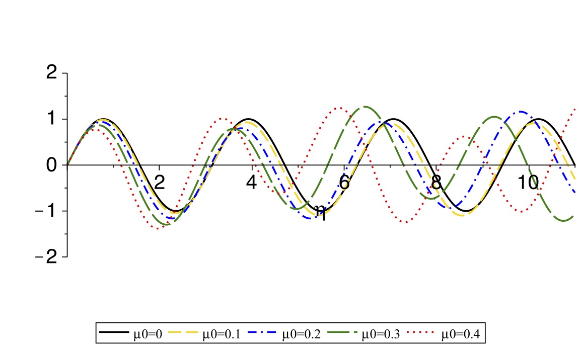
Figure 1: Plot of Eq. (19) with respect to $\eta$ for $\mu_{0}=0$ (solid, black), $\mu_{0}=0.1$ (dash, yellow), $\mu_{0}=0.2$ (dash-dot, blue), $\mu_{0}=0.3$ (long-dash, green) and $\mu_{0}=0.4$ (dot, red). The zero of each curve, corresponds to the $\eta_{n}=\lambda_{n}l$ in which $\lambda_{n}$ gives the allowed energy of the particle. From this figure, we observe that, increasing the value of $\mu_{0}$, decreases the energy of each corresponding state in comparison with $\mu_{0}=0$.

$\mu_{0}$	$0$	$0.1$	$0.2$	$0.3$
$\frac{E_{1}}{E_{0}}$	$1$	$0.9621$	$0.8567$	$0.7112$
$\frac{E_{2}}{E_{0}}$	$4$	$3.9988$	$3.9211$	$3.6181$
$\frac{E_{3}}{E_{0}}$	$9$	$8.6796$	$7.9651$	$7.3006$

Table 1: The relative energy (i.e. $\frac{E_{n}}{E_{0}}$) for $n=1,2$ and $3$ with $\mu_{0}=0.1,0.2$ and $0.3$. Note that $E_{0}$ is the ground state energy of the system with $\mu_{0}=0$.

$$\psi_{n}\left(x\right)=N_{n}\begin{cases}\sin\left(\bar{\kappa_{n}}l\right)\sin\left(\kappa_{n}\left(x+l\right)\right)&-l<x<0\\ -\sin\left(\kappa_{n}l\right)\sin\left(\bar{\kappa_{n}}\left(x-l\right)\right)&0<x<l\end{cases},$$ (20)

in which $N_{n}$ is the normalization constant and the subindex $n=1,2,3,\ldots$ is the state number (the zero-number of (19)) for each given $\mu_{0}$. We would like also to add that the normalization constant $N_{n}$ is function of state. In Fig. 2, we plot the probability density $\left|\psi_{n}\left(x\right)\right|^{2}$ for $n=1,2,3$ with different values of $\mu_{0}=0,0.1,0.2,0.3.$ It is observed that with increasing the value of $\mu_{0}$ the probability distribution changes significantly such that the particle tends to be in the negative $x$-axis. This is reasonable because by increasing $\mu_{0}$ the momentum of the particle for $x<0$ is smaller than for $x>0$ and the particle will have to spend more time in $x<0$.

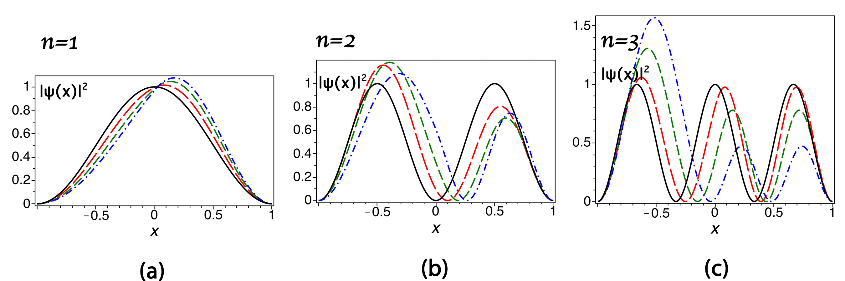
Figure 2: Plots of the probability density of a quantum particle with Hermitian step momentum in the ground, first excited and second excited states in (a), (b), and (c) for $\mu_{0}=0$ (solid, black), $\mu_{0}=0.1$ (long-dash, red), $\mu_{0}=0.2$ (dash, green) and $\mu_{0}=0.3$ (dash-dot, blue).

III $\mathcal{PT}$-Symmetric Step Momentum Operator

In this section, we follow the same steps as of the previous section and introduce a $\mathcal{PT}$-symmetric step momentum operator. To do so, we set the auxiliary function $\mu\left(x\right)$ to be in the form of a finite pure imaginary step function given by

$$\mu(x)=\begin{cases}i\mu_{0}&x<0\\ -i\mu_{0}&0<x\end{cases},$$ (21)

in which $\mu_{0}$ is a positive real value. Inserting the latter equation into Eq. (4) yields a $\mathcal{PT}$-symmetric momentum operator expressed by

$$p=\begin{cases}-i\hbar\left(1+i\mu_{0}\right)\partial_{x}&x<0\\ -i\hbar\left(1-i\mu_{0}\right)\partial_{x}&0<x\end{cases}.$$ (22)

Employing (22), one finds the time-independent Schrödinger equation in the form of

$$\begin{cases}\frac{-\hbar^{2}}{2m}\left(1+i\mu_{0}\right)^{2}\partial_{x}^{2}\psi\left(x\right)+V\left(x\right)\psi\left(x\right)=E\psi\left(x\right)&x<0\\ \frac{-\hbar^{2}}{2m}\left(1-i\mu_{0}\right)^{2}\partial_{x}^{2}\psi\left(x\right)+V\left(x\right)\psi\left(x\right)=E\psi\left(x\right)&0<x\end{cases},$$ (23)

where $E\in\mathbb{R}$ is the energy eigenvalue of the eigenfunction $\psi\left(x\right)$. Our choice of the potential $V\left(x\right)$ is an infinite square well given in Eq. (10). Hence, the Schrödinger equation turns to

$$\begin{cases}\psi\left(x\right)^{\prime\prime}+\kappa^{2}\psi\left(x\right)=0&-l<x<0\\ \psi\left(x\right)^{\prime\prime}+\tilde{\kappa}^{2}\psi\left(x\right)=0&0<x<l\end{cases},$$ (24)

in which $\kappa$ and $\tilde{\kappa}$ are defined to be $\kappa^{2}=\frac{2mE}{\hbar^{2}\left(1+i\mu_{0}\right)^{2}}=\left(s-it\right)^{2}$ and $\tilde{\kappa}^{2}=\frac{2mE}{\hbar^{2}\left(1-i\mu_{0}\right)^{2}}=\left(s+it\right)^{2}$. Introducing a new real parameter

$$\lambda=\sqrt{\frac{2mE}{\hbar^{2}}}\frac{1}{\left(1+\mu_{0}^{2}\right)},$$ (25)

one obtains $s=\lambda$, $t=\lambda\mu_{0}$ and $\tilde{\kappa}$ and $\kappa$ are the complex conjugates of each other. From Eq. (26) we may write

$$E=E_{0}\left(\frac{2\lambda l}{\pi}\right)^{2}\left(1+\mu_{0}^{2}\right)^{2},$$ (26)

with $E_{0}=\frac{\pi^{2}\hbar^{2}}{8ml^{2}}$. The solution to the Schrodinger equation (24) is given by

$$\psi\left(x\right)=\begin{cases}Ae^{i\kappa x}+Be^{-i\kappa x}&-l<x<0\\ Ce^{i\tilde{\kappa}x}+De^{-i\tilde{\kappa}x}&0<x<l\end{cases},$$ (27)

in which $A,B,C$ and $D$ are four integration constants. We note that the boundary conditions for the new configuration, i.e., the $\mathcal{PT}$-symmetric momentum operator other than Hermitian momentum operator, are the same as Eq. (13). Therefore, the similar proceedings in (15) to (16) leads to a constraint equation in terms of $\eta=\lambda l$ expressed by

$$\sin\left(2\eta\right)+\mu_{0}\sinh\left(2\eta\mu_{0}\right)=0.$$ (28)

We would like to add that the complex version of equation (15) admits two constraint equations due to the real and imaginary part of the equation. However, the imaginary part is satisfied trivially due to our assumption of real energy. Eq. (28) is a transcendental equation, therefore, we plot (28) in terms of $\eta$ for several values of $\mu_{0}$ in Fig. 3. The energy eigenvalues are obtained numerically upon applying the zero’s of (28) where the energy of the first three states are expressed in Tab. 2 for $\mu_{0}=0.1,0.2,0.3$. It is observed in Fig. 3 that the number of bound states are finite such that for $\mu_{0}>0.377$ there is no bound state with real energy.

Figure 3: Eq. (28) is plotted in terms of $\eta$, for $\mu_{0}=0$ (solid, black), $\mu_{0}=0.1$ (dash, yellow), $\mu_{0}=0.2$ (dash-dot, blue), $\mu_{0}=0.3$ (long-dash, green), $\mu_{0}=0.4$ (dot, red).

$\mu_{0}$	$0$	$0.1$	$0.2$	$0.3$
$\frac{E_{1}}{E_{0}}$	$1$	$1.0422$	$1.1824$	$1.5035$
$\frac{E_{2}}{E_{0}}$	$4$	$3.9988$	$3.9205$	$3.5791$
$\frac{E_{3}}{E_{0}}$	$9$	$9.4073$	$11.6578$	$-$

Table 2: The relative energy (i.e. $\frac{E_{n}}{E_{0}}$) is presented for $n=1,2$ and $3$ with $\mu_{0}=0.1,0.2$ and $0.3$ for a quantum particle with $\mathcal{PT}$-symmetric step momentum. Note that $E_{0}$ is the ground state energy of the system with $\mu_{0}=0$. The number of states with real energy is finite as for $\mu_{0}=0.3$, there exist merely two bound states.

Following the numerical value for every possible bound state one can in principle find the wave function up to a normalization constant. In terms of $\kappa_{n}$ and $\tilde{\kappa}_{n}$ the wave function is given by

$$\psi_{n}\left(x\right)=N_{n}\begin{cases}\sin\left(\tilde{\kappa_{n}}l\right)\sin\left(\kappa_{n}\left(x+l\right)\right)&-l<x<0\\ \sin\left(\kappa_{n}l\right)\sin\left(\tilde{\kappa_{n}}\left(x-l\right)\right)&0<x<l\end{cases},$$ (29)

in which $N_{n}$ is the normalization constant for the state number $n=1,2,3,\ldots$. We note that $\psi\left(x\right)\psi\left(x\right)^{*}$ is not a probability density when the Hamiltonian is not Hermitian. We refer to Complex correspondence principle where it is indicated that three conditions $\Im\left(\psi\left(x\right)\mathcal{PT}\psi\left(x\right)\right)dx=0$, $\Re\left(\psi\left(x\right)\mathcal{PT}\psi\left(x\right)\right)>0$ and $\int_{C}\left(\psi\left(x\right)\mathcal{PT}\psi\left(x\right)\right)dx=1$, in which $x$ is the complex plane of the particles coordinate. Therefore, instead of $\psi\left(x\right)\psi\left(x\right)^{*}$, $\psi\left(x\right)\mathcal{PT}\psi\left(x\right)$ represents the probability density in complex plane and $\mathbb{C}$ is the specific path where the above conditions are satisfied. Here, it is worth to mention that the $\mathcal{PT}$-symmetric is not exact in this problem. This can be seen clearly if we assume the energy to be complex where we will be able to find the wave function which satisfies all the conditions. In other words, for every specific $\mu_{0}$ there are finite number of bound state with real energy and infinite number of bound states with complex energy. For the sake of comparison, we plot $\left|\psi\left(x\right)\right|^{2}$ in Fig. 4 for the first three bound states with different $\mu_{0}$. The effect of $\mu_{0}$ can be seen as redistribution of $\left|\psi\left(x\right)\right|^{2}$- We also note that $\int\left|\psi\left(x\right)\right|^{2}dx=1$.

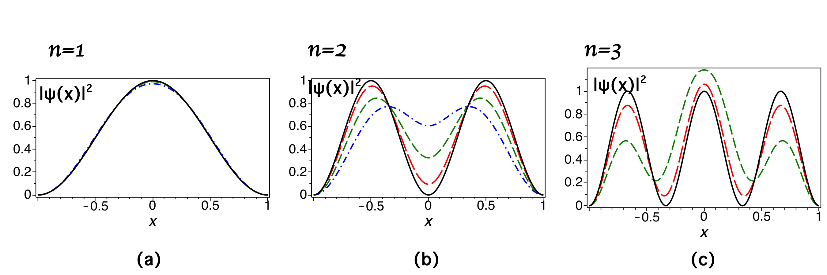
Figure 4: Plots of $\left|\psi\left(x\right)\right|^{2}$- pseudo-probability density- for a quantum particle with $\mathcal{PT}$-symmetric step momentum inside an infinite square well representing the ground, first excited and second excited states which are corresponded to $\mu_{0}=0$ (solid, black), $\mu_{0}=0.1$ (long-dash, red), $\mu_{0}=0.2$ (dash, green) and $\mu_{0}=0.3$ (dash-dot, blue).

III.1 Remark

Here, in this section we intend to find a relation between our outcomes and the results which is acquired in Ref. Znojil1 . M. Znojil, in Ref. Znojil1 , encounters with the ambiguity of continuation of the $\mathcal{PT}$-symmetric square well potential. It is assumed that the energy is real and defined as $E=t^{2}-s^{2}$ with $Z=2st$ to be the measure of non-Hermiticity. However, we rename the latter energy as $E_{z}$ and the energy obtained in the present study $E_{\mu}$, the subindices $Z$ and $\mu$ stand for the factor representing the non-Hermiticity in both studies. Considering $\hbar^{2}=2m=1$, the wave numbers are given by

$$\begin{cases}\kappa_{z}^{2}=E_{z}-iZ,&\kappa_{z}^{*2}=E_{z}+iZ\\ \kappa_{\mu}^{2}=\frac{E_{\mu}}{\left(1+i\mu_{0}\right)^{2}},&\tilde{\kappa}_{\mu}^{2}=\frac{E_{\mu}}{\left(1-i\mu_{0}\right)^{2}}\end{cases}.$$ (30)

Having the identical formulation corresponding to the wave functions in Eq. (12) and Eq. (6) in Znojil1 , we suppose the wave numbers are equal, therefore, from the equality of the latter equations one finds

$$\begin{cases}E_{z}-\frac{\left(1-\mu_{0}^{2}\right)}{\left(1+\mu_{0}^{2}\right)^{2}}E_{\mu}=0\\ Z-\frac{2\mu_{0}}{\left(1+\mu_{0}^{2}\right)^{2}}E_{\mu}=0\end{cases}.$$ (31)

Utilizing equations in (31) with $Z,\mu_{0}>0$, the relationship between $\mu_{0}$ and $Z$ admits

$$\mu_{0}=\frac{E_{z}}{Z}\left(-1+\sqrt{1+\frac{Z^{2}}{E_{z}^{2}}}\right).$$ (32)

The physical approach of the latter comparison indicates that a particle with the $\mathcal{PT}$-symmetric step momentum captured in a standard infinite square well observes an effective potential of the form of $\mathcal{PT}$-symmetric square well. This is due to the corresponding variation in the non-Hermiticity factor in the momentum of the system.

IV Conclusion

Previously, we suggested a structure to form a generalized momentum operator justifying the EUP which is an implication of the minimum momentum. The paradigm was initially concerned with the Hermitian operator M.H1 . Then, we modified the scheme to cover a wider realm upon generating $\mathcal{PT}$-symmetric momentum operator M.H2 . In the present study, we continued the investigation around an exemplar developing a step momentum inspired by the infinite non-Hermitian square well potential Znojil1 . First, we constructed the so-called Hermitian step momentum operator. Its eigenvalue-problem has been solved and the momentum eigenvalues and eigenfunctions have been obtained. The corresponding Schrödinger equation of such particles undergoing an infinite square well has been solved. We plot the probability densities of some of the lower states to see the effect of the main parameter $\mu_{0}$ in the distribution of the particle inside the well. It is observed that the higher the step i. e., $2\mu_{0}$, the more deviated distribution. This redistribution is in a way that the particle tends to stay in the region with a smaller momentum operator which is in agreement with our classical experience. In the second part of the paper, we extended the concept of step momentum and introduced the $\mathcal{PT}$-symmetric step momentum. The energy spectrum of a particle with $\mathcal{PT}$-symmetric momentum inside a square well has been calculated and we have shown that the number of bound states with real energy is finite. Also, it indicates that the $\mathcal{PT}$-symmetry of the system is broken. Besides, we plotted the pseudo-probability density for a few lower states. The plots display the modification of the probability density for $\mu_{0}\neq 0$. We also found that for $\mu_{0}>0.377$ there are no bound states with real energy.

References

-
(1)
E. Caliceti, S. Graffi and M. Maioli, Comm. Math.
Phys. 75, 51(1980);
G. Alvarez, J. Phys. A: Math. Gen. 27, 4589 (1995). - (2) C. M. Bender, S. Boettcher, Phys. Rev. Lett. 80, 5243 (1998).
- (3) C. M. Bender, Rep. Prog. Phys. 70, 947 (2007).
-
(4)
P. Dorey, C. Dunning and R. Tateo, J. Phys. A: Math.
Gen. 34, 391 (2001);
P. Dorey, C. Dunning and R. Tateo, J. Phys. A: Math. Gen. 34, 5679 (2001). - (5) C. Bender, R. Tateo, P. E. Dorey, T. Clare Dunning, G. Levai, S. Kuzhel, H. F. Jones, A. Fring, D. W. Hook, (2018) (London: World Scientific Publishing).
-
(6)
A. Mostafazadeh, J. Math. Phys. 43,
205 (2002);
A. Mostafazadeh, J. Math. Phys. 43, 2814 (2002);
A. Mostafazadeh, J. Math. Phys. 43, 3944 (2002);
A. Mostafazadeh, J. Math. Phys. 44, 974 (2003);
A. Mostafazadeh, J. Phys. A: Math. Gen. 36, 312 (2003); A. Mostafazadeh and A. Batal, J. Phys. A Math. Gen. 37, 11645 (2004); A. Mostafazadeh, Phys. Lett. B 650, 208 (2007);
A. Mostafazadeh, Phys. Scr. 82, 038110 (2010). - (7) A. Mostafazadeh, Int. J. Geom. Methods Mod. Phys. 7, 1191 (2010).
- (8) F. Bagarello, J. P. Gazeau, F. H. Szafraniec and M. Znojil, Eds. J. Wiley & Sons (2015).
-
(9)
M. Znojil, Phys. Rev. D 78, 085003 (2008);
M. Znojil, SIGMA, 5, 1 (2009);
M. Znojil, Acta Polytech. 50, 62 (2010);
M. Znojil, Adv. High Energy Phys. 2018, 7906536 (2018);
M. Znojil, Symmetry, 12, 892 (2020)
M. Znojil, Entropy, 22, 80 (2020). - (10) C. Bambi and F. R. Urban, Class. Quantum Grav. 25, 095006 (2008).
- (11) M. Znojil, I. Semoradova, F. Ruzicka, Phys. Lett. A 95, 042122 (2017).
- (12) B. Bagchi, A. Fring, Phys. Lett. A 373, 4307 (2009).
- (13) J. F. G. dos Santos, F. S. Luiz, O. S. Duarte and M. H. Y. Moussa Eur. Phys. J. Plus, 134, 332 (2019).
- (14) M. Izadparast and S. H. Mazharimousavi, Phys. Scr. 95, 075220 (2020).
- (15) M. Izadparast and S. H. Mazharimousavi, Phys. Scr. 95, 105216 (2020).
- (16) M. Znojil, Phys. Lett. A. 285, 7 (2001).
- (17) M. Znojil, J. Math. Phys. 46, 062109 (2005).
- (18) G. Lévai and J. Kovács, J. Phys. A: Math. Theor. 52, 025302 (2019).
- (19) C. M. Bender, D. W. Hook, P. N. Meisinger and Q. H. Wang, Phys. Rev. Lett. 104, 061601 (2010).