Abstract

We consider interactions of scalar particles, photons, and fermions in Schwarzschild, Reissner-Nordström, Kerr, and Kerr-Newman gravitational and electromagnetic fields with a zero and nonzero cosmological constant. We also consider interactions of scalar particles, photons, and fermions with nonextremal rotating charged black holes in a minimal five-dimensional gauge supergravity. We analyze the behavior of effective potentials in second-order relativistic Schrödinger-type equations. In all cases, we establish the existence of the regime of particle ”falling” on event horizons. An alternative can be collapsars with fermions in stationary bound states without a regime of particles ”falling”.

DOI: 10.1134/S0040577920110070

Keywords: quantum-mechanical hypothesis of cosmic censorship, Schrödinger-type equation, effective potential, scalar particle, photon, fermion, Schwarzschild, Reissner-Nordström, Kerr, and Kerr-Newman black holes with zero and nonzero cosmological constant, anti-de Sitter black hole in five-dimensional supergravity

1 Introduction

For a closed system of ”a particle in an external force field”, quantum mechanics admits the existence of stationary states with certain particle energies. Stationary states include both states of a discrete spectrum (bound states) and states of a continuous spectrum (scattering states). In this case, the particle wave function is written in the form

$$\psi\left({{\rm{\bf r}},t}\right)=\psi\left({{\rm{\bf r}}}\right)e^{-i\,E\,t},$$ (1)

where $E$ is real energy of particle. Here and hereafter, we use the system of units with $\hslash=c=1$.

Here, we consider interactions of scalar particles $\left({S=0}\right)$, photons$\left({S=1}\right)$, and fermions $\left({S=1\mathord{\left/{\vphantom{12}}\right.\kern-1.2pt}2}\right)$ with the Schwarzschild, Reissner-Nordström, Kerr, and Kerr-Newman black holes with a zero and a nonzero cosmological constant. For the listed metrics, we separate the variables in the Klein-Gordon and Maxwell equations. We bring the equations for the radial functions to the form of second-order relativistic Schrödinger-type equations with effective potentials. An analogous procedure was performed using a second-order self-adjoint equation with a spinor wave function for fermions [1]. In addition, we analyze the behavior of effective potentials in neighborhoods of event horizons. We similarly analyze interactions of scalar particles, photons, and fermions with nonextremal rotating charged black holes in a minimal five-dimensional gauge supergravity.

The existence of a regime of particle ”falling” [2], [3] on event horizons was established for all considered metrics and for particles with different spins. Separate states of the considered particles with the energy $E^{ext}$ for extremal black holes and degenerate bound states with $E^{st}$ for fermions are an exception [4] - [6].

For the Schwarzschild, Painlevé -Gullstrand and Kerr metrics, representation (1) was previously used in many papers to prove the existence of nonstationary solutions of the Klein-Gordon and Dirac equations corresponding to bound states of spin and spinless particles with complex energies decaying in time (see, e.g., [7] - [17]). On the other hand, the absence of physically meaningful stationary solutions (with real energy) of the Dirac equation in classical Schwarzschild, Reissner-Nordström, Kerr, and Kerr-Newman fields was proved in [18] - [21].

The presented results are easily explained by the existence of a regime of particles ”falling” on event horizons for all classical black holes, which we proved. As an alternative, the existence of composite systems, collapsars with fermions in degenerate stationary bound states, is possible [4] - [6].

This paper is organized as follows. In Sec. 2, for convenience of analysis, we supplement the quantum mechanical hypothesis of cosmic censorship, previously practically introduced in [22], with numerical characteristics. In more detail, we reveal the content of the regime of a particle ”falling” on a singular center, unacceptable for quantum theory. We show that quantum mechanical hypothesis of cosmic censorship holds in the example of the problem ”Z>137 catastrophe” in hydrogen-like atoms [23]. In Secs. 3 and 4, we study the interaction of scalar particles with Schwarzschild, Painlevé-Gullstrand, Reissner-Nordström, Kerr, and Kerr-Newman black holes with a zero and a nonzero cosmological constant. In Sec. 5, we study this problem for five-dimensional anti-de Sitter black holes. In Secs. 6 and 7, we discuss our results.

We choose the metric signature of the Minkowsky space-time equal to        $\eta_{\alpha\beta}=\mbox{diag}\left[{1,-1,-1,-1}\right]$.

2 Quantum mechanical hypothesis of cosmic censorship

In classical physics, the hypothesis of cosmic censorship, proposed by Penrose [24], forbids the existence in Nature of singularities not covered by event horizons. A quantum mechanical hypothesis of cosmic censorship was practically proposed in [22], in the introduction of which the authors wrote, ”… we will say that a system is nonsingular when the evolution of any state is uniquely defined for all time. If this is not the case, then there is some loss of predictability and we will say that the system is singular”. By analogy with Penrose [24], we must add that such singular systems cannot exist in Nature.

We present some numerical characteristics of singular and nonsingular systems. For second-order radial equations brought to the form of Schrödinger-type equations with effective potentials $U_{eff}\left(\rho\right)$, the behavior of these potentials in neighborhoods of event horizons is important. For all considered metrics, the behavior of effective potentials in neighborhoods of event horizons often has the form of an infinitely deep potential well:

$$\left.{U_{eff}\left(\rho\right)}\right|_{\rho\to\rho_{\pm}}=-\,\frac{K_{1}}{\left({\rho-\rho_{\pm}}\right)^{2}}.$$ (2)

If $K_{1/8}$, then the so-called mode of particle ”falling” on the event horizon occurs [2] - [6]. In this case, the system is singular. The radial function of the Schrödinger-type equation behaves as

$$\left.{R\left(\rho\right)}\right|_{\rho\to\rho_{\pm}}\sim\left({\rho-\rho_{\pm}}\right)^{1/2}\sin\left({\sqrt{K_{2}}\log\left({\rho-\rho_{\pm}}\right)+\delta}\right),$$ (3)

where $K_{2}=2\left({K_{1}-\left({1/8}\right)}\right)$. As $\rho\to\rho_{\pm}$, the radial functions $R\left(\rho\right)$ of stationary states of the discrete and continuous spectra have an infinite number of zeros, and discrete energy levels appear and ”dive” beyond the permitted domains of functions $R\left(\rho\right)$. At $\rho=\rho_{\pm}$, the functions $R\left(\rho\right)$ have no definite values.

The system is also singular if the exponent of the denominator in (2) exceeds two. In this case,

$$\left.{R_{s}\left(\rho\right)}\right|_{\rho\to\rho_{\pm}}\sim\left({\rho-\rho_{\pm}}\right)^{s\mathord{\left/{\vphantom{s4}}\right.\kern-1.2pt}4}\sin\left({\frac{2}{s-2}\sqrt{\frac{K_{1}}{\left({\rho-\rho_{\pm}}\right)^{s-2}}}+\delta_{s}}\right).$$ (4)

In formulas (3) and (4), $\delta$, and $\delta_{s}$ are arbitrary phases $\left({0\leq\delta,\,\,\delta_{s}<\pi}\right)$ and $s>2$ is the exponent in the expression for the effective potential $\left.{U_{eff}\left(\rho\right)}\right|_{\rho\to\rho_{\pm}}=-\,\,{K_{1}}\mathord{\left/{\vphantom{{K_{1}}{\left({\rho-\rho_{\pm}}\right)^{s}}}}\right.\kern-1.2pt}{\left({\rho-\rho_{\pm}}\right)^{s}}$.

If $K_{1}<1/8$ and $s=2$, then the system is nonsingular. In this case, the existence of stationary bound states of particles with $\varepsilon<1_{\,}$ is possible.

In the Hamiltonian formalism, the mode of particle ”falling” on an event horizon corresponds to the fact that the Hamiltonian $H$ has nonzero deficiency indexes [25] - [27]. To eliminate of this mode, we must choose additional boundary conditions on event horizons. A self-adjoint extension of the Hermitian operator $H$ is defined by this choice.

In the history of quantum mechanics, there is an example confirming the quantum mechanical hypothesis of cosmic censorship. For hydrogen-like atoms, the Sommerfeld formula for the fine structure of energy levels has the form

$$\varepsilon=\left({1+\frac{\alpha_{fs}^{2}Z^{2}}{\left({n-\left|\kappa\right|+\sqrt{\kappa^{2}-\alpha_{fs}^{2}Z^{2}}}\right)}}\right)^{-\,1\mathord{\left/{\vphantom{12}}\right.\kern-1.2pt}2},$$ (5)

where $\alpha_{fs}$ is the electromagnetic fine structure constant, $n$ is the principal quantum number, $\kappa$ is the quantum number of the Dirac equation,

$$\kappa=\mp 1,\mp 2,...=\left\{{\begin{array}[]{l}-\left({l+1}\right),\,\,\,\,j=l+\dfrac{1}{2},\\ \,\,\,\,\,\,\,\,\,l,\,\,\,\,\,\,\,\,\,j=l-\dfrac{1}{2},\\ \end{array}}\right.,$$

and $j$ and $l$ are the quantum numbers of the total and orbital angular momentum of a spin -1/2 particle. For $Z>137\left|\kappa\right|$, expression (5) becomes complex (”$Z>137$ catastrophe”).

We consider solutions of a Schrödinger-type equation with an effective potential for fermions in a Coulomb field [28]. The asymptotic formula for the effective potential as $\rho\to 0$ has the form

$$\left.{U_{eff}^{C}}\right|_{\rho\to 0}=-\frac{\left({Z\alpha_{fs}}\right)^{2}-(3/4)+\left({1-\kappa^{2}}\right)}{2\rho^{2}}.$$ (6)

We can distinguish three typical domains depending on Z in asymptotic formula (6). As an example, we consider these domains for the bound states $1S_{1/2}\left({\kappa=-1}\right)$ and $2P_{1/2}\left({\kappa=+1}\right)$. In the first domain $1\leq Z<{\sqrt{3}}\mathord{\left/{\vphantom{{\sqrt{3}}{2\alpha_{fs}}}}\right.\kern-1.2pt}{2\alpha_{fs}}_{\,}$, there exists a positive barrier $\sim 1\mathord{\left/{\vphantom{1{\rho^{2}}}}\right.\kern-1.2pt}{\rho^{2}}_{\,}$ followed by potential well as $\rho\to 0$. The potential barrier disappears at $Z=Z_{cr}={\sqrt{3}}\mathord{\left/{\vphantom{{\sqrt{3}}{2\alpha_{fs}}}}\right.\kern-1.2pt}{2\alpha_{fs}}\approx 118.7$, and the potential well $-K\mathord{\left/{\vphantom{K{\rho^{2}}}}\right.\kern-1.2pt}{\rho^{2}}_{\,}$ persists for $Z>Z_{cr}$ as $\rho\to 0$. In the second domain $119\leq Z<137$, we have the coefficient $K<1/8$, which admits the existence of fermionic stationary bound states [2], [3]. In the third domain $Z\geq 137_{\,}$, there exists a potential well with $K\geq 1/8$ as $\rho\to 0$, which indicates the realization of a regime of ”falling” on the center [2], [3]. We show the dependencies $U_{eff}^{F}\left(\rho\right)$ for $\kappa=-1\left({1S_{1\mathord{\left/{\vphantom{12}}\right.\kern-1.2pt}2}}\right)$ in Fig. 1 for $Z=1,\,119,\,\,140$. We also show the dependencies of the Coulomb potential $V\left(\rho\right)=-\left({{Z\alpha_{fs}}\mathord{\left/{\vphantom{{Z\alpha_{fs}}\rho}}\right.\kern-1.2pt}\rho}\right)$ for comparison.

In the third domain with $\left({Z\alpha_{fs}}\right)^{2}\geq\kappa^{2}$, the system ”fermion in a Coulomb field” is singular. To eliminate the mode of ”falling” on the center, it was proposed to take the finite dimensions of an atomic nucleus into account [29] - [32]. As a result, a cutoff of either the Coulomb or the effective potential occurs at characteristic lengths of the nuclei size (see Fig.1b). There are now about 30 such cutoff methods (see, e.g., [33]).

The system ”an electron in a Coulomb field of an atomic nucleus of finite size” is nonsingular.

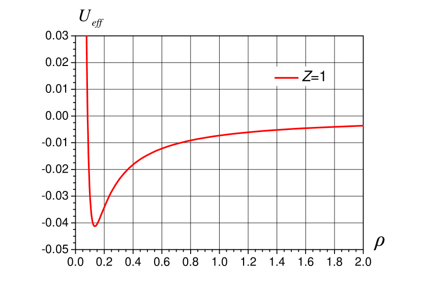
a)

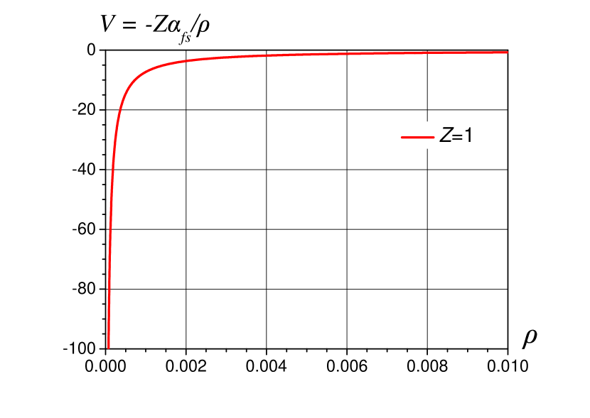
b)

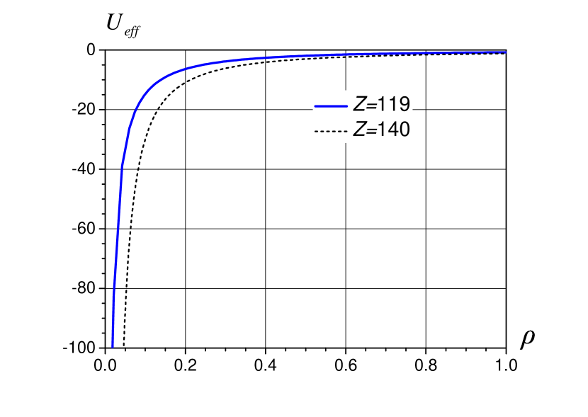
c)

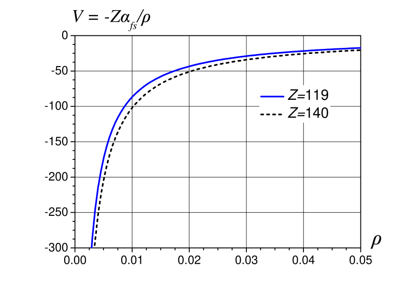
d)

Figure 1: Dependences $U_{eff}\left(\rho\right)$ and $V\left(\rho\right)$: a) $\left.U_{eff}\right|_{\rho\to 0}=-\frac{\left(Z\alpha_{fS}\right)^{2}-(3/4)+\left(1-\kappa^{2}\right)}{2\rho^{2}},\newline \kappa=-1,\,\,\,E/mc^{2}\approx 1$; c) $Z=Z_{cr}=\sqrt{3}/2\alpha_{fs}\approx 118.7,\left.U_{eff}\right|_{\rho\to{0}}=-K/\rho^{2}$.

3 Metrics with a zero cosmological constant

3.1 Brief characteristics of General Relativity solutions and the notation used in the paper

3.1.1 Schwarzschild metric. In the spherical coordinates $\left({t,r,\theta,\varphi}\right)_{\,}$, the Schwarzschild metric has the form

$$ds^{2}=f_{S}dt^{2}-\frac{dr^{2}}{f_{S}}-r^{2}\left({d\theta^{2}+\sin^{2}\theta d\varphi^{2}}\right),$$ (7)

where $f_{S}=1-\left({{r_{0}}\mathord{\left/{\vphantom{{r_{0}}r}}\right.\kern-1.2pt}r}\right)$, $r_{0}={2GM}\mathord{\left/{\vphantom{{2GM}{c^{2}}}}\right.\kern-1.2pt}{c^{2}}$ is the gravitation radius (event horizon), $G$ is the gravitation constant, $M$ is the mass of the gravitational field of a pointlike source, and $c$ is the speed of light.

3.1.2 Painlevé-Gullstrand metric. We write the coordinates as $\left({T,r,\theta,\varphi}\right)$. The coordinate transformation of the Schwarzschild metric in spherical coordinates has the form

$$dT=dt-\sqrt{\frac{r_{0}}{r}}\frac{dr}{{1-r_{0}/r}}.$$ (8)

The interval squared is defined as

$$ds^{2}=f_{S}dT^{2}-2\sqrt{\frac{r_{0}}{r}}dTdr-dr^{2}-r^{2}\left({d\theta^{2}+\sin^{2}\theta d\varphi^{2}}\right).$$ (9)

3.1.3 Reissner-Nordström metric. The static Reissner-Nordström metric is characterized by a pointlike source with a mass $M$ and a charge $Q$:

$$ds^{2}=f_{RN}dt^{2}-\frac{dr^{2}}{f_{RN}}-r^{2}\left({d\theta^{2}+\sin^{2}\theta d\varphi^{2}}\right),$$ (10)

where $f_{RN}=1-r_{0}/r+r_{Q}^{2}/r^{2}$ and $r_{Q}=\sqrt{G}Q/c^{2}$.

If $r_{0}^{2}>4r_{Q}^{2}$, then

$$f_{RN}=\left({1-\frac{\left({r_{+}}\right)_{RN}}{r}}\right)\left({1-\frac{\left({r_{-}}\right)_{RN}}{r}}\right),$$ (11)

where $\left({r_{\pm}}\right)_{RN}$ are the radii of outer and inner event horizons,

$$\left({r_{\pm}}\right)_{RN}=\frac{r_{0}}{2}\pm\sqrt{\frac{r_{0}^{2}}{4}-r_{Q}^{2}}.$$ (12)

The case $r_{0}^{2}=4r_{Q}^{2}$ corresponds to an extremal Reissner-Nordström field with a single event horizon $\left({r_{+}}\right)_{RN}=\left({r_{-}}\right)_{RN}={r_{0}}\mathord{\left/{\vphantom{{r_{0}}2}}\right.\kern-1.2pt}2$.

The case $r_{0}^{2}<4r_{Q}^{2}$ corresponds to a naked singularity. In this case, $f_{RN}>0$.

3.1.4 Kerr and Kerr-Newman metrics. The stationary Kerr-Newman metric is characterized by a pointlike source with the mass $M$ and charge $Q$ rotating with the angular momentum ${\rm{\bf J}}=Mc{\rm{\bf a}}$. The Kerr metrics is the uncharged Kerr-Newman metric $\left({Q=0}\right)$.

We can represent the Kerr-Newman metric in the Boyer-Lindquist coordinates $\left({t,r,\theta,\varphi}\right)_{\,}$ [34] in the form

$$\begin{array}[]{c}ds^{2}=\left({1-\dfrac{r_{0}r-r_{Q}^{2}}{r_{K}^{2}}}\right)dt^{2}+\dfrac{2a\left({r_{0}r-r_{Q}^{2}}\right)}{r_{K}^{2}}\sin^{2}\theta dtd\varphi-\dfrac{r_{K}^{2}}{\Delta_{KN}}dr^{2}-r_{K}^{2}d\theta^{2}-\\[10.0pt] -\left({r^{2}+a^{2}+\dfrac{a^{2}\left({r_{0}r-r_{Q}^{2}}\right)}{r_{K}^{2}}\sin^{2}\theta}\right)\sin^{2}\theta d\varphi^{2},\\ \end{array}$$ (13)

where $r_{K}^{2}=r^{2}+a^{2}\cos^{2}\theta$ and $\Delta_{KN}=r^{2}f_{KN}=r^{2}\left({1-r_{0}/r+\left(r_{Q}^{2}+a^{2}\right)/r^{2}}\right)$.

If $r_{0}>2\sqrt{a^{2}+r_{Q}^{2}}$, then

$$f_{KN}=\left({1-\frac{\left({r_{+}}\right)_{KN}}{r}}\right)\left({1-\frac{\left({r_{-}}\right)_{KN}}{r}}\right),$$ (14)

where $\left({r_{\pm}}\right)_{KN}$ are the radii of outer and inner event horizons of the Kerr-Newman field,

$$\left({r_{\pm}}\right)_{KN}=\frac{r_{0}}{2}\pm\sqrt{\frac{r_{0}^{2}}{4}-a^{2}-r_{Q}^{2}}.$$ (15)

The case $r_{0}=2\sqrt{a^{2}+r_{Q}^{2}},\,\,\,\left({r_{+}}\right)_{KN}=\left({r_{-}}\right)_{KN}={r_{0}}\mathord{\left/{\vphantom{{r_{0}}2}}\right.\kern-1.2pt}2$ corresponds to an extremal Kerr-Newman field.

The case $r_{0}<2\sqrt{a^{2}+r_{Q}^{2}}$ corresponds to a naked singularity of the Kerr-Newman field. In this case, $f_{KN}>0$.

For $Q=0$ , the Kerr-Newman metrics becomes the Kerr metric with

$$\Delta_{K}=r^{2}f_{K}=r^{2}\left({1-\frac{r_{0}}{r}+\frac{a^{2}}{r^{2}}}\right).$$ (16)

If $r_{0}^{2}>4a^{2}$, then

$$f_{K}=\left({1-\frac{\left({r_{+}}\right)_{K}}{r}}\right)\left({1-\frac{\left({r_{-}}\right)_{K}}{r}}\right),$$ (17)

where $\left({r_{\pm}}\right)_{K}=r_{0}/2\pm\sqrt{r_{0}^{2}/4-a^{2}}$.

For $r_{0}=2a$, we have $\left({r_{+}}\right)_{K}=\left({r_{-}}\right)_{K}={r_{0}}\mathord{\left/{\vphantom{{r_{0}}2}}\right.\kern-1.2pt}2$. This case corresponds to an exremal Kerr field.

The case $r_{0}<2a$ corresponds to a naked singularity of the Kerr field. In this case, $f_{K}>0$.

It what follows, we write second-order equations for particles with the energy $E$, mass $m$, and electric charge $q$ in space-time of metrics (7), (9), (10), and (13) in dimensionless variables

$$\begin{array}[]{c}\rho=\dfrac{r}{l_{c}},\,\,\,\varepsilon=\dfrac{E}{mc^{2}},\,\,\,\alpha=\dfrac{r_{0}}{2l_{c}}=\dfrac{GMm}{\hslash c}=\dfrac{Mm}{M_{P}^{2}},\\[10.0pt] \alpha_{Q}=\dfrac{r_{Q}}{l_{c}}=\dfrac{\sqrt{G}Qm}{\hslash c}=\dfrac{\sqrt{\alpha_{fs}}}{M_{P}}m\dfrac{Q}{e},\,\,\,\alpha_{a}=\dfrac{a}{l_{c}},\,\,\,\alpha_{em}=\dfrac{qQ}{\hslash c}=\alpha_{fs}\dfrac{qQ}{e^{2}},\\ \end{array}$$ (18)

where $l_{c}=\hslash\mathord{\left/{\vphantom{\hslash{mc}}}\right.\kern-1.2pt}{mc}$ is the particle Compton wavelength, ${}_{\,}M_{P}=\sqrt{{\hslash c}\mathord{\left/{\vphantom{{\hslash c}G}}\right.\kern-1.2pt}G}=2.2\cdot 10^{-5}\,\,\mbox{g}$    $\left({1.2\cdot 10^{19}\mbox{GeV}}\right)$ is the Planck mass, $\alpha_{fs}={e^{2}}\mathord{\left/{\vphantom{{e^{2}}{\hslash c}}}\right.\kern-1.2pt}{\hslash c}\approx 1\mathord{\left/{\vphantom{1{137}}}\right.\kern-1.2pt}{137}$ is the electromagnetic fine structure constant, $\alpha$ and $\alpha_{em}$ are the gravitational and electromagnetic coupling constants, $\alpha_{Q}$ and $\alpha_{a}$ are dimensionless constants characterizing the electromagnetic field source with the charge $Q$ and the ration of the angular momentum $J$ to the mass $M$ in the Kerr and Kerr-Newman metrics.

For the Kerr-Newman metric, the quantities $\rho_{K}^{2}$ and $\Delta_{KN}$ in the dimensionless variables have the forms

$$\rho_{K}^{2}=\rho^{2}+\alpha_{a}^{2}\cos^{2}\theta,$$ (19)

$$\Delta_{KN}=\rho^{2}f_{KN}=\rho^{2}\left({1-\frac{2\alpha}{\rho}+\frac{\alpha_{a}^{2}+\alpha_{Q}^{2}}{\rho^{2}}}\right).$$ (20)

In the presence of outer and inner event horizons, $\alpha^{2}>\alpha_{a}^{2}+\alpha_{Q}^{2}$, and

$$\left({\rho_{\pm}}\right)_{KN}=\alpha\pm\sqrt{\alpha^{2}-\alpha_{a}^{2}-\alpha_{Q}^{2}}.$$ (21)

For an extremal Kerr-Newman field, $\alpha^{2}=\alpha_{a}^{2}+\alpha_{Q}^{2},\,\,\,\left({\rho_{+}}\right)_{KN}^{ext}=\left({\rho_{-}}\right)_{KN}^{ext}=\alpha,$ and

$$f_{RN}^{ext}=\frac{\left({\rho-\alpha}\right)^{2}}{\rho^{2}}.$$ (22)

For $\alpha^{2}<\alpha_{a}^{2}+\alpha_{Q}^{2}$, the case of a naked singularity of the Kerr-Newman field is realized.

For the Kerr field in formulas (20) and (21), $\alpha_{Q}=0$. For the Reissner-Nordström field in (19) - (21), $\alpha_{a}=0$.

3.2 Motion of scalar particle.

For uncharged particles with zero-spin, the second-order equation in a curved space-time has the form

$$\left({-g}\right)^{{-1}\mathord{\left/{\vphantom{{-1}2}}\right.\kern-1.2pt}2}\frac{\partial}{\partial x^{\mu}}\left[{\left({-g}\right)^{1\mathord{\left/{\vphantom{12}}\right.\kern-1.2pt}2}g^{\mu\nu}\frac{\partial}{\partial x^{\nu}}\Phi}\right]+m^{2}\Phi=0,$$ (23)

where $g$ is the determinant of the metric. After separation of variables, the equation for the radial function $R\left(\rho\right)$ becomes

$$\frac{d^{2}R}{d\rho^{2}}+A\left(\rho\right)\frac{dR}{d\rho}+B\left(\rho\right)R=0,$$ (24)

where $\rho=r\mathord{\left/{\vphantom{r{l_{c}}}}\right.\kern-1.2pt}{l_{c}}$.

We bring Eq. (24) to the form of a Schrödinger equation with the effective potential $U_{eff}\left(\rho\right)$:

$$\bar{{R}}_{l}\left(\rho\right)=R\left(\rho\right)\exp\left[\frac{1}{2}\int{A\left({{\rho}^{\prime}}\right)}d{\rho}^{\prime}\right],$$ (25)

$$\frac{d^{2}\bar{{R}}\left(\rho\right)}{d\rho^{2}}+2\left({E_{Schr}-U_{eff}\left(\rho\right)}\right)\bar{{R}}\left(\rho\right)=0,$$ (26)

$$U_{eff}\left(\rho\right)=E_{Schr}+\frac{1}{4}\frac{dA}{d\rho}+\frac{1}{8}A^{2}-\frac{1}{2}B,$$ (27)

$$E_{Schr}=\frac{1}{2}\left({\varepsilon^{2}-1}\right).$$ (28)

The term $E_{Schr}$ given by (28) is distinguished in Eq. (26) and at the same time added to (27). This is done, on one hand, to give Eq. (26) the form of a Schrödinger-type equation and, on the other hand, to ensure the classical asymptotic form of the effective potential as $\rho\to\infty$.

3.2.1 Kerr and Kerr-Newman metrics. In this section, we use results in [35], where variables in Eq. (23) were separates for the Kerr and Kerr-Newman metrics and for uncharged scalar particles.

In dimensionless variables (18), the wave function has the form

$$\Phi_{KN}\left({{\rm{\bm{\rho}}},t}\right)=R_{KN}\left(\rho\right)S\left(\theta\right)e^{-i\varepsilon t}e^{i\,m_{\varphi}\,\varphi},$$ (29)

where $S\left(\theta\right)$ are oblate spheroidal harmonic functions $S_{lm_{\varphi}}\left({ic,\cos\theta}\right)$, $c^{2}=\alpha_{a}^{2}\left({\varepsilon^{2}-1}\right)$, and $l$ and $m_{\varphi}\,$ are the quantum numbers of the orbital momentum and its projection $\left({\left|{m_{\varphi}}\right|\leq l}\right)$.

The equations of the radial functions have the form [35]

$$\begin{array}[]{c}\dfrac{d}{d\rho}\left({\Delta_{KN}\dfrac{dR_{KN}}{d\rho}}\right)+\dfrac{1}{\Delta_{KN}}\left[{\varepsilon^{2}\left({\rho^{2}+\alpha_{a}^{2}}\right)^{2}-2\left({2\alpha\rho-\alpha_{Q}^{2}}\right)\varepsilon\alpha_{a}m_{\varphi}+m_{\varphi}^{2}\alpha_{a}^{2}-}\right.\\[10.0pt] \left.{-\left({\varepsilon^{2}\alpha_{a}^{2}+\rho^{2}+\lambda_{lm_{\varphi}}^{KN}}\right)\Delta_{KN}}\right]R_{KN}=0,\\ \end{array}$$ (30)

where $\lambda_{lm_{\varphi}}^{KN}\left({\alpha_{a},\varepsilon}\right)$ is the separation constant for Eq. (23). In accordance with (24) - (28), for Eq. (30), we can write

$$\begin{array}[]{c}A_{KN}=\dfrac{2\left({\rho-\alpha}\right)}{\Delta_{KN}},\\[10.0pt] B_{KN}=\dfrac{1}{\Delta_{KN}^{2}}\left\{{\left[{\varepsilon\left({\rho^{2}+\alpha_{a}^{2}}\right)-\alpha_{a}m_{\varphi}}\right]^{2}-\left({\varepsilon^{2}\alpha_{a}^{2}-2\varepsilon\alpha_{a}m_{\varphi}}\right)\Delta_{KN}-\left({\rho^{2}+\lambda_{lm_{\varphi}}^{KN}}\right)\Delta_{KN}}\right\}.\end{array}$$ (31)

In explicit form, the effective potential $U_{eff}^{KN}\left(\rho\right)$ in the Schrödinger-type equation with (27) and (31) taken into account is

$$\begin{array}[]{c}U_{eff}^{KN}\left(\rho\right)=\dfrac{1}{2}\left({\varepsilon^{2}-1}\right)+\dfrac{1}{2\Delta_{KN}}+\dfrac{\varepsilon^{2}\alpha_{a}^{2}-2\varepsilon\alpha_{a}m_{\varphi}}{2\Delta_{KN}}+\dfrac{\rho^{2}}{2\Delta_{KN}}+\dfrac{\lambda_{lm_{\varphi}}^{KN}}{2\Delta_{KN}}-\\[10.0pt] -\dfrac{\left({\rho-\alpha}\right)^{2}}{2\Delta_{KN}^{2}}-\dfrac{1}{2\Delta_{KN}^{2}}\left[{\varepsilon\left({\rho^{2}+\alpha_{a}^{2}}\right)-\alpha_{a}m_{\varphi}}\right]^{2}.\\ \end{array}$$ (32)

3.2.2 Asymptotic behavior of the effective potential. As $\rho\to\infty$, we have

$$\left.{U_{eff}^{KN}}\right|_{\rho\to\infty}=\,\frac{\alpha}{\rho}\left({1-2\varepsilon^{2}}\right)+{\rm O}\left({\frac{1}{\rho^{2}}}\right).$$ (33)

As $\rho\to 0$,

$$\left.{U_{eff}^{KN}}\right|_{\rho\to 0}\to\mbox{const}_{KN}+{\rm O}\left(\rho\right).$$ (34)

As $\rho\to\left({\rho_{\pm}}\right)_{KN}$,

$$\left.{U_{eff}^{KN}}\right|_{\rho\to\left({\rho_{\pm}}\right)_{KN}}=-\,\,\frac{1}{\left({\rho-\left({\rho_{\pm}}\right)_{KN}}\right)^{2}}\left\{{\frac{1}{8}+\frac{\left[{\varepsilon\left({\left({\rho_{\pm}}\right)_{KN}^{2}+\alpha_{a}^{2}}\right)-\alpha_{a}m_{\varphi}}\right]^{2}}{2\left({\left({\rho_{+}}\right)_{KN}-\left({\rho_{-}}\right)_{KN}}\right)^{2}}}\right\}.$$ (35)

For the Kerr metric, asymptotic formulas (33) - (35) hold with $\alpha_{Q}=0$. The asymptotic formulas for the Reissner-Nordström metric can be obtained from (33) and (35) with $\alpha_{a}=0$. The asymptotic formulas for the Schwarzschild metric are obtained from (33) and (35) with $\alpha_{a}=0$ and $\alpha_{Q}=0$. Asymptotic formula (35) indicates that the systems ”a scalar particle in Kerr, Kerr-Newman, Reissner-Nordström, and Schwarzschild fields” are singular.

3.2.3 Painlevé-Gullstrand metric in the coordinates $\left({\bf T,r,\bm{\theta},\bm{\varphi}}\right)$. The stationary Eddington-Finkelstein [36], [37] and Painlevé-Gullstrand [38], [39] metrics and the nonstationary Lemaître -Finkelstein [40], [37] and Kruskal-Szekeres [41], [42] metrics were previously obtained by coordinate transformation of the Schwarzschild metric (7) to eliminate the singularity on the event horizon $r_{0}$. But in quantum mechanics, the singularity for all mentioned metrics is manifested in the final results. In [43], this was shown in the example of a spin-1/2 particle, and the equivalence of the Schwarzschild metric and metrics indicated above was shown for the regular solution $\varepsilon=0$. In this section, for the Painlevé -Gullstrand metric, we see the same behavior of the effective potential in a neighborhood of $\rho=2\alpha$ and $\rho\to\infty$ as for the Schwarzschild metric in Sec. 3.2.2 (see (33), (35)) for $\alpha_{a}=0$ and $\alpha_{Q}=0$).

In accordance with (9), $\sqrt{-g}=r^{2}\sin\theta$,

$$g^{00}=1,\,\,\,g^{01}=g^{10}=-\sqrt{\frac{r_{0}}{r}},\,\,\,g^{11}=-f_{S},\,\,g^{22}=-\frac{1}{r^{2}},\,\,\,g^{33}=-\frac{1}{r^{2}\sin^{2}\theta}.$$

We present the wave function $\Phi_{PG}\left({{\rm{\bf r}},T}\right)$ for stationary states in the form

$$\Phi_{PG}\left({{\rm{\bf r}},T}\right)=P_{l}\left(r\right)Y_{lm_{\varphi}}\left({\theta,\varphi}\right)e^{-iET}.$$ (36)

After separation of variables in (23) and substitution (36), the equations for the radial functions $P_{l}\left(r\right)$ become

$$\begin{array}[]{c}\dfrac{d^{2}P_{l}}{dr^{2}}+\left({\dfrac{1}{r^{2}}\left({2r-r_{0}}\right)-i2\sqrt{\dfrac{r_{0}}{r}}E}\right)\dfrac{1}{f_{S}}\dfrac{dP_{l}}{dr}+\\[10.0pt] +\left[{\dfrac{\left({E^{2}-m^{2}}\right)}{f_{S}}-\dfrac{l\left({l+1}\right)}{r^{2}f_{S}}-\dfrac{iE}{r^{2}f_{S}}\sqrt{\dfrac{r_{0}}{r}}\left({2r-\dfrac{r_{0}}{2}}\right)}\right]P_{l}=0.\end{array}$$ (37)

By analogy with Eq. (24), after passing to dimensionless variables (18), we define

$$\begin{array}[]{l}A_{PG}=\dfrac{1}{f_{S}}\left({\dfrac{2\left({\rho-\alpha}\right)}{\rho^{2}}-i2\varepsilon\sqrt{\dfrac{2\alpha}{\rho}}}\right),\\[10.0pt] B_{PG}=\frac{1}{f_{S}}\left({\varepsilon^{2}-1}\right)-\dfrac{1}{\rho^{2}f_{S}}l\left({l+1}\right)-i\varepsilon\dfrac{1}{\rho^{2}f_{S}}\sqrt{\dfrac{2\alpha}{\rho}}\left({2\rho-\alpha}\right).\end{array}$$ (38)

Further, we bring Eq. (37) to the form of a Schrödinger equation with the effective potential $U_{eff}^{PG}\left(\rho\right)$:

$$\begin{array}[]{l}\bar{{P}}_{l}\left(\rho\right)=P_{l}\left(\rho\right)\exp\left[\dfrac{1}{2}\int{A_{PG}\left({{\rho}^{\prime}}\right)}d{\rho}^{\prime}\right],\\[10.0pt] \dfrac{d^{2}\bar{{P}}_{l}\left(\rho\right)}{d\rho^{2}}+2\left({E_{Schr}-U_{eff}^{PG}\left(\rho\right)}\right)\bar{{P}}_{l}\left(\rho\right)=0,\\[10.0pt] U_{eff}^{PG}\left(\rho\right)=E_{Schr}+\dfrac{1}{4}\dfrac{dA_{PG}}{d\rho}+\dfrac{1}{8}A_{PG}^{2}-\dfrac{1}{2}B_{PG},\\[10.0pt] E_{Schr}=\frac{1}{2}\left({\varepsilon^{2}-1}\right).\end{array}$$ (39)

An explicit formula for $U_{eff}^{PG}\left(\rho\right)$ is given in Appendix A. Equalities (37) - (39) are complex. But analysis of the asymptotic behavior of $U_{eff}^{PG}\left(\rho\right)$ shows that the leading singularities are on the real axis and completely coincide with the singularities for the Schwarzschild metric. Therefore, the system ”a scalar particle in the Painlevé -Gullstrand field” is singular. Obviously, we can also draw the same conclusion for the stationary Eddington-Finkelstein metric [36], [37].

3.2.4 Extremal Kerr and Kerr-Newman fields. In the case of the extremal Kerr and Kerr-Newman fields, there exists a single event horizon $\rho=\alpha$. Moreover, $\alpha^{2}=\alpha_{a}^{2}+\alpha_{Q}^{2}$ and $\Delta_{KN}=\left({\rho-\alpha}\right)^{2}$.

The expression for effective potential (32) becomes

$$\begin{array}[]{c}U_{eff}^{ext}=\dfrac{1}{2}\left({\varepsilon^{2}-1}\right)+\dfrac{\rho^{2}}{2\left({\rho-\alpha}\right)^{2}}+\frac{\lambda_{ext}}{2\left({\rho-\alpha}\right)^{2}}+\dfrac{\varepsilon^{2}\alpha_{a}^{2}-2\varepsilon\alpha_{a}m_{\varphi}}{2\left({\rho-\alpha}\right)^{2}}-\\[10.0pt] -\dfrac{\left({\rho^{2}+\alpha_{a}^{2}}\right)^{2}}{2\left({\rho-\alpha}\right)^{4}}\left({\varepsilon-\dfrac{\alpha_{a}m_{\varphi}}{\rho^{2}+\alpha_{a}^{2}}}\right)^{2}.\end{array}$$ (40)

As $\rho\to\infty$, the asymptotic formula for $U_{eff}^{ext}$ remains as in (33). As $\rho\to 0$, we must take the equality $\alpha^{2}=\alpha_{a}^{2}+\alpha_{Q}^{2}$ into account in $\mbox{const}_{KN}$ in asymptotic formula (34) . As $\rho\to\alpha$ and under the condition that $\varepsilon\neq\varepsilon^{ext}=\alpha_{a}m_{\varphi}/(\alpha^{2}+\alpha_{a}^{2})$, the effective potential has the form

$$\left.{U_{eff}^{ext}}\right|_{\rho\to\alpha}=-\,\frac{\left({\alpha^{2}+\alpha_{a}^{2}}\right)^{2}}{2\left({\rho-\alpha}\right)^{4}}\left({\varepsilon-\varepsilon^{ext}}\right)^{2}+{\rm O}\left({\frac{1}{\left({\rho-\alpha}\right)^{2}}}\right).$$ (41)

As $\rho\to\alpha$ and for $\varepsilon=\varepsilon^{ext}$, we can write the expression for $U_{eff}^{ext}$ as

$$\left.{U_{KN}^{ext}\left({\varepsilon=\varepsilon^{ext}}\right)}\right|_{\rho\to\alpha}=\frac{1}{2\left({\rho-\alpha}\right)^{2}}\left[{C_{ext}+\lambda_{ext}+\alpha^{2}-\Omega^{2}}\right],$$ (42)

where

$$C_{ext}=\varepsilon^{ext}\alpha_{a}\left({\varepsilon^{ext}-2\alpha m_{\varphi}}\right),\,\,\,\,\,\Omega=\frac{2\alpha\alpha_{a}m_{\varphi}}{\left({\alpha^{2}+\alpha_{a}^{2}}\right)}.$$ (43)

If

$$C_{ext}+\lambda_{ext}+\alpha^{2}-\Omega^{2}>0$$ (44)

in (42), then there exists a potential barrier on the event horizon. If $C_{ext}+\lambda_{ext}+\alpha^{2}-\Omega^{2}\geq 3/4$, then the barrier becomes quantum mechanically impenetrable.

If

$$-\dfrac{1}{4}<C_{ext}+\lambda_{ext}+\alpha^{2}-\Omega^{2}<0,$$ (45)

then there exists a potential well near the event horizon, and in this case, the stationary bound state of scalar particles with $\varepsilon=\varepsilon^{ext}$ can exist in domains of the wave functions $\rho\in\left[{\alpha,\infty}\right)$ and $\rho\in\left({0,\alpha}\right]$.

If

$$C_{ext}+\lambda_{ext}+\alpha^{2}-\Omega^{2}\leq-\dfrac{1}{4},$$ (46)

then the regime of particles ”falling” on the event horizon is realized.

For $\varepsilon\neq\varepsilon^{ext}$, in accordance with asymptotic formula (41), the systems ”a scalar particle in an extremal Kerr and Kerr-Newman field” are singular. For $\varepsilon=\varepsilon^{ext}$, the systems are singular if inequality (46) is satisfied.

3.3 Photon in gravitational and electromagnetic fields of asymptotically flat vacuum solutions of General Relativity

3.3.1 Photon in a Kerr field. Teukolsky [45] separated the variables in the Maxwell equations in a Kerr space-time [44] (also see (13), (16), (17)). The function $\psi$ of the master equation was presented in the form

$$\psi=e^{-i\omega\,t}e^{im\,\,\varphi}S\left(\theta\right)R\left(r\right).$$ (47)

The function $\psi$ in [45] is related to the components of the electromagnetic field tensor convoluted with components of the Kinnersley tetrad [46] in the Newman-Penrose formalism [47]. For our analysis, the Teukolsky separation of variables has a significant disadvantage: the equation for the radial function $R\left(r\right)$ and hence also the effective potential in the Schrödinger equation are complex.

Lunin [48] introduced new more complicated relation of ansatz (47) to the components of the electromagnetic field potential $A^{\mu}\left({{\rm{\bf r}},t}\right)$. As a result, a separation of variables with a real equation for the radial function $R\left(r\right)$ was produced. In the Lunin terminology, variables are separated for the ”electric polarization” and for the ”the magnetic polarization” (Teukolsky did not separate the variables for ”the magnetic polarization”). For a better understanding, we write the final formulas from [48].

The electrical polarization is described by the relations

$$\begin{array}[]{c}l_{\pm}^{\mu}A_{\mu}^{\left({el}\right)}=\pm\dfrac{r}{1\pm i\mu r}\hat{{l}}_{\pm}\Psi,\,\,\,\,\,m_{\pm}^{\mu}A_{\mu}^{\left({el}\right)}=\mp\dfrac{iac_{\theta}}{1\pm i\mu ac_{\theta}}\hat{{m}}_{\pm}\Psi,\,\,\,\,\Psi=e^{-i\,\omega\,t+i\,m\,\,\varphi}R\left(r\right)S\left(\theta\right),\\[10.0pt] \dfrac{E_{\theta}}{s_{\theta}}\dfrac{d}{d\theta}\left[{\dfrac{s_{\theta}}{E_{\theta}}\dfrac{d}{d\theta}S}\right]+\left\{{-\dfrac{2\Lambda}{E_{\theta}}+\left({a\omega c_{\theta}}\right)^{2}-\dfrac{m^{2}}{s_{\theta}^{2}}-C}\right\}S=0,\\[10.0pt] E_{r}\dfrac{d}{dr}\left[{\dfrac{\Delta_{K}}{E_{r}}\dfrac{d}{dr}R}\right]+\left\{{\dfrac{2\Lambda}{E_{r}}+\left({\omega r}\right)^{2}+\dfrac{\left({am}\right)^{2}}{\Delta_{K}}+\dfrac{r_{0}r\omega^{2}\Delta_{0}}{\Delta_{K}}-\dfrac{2r_{0}ar\omega m}{\Delta_{K}}+C}\right\}R=0,\\ \end{array}$$ (48)

where $E_{r}=1+\left({\mu r}\right)^{2},\,\,\,E_{\theta}=1-\left({\mu ac_{\theta}}\right)^{2},\,\,\,\Delta_{K}=r^{2}+a^{2}-r_{0}r,\,\,\,\Delta_{0}=r^{2}+a^{2},\,\,s_{\theta},\,\,c_{\theta}=\sin\theta,\newline \cos\theta,\,\,\,\xi=a\mu\left[{m-a\omega+\omega/a\mu^{2}}\right],\,\,\,C=-\xi-2am\omega+\left({a\omega}\right)^{2}$, $\mu$ is the separation constant,

$$\begin{array}[]{c}l_{+}^{\mu}=l^{\mu},\,\,\,\,\,l_{-}^{\mu}=-2\rho_{k}^{2}n^{\mu}/\Delta_{K},\\[10.0pt] m_{+}^{\mu}=\sqrt{2}\rho m^{\mu},\,\,\,\,m_{-}^{\mu}=\sqrt{2}\rho^{\ast}m^{\ast\mu},\,\,\,\,\,\rho=r+ia\cos\theta,\\[10.0pt] l_{\pm}^{\mu}\partial_{\mu}=\partial_{r}\pm\left[{\dfrac{r^{2}+a^{2}}{\Delta_{K}}\partial_{t}+\dfrac{a}{\Delta_{K}}\partial_{\varphi}}\right],\,\,\,\,\,\,m_{\pm}^{\mu}\partial_{\mu}=\partial_{\theta}\pm\left[{ia\sin\theta\,\partial_{t}+\dfrac{i}{\sin\theta}\partial_{\varphi}}\right],\\[10.0pt] \end{array}$$ (49)

$l^{\mu},\,\,n^{\mu},\,\,m^{\mu}$, and $m^{\ast\mu}$ are components of the Kinnersley tetrad vectors [46] with $l_{\mu}n^{\mu}=-1$ and $m_{\mu}m^{\ast\mu}=1$.

The magnetic polarization is described by the formulas

$$\begin{array}[]{c}l_{\pm}^{\mu}A_{\mu}^{\left({mgn}\right)}=\pm\dfrac{ia}{1\pm i\mu a}\hat{{l}}_{\pm}\Psi,\,\,\,\,\,m_{\pm}^{\mu}A_{\mu}^{\left({mgn}\right)}=\mp\dfrac{1}{c_{\theta}\mp\mu}\hat{{m}}_{\pm}\Psi,\,\,\,\,\,\Psi=e^{-i\,\omega\,t+i\,m\,\,\varphi}R\left(r\right)S\left(\theta\right),\\[10.0pt] \dfrac{M_{\theta}}{s_{\theta}}\dfrac{d}{d\theta}\left[{\dfrac{s_{\theta}}{M_{\theta}}\dfrac{d}{d\theta}S}\right]+\left\{{-\dfrac{m^{2}}{s_{\theta}^{2}}-\dfrac{2\Lambda}{M_{\theta}}+\left({a\omega c_{\theta}}\right)^{2}-C}\right\}S=0,\\[10.0pt] M_{r}\dfrac{d}{dr}\left[{\dfrac{\Delta_{K}}{M_{r}}\dfrac{d}{dr}R}\right]+\left\{{-\dfrac{2\Lambda a^{2}}{M_{r}}+\dfrac{\left({am}\right)^{2}}{\Delta_{K}}+\left({r\omega}\right)^{2}+\dfrac{r_{0}r\omega^{2}\Delta_{0}}{\Delta_{K}}-\dfrac{2r_{0}ar\omega m}{\Delta_{K}}+C}\right\}R=0,\\ \end{array}$$ (50)

where $M_{r}=r^{2}+\mu^{2}a^{2},\,\,M_{\theta}=c_{\theta}^{2}-\mu^{2},\,\,\Lambda=\mu\left[{-a\omega+m+a\omega\mu^{2}}\right]$, and $C=\Lambda\mathord{\left/{\vphantom{\Lambda{\mu^{2}}}}\right.\kern-1.2pt}{\mu^{2}}-a\omega\left[{-a\omega+2m}\right]$.

Asymptotic behavior of the effective potential $\bf U_{eff}^{K}\left(r\right)$. We can obtain Schrödinger-type equations for the functions $\bar{{R}}^{\left(e\right)}\left(r\right)$ and $\bar{{R}}^{\left(m\right)}\left(r\right)$ with the effective potentials $U_{eff}^{\left(e\right)}\left(r\right)$ and $U_{eff}^{\left(m\right)}\left(r\right)$ from the equations for the radial function $R\left(r\right)$ in (48) and (50).

The asymptotic formulas for the potentials $U_{eff}^{\left(e\right)}\left(r\right)$ and $U_{eff}^{\left(m\right)}\left(r\right)$ are the same as $r\to\infty,\,\,r\to 0$, and $r\to\left({r_{\pm}}\right)_{K}$. We further analyze $U_{eff}^{\left(e\right)}\left(r\right)$:

$$\begin{array}[]{c}U_{eff}^{\left(e\right)}=\dfrac{1}{2}\omega^{2}+\dfrac{1}{2\Delta_{K}}-\dfrac{2\mu^{2}}{E_{r}^{2}}\left({1-\mu^{2}r^{2}}\right)-\dfrac{\mu^{2}r\left({2r-r_{0}}\right)}{2E_{r}\Delta_{K}}+\dfrac{1}{2}\dfrac{\mu^{4}r^{2}}{E_{r}^{2}}-\dfrac{\Lambda}{E_{r}\Delta_{K}}-\dfrac{C}{2}-\\[10.0pt] -\dfrac{1}{8}\dfrac{\left({2r-r_{0}}\right)^{2}}{\Delta_{K}^{2}}-\cfrac{\left[{\omega\left({r^{2}+a^{2}}\right)-am}\right]^{2}-\left({\omega^{2}a^{2}-2\omega am}\right)\Delta_{K}}{2\Delta_{K}^{2}}.\\ \end{array}$$ (51)

We have

$$\left.{U_{eff}^{\left(e\right)}}\right|_{r\to\infty}=\,-\,\,\frac{\omega^{2}r_{0}}{r}$$ (52)

as $r\to\infty$,

$$\left.{U_{eff}^{\left(e\right)}}\right|_{r\to 0}=\mbox{const}+{\rm O}\left(\rho\right)$$ (53)

as $r\to 0$, and

$$\left.{U_{eff}^{\left(e\right)}}\right|_{r\to\left({r_{\pm}}\right)_{K}}=-\frac{1}{\left({r-\left({r_{\pm}}\right)_{K}}\right)^{2}}\left[{\frac{1}{8}+\frac{\left({\omega^{2}\left({\left({r_{\pm}}\right)_{K}^{2}+a^{2}}\right)-am}\right)^{2}}{2\left({\left({r_{+}}\right)_{K}-\left({r_{-}}\right)_{K}}\right)^{2}}}\right]+{\rm O}\left({\frac{1}{\left|{r-\left({r_{\pm}}\right)_{K}}\right|}}\right).$$ (54)

as $r\to\left({r_{\pm}}\right)_{k}$.

For the asymptotic of effective potentials $U_{eff}^{\left(e\right)}\left(r\right)$ and $U_{eff}^{\left(m\right)}\left(r\right)$ in Schrödinger-type equations, the regime of particle ”falling” on the event horizons is realized (see (54)):

$$\left.{\bar{{R}}^{\left(e\right)}}\right|_{r\to\left({r_{\pm}}\right)_{K}},\,\,\,\left.{\bar{{R}}^{\left(m\right)}}\right|_{r\to\left({r_{\pm}}\right)_{K}}\sim\left({r-\left({r_{\pm}}\right)_{K}}\right)^{1\mathord{\left/{\vphantom{12}}\right.\kern-1.2pt}2}\sin\theta\left({\sqrt{K}\ln\left({r-\left({r_{\pm}}\right)_{K}}\right)+\varphi_{0}}\right),$$ (55)

where $\varphi_{0}$ is an arbitrary phase.

Functions (55) have an unbounded number of zeros as $r\to\left({r_{\pm}}\right)_{K}$. It can be seen from the relations in (48) and (50) that the electromagnetic potentials $A_{\mu}^{\left({el}\right)}\left({{\rm{\bf r}},t}\right)$ and $A_{\mu}^{\left({mgn}\right)}\left({{\rm{\bf r}},t}\right)$ also oscillate in neighborhoods of event horizons as do the radial functions $\bar{{R}}^{\left(e\right)}\left(r\right)$ and $\bar{{R}}^{\left(m\right)}\left(r\right)$ in (55). We can conclude that the system ”a photon in the Kerr gravitational field” is singular after quantization of the electromagnetic field.

3.3.2 Photon in a Kerr-Newman field. Variables in the Maxwell equations in a Kerr-Newman space-time can be separated using Lunin’s work [48] for the Kerr geometry. For fermions, Chandrasekhar’s paper [49] was similarly generalized previously for the Kerr geometry by Page [50].

We must first change

$$\Delta_{K}\to\Delta_{KN}=r^{2}+a^{2}-\left({r_{0}r-r_{Q}^{2}}\right)$$ (56)

in the components of the Kinnersley tetrad in (49). Following the Lunin formalism, we can then obtain formulas (48) and (50) and the effective potential $U_{KN}^{\left(e\right)}\left(r\right)$ given by (51) with the changes $\Delta_{K}\to\Delta_{KN}$ and $r_{0}r\to\left({r_{0}r-r_{Q}^{2}}\right)$ in them. In this case, the angular equations in (48) and (50) remain unchanged.

The asymptotic formulas for $U_{KN}^{\left(e\right)}\left(r\right)$ and $U_{KN}^{\left(m\right)}\left(r\right)$ are the same for $r\to\infty,\,\,r\to 0$, and $r\to\left({r_{\pm}}\right)_{KN}$. We have

$$\left.{U_{KN}^{\left(e\right)}}\right|_{r\to\infty}=-\frac{\omega^{2}r_{0}}{r}$$ (57)

as $r\to\infty$,

$$\left.{U_{KN}^{\left(e\right)}}\right|_{r\to 0}=\left({\mbox{const}}\right)_{KN}+{\rm O}\left(\rho\right)$$ (58)

as $r\to 0$, and

$$\begin{array}[]{c}\left.{U_{KN}^{\left(e\right)}}\right|_{r\to\left({r_{\pm}}\right)_{KN}}=-\dfrac{1}{\left({r-\left({r_{\pm}}\right)_{KN}}\right)^{2}}\left[{\frac{1}{8}+\dfrac{\left({\omega\left({\left({r_{\pm}}\right)_{KN}^{2}+a^{2}}\right)-am}\right)^{2}}{2\left({\left({r_{+}}\right)_{KN}-\left({r_{-}}\right)_{KN}}\right)^{2}}}\right]+\\[10.0pt] +{\rm O}\left({\dfrac{1}{\left|{r-\left({r_{\pm}}\right)_{KN}}\right|}}\right)\end{array}$$ (59)

as $r\to\left({r_{\pm}}\right)_{KN}$. In (59), the radii of the outer and inner event horizons of the Kerr-Newman metric are defined in (15). In accordance with (59), repeating the arguments in Sec. 3.3.1, we can conclude that the system ”photon in a Kerr-Newman field” is singular after quantization of the electromagnetic field. The singularity of the system ”a photon in Reissner-Nordström and Schwarzschild fields” also follows from (54) and (59).

3.3.3 Extremal Kerr-Newman field. In this case, there exists a unique event horizon with $r={r_{0}/2}$. Moreover, $a^{2}+r_{Q}^{2}={r_{0}^{2}/4}$ and $\Delta_{KN}^{ext}=\left(r-\left(r_{0}/2\right)\right)^{2}$.

The effective potential $U_{KN}^{ext}\left(r\right)$ in a Schrödinger-type equation for the radial function $\bar{{R}}_{KN}^{\left(e\right)}\left(r\right)$ has the form

$$\begin{array}[]{c}U_{KN}^{ext}=\dfrac{1}{2}\omega^{2}-\dfrac{2\mu^{2}\left({1-\mu^{2}r^{2}}\right)}{E_{r}^{2}}-\dfrac{\mu^{2}r}{E_{r}^{2}\left({r-\left({{r_{0}}\mathord{\left/{\vphantom{{r_{0}}2}}\right.\kern-1.2pt}2}\right)}\right)}+\dfrac{1}{2}\dfrac{\mu^{4}r^{2}}{E_{r}^{2}}-\dfrac{\xi}{E_{r}\left({r-\left({{r_{0}}\mathord{\left/{\vphantom{{r_{0}}2}}\right.\kern-1.2pt}2}\right)}\right)^{2}}-\\[10.0pt] -\dfrac{\left[{\omega\left({r^{2}+a^{2}}\right)-am}\right]^{2}}{2\left({r-\left({{r_{0}}\mathord{\left/{\vphantom{{r_{0}}2}}\right.\kern-1.2pt}2}\right)}\right)^{4}}+\dfrac{\omega^{2}a^{2}-\omega am}{2\left({r-\left({{r_{0}}\mathord{\left/{\vphantom{{r_{0}}2}}\right.\kern-1.2pt}2}\right)}\right)^{2}}.\\ \end{array}$$ (60)

The asymptotic formulas for $U_{KN}^{ext}$ as $r\to\infty$ and as $r\to 0$ remain as in (57) and (58) with the equality $a^{2}+r_{Q}^{2}={r_{0}^{2}}\mathord{\left/{\vphantom{{r_{0}^{2}}4}}\right.\kern-1.2pt}4$ taken into account in (58).

In a neighborhood of the unique event horizon,

$$\left.{U_{KN}^{ext}}\right|_{r\to{r_{0}}\mathord{\left/{\vphantom{{r_{0}}2}}\right.\kern-1.2pt}2}=-\frac{\left[{\omega\left({\left({{r_{0}^{2}}\mathord{\left/{\vphantom{{r_{0}^{2}}4}}\right.\kern-1.2pt}4}\right)+a^{2}}\right)-am}\right]^{2}}{2\left({r-\left({{r_{0}}\mathord{\left/{\vphantom{{r_{0}}2}}\right.\kern-1.2pt}2}\right)}\right)^{4}}.$$ (61)

For $\omega\neq{am}\mathord{\left/{\vphantom{{am}{\left({\left({{r_{0}^{2}}\mathord{\left/{\vphantom{{r_{0}^{2}}4}}\right.\kern-1.2pt}4}\right)+a^{2}}\right)}}}\right.\kern-1.2pt}{\left({\left({{r_{0}^{2}}\mathord{\left/{\vphantom{{r_{0}^{2}}4}}\right.\kern-1.2pt}4}\right)+a^{2}}\right)}$, the system ”a photon in an extremal Kerr-Newman field” is singular. For $\omega^{ext}={am}\mathord{\left/{\vphantom{{am}{\left({\left({{r_{0}^{2}}\mathord{\left/{\vphantom{{r_{0}^{2}}4}}\right.\kern-1.2pt}4}\right)+a^{2}}\right)}}}\right.\kern-1.2pt}{\left({\left({{r_{0}^{2}}\mathord{\left/{\vphantom{{r_{0}^{2}}4}}\right.\kern-1.2pt}4}\right)+a^{2}}\right)}$, the leading singularity of the potential in a neighborhood of the event horizon with $r={r_{0}}\mathord{\left/{\vphantom{{r_{0}}2}}\right.\kern-1.2pt}2$ has the form

$$\begin{array}[]{l}\left.{U_{eff}^{ext}}\right|_{r\to{r_{0}}\mathord{\left/{\vphantom{{r_{0}}2}}\right.\kern-1.2pt}2}=\dfrac{1}{2\left({r-\left({{r_{0}}\mathord{\left/{\vphantom{{r_{0}}2}}\right.\kern-1.2pt}2}\right)}\right)^{2}}\left[{-\dfrac{a^{2}m^{2}r_{0}^{2}}{\left({\left({{r_{0}^{2}}\mathord{\left/{\vphantom{{r_{0}^{2}}4}}\right.\kern-1.2pt}4}\right)+a^{2}}\right)^{2}}+\dfrac{a^{4}m^{2}}{\left({\left({{r_{0}^{2}}\mathord{\left/{\vphantom{{r_{0}^{2}}4}}\right.\kern-1.2pt}4}\right)+a^{2}}\right)^{2}}-}\right.\\[10.0pt] \left.{-\dfrac{a^{2}m^{2}}{\left({{r_{0}^{2}}\mathord{\left/{\vphantom{{r_{0}^{2}}4}}\right.\kern-1.2pt}4}\right)+a^{2}}-\dfrac{2\xi}{E_{r}}}\right]=\dfrac{N_{ext}}{2\left({r-\left({{r_{0}}\mathord{\left/{\vphantom{{r_{0}}2}}\right.\kern-1.2pt}2}\right)}\right)^{2}}.\\ \end{array}$$ (62)

If $N_{ext}>0$, then there exists a potential barrier on the event horizon. If $N_{ext}\geq 3\mathord{\left/{\vphantom{34}}\right.\kern-1.2pt}4$, then this barrier is impermeable. If $-\,1\mathord{\left/{\vphantom{14}}\right.\kern-1.2pt}4<N_{ext}<0$, then there exists a potential well with possible realization of stationary photon states. If $N_{ext}\leq-\,1\mathord{\left/{\vphantom{14}}\right.\kern-1.2pt}4$, then the regime ofa photon ”falling” on the event horizon is realized.

Extremal Kerr and Reissner-Nordström fields can be easily analyzed analogously.

3.4 Spin-1/2 particle in Schwarzschild, Reissner-Nordström, Kerr, and Kerr-Newman gravitational fields

Stationary states of spin-1/2 particles were studied in [4] - [6] using second-order equations with effective potentials. Below, we briefly present the results of thise research.

3.4.1 Asymptotic behavior of the effective potential. As $\rho\to\infty$ for the most general Kerr-Newman metric,

$$\left.{U_{eff}^{KN}}\right|_{\rho\to\infty}=\left({1-2\varepsilon^{2}}\right)\frac{\alpha}{\rho}+\frac{\alpha_{em}\varepsilon}{\rho}+{\rm O}\left({\frac{1}{\rho^{2}}}\right).$$ (63)

For the Kerr and Schwarzschild metrics in (63), $\alpha_{em}=0$.

As $\rho\to 0$,

$$\left.{U_{eff}^{S}}\right|_{\rho\to 0}=\frac{5}{32\rho^{2}}$$ (64)

for the Schwarzschild metric,

$$\left.{U_{eff}^{RN}}\right|_{\rho\to 0}=\frac{3}{8\rho^{2}}$$ (65)

for the Reissner-Nordström metric, and

$$\begin{array}[]{l}\left.{U_{eff}^{K}}\right|_{\rho\to 0}={\text{const}},\,\,\,\left.{U_{eff}^{KN}}\right|_{\rho\to 0}={\text{const}}\end{array}$$ (66)

for the Kerr and Kerr-Newman metric.

In the presence of an event horizon, for the Kerr-Newman metric and $\varepsilon\neq\varepsilon_{KN}^{st}$,

$$\left.{U_{eff}^{KN}\left({\varepsilon\neq\varepsilon_{KN}^{st}}\right)}\right|_{\rho\to\left({\rho_{\pm}}\right)_{KN}}=-\frac{1}{\left({\rho-\left({\rho_{\pm}}\right)_{KN}}\right)^{2}}\left[{\frac{1}{8}+\frac{\left({\varepsilon-\varepsilon_{KN}^{st}}\right)^{2}\left({\left({\rho_{\pm}}\right)_{KN}^{2}+\alpha_{a}^{2}}\right)^{2}}{2\left[{\left({\rho_{+}}\right)_{KN}-\left({\rho_{-}}\right)_{KN}}\right]^{2}}}\right],$$ (67)

where

$$\varepsilon_{KN}^{st}=\frac{\alpha_{a}m_{\varphi}+\alpha_{em}\left({\rho_{\pm}}\right)_{KN}}{\alpha_{a}^{2}+\left({\rho_{\pm}}\right)_{KN}^{2}}.$$ (68)

From (67), (68) and (19) - (21), we obtain the asymptotic formula in a neighborhood of the event horizon for the Kerr metric with $\alpha_{Q}=0$, for the Reissner-Nordström metric with $\alpha_{a}=0$, and for the Schwarzschild metric with $\alpha_{Q}=0$ and $\alpha_{a}=0$.

For the extremal Kerr-Newman field with a unique event horizon $\left({\rho_{+}}\right)_{KN}=\left({\rho_{-}}\right)_{KN}=\alpha$,

$$\left.{U_{eff}^{ext}\left({\varepsilon\neq\varepsilon_{KN}^{ext}}\right)}\right|_{\rho\to\alpha}=-\frac{\left({\alpha_{a}^{2}+\alpha^{2}}\right)^{2}\left({\varepsilon-\varepsilon_{KN}^{ext}}\right)^{2}}{2\left({\rho-\alpha}\right)^{4}},$$ (69)

where

$$\varepsilon_{KN}^{ext}=\frac{\alpha m_{\varphi}+\alpha_{em}\alpha}{\alpha_{a}^{2}+\alpha^{2}}.$$ (70)

We can obtain analogous asymptotic formulas for extremal Kerr and Reissner-Nordström fields from (69) and (70).

It was proved in [4] - [6] that there exist stationary bound states of spin-1/2 particles in the considered gravitational fields.

For the Kerr-Newman metrics in the presence of event horizons $\left({\rho_{\pm}}\right)_{KN}$, the stationary state energies are given by expression (68). We have

$$\varepsilon_{K}^{st}=\frac{\alpha_{a}m_{\varphi}}{2\alpha\left({\rho_{\pm}}\right)_{KN}}$$ (71)

for the Kerr metric,

$$\varepsilon_{RN}^{st}={\alpha_{em}}\mathord{\left/{\vphantom{{\alpha_{em}}{\left({\rho_{\pm}}\right)_{KN}}}}\right.\kern-1.2pt}{\left({\rho_{\pm}}\right)_{KN}}$$ (72)

for the Reissner-Nordström metric, and

$$\varepsilon_{S}^{st}=0$$ (73)

for the Schwarzschild metric. The energy of a stationary bound state for the extremal Kerr-Newman field is given by expression (70). We have

$$\varepsilon_{K}^{ext}={m_{\varphi}}\mathord{\left/{\vphantom{{m_{\varphi}}{2\alpha}}}\right.\kern-1.2pt}{2\alpha}$$ (74)

for the Kerr metric, and

$$\varepsilon_{RN}^{ext}={\alpha_{em}}\mathord{\left/{\vphantom{{\alpha_{em}}\alpha}}\right.\kern-1.2pt}\alpha$$ (75)

for the Reissner-Nordström metric. For all considered metrics, the asymptotic effective potential in a neighborhood of event horizons with energies of stationary states (68) and (71) - (73) have the same form

$$\left.{U_{eff}\left({\varepsilon=\varepsilon^{st}}\right)}\right|_{\rho\to\rho_{\pm}}=-\frac{3}{32}\frac{1}{\left({\rho-\rho_{\pm}}\right)^{2}}.$$ (76)

Asymptotic formula (76) admits the existence of stationary bound states of spin-1/2 particles. Expression (67) does not coincide with asymptotic formula (76) as $\varepsilon\to 0$. For their coincidence, in the expressions for $U_{eff}$ (see Appendix B), terms that are insignificant at a finite $\varepsilon$ but noticeably contribute to the coefficient with the leading singularity as $\varepsilon\to 0$ must be taken into account.

For the metrics of the Kerr, Kerr-Newman, and Reissner-Nordström extremal fields, the asymptotic effective potential as $\rho\to\alpha$ with energies of stationary bound states (70), (74) and (75) has the form

$$\left.{U_{eff}^{ext}\left({\varepsilon=\varepsilon_{KN}^{ext}}\right)}\right|_{\rho\to\alpha}=-\frac{1}{2\left({\rho-\alpha}\right)^{2}}\left[{\frac{1}{4}-\left({\lambda^{2}+\alpha^{2}-\alpha^{4}\Omega^{2}}\right)}\right]+{\rm O}\left({\frac{1}{\left|{\rho-\alpha}\right|}}\right),$$ (77)

where

$$\Omega=-\frac{m_{\varphi}\alpha_{a}+\alpha_{em}\alpha}{\alpha^{2}+\alpha_{a}^{2}}\frac{2\alpha_{a}^{2}}{\alpha^{3}}+\frac{2m_{\varphi}\alpha_{a}}{\alpha^{3}}+\frac{\alpha_{em}}{\alpha^{2}}$$

and $\lambda\left({\varepsilon,\alpha_{a},j,m_{\varphi}}\right)$ is the separation constant in the Chandrasekhar–Page equations [49], [50].

We can write the condition for the existence of a potential well in potential (77) and the condition for the existence of the stationary bound states with energies (70), (74), and (75) in it as

$$0<\lambda^{2}+\alpha^{2}-\alpha^{4}\Omega^{2}<\dfrac{1}{4}\,\,\,(\text{Kerr-Newman metric}),$$ (78)

$$0<\lambda^{2}+\alpha^{2}-m_{\varphi}^{2}<\dfrac{1}{4},\,\,\,\,\Omega={m_{\varphi}}\mathord{\left/{\vphantom{{m_{\varphi}}{\alpha_{a}^{2}}}}\right.\kern-1.2pt}{\alpha_{a}^{2}}\,\,\,(\text{Kerr metric}),$$ (79)

$$0<\kappa^{2}+\alpha^{2}-\alpha_{em}^{2}<\dfrac{1}{4},\,\,\,\,\lambda=\kappa,\,\,\Omega={\alpha_{em}}/{\alpha^{2}}\,\,\,\,\,(\text{Reissner-Nordstr\"{o}m metric}).$$ (80)

Therefore, for all considered metrics, if $\varepsilon\neq\varepsilon^{st}$, then systems ”a spin 1/2 particle in gravitational fields with event horizons” are singular. This statement also holds for extremal fields if $\varepsilon\neq\varepsilon^{ext}$.

There also exist regular stationary solutions $\varepsilon=\varepsilon^{st}$ given by (68) and (71) - (73) for metrics with event horizons and $\varepsilon=\varepsilon^{ext}$ given by (70) and (74), (75) under conditions (78) - (80) for extremal fields with a unique event horizons. Solutions $\varepsilon=\varepsilon^{st}$ correspond to square-integrable wave functions vanishing on event horizons. Particles in stationary bound states are located near event horizons (over outer and under inner event horizons) with a high probability. The probability density maximums for detecting particles are separated from event horizons by fractions of the Compton wavelength of bound fermions.

3.5 Discussion of results in this section

We present the final results for the leading singularities of effective potentials $U_{eff}\left(r\right)$ in neighborhoods of event horizons. The results for photons are given in natural units.

Schwarzschild field:

• scalar particle and fermion with $\varepsilon\neq\varepsilon_{S}^{st}$ (see (35)),

$$\left.{U_{eff}^{s}}\right|_{\rho\to 2\alpha}=-\dfrac{1}{\left({\rho-2\alpha}\right)^{2}}\left({\dfrac{1}{8}+2\alpha^{2}\varepsilon^{2}}\right),$$

• photon (see (59)),

$$\left.{U_{eff}^{s}}\right|_{r\to r_{0}}=-\dfrac{1}{\left({r-r_{0}}\right)^{2}}\left({\dfrac{1}{8}+\dfrac{r_{0}^{2}\omega^{2}}{2}}\right),$$

• fermion with $\varepsilon=\varepsilon_{S}^{st}=0$ (see (76)),

$$\left.{U_{eff}^{s}}\right|_{\rho\to 2\alpha}=-\dfrac{3}{32}\dfrac{1}{\left({\rho-2\alpha}\right)^{2}}.$$

Reissner-Nordström field:

• charged scalar particle and fermion with $\varepsilon\neq\varepsilon_{RN}^{st}$ (see (35)),

$$\left.{U_{eff}}\right|_{\rho\to\left({\rho_{\pm}}\right)_{RN}}=-\,\,\dfrac{1}{\left({\rho-\left({\rho_{\pm}}\right)_{RN}}\right)^{2}}\left[{\dfrac{1}{8}+\dfrac{\left({\varepsilon-\alpha_{em}/\left(\rho_{\pm}\right)_{RN}}\right)^{2}\left({\rho_{\pm}}\right)_{RN}^{4}}{2\left[{\left({\left({\rho_{+}}\right)_{RN}-\left({\rho_{-}}\right)_{RN}}\right)}\right]^{2}}}\right],$$

• photon (see (59)),

$$\left.{U_{eff}}\right|_{r\to\left({r_{\pm}}\right)_{RN}}=-\,\,\dfrac{1}{\left({r-\left({r_{\pm}}\right)_{RN}}\right)^{2}}\left[{\dfrac{1}{8}+\dfrac{\omega^{2}\left({r_{\pm}}\right)_{RN}^{4}}{2\left[{\left({r_{+}}\right)_{RN}-\left({r_{-}}\right)_{RN}}\right]^{2}}}\right],$$

• fermion with $\varepsilon=\varepsilon_{RN}^{st}={\alpha_{em}}\mathord{\left/{\vphantom{{\alpha_{em}}{\left({\rho_{\pm}}\right)_{RN}}}}\right.\kern-1.2pt}{\left({\rho_{\pm}}\right)_{RN}}$ (see (76)),

$$\left.{U_{eff}}\right|_{\rho\to\left({\rho_{\pm}}\right)_{RN}}=-\dfrac{3}{32}\dfrac{1}{\left({\rho-\left({\rho_{\pm}}\right)_{RN}}\right)^{2}}.$$

Kerr, Kerr-Newman fields:

• uncharged scalar particle (see (35)),

$$\left.{U_{eff}^{KN}}\right|_{\rho\to\left({\rho_{\pm}}\right)_{KN}}=-\dfrac{1}{\left({\rho-\left({\rho_{\pm}}\right)_{KN}}\right)^{2}}\left[{\dfrac{1}{8}+\dfrac{\left[{\varepsilon\left({\left({\rho_{\pm}}\right)_{KN}^{2}+\alpha_{a}^{2}}\right)-\alpha_{a}m_{\varphi}}\right]^{2}}{2\left({\left({\rho_{+}}\right)_{KN}-\left({\rho_{-}}\right)_{KN}}\right)^{2}}}\right],$$

• photon (see (59)),

$$\begin{array}[]{l}\left.{U_{eff}^{KN}}\right|_{\rho\to\left({\rho_{\pm}}\right)_{KN}}=-\,\,\dfrac{1}{\left({r-\left({r_{\pm}}\right)_{KN}}\right)^{2}}\times\\[10.0pt] \times\left[{\dfrac{1}{8}+\dfrac{\left({\omega-am_{\varphi}/\left(r_{\pm}\right)_{KN}^{2}+a^{2}}\right)^{2}\left({\left({r_{\pm}}\right)_{KN}^{2}+a^{2}}\right)^{2}}{2\left({\left({r_{+}}\right)_{KN}-\left({r_{-}}\right)_{KN}}\right)^{2}}}\right],\end{array}$$

• fermion with $\varepsilon\neq\varepsilon_{KN}^{st}$ (see (67)),

$$\left.{U_{eff}^{KN}\left({\varepsilon\neq\varepsilon_{KN}^{st}}\right)}\right|_{\rho\to\left({\rho_{\pm}}\right)_{KN}}=-\dfrac{1}{\left({\rho-\left({\rho_{\pm}}\right)_{KN}}\right)^{2}}\left[{\dfrac{1}{8}+\dfrac{\left({\varepsilon-\varepsilon_{KN}^{st}}\right)^{2}\left({\left({\rho_{\pm}}\right)_{KN}^{2}+\alpha_{a}^{2}}\right)^{2}}{2\left[{\left({\rho_{+}}\right)_{KN}-\left({\rho_{-}}\right)_{KN}}\right]^{2}}}\right],$$

• fermion with $\varepsilon=\varepsilon_{KN}^{st}=\left[\alpha_{a}m_{\varphi}+\alpha_{em}\left(\rho_{\pm}\right)_{KN}\right]/(\alpha_{a}^{2}+\left({\rho_{\pm}}\right)_{KN}^{2})$ (see (76)),

$$\left.{U_{eff}^{KN}}\right|_{\rho\to\left({\rho_{\pm}}\right)_{KN}}=-\dfrac{3}{32}\dfrac{1}{\left({\rho-\left({\rho_{\pm}}\right)_{KN}}\right)^{2}}.$$

Reissner-Nordström extremal field:

• charged scalar particle with $\varepsilon\neq\varepsilon_{RN}^{ext}$, fermion with $\varepsilon\neq\varepsilon_{RN}^{ext}$ (see (41)),

$$\left.{U_{RN}^{ext}}\right|_{\rho\to\alpha}=-\,\,\dfrac{\left({\varepsilon-\varepsilon^{ext}}\right)^{2}\alpha^{4}}{2\left({\rho-\alpha}\right)^{4}},$$

• photon (see (61)),

$$\left.{U_{RN}^{ext}}\right|_{r\to{r_{0}}\mathord{\left/{\vphantom{{r_{0}}2}}\right.\kern-1.2pt}2}=-\,\,\dfrac{\omega^{2}r_{0}^{4}}{2^{5}\left({r-\left({{r_{0}}\mathord{\left/{\vphantom{{r_{0}}2}}\right.\kern-1.2pt}2}\right)}\right)^{4}},$$

• charged scalar particle with $\varepsilon=\varepsilon_{RN}^{ext}={\alpha_{em}}\mathord{\left/{\vphantom{{\alpha_{em}}\alpha}}\right.\kern-1.2pt}\alpha$,

$$\left.{U_{RN}^{ext}}\right|_{\rho\to\alpha}=-\,\,\dfrac{1}{2\left({\rho-\alpha}\right)^{2}}\left[{-l\left({l+1}\right)-\alpha^{2}+\alpha_{em}^{2}}\right],$$

• fermion with $\varepsilon=\varepsilon_{RN}^{ext}={\alpha_{em}}\mathord{\left/{\vphantom{{\alpha_{em}}\alpha}}\right.\kern-1.2pt}\alpha$ (see (77), (80)),

$$\left.{U_{RN}^{ext}}\right|_{\rho\to\alpha}=-\,\,\dfrac{1}{2\left({\rho-\alpha}\right)^{2}}\left[{\dfrac{1}{4}-\kappa^{2}-\alpha^{2}+\alpha_{em}^{2}}\right].$$

Kerr and Kerr-Newman extremal fields:

• uncharged scalar particle with $\varepsilon\neq\varepsilon^{ext}$, fermion with $\varepsilon\neq\varepsilon^{ext}$ (see (41)),

$$\left.{U_{KN}^{ext}}\right|_{\rho\to\alpha}=-\,\,\dfrac{\left({\alpha^{2}+\alpha_{a}^{2}}\right)^{2}\left({\varepsilon-\varepsilon^{ext}}\right)^{2}}{2\left({\rho-\alpha}\right)^{4}},$$

• photon with $\omega\neq\omega^{ext}$ (see (61)),

$$\left.{U_{KN}^{ext}}\right|_{r\to{r_{0}/2}}=-\,\,\dfrac{\left({r_{0}^{2}/4+\alpha^{2}}\right)^{2}\left({\omega-\omega^{ext}}\right)^{2}}{2\left({r-\left({{r_{0}}\mathord{\left/{\vphantom{{r_{0}}2}}\right.\kern-1.2pt}2}\right)}\right)^{4}},$$

• uncharged scalar particle with $\varepsilon=\varepsilon^{ext}=\alpha_{a}m_{\varphi}/(\alpha^{2}+\alpha_{a}^{2})$ (see (42), (43)),

$$\left.{U_{KN}^{ext}}\right|_{\rho\to\alpha}=-\,\,\dfrac{1}{2\left({\rho-\alpha}\right)^{2}}\left[{\Omega^{2}-\alpha^{2}-\lambda_{ext}-C_{ext}}\right],$$

• fermion with $\varepsilon=\varepsilon^{ext}=(\alpha_{a}m_{\varphi}+\alpha_{em}\alpha)/(\alpha^{2}+\alpha_{a}^{2})$ (see (77)),

$$\left.{U_{KN}^{ext}}\right|_{\rho\to\alpha}=-\,\,\dfrac{1}{2\left({\rho-\alpha}\right)^{2}}\left[{\dfrac{1}{4}-\left({\lambda_{ext}^{2}+\alpha^{2}-\alpha^{4}\Omega^{2}}\right)}\right],$$

• photon with $\omega=\omega^{ext}=m_{\varphi}\alpha/\left[(r_{0}^{2}/4)+\alpha^{2}\right]$ (see (62)),

$$\left.{U_{KN}^{ext}}\right|_{r\to{r_{0}}\mathord{\left/{\vphantom{{r_{0}}2}}\right.\kern-1.2pt}2}=\,\,\dfrac{N_{ext}}{2\left({r-\left({{r_{0}}\mathord{\left/{\vphantom{{r_{0}}2}}\right.\kern-1.2pt}2}\right)}\right)^{2}}.$$

For scalar particles, the final results can be supplemented with the Eddington-Finkelstein and Painlevé -Gullstrand metrics (see Sec. 3.2.3), for which the leading singularity in a neighborhood of the event horizon stays on only the real axis and is the same as for the Schwarzschild metric.

In addition, it was shown in [43] for the Schwarzschild metric in isotropic coordinates and for the Eddington-Finkelstein, Painlevé -Gullstrand, Lemaitre-Finkelstein, and Kruskal-Szekeres metrics that in the case of a stationary bound state $\varepsilon^{st}=0$, leading singularity (76) in a neighborhood of the event horizon has the same form as for the initial Schwarzschild metric (7).

4 Metrics with nonzero cosmological constant

4.1 Kerr-Newman-(anti-)de Sitter geometry

The stationary Kerr-Newman metric is characterized by a pointlike source with the mass $M$ and charge $Q$ rotating with the angular momentum $J=Mca$.

We can write the Kerr-Newman-(anti-)de Sitter metric in the Boyer-Lindquist coordinates $\left({t,r,\theta,\varphi}\right)$ in the form [51] - [55].

$$\begin{array}[]{l}ds^{2}=\dfrac{\Delta_{r}^{KN}}{\Xi^{2}r_{K}^{2}}\left({dt-a\sin^{2}\theta d\varphi}\right)^{2}-\dfrac{r_{K}^{2}}{\Delta_{r}^{KN}}dr^{2}-\dfrac{r_{K}^{2}}{\Delta_{\theta}}d\theta^{2}-\\[10.0pt] -\dfrac{\Delta_{\theta}\sin^{2}\theta}{\Xi^{2}r_{K}^{2}}\left({adt-\left({r^{2}+a^{2}}\right)d\varphi}\right)^{2},\\ \end{array}$$ (81)

$$\Delta_{\theta}=1+\frac{a^{2}\Lambda}{3}\cos^{2}\theta,\,\,\,\,\,\,\,\,\,\Xi=1+\frac{a^{2}\Lambda}{3},$$ (82)

$$\Delta_{r}^{KN}=\left({1-\frac{\Lambda}{3}r^{2}}\right)\left({r^{2}+a^{2}}\right)-r_{0}r+r_{Q}^{2},$$ (83)

$$r_{K}^{2}=r^{2}+a^{2}\cos^{2}\theta,$$ (84)

where $\Lambda$ is the cosmological constant, $r_{0}={2GM}\mathord{\left/{\vphantom{{2GM}{c^{2}}}}\right.\kern-1.2pt}{c^{2}}$ is the gravitational radius, and $r_{Q}={\sqrt{G}Q}\mathord{\left/{\vphantom{{\sqrt{G}Q}{c^{2}}}}\right.\kern-1.2pt}{c^{2}}$.

For $\Lambda>0$ (the de Sitter solution) in the presence of event horizons, we can represent $\Delta_{r}^{KN}$ given by (83) in the form

$$\Delta_{r}^{KN}=-\frac{\Lambda}{3}\left({r-r_{+}}\right)\left({r-r_{-}}\right)\left({r-r_{\Lambda}^{+}}\right)\left({r-r_{\Lambda}^{-}}\right),$$ (85)

where $r_{\pm}$ are the radii of the outer and inner event horizons and $r_{\Lambda}^{+}$ is the cosmological horizon.

For $\Lambda<0$ (the anti-de Sitter solution), the equation $\Delta_{r}^{KN}=0$ has two real and two complex-conjugate roots. We can represent $\Delta_{r}^{KN}$ in the form

$$\Delta_{r}^{KN}=\left({r-r_{+}}\right)\left({r-r_{-}}\right)\beta\left(r\right),$$ (86)

where $\beta\left(r\right)$ is real function.

4.1.1 Motion of scalar particles. For particles with zero spin, the mass $m$, and the charge $q$, the Klein–Gordon-Fock equation in a curved space-time has a form

$$\left({-g}\right)^{-1\mathord{\left/{\vphantom{12}}\right.\kern-1.2pt}2}\left({\frac{\partial}{\partial x^{\mu}}-iqA_{\mu}}\right)\left[{\left({-g}\right)^{1\mathord{\left/{\vphantom{12}}\right.\kern-1.2pt}2}g^{\mu\nu}\left({\frac{\partial}{\partial x^{\nu}}-iqA_{\nu}}\right)\Phi}\right]+m^{2}\Phi=0.$$ (87)

For the Kerr-Newman-(anti-)de Sitter metric, Eq. (87) admits separation of variables [55]. If we set

$$\Phi\left({{\rm{\bf r}},t}\right)=R\left(r\right)S\left(\theta\right)e^{im_{\varphi}\varphi}e^{-iEt},$$ (88)

then we can write the equation for the radial function $R\left(r\right)$ in the form

$$\frac{d^{2}R}{dr^{2}}+\frac{\left({\Delta_{r}^{KN}}\right)^{\prime}}{\Delta_{r}^{KN}}\frac{dR}{dr}+\left[{\Xi^{2}\left({K-\frac{qQr}{\Xi}}\right)^{2}\frac{1}{\left({\Delta_{r}^{KN}}\right)^{2}}-mr^{2}\frac{1}{\Delta_{r}^{KN}}-K_{lm_{\varphi}}\frac{1}{\Delta_{r}^{KN}}}\right]R=0,$$ (89)

where $\left({\Delta_{r}^{KN}}\right)^{\prime}=(d/dr)\Delta_{r}^{KN}$, $K=E\left({r^{2}+a^{2}}\right)-am_{\varphi}$, $K_{lm_{\varphi}}$ is the separation constant, $E$ is the particle energy, $l=0,~{}1,~{}2,...$ is the quantum number of the particle orbital momentum, and $m_{\varphi}=-l,-l+1,...l-1,l$ is orbital momentum projection .

We set

$$A=\dfrac{{\left({\Delta_{r}^{KN}}\right)^{\prime}}}{\Delta_{r}^{KN}},\,\,\,B=\Xi^{2}\left({K-\dfrac{qQr}{\Xi}}\right)^{2}\dfrac{1}{\left({\Delta_{r}^{KN}}\right)^{2}}-mr^{2}\dfrac{1}{\Delta_{r}^{KN}}-K_{lm_{\varphi}}\dfrac{1}{\Delta_{r}^{KN}}.$$ (90)

We bring Eq. (89) to the form of the Schrödinger equation with the effective potential $U_{eff}\left(r\right)$:

$$\bar{{R}}\left(r\right)=R\left(r\right)\exp\left[\frac{1}{2}\int{A\left({{r}^{\prime}}\right)d}{r}^{\prime}\right],$$ (91)

$$\frac{d^{2}\bar{{R}}\left(r\right)}{dr^{2}}+2\left({E_{Schr}-U_{eff}\left(r\right)}\right)\bar{{R}}\left(r\right)=0,$$ (92)

$$U_{eff}\left(r\right)=E_{Schr}+\frac{1}{4}\frac{dA}{dr}+\frac{1}{8}A^{2}-\frac{1}{2}B,$$ (93)

$$E_{Schr}=\frac{1}{2}\left({E^{2}-m^{2}}\right).$$ (94)

We can write effective potential (93) in the explicit form

$$\begin{array}[]{l}U_{eff}\left(r\right)=\dfrac{1}{2}\left({E^{2}-m^{2}}\right)+\dfrac{1}{4}\dfrac{\left({\Delta_{r}^{KN}}\right)^{\prime\prime}}{\Delta_{r}^{KN}}-\dfrac{1}{8}\dfrac{\left({\Delta_{r}^{KN}\,{}^{\prime}}\right)^{2}}{\left({\Delta_{r}^{KN}}\right)^{2}}-\\[10.0pt] -\Xi^{2}\left({K-\dfrac{qQr}{\Xi}}\right)^{2}\dfrac{1}{2\left({\Delta_{r}^{KN}}\right)^{2}}+\dfrac{mr^{2}}{2\Delta_{r}^{KN}}+\dfrac{K_{lm_{\varphi}}}{2\Delta_{r}^{KN}}.\end{array}$$ (95)

It can be seen from representations (85) and (86) that the leading singularities $\sim 1/\left({r-r_{+}}\right)^{2}$, $1/\left({r-r_{-}}\right)^{2}$, and $1/\left({r-r_{\Lambda}^{+}}\right)^{2}$ near the horizons $r_{+},r_{-}$, and $r_{\Lambda}^{+}$ are contained in the third and forth terms in expression (95).

The asymptotic formulas for effective potential (95) have the same structural form nearby horizons. For example, as $r\to r_{+}$,

$$\left.{U_{eff}}\right|_{r\to r_{+}}=-\frac{1}{\left({r-r_{+}}\right)^{2}}\left\{{\frac{1}{8}+\frac{\Xi^{2}\left({K-qQr/\Xi}\right)^{2}}{2\left[{\left({r_{+}-r_{-}}\right)\left({r_{+}-r_{\Lambda}^{+}}\right)\left({r_{+}-r_{\Lambda}^{-}}\right)}\right]^{2}}}\right\}$$ (96)

for the de Sitter solution $\left({\Lambda>0}\right)$ and

$$\left.{U_{eff}}\right|_{r\to r_{+}}=-\frac{1}{\left({r-r_{+}}\right)^{2}}\left\{{\frac{1}{8}+\frac{\Xi^{2}\left({K-qQr/\Xi}\right)^{2}}{2\left[{\left({r_{+}-r_{-}}\right)\varphi\left({r_{+}}\right)}\right]^{2}}}\right\}$$ (97)

for the anti-de Sitter solution $\left({\Lambda<0}\right)$. It can be seen from asymptotic formulas (96) and (97) that for any scalar particle energy, near both sides of the horizons in potential (95), there are infinitely deep potential wells $\sim K_{1}^{+}/\left({r-r_{+}}\right)^{2}$, $K_{1}^{-}/\left({r-r_{-}}\right)^{2}$, and $K_{1}^{\Lambda}/\left({r-r_{\Lambda}^{+}}\right)^{2}$ with coefficients $K_{1}^{+,-,\Lambda}\geq 1/8$.

By criteria used in Sec. 2, the system ”a scalar particle in a Kerr-Newman-(anti-)de Sitter field” is singular.

As horizons are approached, the radial function of a Schrödinger-type equation has un unbounded number of zeros. For example, as $r\to r_{+}$,

$$\left.{\bar{{R}}}\right|_{r\to r_{+}}\sim\left({r-r_{+}}\right)^{1\mathord{\left/{\vphantom{12}}\right.\kern-1.2pt}2}\sin\left({\sqrt{L_{1}^{+}}\,\ln\left({r-r_{+}}\right)+\delta}\right),$$

where $\delta$ $\left({0\leq\delta<\pi}\right)$ is an arbitrary phase and $L_{1}^{+}=2\left({K_{1}^{+}-\left({1\mathord{\left/{\vphantom{18}}\right.\kern-1.2pt}8}\right)}\right)$.

4.1.2 Photon in a Kerr-Newman-(anti-)de Sitter field. Lunin [48] separated the variables for the Kerr-(anti-)de Sitter metric in the form given in [53]. The function $\psi$ in the master equation was presented in the form

$$\psi=e^{-i\omega\,t}e^{im\varphi}S\left(\theta\right)R\left(r\right).$$ (98)

In the denotation in [53] and with the signature of $ds^{2}$ in Sec. 4.1, we have (see (81))

$$\begin{array}[]{l}ds^{2}=-\tilde{{g}}_{tt}dt^{2}-\dfrac{r^{2}+a^{2}}{\Xi}\sin^{2}\theta\left[{d\tilde{{\varphi}}-\dfrac{\Lambda}{3}adt}\right]^{2}-\\[10.0pt] -\dfrac{r_{0}r}{r_{K}^{2}}\left[{dt-\dfrac{a\sin^{2}\theta d\tilde{{\varphi}}}{\Xi}}\right]^{2}-r_{K}^{2}\left[{\dfrac{dr^{2}}{\Delta_{r}^{K}}+\dfrac{d\theta^{2}}{\Delta_{\theta}}}\right],\end{array}$$ (99)

where $\tilde{{g}}_{tt}=-\Delta_{\theta}\left(1-\Lambda r^{2}/3\right)/{\Xi}$ and $\Delta_{r}^{K}=\left(1-\Lambda r^{2}/3\right)\left({r^{2}+a^{2}}\right)-r_{0}r$. The coordinate $\tilde{{\varphi}}$ has the standard periodicity $\left({0\leq\tilde{{\varphi}}<2\pi}\right)$, but to simplify some formulas, the angular coordinate

$$\varphi=\sqrt{\Xi}\,\tilde{{\varphi}},\,\,\,\,\,0\leq\varphi<2\pi\sqrt{\Xi},$$ (100)

was introduced in [48]. Just as in Sec. 3.3.2, we can separate the variables in the Maxwell equations in a Kerr-Newman-(anti-)de Sitter space-time using Lunin’s results [48] for the Kerr-(anti-)de Sitter geometry. For fermions, Chandrasekhar’s paper [49] was previously similarly generalized for the Kerr geometry by Page [50].

We must first change

$$\Delta^{K}\to\Delta_{r}^{KN}=\left({1-\frac{\Lambda}{3}r^{2}}\right)\left({r^{2}+a^{2}}\right)-r_{0}r+r_{Q}^{2}$$ (101)

in the components of the Kinnersley tetrad. Further, following the Lunin formalism, we can separate the variables with ansatz (98) and obtain formulas (2.72) in [48] for angular and radial equations with the charges $\Delta_{r}^{K}\to\Delta_{r}^{KN}$ and $r_{0}r\to\left({r_{0}r-r_{Q}^{2}}\right)$ in them.

We emphasize that the ansatz (98) contains the angle coordinate $\varphi$ with nonstandard periodicity (100). Therefore, $m$ is not integer in the angular and radial equations, but it takes discrete values as before.

We can write the radial equation for $R\left(r\right)$ in the form (see (2.72) in [48])

$$\frac{d^{2}R}{dr^{2}}+\left({\frac{\left({\Delta_{r}^{KN}}\right)^{\prime}}{\Delta_{r}^{KN}}-\frac{{D}^{\prime}_{r}}{D_{r}}}\right)\frac{dR}{dr}+\left[{\frac{\left({\omega\left({r^{2}+a^{2}}\right)-am}\right)^{2}}{\left({\Delta_{r}^{KN}}\right)^{2}}+\left({\frac{2\xi}{D_{r}}-\xi}\right)\frac{1}{\Delta_{r}^{KN}}}\right]R=0,$$ (102)

where $\left({\Delta_{r}^{KN}}\right)^{\prime}=d\Delta_{r}^{KN}/dr,\,\,\,{D}^{\prime}_{r}=dD_{r}/dr$, $D_{r}=1+\left({\mu r}\right)^{2}$ and $\xi=a\mu\left[{m-a\omega+\omega/a\mu^{2}}\right]$ for the ”electric polarization”, $D_{r}=1+r^{2}/\left({\mu a}\right)^{2}$ and $\xi=(1/\mu)\left[{a\omega-m-a\omega\mu^{2}}\right]$ for the ”magnetic polarization”,, and $\mu$ is the separation constant.

We set

$$A=\dfrac{{\left({\Delta_{r}^{KN}}\right)^{\prime}}}{\Delta_{r}^{KN}},\,\,\,B\left(r\right)=\frac{\left({\omega\left({r^{2}+a^{2}}\right)-am}\right)^{2}}{\left({\Delta_{r}^{KN}}\right)^{2}}+\left({\frac{2\xi}{D_{r}}-\xi}\right)\frac{1}{\Delta_{r}^{KN}}.$$ (103)

We can then bring Eq. (102) to the form of a Schrödinger-type equation with the effective potential $U_{eff}\left(r\right)$ (see (91) - (94)). Explicitly,

$$\begin{array}[]{l}U_{eff}=\dfrac{1}{2}\omega^{2}+\dfrac{1}{4}\left({\dfrac{\left({\Delta_{r}^{KN}}\right)^{\prime\prime}}{\Delta_{r}^{KN}}-\dfrac{{D}^{\prime\prime}_{r}}{D_{r}}}\right)+\dfrac{3}{8}\dfrac{{D}^{\prime\prime 2}_{r}}{D_{r}^{2}}-\dfrac{1}{4}\dfrac{\left({\Delta_{r}^{KN}}\right)^{\prime}}{\Delta_{r}^{KN}}\dfrac{{D}^{\prime\prime}_{r}}{D_{r}}-\dfrac{1}{8}\dfrac{\left({\Delta_{r}^{KN\prime}}\right)^{2}}{\left({\Delta_{r}^{KN\,}}\right)^{2}}-\\[5.0pt] -\dfrac{\left({\omega\left({r^{2}+a^{2}}\right)-am}\right)^{2}}{\left({\Delta_{r}^{KN}}\right)^{2}}-\left({\dfrac{2\xi}{D_{r}}-\xi}\right)\dfrac{1}{2\Delta_{r}^{KN}}.\\ \end{array}$$ (104)

It follows from representations (85), (86) that the leading singularities $\sim 1/\left({r-r_{+}}\right)^{2}$, $1/\left({r-r_{-}}\right)^{2}$ and $1/\left({r-r_{\Lambda}^{+}}\right)^{2}$ near the horizons $r_{+},r_{-}$, and $r_{\Lambda}^{+}$ are contained in the fifth and sixth terms in expression (104). Near the horizons, the asymptotic formulas for effective potential (104) have the same structure. For example, as $r\to r_{+}$,

$$\left.{U_{eff}}\right|_{r\to r_{+}}=-\frac{1}{\left({r-r_{+}}\right)^{2}}\left\{{\frac{1}{8}+\frac{\left({\omega\left({r^{2}+a^{2}}\right)-am}\right)^{2}}{2\left[{\left({r_{+}-r_{-}}\right)\left({r_{+}-r_{\Lambda}^{+}}\right)\left({r_{+}-r_{\Lambda}^{-}}\right)}\right]^{2}}}\right\}$$ (105)

for the de Sitter solution $\left({\Lambda>0}\right)$ and

$$\left.{U_{eff}}\right|_{r\to r_{+}}=-\frac{1}{\left({r-r_{+}}\right)^{2}}\left\{{\frac{1}{8}+\frac{\left({\omega\left({r^{2}+a^{2}}\right)-am}\right)^{2}}{2\left[{\left({r_{+}-r_{-}}\right)\beta\left({r_{+}}\right)}\right]^{2}}}\right\}$$ (106)

for anti de Sitter solution $\left({\Lambda<0}\right)$.

It follows from asymptotic formulas (105) and (106) that for any energy $\omega$, by both sides of the horizons in potential (104), there are infinitely deep potential wells $\sim K_{2}^{+}/\left({r-r_{+}}\right)^{2}$, $K_{2}^{-}/{\left({r-r_{-}}\right)^{2}}$, and $K_{2}^{\Lambda}/\left({r-r_{\Lambda}^{+}}\right)^{2}$ with the coefficient $K_{2}^{+,-,\Lambda}\geq 1/8$. As a result, the regime of particle ”falling” is realized on the corresponding event horizon, which is unacceptable in quantum theory.

As the horizons are approached, the radial function of the Schrödinger-type equation has an unbounded number of zeros. For example, as $r\to r_{+}$,

$$\left.{\bar{{R}}\left(r\right)}\right|_{r\to r_{+}}\sim\left({r-r_{+}}\right)^{1\mathord{\left/{\vphantom{12}}\right.\kern-1.2pt}2}\sin\left({\sqrt{L_{2}^{+}}\,\ln\left({r-r_{+}}\right)+\delta}\right),$$ (107)

where $L_{2}^{+}=2\left({K_{2}^{+}-\left({1/8}\right)}\right)$.

In the Lunin formalism, the function $\psi$ in (98) is related to the electromagnetic field potential $A^{\mu}\left({{\rm{\bf r}},t}\right)$ by the components of the Kinnersley tetrad.

The components $A^{\mu}\left({{\rm{\bf r}},t}\right)$ of the potential also behave as $\bar{{R}}\left(r\right)$ in (107) in the neighborhood of horizons. Obviously, we can conclude that the system ”a photon in a Kerr-Newman-(anti-)de Sitter field” is singular after quantization of the electromagnetic field.

4.1.3 Fermion in a Kerr-Newman-(anti-)de Sitter field. Variables were separated in the Dirac equation in the Kerr-Newman-(anti-)de Sitter space-time in paper [56]. Below, we use the form of the Kerr-Newman-(anti-)de Sitter metric and the notation in Sec. 4.1. (see (81) - (86)).

In fact, the Chandrasekhar ansatz [49]

$$\psi\left({{\rm{\bf r}},t}\right)=\left({{\begin{array}[]{*{20}c}{\dfrac{1}{r-ia\cos\theta}R^{\left(-\right)}\left(r\right)S^{\left(-\right)}\left(\theta\right)\hfill}\\[5.0pt] {\dfrac{1}{\sqrt{\Delta_{r}^{KN}}}R^{\left(+\right)}\left(r\right)S^{\left(+\right)}\left(\theta\right)\hfill}\\[5.0pt] {\dfrac{1}{\sqrt{\Delta_{r}^{KN}}}R^{\left(+\right)}\left(r\right)S^{\left(-\right)}\left(\theta\right)\hfill}\\[5.0pt] {-\,\,\dfrac{1}{r+ia\cos\theta}R^{\left(-\right)}\left(r\right)S^{\left(+\right)}\left(\theta\right)\hfill}\\[5.0pt] \end{array}}}\right)e^{-iEt+im_{\varphi}\varphi}$$ (108)

was used to separate variables for the wave function $\psi$ of the Dirac equation with the mass $m$ and charge $q$ in [56], where the system of radial equations was obtained

$$\sqrt{\Delta_{r}^{KN}}\frac{dR^{\left(-\right)}}{dr}-\left[{\frac{i\Xi\left({E\left({r^{2}+a^{2}}\right)-m_{\varphi}a}\right)-iqQr}{\sqrt{\Delta_{r}^{KN}}}}\right]R^{\left(-\right)}\left(r\right)=\left({\lambda+imr}\right)R^{\left(+\right)}\left(r\right),$$ (109)

$$\sqrt{\Delta_{r}^{KN}}\frac{dR^{\left(+\right)}}{dr}+\left[{\frac{i\Xi\left({E\left({r^{2}+a^{2}}\right)-m_{\varphi}a}\right)-iqQr}{\sqrt{\Delta_{r}^{KN}}}}\right]R^{\left(+\right)}\left(r\right)=\left({\lambda-imr}\right)R^{\left(-\right)}\left(r\right).$$ (110)

Here $\lambda$ is separation constant, was obtained. It follows from (109) and (110) that $R^{\left(-\right)}\left(r\right)=R^{\left(+\right)\ast}\left(r\right)$. We introduce the real functions

$$\begin{array}[]{l}g\left(r\right)=R^{\left(-\right)}\left(r\right)+R^{\left(+\right)}\left(r\right),\,\,\,f\left(r\right)=-i\left({R^{\left(-\right)}\left(r\right)-R^{\left(+\right)}\left(r\right)}\right).\end{array}$$ (111)

Adding (109) and (110) and subtracting (110) from (109), we obtain

$$\begin{array}[]{l}\sqrt{\Delta_{r}^{KN}}\dfrac{df\left(r\right)}{dr}+\lambda f\left(r\right)-\left({\dfrac{\Xi\left({E\left({r^{2}+a^{2}}\right)-m_{\varphi}a}\right)-qQr}{\sqrt{\Delta_{r}^{KN}}}+mr}\right)g\left(r\right)=0,\\[5.0pt] \sqrt{\Delta_{r}^{KN}}\dfrac{dg\left(r\right)}{dr}-\lambda g\left(r\right)+\left({\dfrac{\Xi\left({E\left({r^{2}+a^{2}}\right)-m_{\varphi}a}\right)-qQr}{\sqrt{\Delta_{r}^{KN}}}-mr}\right)f\left(r\right)=0.\\ \end{array}$$ (112)

We set $f_{KN}={\Delta_{r}^{KN}}/{r^{2}}$ and introduce the functions $F_{KN}\left(r\right)=f\left(r\right)/r\sqrt{f_{KN}}$ and $G_{KN}\left(r\right)=g\left(r\right)/r\sqrt{f_{KN}}$. As a result, (112) yields equations for the real radial functions $F_{KN}\left(r\right)$ and $G_{KN}\left(r\right)$:

$$\begin{array}[]{l}\left({f_{KN}\dfrac{d}{dr}+\dfrac{1}{r}-\dfrac{r_{0}}{2r}+\dfrac{\lambda\sqrt{f_{KN}}}{r}}\right)F_{KN}\left(r\right)-\\[10.0pt] -\left({\Xi\left({E\left({1+\dfrac{a^{2}}{r^{2}}}\right)-\dfrac{m_{\varphi}a}{r^{2}}}\right)-\dfrac{qQ}{r}+mr\sqrt{f_{KN}}}\right)G_{KN}\left(r\right)=0,\\[10.0pt] \left({f_{KN}\dfrac{d}{dr}+\dfrac{1}{r}-\frac{r_{0}}{2r}-\dfrac{\lambda\sqrt{f_{KN}}}{r}}\right)G_{KN}\left(r\right)+\\[10.0pt] +\left({\Xi\left({E\left({1+\dfrac{a^{2}}{r^{2}}}\right)-\dfrac{m_{\varphi}a}{r^{2}}}\right)-\dfrac{qQ}{r}-mr\sqrt{f_{KN}}}\right)F_{KN}\left(r\right)=0.\\ \end{array}$$ (113)

For $\Xi=1\,\,\,\left({\Lambda=0}\right)$, Eqs. (113) coincide with Eqs. (43) in [6], which were obtained in accordance with the results in [57] using a more symmetric form of the Chandrasekhar-Page equations [49], [50] and using Dirac matrices in the Dirac-Pauli representation.

Ansatz (108) becomes

$$\psi\left({{\rm{\bf r}},t}\right)=\frac{1}{\sqrt{2}}r\sqrt{f_{KN}}\left({{\begin{array}[]{*{20}c}{F_{KN}\left(r\right)i\sigma^{3}\xi_{KN}\left(\theta\right)\hfill}\\ {G_{KN}\left(r\right)\xi_{KN}\left(\theta\right)\hfill}\\ \end{array}}}\right)e^{-iEt+im_{\varphi}\varphi}$$ (114)

with the spinor $\xi_{KN}\left(\theta\right)=\left({{\begin{array}[]{*{20}c}{S_{-}\left(\theta\right)\hfill}\\ {S_{+}\left(\theta\right)\hfill}\\ \end{array}}}\right)$, $S_{\pm}\left(\theta\right)$ are spheroidal harmonics for spin 1/2 satisfying the Chandrasekhar-Page angular equations [49], [50].

Using the formalism in [6] and taking the structural similarity of Eqs. (113) and Eqs. (43) in [6] into account, we can easily bring Eqs. (113) to the form of a Schrödinger-type equation with the effective potential $U_{eff}\left(\rho\right)$. The explicit form of the effective potential is given in Appendix B.

4.1.3.1 Asymptotic formulas for the effective potential. It follows from representations (85) and (86) that effective potential (166)) (see Appendix B) near the horizons $r_{+},~{}r_{-}$, and $r_{\Lambda}^{+}$ is singular with the leading singularities of $\sim 1/\left({r-r_{+}}\right)^{2},\,\,1/\left({r-r_{-}}\right)^{2}$, and $1/\left({r-r_{\Lambda}^{+}}\right)^{2}$. The asymptotic formulas for the effective potential have the same structure near event horizons. For example, as $r\to r_{+}$,

$$\left.{U_{eff}}\right|_{r\to r_{+}}=-\frac{1}{\left({r-r_{+}}\right)^{2}}\left\{{\frac{1}{8}+\frac{\Omega_{+}^{2}}{2\left[{\left({r_{+}-r_{-}}\right)\left({r_{+}-r_{\Lambda}^{+}}\right)\left({r_{+}-r_{\Lambda}^{-}}\right)}\right]^{2}}}\right\}$$ (115)

for the de Sitter solution $\left({\Lambda>0}\right)$ and $\Omega_{+}\neq 0$ and

$$\left.{U_{eff}}\right|_{r\to r_{+}}=-\frac{1}{\left({r-r_{+}}\right)^{2}}\left\{{\frac{1}{8}+\frac{\Omega_{+}^{2}}{2\left[{\left({r_{+}-r_{-}}\right)\varphi\left({r_{+}}\right)}\right]^{2}}}\right\}$$ (116)

for the anti-de Sitter solution $\left({\Lambda<0}\right)$ and $\Omega_{+}\neq 0$, where

$$\Omega_{+}=\Xi\left({E\left({r_{+}^{2}+a^{2}}\right)-m_{\varphi}a-qQr_{+}/\Xi}\right).$$ (117)

The case $\Omega_{+}=0$ corresponds to a stationary state,

$$E_{+}^{st}=\frac{m_{\varphi}a+qQr_{+}/\Xi}{r_{+}^{2}+a^{2}}.$$ (118)

This case is discussed in the next section.

Asymptotic formulas (115) and (116) show that for any energy $E\neq E^{st}$, there are infinitely deep potential wells $\sim K_{3}^{+}/\left({r-r_{+}}\right)^{2}$, $K_{3}^{-}/\left({r-r_{-}}\right)^{2}$, and $K_{3}^{\Lambda}/\left({r-r_{\Lambda}^{+}}\right)^{2}$ with the coefficients $K_{3}^{+,-,\Lambda}\geq 1/8$ in potential (166)). As a result, just as the preceding sections, the regime of particle ”falling” on the corresponding event horizons is realized, which is unacceptable in quantum theory, and we conclude that for $E\neq E^{st}$, the system ”a fermion in a Kerr-Newman-(anti-)de Sitter” field is singular.

4.1.3.2 Fermion stationary states. We consider the case where either $\Omega_{+}=0$, $\Omega_{-}=0$, or $\Omega_{\Lambda}^{+}=0$. The quantities $\Omega_{-}$ and $\Omega_{\Lambda}^{+}$ have form (117) with the change $r_{+}\to r_{-}$ or $r_{+}\to r_{\Lambda}^{+}$. In these cases, the fermion energy is equal to

$$E_{+,-,\Lambda^{+}}^{st}=\frac{m_{\varphi}a+qQr_{+,-,\Lambda^{+}}/\Xi}{r_{+,-,\Lambda^{+}}^{2}+a^{2}}.$$ (119)

In a neighborhood of event horizons, the asymptotic formula for the effective potential is (166)

$$\left.{U_{eff}\left({\Omega_{+,-,\Lambda^{+}}=0}\right)}\right|_{r\to r_{+,-,\Lambda^{+}}}=-\frac{3}{32}\frac{1}{\left({r-r_{+,-,\Lambda^{+}}}\right)^{2}}.$$ (120)

Expressions (115) and (116) do not coincide with asymptotic formula (120) as $\Omega_{+}\to 0$. For their coincidence, in expression (166) for $U_{eff}$, terms that are insignificant for a finite $\Omega_{+}$ but noticeably contribute to the coefficient at the leading singularity as $\Omega_{+}\to 0$ must be taken into account. A similar remark also hold for expression (166) for $U_{eff}$ as $\Omega_{-}\to 0$ or $\Omega_{\Lambda}^{+}\to 0$.

Asymptotic formula (120) for $\left|{E_{+,-,\Lambda^{+}}^{st}}\right|<m$ admits the existence of stationary bound states of spin-1/2 particles. Such states with a zero cosmological constant $\left({\Xi=1}\right)$ were analyzed in [4]–[6]. Metrics with $\Xi\neq 1$ can be analyzed similarly. Solutions of (119) with $\left|{E_{+,-,\Lambda^{+}}^{st}}\right|<m$ correspond to a Schrödinger-type equation with square-integrable wave functions vanishing on event horizons. Particles in stationary states are located near event horizons with a high probability. Probability density maximums for detecting particles are separated from event horizons by fractions of the Compton wavelength of bound fermions.

4.2 Other geometries

Asymptotic formulas for effective potentials of a Schrödinger-type equation for scalar particles, photons, and fermions were obtained for the most general Kerr-Newman-(anti-)de Sitter metric in Sec. 4.1. Analogous asymptotic formulas retain their structure for other geometries (Kerr-(anti-)de Sitter, Reissner-Nordström-(anti-)de Sitter, and Schwarzschild-(anti-)de Sitter.

4.2.1 Scalar particles. In asymptotic formulas (96) and (97),

$$\begin{array}[]{l}\Delta_{r}^{KN}=\left({1-\frac{\Lambda}{3}}\right)\left({r^{2}+a^{2}}\right)-r_{0}r+r_{Q}^{2},\,\,\,\,Q\neq 0,\\[10.0pt] K_{KN}=E\left({r^{2}+a^{2}}\right)-am_{\varphi},\,\,\Xi=1+\frac{a^{2}\Lambda}{3},\end{array}$$ (121)

for the Kerr-Newman metric,

$$\Delta_{r}^{K}=\left({1-\frac{\Lambda}{3}}\right)\left({r^{2}+a^{2}}\right)-r_{0}r,\,\,\,Q=0,\,\,\,K_{K}=E\left({r^{2}+a^{2}}\right)-am_{\varphi},\,\,\Xi=1+\frac{a^{2}\Lambda}{3},$$ (122)

for the Kerr metric,

$$\Delta_{r}^{RN}=\left({1-\frac{\Lambda}{3}}\right)r^{2}-r_{0}r+r_{Q}^{2},\,\,\,Q\neq 0,\,\,\,K_{RN}=Er^{2},\,\,\Xi=1,$$ (123)

for the Reissner-Nordström metric, and

$$\Delta_{r}^{S}=\left({1-\frac{\Lambda}{3}}\right)r^{2}-r_{0}r,\,\,\,Q=0,\,\,\,r_{-}=0,\,\,K_{S}=Er^{2},\,\,\Xi=1,$$ (124)

for the Schwarzschild metric.

4.2.2 Photon. In asymptotic formulas (105) and (106), numerators in the second terms are equal to $K_{KN}^{2}$ with the change substitution $E\to\omega,\,\,m_{\varphi}\to m$ (see (121)). It hence follows that we can pass to other metrics in accordance with formulas (122) - (124) with the change $E\to\omega,\,\,m_{\varphi}\to m$.

4.2.3 Fermion. The second terms in asymptotic formulas (115) and (116) for fermions coincide with the second terms in asymptotic formulas (96) and (97) for scalar particles. It hence follows that we can pass to other metrics in accordance with (122) - (124).

4.2.3.1 Stationary bound states of fermions. For the Kerr-Newman-(anti-)de Sitter metric, the energy of a fermion bound state is determined by expression (119) with the condition

$$\left|{\frac{m_{\varphi}a+qQr_{+,-,\Lambda^{+}}/\Xi}{r_{+,-,\Lambda^{+}}^{2}+a^{2}}}\right|<m.$$ (125)

Correspondingly, for the Kerr metric with $Q=0$, we have

$$\left({E_{+,-,\Lambda^{+}}^{st}}\right)_{K}=\frac{m_{\varphi}a}{r_{+,-,\Lambda^{+}}^{2}+a^{2}}$$ (126)

with the condition

$$\left|{\frac{m_{\varphi}a}{r_{+,-,\Lambda^{+}}+a^{2}}}\right|<m.$$ (127)

For the Reissner-Nordström metric with $a=0,\,\,Q\neq 0$, we have

$$\left({E_{+,-,\Lambda^{+}}^{st}}\right)_{RN}=\frac{qQ}{\Xi r_{+,-,\Lambda^{+}}}$$ (128)

with the condition

$$\left|{\frac{qQ}{\Xi r_{+,-,\Lambda^{+}}}}\right|<m.$$ (129)

For the Schwarzschild metric with $a=0,\,\,Q=0,\,\,r_{-}=0$, we have

$$\left({E_{+,\Lambda^{+}}^{st}}\right)_{S}=0.$$ (130)

5 Kerr-Newman-anti-de Sitter five-dimensional geometry

From physical standpoint, the five-dimensional anti-de Sitter black hole is interesting for using the Maldacena AdS/CFT correspondence. We represent the metric of a five-dimensional rotating charged Kerr-Newman-anti-de Sitter black hole in the Boyer-Lindquist coordinates $\left({t,r,\theta,\varphi,\gamma}\right)$ with the Chern-Simons expression included in the form [58]

$$\begin{array}[]{l}ds^{2}=g_{\mu\nu}dx^{\mu}dx^{\nu}=-\dfrac{\Delta_{r}}{\Sigma}X^{2}+\dfrac{\Sigma}{\Delta_{r}}dr^{2}+\dfrac{\Sigma}{\Delta_{\theta}}d\theta^{2}+\\[10.0pt] +\dfrac{\Delta_{\theta}\left({a^{2}-b^{2}}\right)\sin^{2}\theta\cos^{2}\theta}{p^{2}\Sigma}Y^{2}+\left({\dfrac{ab}{rp}Z+\dfrac{Qp}{r\Sigma}X}\right)^{2},\\ \end{array}$$ (131)

and the gauge potential has the form

$$\mbox{A}=\frac{\sqrt{3}Q}{2\Sigma}X,$$ (132)

where

$$\begin{array}[]{l}X=dt-\dfrac{a\sin^{2}\theta}{\mbox{X}_{a}}d\varphi-\dfrac{b\cos^{2}\theta}{\mbox{X}_{b}}d\gamma,\\[10.0pt] Y=dt-\dfrac{\left({r^{2}+a^{2}}\right)a}{\left({a^{2}-b^{2}}\right)\mbox{X}_{a}}d\varphi-\dfrac{\left({r^{2}+b^{2}}\right)a}{\left({b^{2}-a^{2}}\right)\mbox{X}_{b}}d\gamma,\\[10.0pt] Z=dt-\dfrac{\left({r^{2}+a^{2}}\right)\sin^{2}\theta}{a\mbox{X}_{a}}d\varphi-\dfrac{\left({r^{2}+b^{2}}\right)\cos^{2}\theta}{b\mbox{X}_{b}}d\gamma,\\[10.0pt] \Delta_{r}=\left({r^{2}+a^{2}}\right)\left({r^{2}+b^{2}}\right)\left({\dfrac{1}{r^{2}}+\dfrac{1}{l^{2}}}\right)-2M+\dfrac{Q^{2}+2Qab}{r^{2}},\,\,\,\Delta_{\theta}=1-\dfrac{p^{2}}{l^{2}},\\[10.0pt] \Sigma=r^{2}+p^{2},\,\,\,p=\sqrt{a^{2}\cos^{2}\theta+b^{2}\sin^{2}\theta},\,\,\,\mbox{X}_{a}=1-\dfrac{a^{2}}{l^{2}},\,\,\,\,\mbox{X}_{b}=1-\dfrac{b^{2}}{l^{2}}.\\ \end{array}$$ (133)

Here, the parameters $\left({M,Q,a,b,l}\right)$ depend on the mass, two independent black-hole angular momenta, and the cosmological constant.

Event horizons are defined by the equality $\Delta_{r}=0$. For example, the outer event horizon is determined by the largest root of the equation $\Delta_{r_{+}}=\left({r-r_{+}}\right)\beta\left({r_{+}}\right)=0$, where $\beta\left({r_{+}}\right)\neq 0$.

5.1 Motion of scalar particles

In [58], variables were separated in the five-dimensional massive Klein-Gordon equation for a scalar field $\Phi\left({t,r,\theta,\varphi,\gamma}\right)$ with metric (131), (132). With the variable separation ansatz $\Phi=R\left(r\right)S\left(p\right)e^{i\left({m\,\varphi+k\gamma-\omega\,t}\right)}$, the equation for the radial function $R\left(r\right)$ has the form

$$\begin{array}[]{l}\dfrac{1}{r}\partial_{r}\left({r\Delta_{r}\partial_{r}R}\right)+\left\{{\dfrac{1}{r^{4}\Delta_{r}}}\right.\left[{\left({r^{2}+a^{2}}\right)}\right.\left({r^{2}+b^{2}}\right)\omega-\left({r^{2}+b^{2}}\right)ma\mbox{X}_{a}-\\[10.0pt] \left.{-\left({r^{2}+a^{2}}\right)kb\mbox{X}_{b}+Q\left({ab\omega-mb\mbox{X}_{a}-ka\mbox{X}_{b}}\right)-\dfrac{\sqrt{3}}{2}qQr^{2}}\right]^{2}-\\[10.0pt] \left.{-\dfrac{1}{r^{2}}\left({ab\omega-mb\mbox{X}_{a}-ka\mbox{X}_{b}}\right)^{2}-\mu_{0}^{2}r^{2}-\lambda_{0}^{2}}\right\}R\left(r\right)=0,\\ \end{array}$$ (134)

where $\mu_{0}$ and $q$ are scalar particle mass and charge and $\lambda_{0}$ is the separation constant. We can bring Eq. (134) to the form

$$\frac{d^{2}R}{dr^{2}}+A\frac{dR}{dr}+\left({\frac{B_{1}^{2}}{\Delta_{r}^{2}}+\frac{B_{2}}{\Delta_{r}}}\right)R=0,$$ (135)

where

$$A=\frac{1}{r}+\frac{{\Delta}^{\prime}_{r}}{\Delta_{r}},$$ (136)

$$\begin{array}[]{l}B_{1}=\dfrac{1}{r^{2}}\left[{\left({r^{2}+a^{2}}\right)}\right.\left({r^{2}+b^{2}}\right)\omega-\left({r^{2}+b^{2}}\right)ma\mbox{X}_{a}-\\[10.0pt] \left.{-\left({r^{2}+a^{2}}\right)kb\mbox{X}_{b}+Q\left({ab\omega-mb\mbox{X}_{a}-ka\mbox{X}_{b}}\right)-\dfrac{\sqrt{3}}{2}qQr^{2}}\right],\\ \end{array}$$ (137)

$$B_{2}=\frac{1}{r^{2}}\left({ab\omega-mb\mbox{X}_{a}-ka\mbox{X}_{b}}\right)^{2}-\mu_{0}^{2}r^{2}-\lambda_{0}^{2}.$$ (138)

Futher, we can bring Eq. (135) to the form of a Schrödinger equation with the effective potential $U_{eff}\left(r\right)$:

$$\bar{{R}}\left(r\right)=R\left(r\right)\exp\left[\frac{1}{2}\int{A\left({{r}^{\prime}}\right)}\,d{r}^{\prime}\right],$$ (139)

$$\frac{d^{2}\bar{{R}}}{dr^{2}}+2\left({E_{Schr}-U_{eff}\left(r\right)}\right)\bar{{R}}=0,$$ (140)

$$U_{eff}\left(r\right)=E_{Schr}+\frac{1}{4}\frac{dA}{dr}+\frac{1}{8}A^{2}-\frac{1}{2}\frac{B_{1}^{2}}{\Delta_{r}^{2}}-\frac{B_{2}}{2\Delta_{r}},$$ (141)

$$E_{Schr}=\frac{1}{2}\left({E^{2}-m^{2}}\right).$$ (142)

The term $E_{Schr}$ is distinguished in (140) to give an equation of the Schrödinger type. On the other hand, transferring this term into equality (141) ensures the classical asymptotic form of the effective potential as $r\to\infty$.

We consider asymptotic formula (141) in a neighborhood of the outer even horizon $r_{+}$. In this case,

$$\Delta_{r}=\left({r-r_{+}}\right)\beta\left(r\right),\,\,\,\,\left.{\beta\left(r\right)}\right|_{r\to r_{+}}\neq 0.$$ (143)

The leading singularity of the expression $(1/4)(dA/dr)+(1/8)A^{2}$ in (141) is equal to

$$\left.{\left({\frac{1}{4}\frac{dA}{dr}+\frac{1}{8}A^{2}}\right)}\right|_{r\to r_{+}}=-\frac{1}{8\left({r-r_{+}}\right)^{2}}.$$ (144)

The leading singularity of the effective potential $U_{eff}\left(r\right)$ in a neighborhood of the outer event horizon is equal to

$$\left.{U_{eff}}\right|_{r\to r_{+}}=-\frac{1}{\left({r-r_{+}}\right)^{2}}\left[{\frac{1}{8}+\frac{B_{1}^{2}}{2\beta\left({r_{+}}\right)^{2}}}\right].$$ (145)

It can be seen from asymptotic formula (145) that for any scalar particle energy, there are infinitely deep potential wells $\sim K_{+}/\left({r-r_{+}}\right)^{2}$ with the coefficient $K_{+}\geq 1/8$ on both sides of the outer event horizon. In this case, the regime of a particle ”falling” on the event horizon is realized, which is inconsistent with quantum mechanics, and by the criteria used in Sec. 2, the system ”a scalar particle in the field of a five-dimensional Kerr-Newman-anti-de Sitter black hole” is singular.

As the event horizon $r_{+}$ is approached, the radial function of a Schrödinger-type equation has an unbounded number of zeros,

$$\left.{\bar{{R}}}\right|_{r\to r_{+}}\sim\left({r-r_{+}}\right)^{1\mathord{\left/{\vphantom{12}}\right.\kern-1.2pt}2}\sin\left({\sqrt{L_{+}}\ln\left({r-r_{+}}\right)+\delta}\right),$$ (146)

where $\delta$$\left({0\leq\delta\leq\pi}\right)$ is arbitrary phase and $L_{+}=2\left({K_{+}-\left({1\mathord{\left/{\vphantom{18}}\right.\kern-1.2pt}8}\right)}\right)$.

The inner event horizon $r_{-}$ can be considered similarly.

5.2 Fermion in a five-dimensional Kerr-Newman-anti-de Sitter field

Variables were separated in the Dirac equation in the five-dimensional Kerr-Newman-anti-de Sitter black hole space-time with a Chern-Simons expression in [58] using the ansatz

$$\sqrt{r+ip\gamma^{5}}\Psi=\left({{\begin{array}[]{*{20}c}{R_{2}\left(r\right)S_{1}\left(p\right)\hfill}\\ {R_{1}\left(r\right)S_{2}\left(p\right)\hfill}\\ {R_{1}\left(r\right)S_{1}\left(p\right)\hfill}\\ {R_{2}\left(r\right)S_{2}\left(p\right)\hfill}\\ \end{array}}}\right)e^{i\left({m\varphi+k\gamma-\omega t}\right)}$$ (147)

to separate the variables for the wave function $\Psi$ of the five-dimensional Dirac equation with the fermion mass $\mu$ and the charge $q$. As a result, the system of equations for the radial functions $R_{1}\left(r\right),R_{2}\left(r\right)$

$$\sqrt{\Delta_{r}}\mbox{D}_{r}^{-}R_{1}=\left[{\lambda+i\mu r-\frac{Q+ab}{2r^{2}}-\frac{i}{r}\left({ab\omega-mb\mbox{X}_{a}-ka\mbox{X}_{b}}\right)}\right]R_{2},$$ (148)

$$\sqrt{\Delta_{r}}\mbox{D}_{r}^{+}R_{2}=\left[{\lambda-i\mu r-\frac{Q+ab}{2r^{2}}+\frac{i}{r}\left({ab\omega-mb\mbox{X}_{a}-ka\mbox{X}_{b}}\right)}\right]R_{1}$$ (149)

was obtained, where $\lambda$ is the separation constant and

$$\begin{array}[]{l}\mbox{D}_{r}^{\pm}=\partial_{r}+\frac{{\Delta}^{\prime}_{r}}{4\Delta_{r}}+\frac{1}{2r}\pm i\frac{1}{r^{2}\Delta_{r}}\left[{\left({r^{2}+a^{2}}\right)\left({r^{2}+b^{2}}\right)\omega-\left({r^{2}+b^{2}}\right)ma\mbox{X}_{a}-}\right.\\[10.0pt] \left.{-\left({r^{2}+a^{2}}\right)kb\mbox{X}_{b}+Q\left({ab\omega-mb\mbox{X}_{a}-ka\mbox{X}_{b}}\right)-\frac{\sqrt{3}}{2}qQr^{2}}\right].\\ \end{array}$$

It follows from the Eqs. (148) and (149) that

$$R_{1}\left(r\right)=R_{2}^{\ast}\left(r\right).$$ (150)

We introduce the real functions

$$\begin{array}[]{l}g\left(r\right)=R_{1}\left(r\right)+R_{2}\left(r\right),\,\,\,f\left(r\right)=-i\left({R_{1}\left(r\right)-R_{2}\left(r\right)}\right).\end{array}$$ (151)

Adding (148) and (149) and subtracting (149) from (148), we obtain

$$\begin{array}[]{l}\sqrt{\Delta_{r}}\dfrac{d}{dr}f+\left({\dfrac{{\Delta}^{\prime}_{r}}{4\sqrt{\Delta_{r}}}+\dfrac{\sqrt{\Delta_{r}}}{2r}-\dfrac{Q+ab}{2r^{2}}+\lambda}\right)f-\\[10.0pt] -\dfrac{1}{r^{2}\sqrt{\Delta_{r}}}\left[{\left({r^{2}+a^{2}}\right)\left({r^{2}+b^{2}}\right)\omega}\right.-\left({r^{2}+b^{2}}\right)ma\mbox{X}_{a}-\left({r^{2}+a^{2}}\right)kb\mbox{X}_{b}+\\[10.0pt] \left.{+Q\left({ab\omega-mb\mbox{X}_{a}-ka\mbox{X}_{b}}\right)-\dfrac{\sqrt{3}}{2}qQr^{2}}\right]g-\dfrac{1}{r}\left({ab\omega-mb\mbox{X}_{a}-ka\mbox{X}_{b}}\right)g+\mu rg=0,\\[10.0pt] \sqrt{\Delta_{r}}\dfrac{d}{dr}g+\left({\dfrac{{\Delta}^{\prime}_{r}}{4\sqrt{\Delta_{r}}}+\dfrac{\sqrt{\Delta_{r}}}{2r}+\frac{Q+ab}{2r^{2}}-\lambda}\right)g+\\[10.0pt] +\dfrac{1}{r^{2}\sqrt{\Delta_{r}}}\left[{\left({r^{2}+a^{2}}\right)\left({r^{2}+b^{2}}\right)\omega}\right.-\left({r^{2}+b^{2}}\right)ma\mbox{X}_{a}-\left({r^{2}+a^{2}}\right)kb\mbox{X}_{b}+\\[10.0pt] \left.{+Q\left({ab\omega-mb\mbox{X}_{a}-ka\mbox{X}_{b}}\right)-\dfrac{\sqrt{3}}{2}qQr^{2}}\right]f+\dfrac{1}{r}\left({ab\omega-mb\mbox{X}_{a}-ka\mbox{X}_{b}}\right)f-\mu rf=0.\\ \end{array}$$ (152)

We set $f_{r}={\Delta_{r}}\mathord{\left/{\vphantom{{\Delta_{r}}{r^{2}}}}\right.\kern-1.2pt}{r^{2}}$ and introduce the functions $F\left(r\right)={f\left(r\right)}\mathord{\left/{\vphantom{{f\left(r\right)}{r\sqrt{f_{r}}}}}\right.\kern-1.2pt}{r\sqrt{f_{r}}}$ and $G\left(r\right)={g\left(r\right)}\mathord{\left/{\vphantom{{g\left(r\right)}{r\sqrt{f_{r}}}}}\right.\kern-1.2pt}{r\sqrt{f_{r}}}$. As a result, the equations for real radial functions $F\left(r\right)$ and $G\left(r\right)$ become

$$\begin{array}[]{l}\dfrac{dF}{dr}=A\left(r\right)F+B\left(r\right)G,\\[10.0pt] \dfrac{dG}{dr}=C\left(r\right)F+D\left(r\right)G,\\ \end{array}$$ (153)

where

$$\begin{array}[]{l}A\left(r\right)=-\dfrac{1}{f_{r}}\left[{\dfrac{2f_{r}}{r}+\dfrac{3}{4}{f}^{\prime}_{r}+\left({\dfrac{\lambda}{r}-\dfrac{Q+ab}{2r^{3}}}\right)\sqrt{f_{r}}}\right],\\[10.0pt] B\left(r\right)=\dfrac{1}{f_{r}}\left[{\dfrac{B_{1}\left(r\right)}{r^{2}}+\left({-B_{3}\left(r\right)+\mu}\right)\sqrt{f_{r}}}\right],\\[10.0pt] C\left(r\right)=-\dfrac{1}{f_{r}}\left[{\dfrac{B_{1}\left(r\right)}{r^{2}}+\left({B_{3}\left(r\right)-\mu}\right)\sqrt{f_{r}}}\right],\\[10.0pt] D\left(r\right)=-\dfrac{1}{f_{r}}\left[{\dfrac{2f_{r}}{r}+\dfrac{3}{4}{f}^{\prime}_{r}-\left({\dfrac{\lambda}{r}-\dfrac{Q+ab}{2r^{3}}}\right)\sqrt{f_{r}}}\right],\\[10.0pt] B_{3}\left(r\right)=\dfrac{1}{r^{2}}\left({ab\omega-mb\mbox{X}_{a}-ka\mbox{X}_{b}}\right),\end{array}$$ (154)

and the expression for $B_{1}\left(r\right)$ is given in (137). Further, if we make the transformations

$$\begin{array}[]{c}\psi_{F}=g_{F}F,\,\,\,\,\,\psi_{G}=g_{G}G,\,\,\,\,\,g_{F}=\exp\left({\dfrac{1}{2}\int\limits^{r}{A_{F}\left({{r}^{\prime}}\right)d{r}^{\prime}}}\right),\\ g_{G}=\exp\left({\dfrac{1}{2}\int\limits^{r}{A_{G}\left({{r}^{\prime}}\right)d{r}^{\prime}}}\right),\\ A_{F}\left(r\right)=-\dfrac{1}{B}\dfrac{dB}{dr}-A-D,\,\,\,\,\,A_{G}\left(r\right)=-\dfrac{1}{C}\dfrac{dC}{dr}-A-D,\end{array}$$ (155)

then we obtain self-adjoint Schrödinger-type equations for the functions $\psi_{F}$ and $\psi_{G}$ with the effective potential $U_{eff}^{F}\left(R\right)$ and $U_{eff}^{G}\left(R\right)$ :

$$\frac{d^{2}\psi_{F}}{dr^{2}}+2\left({E_{Schr}-U_{eff}^{F}\left(r\right)}\right)\psi_{F}=0,$$ (156)

$$\frac{d^{2}\psi_{G}}{dr^{2}}+2\left({E_{Schr}-U_{eff}^{G}\left(r\right)}\right)\psi_{G}=0,$$ (157)

where $E_{Schr}=\left(\omega^{2}-\mu^{2}\right)/2$. The equation for particles corresponds to Eq. (156), and the equation for antiparticle corresponds to Eq. (157).

For particles, the effective potential has the form

$$\begin{array}[]{l}U_{eff}^{F}\left(r\right)=E_{Schr}+\dfrac{3}{8}\left({\dfrac{1}{B}\dfrac{dB}{dr}}\right)^{2}-\dfrac{1}{4}\dfrac{1}{B}\dfrac{d^{2}B}{dr^{2}}+\\[10.0pt] +\dfrac{1}{4}\dfrac{d}{dr}\left({A-D}\right)--\dfrac{1}{4}\dfrac{A-D}{B}\dfrac{dB}{dr}+\dfrac{1}{8}\left({A-D}\right)^{2}+\dfrac{1}{2}BC.\\ \end{array}$$ (158)

Explicit expression (158) has a cumbersome form. An expression for the effective potential in different geometries of four-dimensional space-time was previously given many times in our papers [4] - [6], where a more detailed presentation of the used formalism was also given.

5.2.1 Asymptotic behavior of the effective potential. In the presence of outer and inner event horizons,

$$\Delta_{r}=r^{2}f_{r}=\left({r-r_{+}}\right)\left({r-r_{-}}\right)\beta_{1}\left(r\right),$$

formulas (154) show that effective potential (158) is singular with leading singularities $\sim 1/\left({r-r_{+}}\right)^{2}$ and $\sim 1/\left({r-r_{-}}\right)^{2}$. The asymptotic formulas for the effective potential have the same structure near the event horizons. For example, in a neighborhood of the outer event horizon with $B_{1}(r_{+})\neq 0$ as $r\to$,

$$\left.{U_{eff}}\right|_{r\to r_{+}}=-\frac{1}{\left({r-r_{+}}\right)^{2}}\left\{{\frac{1}{8}+\frac{B_{1}\left({r_{+}}\right)^{2}}{2\left[{\left({r_{+}-r_{-}}\right)\beta_{1}\left({r_{+}}\right)}\right]^{2}}}\right\}.$$ (159)

The case $B_{1}\left({r_{+}}\right)=0$ corresponds to stationary states with the energy

$$\begin{array}[]{l}\omega_{+}^{st}=\dfrac{1}{\left({r_{+}^{2}+a^{2}}\right)\left({r_{+}^{2}+b^{2}}\right)+Qab}\left[{\left({r_{+}^{2}+b^{2}}\right)ma\mbox{X}_{a}+\left({r_{+}^{2}+a^{2}}\right)kb\mbox{X}_{b}}\right.+\\[10.0pt] \left.{+Q\left({mb\mbox{X}_{a}+ka\mbox{X}_{b}}\right)+\dfrac{\sqrt{3}}{2}qQr_{+}^{2}}\right].\\ \end{array}$$ (160)

This case is discussed in Sec. 5.2.2.

It follows from asymptotic formula (159) that for any fermion energy $\omega\neq\omega^{st}$, there are infinitely deep potential wells $\sim K_{1}^{+}/\left(r-r_{+}\right)^{2}$ and $\sim K_{1}^{-}/\left(r-r_{-}\right)^{2}$ with coefficients $K_{1}^{\pm}\geq 1/8$ in potential (158). As a results, just as for scalar particles, the regime of a fermion ”falling” on the corresponding event horizons is realized, which is unacceptable in quantum theory. Therefore, we can conclude that for $\omega\neq\omega^{st}$, the system ”a fermion in a five-dimensional Kerr-Newman-anti-de Sitter field” for is singular.

5.2.2 Stationary fermion states. We consider the case where either $B_{1}\left({r_{+}}\right)=0$ or $B_{1}\left({r_{-}}\right)=0$. In these cases, the fermion energy is equal to

$$\begin{array}[]{l}\omega_{\pm}^{st}=\dfrac{1}{\left({r_{\pm}^{2}+a^{2}}\right)\left({r_{\pm}^{2}+b^{2}}\right)+Qab}\left[{\left({r_{\pm}^{2}+b^{2}}\right)ma\mbox{X}_{a}+\left({r_{\pm}^{2}+a^{2}}\right)kb\mbox{X}_{b}}\right.+\\[10.0pt] \left.{+Q\left({mb\mbox{X}_{a}+ka\mbox{X}_{b}}\right)+\dfrac{\sqrt{3}}{2}qQr_{\pm}^{2}}\right].\\ \end{array}$$ (161)

Asymptotic formula (158) for the effective potential has the form

$$\left.{U_{eff}^{F}}\right|_{r\to r_{\pm}}=-\frac{3}{32}\frac{1}{\left({r-r_{\pm}}\right)^{2}}$$ (162)

in a neighborhood of event horizon.

Expression (162) does not coincide with asymptotic formula (159) as $B_{1}\left({r_{\pm}}\right)\to 0$. For coincidence, terms that are insignificant for a finite value $B_{1}$ but contribute noticebly to the coefficient for the leading singularity as $B_{1}\left({r_{\pm}}\right)\to 0$ must be taken in account in the expression $U_{eff}^{F}$ (see (158)).

Asymptotic formula (162) with $\left|{\omega_{\pm}^{st}}\right|<m$ admits the existence of stationary bound states of spin-1/2 particles. Such states were analyzed in [4] - [6] for different space-time geometries with a zero cosmological constant. Metrics with a nonzero cosmological constant, including the five-dimensional Kerr-Newman-anti-de Sitter black hole, can be analyzed similarly.

Solutions with $\left|{\omega_{\pm}^{st}}\right|<m$ correspond to square-integrable wave functions of a Schrödinger-type equation vanishing on event horizons. Particles in stationary bound states are located near event horizons (above the outer event horizon and under the inner event horizon) with a high probability. The probability density maximums for detecting particles are separated from the event horizons by fractions of the Compton wavelength of bound fermions.

5.3 Photon in a five-dimensional Kerr field (Myers-Perry geometry)

Lunin [48] separated variables for the Maxwell equations in the five-dimensional Myers-Perry geometry. In that paper, there is also everything needed for separating variables for the Maxwell equations in the five-dimensional geometry of a rotating charged black hole with a nonzero cosmological constant. But we have here showed that the character of behavior of effective potential in neighborhoods of event horizons is uncharged in passing from an uncharged to a charged rotating black hole. The same occurs in case of taking and not taking the cosmological constant into account in the metrics. Therefore, for brevity below, we restrict ourself to analyzing the behavior of the effective potential in a neighborhood of event horizons in the Myers-Perry geometry with an additional (fifth) dimension. In the notations in [48], the function $\Psi$ of the master equation is represented in the form

$$\Psi=e^{-i\omega t+im\,\varphi+in\,\gamma}\Phi\left(r\right)S\left(\theta\right).$$ (163)

Ansatz (163) leads to two types of solutions, which Lunin called ”electrical” and ”magnetic” polarizations. The leading singularities of the effective potentials are the same for the two solution types. Below, as an example, we consider the ”electrical” solution.

The equation for the radial function $\Phi\left(r\right)$ was given in formulas (4.31) in [48]. Futher, we can obtain a Schrödinger-type equation with an effective potential for the function $\bar{{\Phi}}\left(r\right)$ in the standard way (see Sec. 3.2). In Lunin’s notation, the leading singularities of the effective potential near the event horizons $r_{\pm}$ have the form

$$\begin{array}[]{l}\left.{U_{eff}}\right|_{r\to r_{\pm}}=-\dfrac{1}{\left({r-r_{\pm}}\right)^{2}}\times\\[10.0pt] \times\left\{{\dfrac{1}{8}+\dfrac{Mr^{2}}{2R}\dfrac{\left[{\left({r^{2}+a^{2}}\right)\left({r^{2}+b^{2}}\right)\omega-\left({r^{2}+b^{2}}\right)ma-\left({r^{2}+a^{2}}\right)nb}\right]^{2}}{\left[{\left({r_{\pm}-r_{\mp}}\right)\beta_{1}\left({r_{\pm}}\right)}\right]^{2}}}\right\},\end{array}$$ (164)

where $R=\left({r^{2}+a^{2}}\right)\left({r^{2}+b^{2}}\right)$ and $\Delta_{r}=\left({r-r_{+}}\right)\left({r-r_{-}}\right)\beta_{1}\left(r\right)$.

It follows from asymptotic formula (164) that for any energy $\omega$ in the effective potential on both sides of the event horizons $r_{\pm}$, there are infinitely deep potential wells $\sim{K_{2}^{\pm}}/{\left({r-r_{\pm}}\right)^{2}}$ with coefficients $K_{2}^{\pm}\geq 1/8$. As a result, the regime of a particle ”falling” on event horizons is realized, which is unacceptable in quantum theory.

As the event horizon is approached, the radial function $\bar{{\Phi}}\left(r\right)$ of a Schrödinger-type equation has an unbounded number of zeros. For example, as $r\to r_{+}$,

$$\left.{\bar{{\Phi}}\left(r\right)}\right|_{r\to r_{+}}\sim\left({r-r_{+}}\right)^{1\mathord{\left/{\vphantom{12}}\right.\kern-1.2pt}2}\sin\left({\sqrt{L_{2}^{+}}\ln\left({r-r_{+}}\right)+\delta}\right),$$ (165)

where $L_{+}=2\left({K_{2}^{+}-\left({1/8}\right)}\right)$.

In the Lunin formalism [48], the function $\Psi$ in (163) is related to electromagnetic field potentials $A^{\mu}\left({t,r,\theta,\varphi,\gamma}\right)$ by the components of the generalized Kinnersley tetrad.

In a neighborhood of the event horizons, the oscillating behavior of $\bar{{\Phi}}\left(r\right)$ in (165) is also present for the components $A^{\mu}\left({t,r,\theta,\varphi,\gamma}\right)$. Obviously, after quantization of the electromagnetic field, we can conclude that the system ”a photon in a five-dimensional Myers-Perry field” is singular.

6 Discussion of results

Our analysis shows that for $\varepsilon\neq\varepsilon^{st}$ and $\varepsilon\neq\varepsilon^{ext}$ in the space-time of the considered black holes, the existence of stationary states of quantum particles is impossible. States of the systems ”a particle in fields of classical black holes with event horizons of zero thickness” are singular. The existence of stationary discrete states with $\varepsilon=\varepsilon^{st}$ and $\varepsilon=\varepsilon^{ext}$ does not change the preceding conclusion, because to attain the values $\varepsilon^{st}$ and $\varepsilon^{ext}$, quantum transitions with emission or absorption of photons with a particular energy are necessary, but quantum mechanical stationary states of photons with the real energy $\omega$ do not exist in the considered gravitational and electromagnetic fields.

The universal character of divergence of the effective potentials near the event horizons is typical for all considered metrics and for particles with different spins. The discovered singularities do not allow applying quantum theory in full, which leads to the necessity to change the formulation of the original physical problem.

As a result of our research, two questions arise.

1. Can the solutions of general relativity that are quantum mechanically ”ill-behaved” be cured?

The answer to this question seems to be negative. Indeed, the uniqueness theorem for black holes [59] states that the most general asymptotically flat vacuum solution of the equations of general relativity theory is the Kerr metric with a monopole mass $M$ and the angular momentum $J$. Any deviation from a spherically symmetric mass distribution leads to the event horizon vanishing and the occurence of several naked singularities in its place (see static and stationary $q$-metrics in [60] - [62]).

If by analogy with the Coulomb potential for $Z\geq 137\,\,\,\left({\kappa=-1}\right)$, we match the outer vacuum solutions of general relativity to inner solution variants with preserving the continuity of the metric tensor and its first derivatives, then the event horizon vanishes, and the matching radius as a rule turns to be greater than the event horizon radius (see, e. g., [63] - [66]). Hence, in the considered cases, we pass beyond the concept of classical black holes with event horizons.

2. Can the solutions of general relativity that are quantum mechanically ”ill-behaved” be used?

We answer this question positively and propose to supplement the gravitational collapse mechanism.

In the final stage of collapse, let the gravitational field capture spin-1/2 particles that after the formation of event horizons are in stationary bound states with $\varepsilon=\varepsilon^{st}$ both under the inner and above the outer event horizons. For the subsequent fermions interacting with such composite systems, the self-consistent gravitational and electromagnetic fields are determined both by the collapsar mass and charge and by the masses and charges of the fermions in stationary bound states with $\varepsilon=\varepsilon^{st}$ located near the event horizons. Obviously, such a system can be nonsingular. For a rigorous proof, we need precise calculations of the self-consistent gravitational and electromagnetic fields of the composite systems and a proof of the existence of stationary states of quantum mechanical test particles in them. The discussed composite systems can be building blocks for combining new particles and finally forming macroscopic objects. On the other hand, these systems can be regarded as carriers of dark matter [4], [5].

7 Conclusion

For all considered metrics of the classical black holes and for particles spins, we have established the existence of the quantum mechanical regime of particle ”falling” on event horizons.

We usde the Schwarzschild coordinates for the Schwarzschild and Reissner-Nordström metrics and the Boyer-Lindquist coordinates for the Kerr and Kerr-Newman metrics. The transformation from the Schwarzschild coordinates to Eddington-Finkelstein and Painlevé -Gullstrand coordinates deso not eliminate the problem of a particle ”falling”.

The nonstationary Lemaître -Finkelstein and Kruskal-Szekeres metrics lead to Hamiltonians depending on the time coordinates [43]. In these cases, it is impossible to study stationary states with a representation of the wave functions in the coordinates of these metrics in form (1), namely, in the form $\sim\psi({\bf R})e^{-iET}$ for the Lemaître -Finkelstein metric and in the form $\sim\psi({\bf u})e^{-iE\upsilon}$ for the Kruskal-Szekeres metric.

APPENDIX A

Effective potential of a Painlevé-Gullstrand field in a Schrödinger-type equation for a scalar particle

We have

$$\begin{array}[]{l}U_{eff}^{PG}\left(\rho\right)=-\dfrac{\alpha\left({\varepsilon^{2}-1}\right)}{\rho-2\alpha}-\dfrac{\alpha\rho\varepsilon^{2}}{\left({\rho-2\alpha}\right)^{2}}+\dfrac{1}{2\left({\rho-2\alpha}\right)^{2}}\left({\dfrac{\alpha^{2}}{\rho^{2}}+\dfrac{\alpha}{\rho}-1}\right)+\\[10.0pt] +\dfrac{1}{2\rho\left({\rho-2\alpha}\right)}\left({1+\dfrac{\alpha}{\rho}}\right)-\dfrac{1}{2\rho\left({\rho-2\alpha}\right)}l\left({l+1}\right)+i\dfrac{1}{4}\sqrt{\dfrac{2\alpha}{\rho}}\dfrac{\varepsilon}{\rho},\\ \end{array}$$

$$\left.{U_{eff}^{PG}}\right|_{\rho\to\infty}=\frac{\alpha}{\rho}\left({1-2\varepsilon^{2}}\right),\,\,\,\,\left.{U_{eff}^{PG}}\right|_{\rho\to 0}=-\frac{1}{8\rho^{2}},$$

$$\left.{U_{eff}^{PG}}\right|_{\rho\to 2\alpha}=-\,\,\frac{1}{2\left({\rho-2\alpha}\right)^{2}}\left({\frac{1}{4}+4\alpha^{2}\varepsilon^{2}}\right).$$

APPENDIX B

Effective potentials of gravitational and electromagnetic fields in Schrödinger-type equations for fermions

1. For the Kerr-Newman-(anti-)de Sitter field, in accordance with [6] and Eqs. (113),

   $$\begin{array}[]{l}U_{eff}^{KN}=E_{Schr}+\dfrac{3}{8}\dfrac{1}{B_{KN}^{2}}\left({\dfrac{dB_{KN}}{dr}}\right)^{2}-\dfrac{1}{4B_{KN}}\dfrac{d^{2}B_{KN}}{dr^{2}}+\dfrac{1}{4}\dfrac{d}{dr}\left({A_{KN}-D_{KN}}\right)-\\[10.0pt] -\dfrac{1}{4}\dfrac{\left({A_{KN}-D_{KN}}\right)}{B_{KN}}\dfrac{dB_{KN}}{dr}+\dfrac{1}{8}\left({A_{KN}-D_{KN}}\right)^{2}+\dfrac{1}{2}B_{KN}C_{KN},\\ \end{array}$$ (166)

   $$\begin{array}[]{l}\dfrac{3}{8}\dfrac{1}{B_{KN}^{2}}\left({\dfrac{dB_{KN}}{dr}}\right)^{2}=\\[10.0pt] =\dfrac{3}{8}\left\{{\dfrac{f_{KN}}{\Omega_{KN}+\sqrt{f_{KN}}}\left[{-\dfrac{1}{f_{KN}^{2}}{f}^{\prime}_{KN}\left({\Omega_{KN}+\sqrt{f_{KN}}}\right)+\dfrac{1}{f_{KN}}\left({{\Omega}^{\prime}_{KN}+\dfrac{{f}^{\prime}_{KN}}{2\sqrt{f_{KN}}}}\right)}\right]}\right\}^{2},\end{array}$$ (167)

   $$\begin{array}[]{l}-\dfrac{1}{4}\dfrac{1}{B_{KN}}\dfrac{d^{2}B_{KN}}{dr^{2}}=-\dfrac{1}{4}\dfrac{f_{KN}}{\Omega_{KN}+\sqrt{f_{KN}}}\left[{\dfrac{2}{f_{KN}^{3}}\left({{f}^{\prime}_{KN}}\right)^{2}\left({\Omega_{KN}+\sqrt{f_{KN}}}\right)-}\right.\\[10.0pt] \left.{-\dfrac{1}{f_{KN}^{2}}{f}^{\prime\prime}_{KN}\left({\Omega_{KN}+\sqrt{f_{KN}}}\right)-\dfrac{2}{f_{KN}^{2}}{f}^{\prime}_{KN}\left({{\Omega}^{\prime}_{KN}+\dfrac{{f}^{\prime}_{KN}}{2\sqrt{f_{KN}}}}\right)+}\right.\\ \left.{+\dfrac{1}{f_{KN}}\left({{\Omega}^{\prime\prime}_{KN}+\dfrac{{f}^{\prime\prime}_{KN}}{2\sqrt{f_{KN}}}-\dfrac{\left({{f}^{\prime}_{KN}}\right)^{2}}{4f_{KN}^{3\mathord{\left/{\vphantom{32}}\right.\kern-1.2pt}2}}}\right)}\right],\\ \end{array}$$ (168)

   $$\frac{1}{4}\frac{d}{dr}\left({A-D}\right)=\frac{\lambda}{2}\left[{\frac{1}{2}\frac{{f}^{\prime}_{KN}}{rf_{KN}^{3\mathord{\left/{\vphantom{32}}\right.\kern-1.2pt}2}}+\frac{1}{r^{2}f_{KN}^{1\mathord{\left/{\vphantom{12}}\right.\kern-1.2pt}2}}}\right],$$ (169)

   $$-\frac{1}{4}\frac{\left({A-D}\right)}{B}\frac{dB}{dr}=\frac{\lambda}{2rf_{KN}^{1\mathord{\left/{\vphantom{12}}\right.\kern-1.2pt}2}}\left({-\frac{{f}^{\prime}_{KN}}{f_{KN}}+\frac{1}{\Omega_{KN}+\sqrt{f_{KN}}}\left({{\Omega}^{\prime}_{KN}+\frac{{f}^{\prime}_{KN}}{2\sqrt{f_{KN}}}}\right)}\right),$$ (170)

   $$\begin{array}[]{l}\dfrac{1}{8}\left({A-D}\right)^{2}=\dfrac{\lambda^{2}}{2f_{KN}r^{2}},\,\,\,\dfrac{1}{2}BC=-\dfrac{1}{2f_{KN}^{2}}\left({\Omega_{KN}^{2}-f_{KN}}\right),\end{array}$$ (171)

   where

   $$\begin{array}[]{l}f_{KN}=\left({1-\dfrac{\Lambda}{3}r^{2}}\right)\left({1+\dfrac{a^{2}}{r^{2}}}\right)-\dfrac{r_{0}}{r}+\dfrac{r_{Q}^{2}}{r^{2}},\\[10.0pt] {f}^{\prime}_{KN}\equiv\dfrac{df_{KN}}{dr}=-\dfrac{2\Lambda}{3}r-\dfrac{2\alpha^{2}}{3r^{3}}+\dfrac{r_{0}}{r^{2}}-\dfrac{2r_{Q}^{2}}{r^{3}},\\[10.0pt] {f}^{\prime\prime}_{KN}\equiv\dfrac{d^{2}f_{KN}}{dr^{2}}=-\dfrac{2\Lambda}{3}-\dfrac{2r_{0}}{r^{3}}+\dfrac{2\alpha^{2}+6r_{Q}^{2}}{r^{4}},\\[10.0pt] \Omega_{KN}=\Xi\left[{E\left({1+\dfrac{\alpha^{2}}{r^{2}}}\right)-\dfrac{\alpha m_{\varphi}}{r^{2}}-\dfrac{qQ}{\Xi r}}\right],\\[10.0pt] {\Omega}^{\prime}_{KN}\equiv\frac{d\Omega_{KN}}{dr}=\Xi\left[{-\dfrac{2E\alpha^{2}}{r^{3}}+\dfrac{2\alpha m_{\varphi}}{r^{3}}+\dfrac{qQ}{\Xi r^{2}}}\right],\\[10.0pt] {\Omega}^{\prime\prime}_{KN}\equiv\dfrac{d^{2}\Omega_{KN}}{dr^{2}}=\Xi\left[{\dfrac{6E\alpha^{2}}{r^{4}}-\dfrac{6\alpha m_{\varphi}}{r^{4}}-\dfrac{2qQ}{\Xi r^{3}}}\right].\end{array}$$

   The arithmetic sum of the expressions $E_{Schr}=\left(E^{2}-m^{2}\right)/2$ and relations (167) - (171) results in an expression for the effective potential $U_{eff}^{F}$. For the remaining electromagnetic and gravitational fields considered here, the structure of the expressions for the effective potentials is unchanged. Only the expressions for $f,\,\,{f}^{\prime},\,\,{f}^{\prime\prime},\,\,\Omega,\,\,{\Omega}^{\prime}$, and ${\Omega}^{\prime\prime}$ change.

2. For the Kerr-(anti-)de Sitter field $\left({Q=0\,}\right)$,

   $$\begin{array}[]{l}f_{K}=\left({1-\dfrac{\Lambda}{3}r^{2}}\right)\left({1+\dfrac{a^{2}}{r^{2}}}\right)-\dfrac{r_{0}}{r},\,\,\,\,{f}^{\prime}_{K}=-\dfrac{2\Lambda}{3}r-\dfrac{2\alpha^{2}}{3r^{3}}+\dfrac{r_{0}}{r^{2}},\\[10.0pt] \quad{f}^{\prime\prime}_{K}=-\dfrac{2\Lambda}{3}-\dfrac{2r_{0}}{r^{3}}+\dfrac{2a^{2}}{r^{4}},\\[10.0pt] \Omega_{K}=\Xi\left[{E\left({1+\dfrac{\alpha^{2}}{r^{2}}}\right)-\dfrac{\alpha m_{\varphi}}{r^{2}}}\right],\,\,\,\,{\Omega}^{\prime}_{K}=\Xi\left[{-\dfrac{2E\alpha^{2}}{r^{3}}+\dfrac{2\alpha m_{\varphi}}{r^{3}}}\right],\,\,\,\,{\Omega}^{\prime\prime}_{K}=\Xi\left[{\dfrac{6E\alpha^{2}}{r^{4}}-\dfrac{6\alpha m_{\varphi}}{r^{4}}}\right]\,.\end{array}$$

3. For the Reissner-Nordström-(anti-)de Sitter field $\left({a=0}\right)$,

   $$\begin{array}[]{l}f_{RN}=1-\dfrac{\Lambda}{3}r^{2}-\dfrac{r_{0}}{r}+\dfrac{r_{Q}^{2}}{r^{2}},\,\,\,\,{f}^{\prime}_{RN}=-\dfrac{2\Lambda}{3}r+\dfrac{r_{0}}{r^{2}}-\dfrac{2r_{Q}^{2}}{r^{3}},\\[10.0pt] {f}^{\prime\prime}_{RN}=-\dfrac{2\Lambda}{3}-\dfrac{2r_{0}}{r^{3}}+\dfrac{6r_{Q}^{2}}{r^{4}},\\[10.0pt] \Omega_{RN}=\Xi\,E-\dfrac{qQ}{r},\,\,\,\,{\Omega}^{\prime}_{RN}=\frac{qQ}{r^{2}},\,\,\,\,\,{\Omega}^{\prime\prime}_{RN}=-\frac{2qQ}{r^{3}},\,\,\,\lambda=\kappa,\end{array}$$

   where $\kappa$ is the separation constant,

   $$\kappa=\mp 1,\mp 2...=\left\{{\begin{array}[]{l}-\left({l-1}\right),\,\,\,j=l+\dfrac{1}{2}\\ \,\,\,\,\,\,\,\,\,l,\,\,\,\,\,\,\,\,\,\,\,\,\,\,\,j=l-\dfrac{1}{2}\end{array}}\right.,$$

   and $j$ and $l$ are the quantum numbers of the total and orbital momenta of a spin-1/2 particle.

4. For the Schwarzschild-(anti-)de Sitter field $\left({Q=0,\,\,a=0}\right)$,

   $$\begin{array}[]{l}f_{S}=1-\dfrac{\Lambda}{3}r^{2}-\dfrac{r_{0}}{r},\quad{f}^{\prime}_{S}=-\dfrac{2\Lambda}{3}r+\dfrac{r_{0}}{r^{2}},\quad{f}^{\prime\prime}_{S}=-\dfrac{2\Lambda}{3}-\dfrac{2r_{0}}{r^{3}},\\[10.0pt] \Omega_{S}=\Xi\,E,\,\,\,\,{\Omega}^{\prime}_{S}={\Omega}^{\prime\prime}_{S}=0,\,\,\,\,\lambda=\kappa.\end{array}$$

Acknowledgments

The authors thank E. Yu. Popov for the useful discussions and the help in establishing the final form of some analytical expressions. The authors also thank A.L.Novoselova for the essential technical support in preparation the paper.

Conflicts of Interest

The authors declare no conflicts of interest.

References

• [1] V. P. Neznamov, ”Second-order equations for fermions on Schwarzschild, Reissner-Nordström, Kerr, and Kerr-Newman space-time”, Theor. Math. Phys. 197, 1823-1837 (2018).
• [2] L. D. Landau and E. M. Lifshitz, Course of Theoretical Physics [in Russian], Vol. 3, Quantum Mechanics: Non-relativistic Theory, Fizmatlit, Moscow (1963); English transl., Pergamon, Oxford (1965).
• [3] A. M. Perelomov and V. S. Popov, ”Fall to the center” in quantum mechanics,Theor. Math. Phys. 4, 664-677 (1970).
• [4] V. P. Neznamov and I. I. Safronov, ”Stationary solutions of second-order equations for point fermions in the Schwarzschild gravitational field”, JETP, 127, 647-658 (2018), arXiv: 1809.08940v1 [gr-qc] (2018).
• [5] V. P. Neznamov, I. I. Safronov, and V. E. Shemarulin, ”Stationary solutions of the second-order equation for fermions in Reissner-Nordström space-time”, JETP, 127, 684-704 (2018), arXiv: 1810.01960v1 [gr-qc] (2018).
• [6] V. P. Neznamov, I. I. Safronov, and V. E. Shemarulin, ”Stationary solutions of the second-order equation for fermions in Kerr-Newman space-time”, JETP, 128, 64-87 (2019), arXiv: 1904.05791v1 [gr-qc] (2019).
• [7] N. Deruelle and R. Ruffini, ”Quantum and classical relativistic energy states in stationary geometries”, Phys. Lett. B, 52, 437 (1974).
• [8] T. Damour, N. Deruelle, and R. Ruffini, ”On quantum resonances in stationary geometries”, Lett. Nuovo Cimento, 15, 257-262 (1976).
• [9] I. M. Ternov, V. P. Khalilov, G. A. Chizhov, and A. B. Gaina, ”Finite movement of massive particles in the Kerr and Schwarzschild fields”, Sov. Phys. J., 21, 109-114 (1978).
• [10] A. B. Gaina and G. A. Chizhov, ”Radial motion in the Schwarzschild field”, Izv. Vuzov. Fizika., 23, No. 4, 120-121 (1980).
• [11] I. M. Ternov, A. B. Gain,a and G. A. Chizhov, ”Finite motion of electrons in the field of microscopic black holes”, Sov. Phys. J., 23, 695-700 (1980).
• [12] D. V. Gal’tsov, G. V. Pomerantseva, and G. A. Chizhov, ”Occupation of quasi-bound states by electrons in a Schwarzschild field”, Sov. Phys. J., 26, 743-745 (1983).
• [13] I. M. Ternov and A. B. Gaina, ”Energy spectrum of the Dirac equation for the Schwarzschild and Kerr fields”, Sov. Phys. J., 31, 157 (1988).
• [14] A. B. Gaina and O. B. Zaslavskii, ”On quasilevels in the gravitational field of a black hole”, Class. Quantum Grav., 9, 667-676 (1992).
• [15] A. B. Gaina and N. I. Ionescu-Pallas, ”The fine and hyperfine structure of fermionic levels in gravitational fields”, Rom. J. Phys., 38, 729-730 (1993).
• [16] A. Lasenby, C. Doran, J. Pritchard, A. Caceres, and S. Dolan,”Bound states and decay times of fermions in a Schwarzschild black hole background”, Phys. Rev. D, 72, 105014 (2005).
• [17] S. Dolan and D. Dempsey, ”Bound states of the Dirac equation on Kerr spacetime”, Class. Quantum Grav., 32, 184001 (2015).
• [18] D. Batic, M. Nowakowski, and K. Morgan, ”The problem of embedded eigenvalues for the Dirac equation in the Schwarzschild black hole metric”, Universe, 2, No. 4, 31 (2016), arXiv:1701.03889v1 [gr-qc] (2017).
• [19] F. Finster, J. Smoller, and S.-T. Yau, ”Non-existence of time-periodic solutions of the Dirac equation in a Reissner-Nordström black hole background”, J. Math. Phys., 41, 2173-2194 (2000).
• [20] F. Finster, N. Kamran, J. Smoller, and S.-T. Yau, ”Nonexistence of time-periodic solutions of the Dirac equation in an axisymmetric black hole geometry”, Comm. Pure Appl. Math., 53, 902-929 (2000).
• [21] F. Finster, N. Kamran, J. Smoller, and S.-T. Yau, ”Erratum: Nonexistence of time-periodic solutions of the Dirac equation in an axisymmetric black hole geometry”, Comm. Pure Appl. Math., 53, 1201 (2000).
• [22] G. T. Horowitz and D. Marolf, ”Quantum probes os spacetime singularities”, Phys. Rev. D, 52, 5670-5675 (1995).
• [23] G. Bethe and E. Salpeter, Quantum Mechanics of One-and Two-Electron Atoms, Springer, Boston, Mass. (1977).
• [24] R. Penrose,”Gravitational collapse: The role of general relativity”, Riv. Nuovo Cimento, 1, 252-276 (1969).
• [25] K. Meetz, ”Singular potentials in nonrelativistic quantum mechanics”, Nuovo Cimento, 34, 690-708 (1964).
• [26] H. Behncke, ”Some remarks on singular attractive potentials”, Nuovo Cimento A, 55, 780-785 (1968).
• [27] A. Wightman, ”Introduction to some aspects of the relativistic dynamics of quantized fields” in: High Energy Electromagnetic Interactions and Field Theory (Cargèse Lect. Theor. Phys., Cargèse, France, September 1964, B. d’ Espagnat and M. Lévy, eds.), Gordon and Breach, New York (1967), pp. 171-192.
• [28] V. P. Neznamov, I. I. Safronov, ”Stationary solutions of the second-order equation for fermions in Kerr-Newman space-time”, JETP, 128, 64-87 (2019).
• [29] I. Ya. Pomeranchuk and Y. A. Smorodinsky, ”On energy levels in systems with $Z>137$”, J. Phys. USSR, 9, 97 (1945).
• [30] W. Paper and W. Griener, ”Interior electron shells in superheavy nuclei”, Z. Phys., 218, 327-340 (1969).
• [31] Ya. B. Zeldovich and V. S. Popov, ”Electronic structure of superheavy atoms”, Sov. Phys. Usp., 14, 673-694 (1972).
• [32] W. Greiner, B. Müller, and J. Rafelski, Quantum Electrodynamics of Strong Fields, Springer, Berlin (1985).
• [33] D. Andrae, ”Finite nuclear charge density distributions in electronic structure calculations for atoms and molecules”, Phys. Rep., 336, 413-525 (2000).
• [34] R. N. Boyer and R. W. Lindquist, ”Maximal analytic extension of the Kerr metric”, J. Math. Phys., 8, 265-281 (1967).
• [35] V. B. Bezerra, H. S. Vieira, and A. A. Costa, ”The Klein-Gordon equation in the spacetime of a charged and rotating black holes”, Class. Quantum Grav., 31, 045003 (2014), arXiv: 1312.4823 v1 [gr-qc] (2013).
• [36] A. S. Eddington, ”A comparison of Whitehead’s and Einstein’s formulae”, Nature, 113, 192 (1924).
• [37] D. Finkelstein, ”Past-future asymmetry of the gravitational field of a point particle”, Phys. Rev., 110, 965-967 (1958).
• [38] P. Painlevé, ”La mécanique classique et la théorie de la relativité”, C.R.Acad. Sci. (Paris), 173, 677-680 (1921).
• [39] A. Gullstrand, ’Allegemeine Lösung des Statischen Einkörperproblems in der Einsteinshen Gravitationstheorie (Arkiv. Mat. Astron. Fys. Vol. 16, No.8), Almqvist and Wiksell, Stockholm (1922).
• [40] G. Lemaitre, ”L’univers en expasion”, Ann. Soc. Sci. Bruxelles A, 53, 51-85 (1933).
• [41] M. Kruskal, ”Maximal extension of Schwarzschild metric”, Phys. Rev., 119, 1743-1745 (1960).
• [42] G. Szekeres, ”On the singularities of a Riemannian manifold”, Rubl. Mat. Debrecen, 7, 285-301 (1960).
• [43] M. V. Gorbatenko and V. P. Neznamov, ”Quantum mechanical equivalence of the metrics of a centrally symmetric gravitational field”, Theor. Math. Phys., 198, 425-454 (2019), arXiv: 1904.08782v1 [gr-qc] (2019).
• [44] R. P. Kerr, ”Gravitational field of a spinning mass as an example of algebraically special metrics”, Phys. Rev. Lett., 11, 237-238 (1963).
• [45] S. A. Teukolsky, ”Rotating black holes: separable wave equations for gravitational and electromagnetic perturbations”, Phys. Rev. Lett., 29, 1114-1118 (1972); ”Perturbation of a rotating black hole: I. Fundamental equations for gravitational, electromagnetic, and neutrino-field perturbations,” Astrophys. J., 185, 635-648 (1973).
• [46] W. Kinnersley, ”Type D vacuum metrics”, J. Math. Phys., 10, 1195-1205 (1969).
• [47] E. Newman and R. Penrose, ”An approach to gravitational radiation by a method of spin coefficients”, J. Math. Phys., 3, 566-678 (1962).
• [48] O. Lunin, ”Maxwell’s equations in the Myers-Perry geometry”, JHEP, 1712, 138 (2017), arXiv: 1708.06766v2 [hep-th] (2017).
• [49] S. Chandrasekhar, ”The solution of Dirac’s equation in Kerr geometry”, Proc. Roy. Soc. London Ser. A, 349, 571-575 (1976).
• [50] D. Page, ”Dirac equation around a charged, rotating black hole”, Phys. Rev. D, 14, 1509-1510 (1976).
• [51] Z. Stuchlík, G. Bao, E. Østgaard, and S. Hledík, ”Kerr-Newman-de Sitter black holes with a restricted repulsive barrier oe equatorial photon motion”, Phys. Rev. D., 58, 084003 (1998).
• [52] J. B. Griffiths and J. Podolský, Exact spacetimes in Einstein’s General Relativity, Cambridge Univ. Press, Cambridge (2009).
• [53] B. Carter, ”Global structure of the Kerr family of gravitational fields”, Phys.Rev., 174, 1559-1571 (1968).
• [54] Z. Stuchlík and S. Hledík, ”Equatorial photon motion in the Kerr-Newman spacetime with a non-zero cosmological constant”, Class. Quantum Grav., 17, 4541-4576 (2000).
• [55] G. V. Kraniotis, ”The Kerr-Gordon-Fock equation in the curved spacetime of the Kerr-newman (anti) de Sitter black hole”, Class. Quantum Grav., 33, 225011 (2016), arXiv: 1602.04830v5 [gr-qc] (2016).
• [56] G. V. Kraniotis, ”The massive Dirac equation in the Kerr-Newman-de Sitter and Kerr-Newman black hole spacetime”, J. Phys. Commun., 3, 035026 (2019), arXiv: 1801.03157v5 [gr-qc] (2018).
• [57] F. Finster, N. Kamran, J. Smoller, and S.-T. Yau,” Nonexistence of time-periodic solutions of the Dirac equation in an axisymmetric black hole geometry”, Comm. Pure Appl. Math., 53, 902-909 (2000); Erratum, Comm. Pure Appl. Math., 53, 1201 (2000).
• [58] S. Q. Wu, ”Separability of massive filed equations for spin-0 and spin-1/2 charged particles in the general nonextremal charged black hole spacetimes in minimal five-dimensional gauged superheavity”, Phys. Rev. D, 80, 084009 (2009), arXiv: 0906.2049 [hep-th] (2009).
• [59] M. Heusler, Black Holes Uniqueness Theorems, Cambridge Univ. Press, Cambridge, 1996.
• [60] H. Quevedo, ”Mass quadrupole as a source of nacked singularities”, Int. J. Mod. Phys., 20, 1779-1787 (2011), arXiv:1012.4030v1 [gr-qc] (2010).
• [61] S. Toktarbay and H. Quevedo,”A stationary q-metric”, Grav. Cosmol., 20, 252-254 (2014); arXiv: 1510.04155v1 [gr-qc] (2015).
• [62] V. P. Neznamov and V. E. Shemarulin, ”Motion of spin-half particles in the axially symmetric field of nacked singularities of the static q-metric”, Grav. Cosmol., 23, 149-161 (2017).
• [63] K. Schwarzschild, ”Über das Gravitationsfeld einer Kugel aus inkompressibler Flüssigkeit nach der Einsteinschen Theorie”, Sitzungsberichte der Königlich-Preussischen Akademie der Wissenschaften zu Berlin, 23, 424-434 (1916).
• [64] R. Tolman, Relativity, Thermodynamics, and Cosmology [in Russian], Nauka, Moscow (1974).
• [65] J. Synge ed., Relativity: The General Theory, Interscience, New York (1960).
• [66] M. V. Gorbatenko, ”Dirac matrices of the lattice type and the Standard model formalism [in Russian]”, VANT, Ser. Theoret. i Preiklad. Fiz., No. 1, 19-30 (2018).