Escape dynamics of active particles in multistable potentials

Rare transitions between long-lived metastable states underlie a great variety of physical, chemical and biological processes. Our quantitative understanding of reactive mechanisms has been driven forward by the insights of transition state theory. In particular, the dynamic framework developed by Kramers marks an outstanding milestone for the field. Its predictions, however, do not apply to systems driven by non-conservative forces or correlated noise histories. An important class of such systems are active particles, prominent in both biology and nanotechnology. Here, we trap a silica nanoparticle in a bistable potential. To emulate an active particle, we subject the particle to an engineered external force that mimics self-propulsion. We investigate the active particle’s transition rate between metastable states as a function of friction and correlation time of the active force. Our experiments reveal the existence of an optimal correlation time where the transition rate is maximized. This novel active turnover is reminiscent of the much celebrated Kramers turnover despite its fundamentally different origin. Our observations are quantitatively supported by a theoretical analysis of a one-dimensional model. Besides providing a deeper understanding of the escape dynamics of active particles in multistable potentials, our work establishes a new, versatile experimental platform to study particle dynamics in non-equilibrium settings.

Transitions between long lives states are important for the understanding of chemical reactions Arrhenius (1889); van’t Hoff (1884), transitions between bistable configurations Ricci et al. (2017); Landauer and Swanson (1961), protein folding Šali et al. (1994); Frauenfelder et al. (1991), motion of ligands in proteins Beece et al. (1980), diffusion in solids through different domains D’Agliano et al. (1975), nuclear fission Bohr and Wheeler (1939) and current switching in Josephson junctions Silvestrini et al. (1988). The transition rate, also called reaction rate, represents a central measure in this context, quantifying the frequency of transitions unfolding in meta- and multistable systems.

The first steps towards a quantitative understanding of reaction rates date back to the nineteenth century Arrhenius (1889); van’t Hoff (1884); Eyring (1935); Hänggi et al. (1990), yet it was only in 1940 that Kramers developed the dynamic framework Kramers (1940) widely used to this day. He considered a Brownian particle moving in a bistable potential and derived limiting expressions for high and low friction. Kramers realized that the transition rate constant disappears in both friction limits, and thus inferred the existence of a global maximum at some intermediate value of the damping, an aspect known today as the Kramers turnover Grabert and Linkwitz (1988); McCann et al. (1999); Turlot et al. (1989); Troe (1986). It was only recently that the Kramers turnover has been measured in a single experimental system Rondin et al. (2017).

Kramers’ framework and its extensions Hanggi and Mojtabai (1982); Pollak (1986); Pollak et al. (1989); Pollak and Ankerhold (2013), however, are a result of equilibrium dynamics and thus no longer apply in the presence of non-conservative forces. A particularly interesting example in which such forces are important is active matter. In active matter, the constituents draw on internally stored or externally supplied energy to propel themselves and drive the system out of equilibrium. Self-propulsion gives rise to various intriguing collective phenomena, such as swarming and orientation phase transitions Bechinger et al. (2016). Even on an individual particle basis, self-propulsion holds great potential for applications in microscopic transport and sensing. The perhaps simplest model for active matter is the active particle—a particle subjected to thermal noise, dissipation, and to a self-propelling force of constant magnitude and Brownian orientation Volpe et al. (2014); Howse et al. (2007); Romanczuk et al. (2012). These self-propelling agents arise in various contexts such as Janus particles Howse et al. (2007); Ghosh et al. (2013), micro- and nanorobots Golestanian et al. (2007); Sundararajan et al. (2008), motion of bacteria Berg (2004); Gejji et al. (2012), and active transport of biological macromolecules Brenner (1990); Bressloff and Newby (2013); Ghosh et al. (2013). Understanding and controlling active particles represents thus a challenge of great importance in nanotechnology and medical sciences Ebbens and Howse (2010).

Previous attempts towards investigating the transition rates of active matter, crucial for their transport through constrictions and interfaces, are constrained to overdamped dynamics or to an activity induced by a velocity-dependent damping Geiseler et al. (2016); Schaar et al. (2015); Pohlmann and Tributsch (1997); Burada and Lindner (2012). Yet any type of movement in low-density media, for instance dilute gases, is heavily affected by inertial effects Scholz et al. (2018). The Kramers turnover in particular represents an interesting example of inertial effects on transition phenomena. Furthermore, advancements in nanotechnology require the examination of automated and stochastic self-propulsion in various environmental conditions. The transition rate of active particles in the underdamped regime is thus a key question which has remained surprisingly unexplored to date.

In this work, we experimentally investigate and theoretically analyze the transition rate of an active particle in a bistable potential over a wide range of frictions. We implement an active particle by applying an engineered stochastic force to an optically levitated nanoparticle. Our setup allows us to span both the overdamped and the underdamped motional regimes. We observe a new turnover as a function of the decorrelation time of the propulsion’s orientation. The new turnover is of a different nature from its passive counterpart, and the two are shown to coexist in a two-dimensional parameter space. The experimental observations are in quantitative agreement with theoretical results and numerical simulations.

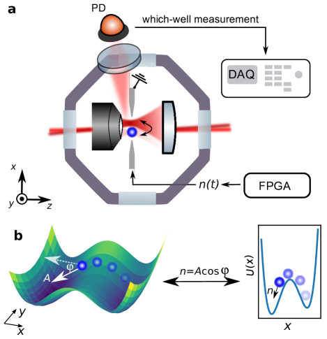
Figure 1: Model under study and experimental setup. a, Experimental setup. We create a bistable optical potential for a charged silica nanoparticle by focusing two cross-polarized beams through a 0.80 NA objective. We implement a which-well measurement by collecting the laterally scattered light with a photodiode (PD). Owing to the different polarizations in the two wells, the intensity measured by the photodiode is a binary signal that indicates in which potential well the particle resides. The particle carries a finite net electric charge and is made active along $x$ with an electrostatic force generated by a voltage applied across lateral electrodes. This voltage is generated by a field-programmable gate array (FPGA). b, A two-dimensional active particle in a potential landscape that is bistable along the $x$-direction and harmonic along $y$. The active particle is propelled by a force of constant magnitude $A$ and Brownian orientation $\varphi$. The dimensions $x$ and $y$ are decoupled and the $x$ motion is equivalent to a particle moving in a one-dimensional bistable potential under a time-dependent force $n(t)=A\cos\varphi(t)$.

I Experimental System

The experimental setup is shown in Fig. 1a. A charged silica nanoparticle of nominal diameter $136\text{\,}\mathrm{n}\mathrm{m}$ is trapped in a bistable optical potential. The bistable potential is realized by focusing two cross-polarized and frequency-shifted Gaussian beams through a high NA objective (wavelength $\lambda=$1064\text{\,}\mathrm{n}\mathrm{m}$$). The two foci lie along the $x$-axis and their distance is controlled by a careful alignment of the relative angle between the beams. To implement a direct which-well measurement, we introduce a photodetector to monitor the light scattered by the particle in a direction perpendicular to the optical axis. Owing to the mutually orthogonal polarization of the two beams, together with the radiation pattern of a linear dipole (which emits no radiation along its axis), the recorded signal displays jumps as the particle transitions from one well to the other. The traces recorded by the photodetector are used for the study of the transition rates presented throughout this work.

We apply an external electrostatic force that mimics the behaviour of active propulsion parallel to the potential’s bistability direction. The voltage signal used to apply the active force is generated by a field-programmable gate array (FPGA), see Methods. Throughout this work, we study a particle actively propelled by a force of constant magnitude $A$, called activity, with stochastically changing direction $\varphi$. After projecting the active force onto the bistability direction $x$, the motion of the particle is described by the following Langevin equations:

$$m\ddot{x}+m\Gamma_{0}\dot{x}+\partial_{x}U(x)=A\cos\varphi+\mathcal{F}_{\text{th}},$$ (1a)

$$\dot{\varphi}=\sqrt{2D_{R}}\eta_{R}(t).$$ (1b)

The position $x$ evolves in time under the influence of a frictional force proportional to the damping coefficient $\Gamma_{0}$, a conservative trapping force arising from the bistable potential $U(x)$, and thermal noise at temperature $T$ related to the friction via the fluctuation-dissipation theorem $\mathcal{F}_{\text{th}}=\sqrt{2m\Gamma_{0}k_{B}T}\eta_{\text{th}}(t)$ Kubo (1966). The two mutually uncorrelated white noises $\eta_{\text{th}}$ and $\eta_{R}$ individually satisfy the properties $\left\langle\eta(t)\right\rangle=0$ and $\left\langle\eta(t)\eta(t^{\prime})\right\rangle=\delta(t-t^{\prime})$. The damping coefficient $\Gamma_{0}$ can be tuned by changing the pressure of the vacuum chamber Beresnev et al. (1990). The orientation of the active force follows overdamped and purely diffusive dynamics associated with the rotational diffusivity $D_{R}$. In the following, we use $n=A\cos{\varphi}$ to refer to the one dimensional active force. The system is illustrated schematically in Fig. 1b.

Figure 2 shows the measured characteristics of the active force, i.e., of the voltage output by our custom-programmed FPGA (see Supplementary Material).

Figure 2: Statistical properties of the active force. The values shown are electric signals which act on the particle through the Coulomb force. a, Transformation of white Gaussian noise through an FPGA into the active force $n=A\cos\varphi$ of equation (1) ($D_{R}=2\pi\times$116\text{\,}\mathrm{k}\mathrm{H}\mathrm{z}$$). b, Probability density of the realized active force in a. The arcsine distribution (dashed line) is expected from the projection onto one dimension of a constant force with fluctuating direction. c, Example spectra of active forces for three different values of $D_{R}$. Panels b and c highlight the non-Markovian and non-Gaussian nature of active propulsion. We refer to the Supplementary Information for a derivation of the theoretical curves shown as dashed lines.

Specifically, in Fig. 2a we show an example time trace of the active force for $D_{R}=2\pi\times$116\text{\,}\mathrm{k}\mathrm{H}\mathrm{z}$$. Figure 2b depicts the histogram of the trace in Fig. 2a, and 2c shows three examples of the power spectral density (PSD) $S_{nn}$ for different rotational diffusivities. In stark contrast to the thermal fluctuations induced by the surrounding gas, the activity’s noise history is non-Gaussian and coloured.

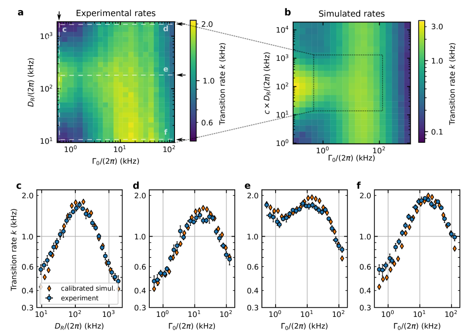
Figure 3: Experimental and numerical transition rates. a, Experimental transition rate constant $k$ as a function of rotational diffusivity $D_{R}$ and translational damping $\Gamma_{0}$. The dashed lines parallel to the arrows refer to the four cuts shown in c, d, e, f. At low $\Gamma_{0}$ we observe the novel active turnover along the $D_{R}$ axis. For fixed $D_{R}$ we recover a Kramers-like turnover. b, Computationally obtained transition rate constant (activity $A=$9.35\text{\,}\mathrm{f}\mathrm{N}$$). The simulated $D_{R}$-axis is rescaled by the calibration factor $c=2.24$, as described in the main text. The transition rate constant agrees within roughly $10\%$ with the calibrated numerical estimates. c, Active turnover. Vertical cut at $\Gamma_{0}=2\pi\times$523\text{\,}\mathrm{H}\mathrm{z}$$ of the experimental (blue circles) and of the simulated (orange diamonds) transition landscapes. d, Horizontal cut at $D_{R}=2\pi\times$1.8\text{\,}\mathrm{M}\mathrm{H}\mathrm{z}$$. High rotational diffusivity in conjunction with sufficiently high friction leads to a recovery of inactive dynamics and of the Kramers turnover. e, Horizontal cut at $D_{R}=2\pi\times$166\text{\,}\mathrm{k}\mathrm{H}\mathrm{z}$$, roughly the position of the active turnover. Starting at high $\Gamma_{0}$ and moving towards lower values, we initially encounter the Kramers-like turnover mainly arising from thermal transitions. Passing the local minimum, a further steady increase in transition rate constant is induced by the active propulsion facilitated by a weaker damping. f, Horizontal cut at $D_{R}=2\pi\times$9\text{\,}\mathrm{k}\mathrm{H}\mathrm{z}$$. As $D_{R}$ approaches zero the active force becomes a modification to the potential with an effectively constant $\varphi$. The resulting Kramers-like turnover results from an average over the corresponding rate constants. Rate extraction and error bars are described in the Methods.

II Results

The central quantity of interest in the present study is the transition rate constant $k$, i.e., the typical frequency of transitions between the metastable states of the potential. It is extracted from the decaying autocorrelation of the which-well measurement (see Methods). Figure 3a showcases the transition rate constant as a function of rotational diffusivity $D_{R}$ and translational damping $\Gamma_{0}$. Each data point stems from a $30\text{\,}\mathrm{s}$ long trajectory with fixed pressure and rotational diffusivity. We observe two perpendicular lines of cross-section maxima. The vertical line of maxima appears at roughly $\Gamma_{0}=2\pi\times$20\text{\,}\mathrm{k}\mathrm{H}\mathrm{z}$$ and corresponds to the Kramers turnover Rondin et al. (2017). The second, horizontal one emerges at $D_{R}=2\pi\times$166\text{\,}\mathrm{k}\mathrm{H}\mathrm{z}$$ and represents the central result of this work: an activity-induced turnover. We additionally depict four cross-sections highlighting the active turnover at $\Gamma_{0}=2\pi\times$523\text{\,}\mathrm{H}\mathrm{z}$$ (Fig. 3c), its passive Kramers counterpart at $D_{R}=2\pi\times$1.8\text{\,}\mathrm{M}\mathrm{H}\mathrm{z}$$ (Fig. 3d), a cut along the rotational diffusivity $D_{R}=2\pi\times$166\text{\,}\mathrm{k}\mathrm{H}\mathrm{z}$$ that corresponds to the active turnover (Fig. 3e), and the Kramers-like turnover at $D_{R}=2\pi\times$9\text{\,}\mathrm{k}\mathrm{H}\mathrm{z}$$ (Fig. 3f). The prominence of the active turnover decreases with increasing damping $\Gamma_{0}$, blends into the Kramers turnover and vanishes for very high dampings.

In order to shed light on the nature of the active turnover, we implemented a numerical reconstruction of the observed transition rate landscape. The numerical reconstruction, displayed in Fig. 3b, aims at recovering the landscape’s key features using three fit parameters: barrier height, activity, and distance between potential wells. The numerical reconstruction is in quantitative agreement with the experimental data throughout the observed parameter space. In addition to the three fit parameters, we introduce a calibration factor $c$ for the rotational diffusivity, needed to bridge the one-dimensional simulation and the more complicated three-dimensional reality: Generally, in higher-dimensional systems it is possible for the particle to prefer different transition channels when driven by the activity or by thermal fluctuations. Such a multiplicity cannot occur in the one-dimensional model of equation (1), it can however easily appear in the experiment, caused for instance by a slight misalignment between potential minima and activity axes. Additional details about the numerical reconstruction can be found in the Methods and Supplementary Material.

III Discussion

The structure of the observed rate landscape in Fig. 3 is surprisingly rich. Nonetheless, its individual features can be understood on the basis of a few intuitive arguments stemming from a more rigorous analysis presented in the Supplementary Material. The existence of a maximum along the $\Gamma_{0}$-axis is analogous to the Kramers turnover in passive systems. Its renewed emergence supports the continued validity of Kramer’s predictions even in non-conservative setups, extending their range of applicability. Next, we focus on the novel aspects arising specifically due to the presence of active propulsion. With the angle evolving according to Brownian motion, equation (1), active propulsion can be interpreted as a stochastic force characterized by an exponentially decaying autocorrelation $\left\langle\cos\varphi(t)\cos\varphi(t^{\prime})\right\rangle=\exp(-D_{R}|t-t^{\prime}|)/2$. This relation identifies the rotational diffusivity as a measure of the characteristic timescale during which the active force’s orientation does not change appreciably: the persistence time $\tau_{A}=D_{R}^{-1}$. This property is the key to reveal the mechanisms underlying the active turnover. To this end, let us conduct a simple thought experiment.

We start from the case of low rotational diffusivity: if the particle’s orientation persists for a very long time, it is possible to consider the barrier to be modified by an additional tilt to the potential of $-Ax\cos\varphi$ (with constant $\varphi$). This modification to the barrier height facilitates the transition in one direction while hampering the reverse one. This trend becomes more apparent as $A$ increases, and at some point we would almost necessarily have to wait for the active force to change its sign to observe the next transition. For very large $A$ and small $D_{R}$ we expect to observe a single transition at best and remain stuck in the temporarily (or practically eternally) favoured well. The rate constant would need to effectively vanish in this extreme scenario.

Very high values of $D_{R}$ affect the system in a fundamentally different manner: if the activity’s direction becomes completely decorrelated on the timescale of small positional displacements, its presence only increases the translational diffusivity in magnitude. In other words, fast rotating active forces raise the particle’s effective temperature. Over the course of a barrier transition the orientation $\varphi$ assumes all its possible realizations and can no longer persistently push the particle over the barrier. The transition rate constant is nevertheless enhanced given that larger diffusivities allow to scale barriers more easily in general. Specifically, as $D_{R}$ is decreased from infinity this effect becomes gradually stronger since the random mean square displacements caused by the activity increase in size on average. This implies a higher effective temperature at lower $D_{R}$ and subsequently higher transition rate constants $k$. The extreme scenario of infinitely fast rotation, on the other hand, will result in no net change of the effective translational diffusion and a recovery of inactive dynamics. Finally, it is reasonable to expect a maximum in the transition rate constant if the persistence time is similar to the characteristic duration necessary to transverse the barrier, namely the average transition path time. Then one typically retains the active force’s aid during the whole transition, without inhibiting the reverse reaction any longer than necessary. Incidentally, this line of thinking closely follows Kramers’ original argument for the existence of the passive turnover as a consequence of two opposing monotonic trends. Here, the position of the maximum is closely tied to the average transition path time as well, roughly emerging when the energy dissipated during the transition is comparable to the thermal energy $k_{\text{B}}T$. The particle’s trajectory then experiences thermal decorrelation that is sufficiently fast to avoid subsequent recrossings (which do not contribute to the rate) without losing the benefit of a more persistent direction of the velocity.

With the timescales of energy dissipation and orientation decorrelation determined by separate parameters, the location of the passive and active turnover on their respective axis become practically independent from changes in the remaining variable, i.e., $D_{R}$ or $\Gamma_{0}$, respectively. This results in the cross-section maxima of Fig. 3 forming two approximately perpendicular lines. The last novel prominent feature, the turnover’s gradual disappearance at large $\Gamma_{0}$, constitutes the property easiest to explain. Any sufficiently high friction can serve to slow down and practically arrest the particle’s movement, leading to the rate constant’s general decrease as one steps farther into the overdamped regime. Conversely, raising $A$ allows the active noise to compete against strong dissipative forces, making the phenomenon relevant for overdamped dynamics as well.

IV Conclusion

We have extended the analysis of the kinetics of transitions in a bistable system to active particles covering both the regimes of overdamped and underdamped motion. We have observed for the first time a novel turnover that arises as the persistence time of the active particle gradually increases from values much shorter to values much longer than the dynamical timescales of the system. A simplified one-dimensional description is sufficient to replicate the rich phenomenology of our experimental findings, and is capable of generating quantitatively consistent predictions. A full closed-form description that bridges the low with the high rotational diffusivity limits remains an open question tied to the complexity of the underlying Fokker-Planck equation.

Our experimental platform can be adapted in the future to address various theoretical concepts arising in stochastic thermodynamics involving non-equilibrium systems and correlated noise histories. For instance, with the inclusion of a linear position measurement across a wide region of space, we can extend the model to a full three-dimensional activity rather than a one-dimensional projection. This setup would enable a rigorous investigation on the statistics of transition path times and the emergence of different pathways preferred by active and thermal transitions as a function of the activity. With the inclusion of a position feedback we can generate more complex kinds of position- and time-dependent activities, which have recently been shown to have intriguing tactic properties Geiseler et al. (2017). Furthermore, our externally applied stochastic force is not inherently constrained to mimic active propulsion, but rather allows for the introduction of any desired noise history into the system. This versatility opens up experimental opportunities in the field not tied to activity, such as fluctuation theorems in the presence of coloured noise.

V Methods

Experimental setup. The frequency shift ($80\text{\,}\mathrm{M}\mathrm{H}\mathrm{z}$) between the two beams is introduced by an acousto-optic modulator (AOM) acting on a $\lambda=$1064\text{\,}\mathrm{n}\mathrm{m}$$ wavelength laser. The AOM also controls the power of the two beams, equal to $70\pm 1$ ($110\pm 1$) mW for the $x$- ($y$-) polarized beam. After the focus, the beams are recollimated and separated with a polarizing beam splitter (PBS). We use a standard homodyne position measurement on the $x$-polarized beam to characterize the potential curvatures Gieseler et al. (2012). The curvatures are estimated through time-frequency analysis: the estimated values are $\omega_{1}=2\pi\times(73.0\pm 0.5)$ kHz for the $x$-polarized well and $\omega_{2}=2\pi\times(82\pm 4)$ kHz for the $y$-polarized well. The proportionality coefficient between damping and pressure is inferred via the power spectral density (PSD) of the particle when the $y$-polarized laser is turned off Hebestreit et al. (2018). Specifically, the PSD of a harmonic oscillator is given by a Lorentzian whose width equals the damping coefficient.

Active force. The active force is realized with a field-programmable gate array (FPGA) that takes as input a white noise created by a function generator. The FPGA integrates equation (1b) to generate the active force as output. We exploit the net charge carried by the particle and apply the active force electrostatically through two electrodes mounted along the bistability direction Frimmer et al. (2017). The experimental value of the activity can be determined from the response of the particle to a known modulated voltage. Within 50% accuracy due to the mass uncertainty, we estimated $A=$6.8\text{\,}\mathrm{f}\mathrm{N}$$. A potential barrier height $\Delta U$ of a few $k_{\text{B}}T$ and diffraction limited width $\Delta x\approx\lambda/2$ gives rise to conservative forces with a typical magnitude of $\Delta U/\Delta x\approx$8\text{\,}\mathrm{f}\mathrm{N}$$. In order to induce a measurable effect the activity needs to be of the same order of magnitude, as is the case here.

Transition rate estimation. Rate coefficients appear within the framework of the eponymous rate equations. This type of differential equation aims to describe the evolution of local concentrations or population fractions in a set of states $\{A,B,\dots\}$ subjected to reactive transitions. Our case, a bistable system with population fractions $c_{A}$ and $c_{B}$, represents a particularly simple example described by $\dot{c}_{A}=-k_{AB}c_{A}+k_{BA}c_{B}=k(c_{A,eq}-c_{A})$. With the asymmetry between rate constants $k_{AB}$ and $k_{BA}$ attributable to the stationary concentration $c_{A,eq}=k_{BA}/(k_{AB}+k_{BA})$, the transition rate $k$ represents the dynamical parameter governing the speed of equilibration. Within the approximation of rate equations, $c_{A}(t)=(c_{A}(0)-c_{A,eq})e^{-kt}+c_{A,eq}$ approaches its equilibrium value exponentially and the rate can be extracted from sufficiently long sample trajectories Rondin et al. (2017). The rates in Fig. 3, more specifically, are extracted from $30\text{\,}\mathrm{s}$ long trajectories. We split each trajectory in ten segments and compute the average rate and its standard deviation.

Numerical reconstruction. The simulation results complementing our experimental findings stem from the optimization of an effective, one-dimensional potential along with the activity A. We use a bistable, piece-wise parabolic potential, continuous up to its first derivative and tune its barrier width/curvature $\omega_{B}$ and height $h$. Equation (1) is then numerically integrated for values of $\Gamma_{0}$ and $D_{R}$ spaced on a logarithmic grid. We employ the OVRVO integrator devised by Sivak et al. for the particle’s propagation Sivak et al. (2014). The curvatures of the well-parabolas respect the experimentally determined particle frequencies. The obtained transition landscapes are compared to the experimental reference w.r.t. a small number of effective quantities related to the active and passive turnover, respectively: maximum height, its position on the respective axis, and turnover width at half maximum, all evaluated on a logarithmic scale. We proceed to locate the parameter set of $h$, $\omega_{B}$, and $A$ that leads to the minimal deviation in the aforementioned measures on a discrete, linearly spaced grid of desired resolution. Starting from cautious a-priori estimates of these values, we rely on a bisection-like approach to locate said minimum. To simplify this procedure, note that at high $D_{R}$ one essentially recovers inactive dynamics, allowing us to optimize $h$ and $\omega_{B}$ independently of $A$. Additional details on the simulation and optimization procedure can be found in the Supplementary Material.

VI Acknowledgements

This research was supported by the Swiss National Science Foundation (grant no. 200021L_169319 and no. 51NF40-160591) and the Austrian Science Fund (grant no. I3163-N36). The authors acknowledge P. Back, E. Bonvin, F. van der Laan, A. Nardi, J. Piotrowski, R. Reimann and D. Windey for fruitful discussions.

References

- Arrhenius (1889) S. Arrhenius, Z. Phys. Chem. 4U, 226 (1889).
- van’t Hoff (1884) J. H. van’t Hoff, Recl. Trav. Chim. Pays-Bas 3, 333 (1884).
- Ricci et al. (2017) F. Ricci, R. A. Rica, M. Spasenovic, J. Gieseler, L. Rondin, L. Novotny, and R. Quidant, Nat. Commun. 8, 1 (2017).
- Landauer and Swanson (1961) R. Landauer and J. A. Swanson, Phys. Rev. 121, 1668 (1961).
- Šali et al. (1994) A. Šali, E. Shakhnovich, and M. Karplus, Nature 369, 248 (1994).
- Frauenfelder et al. (1991) H. Frauenfelder, S. G. Sligar, and P. G. Wolynes, Science 254, 1598 (1991).
- Beece et al. (1980) D. Beece, L. Eisenstein, H. Frauenfelder, D. Good, M. C. Marden, L. Reinisch, K. T. Yue, A. H. Reynolds, and L. B. Sorensen, Biochemistry 19, 5147 (1980).
- D’Agliano et al. (1975) E. G. D’Agliano, P. Kumar, W. Schaich, and H. Suhl, Phys. Rev. B 11, 2122 (1975).
- Bohr and Wheeler (1939) N. Bohr and J. A. Wheeler, Phys. Rev. 56, 426 (1939).
- Silvestrini et al. (1988) P. Silvestrini, S. Pagano, R. Cristiano, O. Liengme, and K. E. Gray, Phys. Rev. Lett. 60, 844 (1988).
- Eyring (1935) H. Eyring, J. Chem. Phys. 3, 63 (1935).
- Hänggi et al. (1990) P. Hänggi, P. Talkner, and M. Borkovec, Rev. Mod. Phys. 62, 251 (1990).
- Kramers (1940) H. A. Kramers, Physica 7, 284 (1940).
- Grabert and Linkwitz (1988) H. Grabert and S. Linkwitz, Phys. Rev. A 37, 963 (1988).
- McCann et al. (1999) L. I. McCann, M. Dykman, and B. Golding, Nature 402, 785 (1999).
- Turlot et al. (1989) E. Turlot, D. Esteve, C. Urbina, J. M. Martinis, M. H. Devoret, S. Linkwitz, and H. Grabert, Phys. Rev. Lett. 62, 1788 (1989).
- Troe (1986) J. Troe, in J. Phys. Chem., Vol. 90 (1986) pp. 357–365.
- Rondin et al. (2017) L. Rondin, J. Gieseler, F. Ricci, R. Quidant, C. Dellago, and L. Novotny, Nat. Nanotechnol. 12, 1130 (2017).
- Hanggi and Mojtabai (1982) P. Hanggi and F. Mojtabai, Phys. Rev. A 26, 1168 (1982).
- Pollak (1986) E. Pollak, J. Chem. Phys. 85, 865 (1986).
- Pollak et al. (1989) E. Pollak, H. Grabert, and P. Hänggi, J. Chem. Phys. 91, 4073 (1989).
- Pollak and Ankerhold (2013) E. Pollak and J. Ankerhold, J. Chem. Phys. 138, 164116 (2013).
- Bechinger et al. (2016) C. Bechinger, R. Di Leonardo, H. Löwen, C. Reichhardt, G. Volpe, and G. Volpe, Rev. Mod. Phys. 88, 045006 (2016).
- Volpe et al. (2014) G. Volpe, S. Gigan, and G. Volpe, Am. J. Phys. 82, 659 (2014).
- Howse et al. (2007) J. R. Howse, R. A. Jones, A. J. Ryan, T. Gough, R. Vafabakhsh, and R. Golestanian, Phys. Rev. Lett. 99, 048102 (2007).
- Romanczuk et al. (2012) P. Romanczuk, M. Bär, W. Ebeling, B. Lindner, and L. Schimansky-Geier, Eur. Phys. J. Special Topics 202, 1 (2012).
- Ghosh et al. (2013) P. K. Ghosh, V. R. Misko, F. Marchesoni, and F. Nori, Phys. Rev. Lett. 110, 268301 (2013).
- Golestanian et al. (2007) R. Golestanian, T. B. Liverpool, and A. Ajdari, New J. Phys. 9, 126 (2007).
- Sundararajan et al. (2008) S. Sundararajan, P. E. Lammert, A. W. Zudans, V. H. Crespi, and A. Sen, Nano Lett. 8, 1271 (2008).
- Berg (2004) H. C. Berg, E. coli Motion, edited by H. C. Berg, Biological and Medical Physics, Biomedical Engineering (Springer New York, New York, NY, 2004).
- Gejji et al. (2012) R. Gejji, P. M. Lushnikov, and M. Alber, Phys. Rev. E 85, 021903 (2012).
- Brenner (1990) H. Brenner, Langmuir 6, 1715 (1990).
- Bressloff and Newby (2013) P. C. Bressloff and J. M. Newby, Rev. Mod. Phys. 85, 135 (2013).
- Ebbens and Howse (2010) S. J. Ebbens and J. R. Howse, Soft Matter 6, 726 (2010).
- Geiseler et al. (2016) A. Geiseler, P. Hänggi, and G. Schmid, Eur. Phys. J. B 89, 175 (2016).
- Schaar et al. (2015) K. Schaar, A. Zöttl, and H. Stark, Phys. Rev. Lett. 115, 038101 (2015).
- Pohlmann and Tributsch (1997) L. Pohlmann and H. Tributsch, Electrochim. Acta 42, 2737 (1997).
- Burada and Lindner (2012) P. S. Burada and B. Lindner, Phys. Rev. E 85, 032102 (2012).
- Scholz et al. (2018) C. Scholz, S. Jahanshahi, A. Ldov, and H. Löwen, Nat. Commun. 9, 1 (2018).
- Kubo (1966) R. Kubo, Reports Prog. Phys. 29, 255 (1966).
- Beresnev et al. (1990) S. A. Beresnev, V. G. Chernyak, and G. A. Fomyagin, J. Fluid Mech. 219, 405 (1990).
- Geiseler et al. (2017) A. Geiseler, P. Hänggi, and F. Marchesoni, Sci. Rep. 7, 1 (2017).
- Gieseler et al. (2012) J. Gieseler, B. Deutsch, R. Quidant, and L. Novotny, Phys. Rev. Lett. 109, 103603 (2012).
- Hebestreit et al. (2018) E. Hebestreit, M. Frimmer, R. Reimann, C. Dellago, F. Ricci, and L. Novotny, Rev. Sci. Instrum. 89, 033111 (2018).
- Frimmer et al. (2017) M. Frimmer, K. Luszcz, S. Ferreiro, V. Jain, E. Hebestreit, and L. Novotny, Phys. Rev. A 95, 061801 (2017).
- Sivak et al. (2014) D. A. Sivak, J. D. Chodera, and G. E. Crooks, J. Phys. Chem. B 118, 6466 (2014).