Quantum Technology for Economists111The opinions expressed in this article are the sole responsibility of the authors and should not be interpreted as reflecting the views of Sveriges Riksbank.
Abstract
Research on quantum technology spans multiple disciplines: physics, computer science, engineering, and mathematics. The objective of this manuscript is to provide an accessible introduction to this emerging field for economists that is centered around quantum computing and quantum money. We proceed in three steps. First, we discuss basic concepts in quantum computing and quantum communication, assuming knowledge of linear algebra and statistics, but not of computer science or physics. This covers fundamental topics, such as qubits, superposition, entanglement, quantum circuits, oracles, and the no-cloning theorem. Second, we provide an overview of quantum money, an early invention of the quantum communication literature that has recently been partially implemented in an experimental setting. One form of quantum money offers the privacy and anonymity of physical cash, the option to transact without the involvement of a third party, and the efficiency and convenience of a debit card payment. Such features cannot be achieved in combination with any other form of money. Finally, we review all existing quantum speedups that have been identified for algorithms used to solve and estimate economic models. This includes function approximation, linear systems analysis, Monte Carlo simulation, matrix inversion, principal component analysis, linear regression, interpolation, numerical differentiation, and true random number generation. We also discuss the difficulty of achieving quantum speedups and comment on common misconceptions about what is achievable with quantum computing.
Keywords: Quantum Computing, Econometrics, Computational Economics, Money, Central Banks.
JEL Classification: C50, C60, E40, E50.
1 Introduction
The field of quantum technology is divided into four broad areas: quantum computing, quantum simulation, quantum communication, and quantum sensing. Quantum computing centers around the exploitation of quantum physical phenomena, such as superposition and entanglement, to perform computation. Quantum simulation involves the development and use of specialized devices to simulate a specific quantum physical processes. Quantum communication studies how quantum phenomena can be used to securely transmit information between parties. And quantum sensing and metrology make use of quantum phenomena to produce more accurate sensors and measurement devices than could be created using existing classical technologies.
Research on quantum technology has largely been confined to a discussion between computer scientists, physicists, engineers, and mathematicians. Our objective in this manuscript is to widen the conversation to include economists, focusing on two areas in which quantum technology is likely to have relevance for the discipline: (1) the use of quantum computing to solve and estimate economic models; and (2) the use of quantum communication to construct forms of currency called “quantum money,” which have novel properties that cannot be achieved without exploiting quantum phenomena.333Those who have a broader interest in quantum technology may want to see Johnson et al. (2014) for an overview of quantum simulation; Gisin and Thew (2007) for an overview of quantum communication; and Giovannetti et al. (2011) and Degen et al. (2017) for an overview of quantum sensing and metrology.
Our examination of quantum computing will focus primarily on quantum algorithms, but will also provide a brief overview of the experimental efforts to develop quantum computing devices. Similarly, our discussion of quantum money will center on theoretical constructions, but will also review experimental progress in its implementation. Throughout the manuscript, we will assume that the reader has no knowledge of physics, but is familiar with probability theory and linear algebra. Furthermore, we will provide a sufficient amount of low-level detail to enable economists to identify points of entry into the existing literature and to contribute with novel research. An econometrician, for instance, will be able to identify what problems remain in the construction of quantum versions of familiar classical algorithms, such as ordinary least squares (OLS) and principal component analysis (PCA).
We will start our exploration of quantum computing and quantum money with an overview of preliminary material, limiting ourselves to a narrow selection of topics that will provide a foundation for understanding basic algorithms and money schemes. This material covers a mathematical and notational description of quantum computers and their functions, including descriptions of the creation and manipulation of quantum states. It also covers theory relevant to the construction of quantum money schemes. Part of the purpose of this section is to communicate how quantum physical phenomena, such as superposition, entanglement, and the no-cloning theorem provide new computational and cryptographic resources.
We will also see how quantum states can be manipulated using quantum operations to perform computation. This includes a description of what types of operations are permissible and how this translates into mathematics. Once the operations have been executed and the computation is complete, we must offload the results to a classical computer. Since the results take the form of a quantum state, we will need to perform measurement, a process that yields a classical state and is analogous to sampling. Understanding measurement will clarify why quantum computers are not simply classical computers with a special capacity for parallel computation: we can only output as much classical information as we input.
In addition to providing a mathematical and notational description of quantum computation, we will also discuss the practicalities of implementing computations in the form of quantum circuits. Such circuits can be simulated classically or run on a quantum computer. We will also introduce the notion of oracles from computer science, which we will use in some cases to determine the size of a quantum speedup; and the no-cloning theorem (Wootters and Zurek, 1982), which will be essential for the construction of quantum money schemes.
After covering the preliminary material, we will discuss two topics of interest for economists: quantum money and quantum algorithms. The original motivation for quantum money, as given in Wiesner (1983), was to construct a form of currency that was “physically impossible to counterfeit.” This differs categorically from existing forms of money, which do not exploit quantum phenomena and are therefore vulnerable to attack from counterfeiters. In addition to reverse-engineering threads and inks, and breaking encryption schemes, an attacker could, in principle, copy any “classical” form of money bit-by-bit or even atom-by-atom, as no physical law prohibits it.444Here, we use the term “classical” to indicate that the money or payment instrument does not make use of quantum physical phenomena.
Indeed, such attacks are not merely of theoretical interest. Counterfeiting necessitates costly periodic note and coin re-designs, and forces the general public to do currency checking (Quercioli and Smith, 2015). State actors have also used counterfeiting to circumvent international sanctions and conduct economic warfare.555Large-scale counterfeiting has been attempted as a means of undermining public confidence in the monetary system. During World War II, for instance, a Nazi plot called “Operation Bernhard” exploited Jewish prisoners in an attempt to counterfeit large quantities of British pounds, with the intention to circulate them via an airdrop (Pirie, 1962). The Bank of England responded by withdrawing notes above £5 from circulation. See: https://www.bankofengland.co.uk/museum/online-collections/banknotes/counterfeit-and-imitation-notes. There are also historic records of mass counterfeiting attempts by England during the French revolution (Dillaye, 1877, p. 33). Prior to the development of fiat currencies, gold and other forms of commodity money relied on intrinsic worth, natural scarcity, and widespread cognizability to safeguard their value against attacks. Even with these natural advantages, high-quality counterfeits were still produced and passed to uninformed merchants.666Certain forms of commodity money can also be synthesized from other materials. Gold, for instance, can be synthesized, but not yet cost-effectively (Aleklett et al., 1981). Even if a form of commodity money’s value is safeguarded against large-scale synthesization, the discovery of new deposits or improvements in extraction technology constitute supply shocks that could lead to substantial devaluations. In contrast to existing forms of currency, quantum money is protected by the no-cloning theorem, which makes it impossible to counterfeit by the laws of physics. Along with post-quantum cryptography and quantum key distribution, it also provides a means of protecting the payments system against future quantum attacks.777Shor (1994) introduced a near-exponential quantum speedup to prime factorization, which compromises the commonly-used RSA encryption algorithm. Cryptocurrencies, such as Bitcoin, are also subject to attack from quantum computers (Aggarwal et al., 2018).
Our overview of quantum money starts with a full description of the original scheme, which was introduced circa 1969, but only published later in Wiesner (1983). We will see that it achieves what is called “information-theoretic security,” which means that an attacker with unbounded classical and quantum resources will not be able to counterfeit a unit of the money.888Technically, such an adversary might successfully counterfeit the money, but this happens with exponentially small probability in the size of the quantum system. Therefore, by constructing a large enough quantum system, the success probability could easily be made , which is effectively for all practical concerns. Since this original scheme was proposed, the term “quantum money” has come to refer to a broad variety of different payment instruments, including credit cards, bills, and coins, all of which use of quantum physical phenomena to achieve security.
The real promise of quantum money is that it offers the possibility of combining the beneficial features of both physical cash and digital payments, which is not possible without the use of the higher standard of security quantum money offers. In particular, a form of currency called “public-key” quantum money would allow individuals to verify the authenticity of bills and coins publicly and without the need to communicate with a trusted third party. This is not possible with any classical form of digital of money, including cryptocurrencies, which at least require communication with a distributed ledger. Thus, quantum money could restore the privacy and anonymity associated with physical money transactions, while maintaining the convenience of digital payment instruments.
While quantum money offers features that are unachievable in any classical form of currency, implementing a full quantum money scheme requires additional advances in quantum technology. However, recent progress in the development of quantum money has moved us closer to a full implementation. Partial schemes have already been experimentally implemented for variants of private-key quantum money (Bozzio et al., 2018; Guan et al., 2018; Bartkiewicz et al., 2017; Behera et al., 2017). In all cases, quantum memory remains the primary bottleneck to a full implementation, as existing technologies are not able to retain a quantum state for longer than a fraction of a second. Furthermore, the challenges to implementation are even more substantial for public-key money schemes, which have not yet been partially implemented in an experimental setting. Public-key quantum money also faces formidable theoretical challenges, which may be of particular interest to those working on mechanism design.
In addition to quantum money, we also examine quantum algorithms, which offer the possibility of achieving speedups over their classical counterparts. Since quantum computing makes use of different computational resources than classical computing, we must create entirely new algorithms to achieve such speedups; and cannot simply rely on the parallelization of classical algorithms, as we have, for instance, with GPU (graphics processing unit) computing. This suggests that it will be necessary to develop literatures on quantum econometrics and quantum computational economics. Fortunately, outside of economics, the literature on quantum algorithms has already produced quantum versions of several econometric and computational-economic routines. These routines, however, typically have limitations that do not apply to their classical counterparts. We will both discuss those limitations and also indicate where economists may be able to contribute to the literature.
Our objective in the quantum algorithms section will be to provide a complete review of relevant algorithms for economists, including function approximation, linear systems analysis, Monte Carlo simulation, matrix inversion, principal component analysis, linear regression, interpolation, numerical differentiation, and true random number generation. In some cases, quantum algorithms will achieve an exponential speedup over their classical counterparts, rendering otherwise intractable problems into something that may eventually be feasible to perform on a quantum computer. In other cases, quantum algorithms will alleviate memory constraints that may render certain problems intractable on classical computers by allowing them to be performed with exponentially fewer input resources. In each case, we will describe the original or most commonly-used version of the algorithm in low-level detail, along with its limitations, and then provide an up-to-date description of related work in the literature.
We also go beyond a description of individual quantum algorithms to discuss the underlying mechanism for generating speedups in many quantum algorithms, which is non-trivial. This involves a discussion of phase kickback, phase estimation, and the quantum Fourier transform, which are three common ingredients in many quantum algorithms that achieve a speedup over their classical counterparts. Economists who wish to develop future literatures on quantum econometrics or quantum computational economics will need to understand these concepts.
In addition to reviewing quantum algorithms that have relevance for economists, we also provide an overview of experimental progress in the development of quantum computers. Benchmarking quantum advantage typically involves computational problems that require large amounts of memory and logical operations on classical high-performance computers (HPC). As such, a quantum algorithm may need to run anywhere from minutes to days to demonstrate a speedup over its classical equivalent. At present, quantum algorithms must be executed on noisy intermediate scale quantum (NISQ) devices (Preskill, 2018) with up to 54 qubits (Arute et al., 2019) and a few hundred gates. While such devices are on the threshold of exceeding the memory capacity of present and future HPCs, demonstrating a quantum advantage will also typically require the execution of a large sequence of operations. This, in turn, will require considerably longer coherence times in quantum circuits or efficient quantum error correction (QEC). Consequently, in the near-term, applications of quantum computing will be limited to proof-of-principle demonstrations and to the development of quantum awareness and education. Moreover, the challenge of achieving quantum speedups is likely to contribute to the development of more efficient classical algorithms.
The remainder of the paper is organized as follows. Section 2 provides an overview of preliminary material that is needed to fully understand quantum money and quantum algorithms. This includes mathematical and notational descriptions of quantum physical phenomena, as it is used to perform computation. Section 3 introduces the concept of quantum money, including the complete technical details for the first quantum money scheme and an overview of all of the major theoretical and experimental contributions to the literature. Section 4 provides an exhaustive literature review of quantum algorithms that can be employed to solve and estimate economic models, along with descriptions of how such algorithms can be implemented and whether they face limitations relative to their classical counterparts. It also describes the current status of quantum hardware and software. Finally, Section 5 concludes, and the Appendix provides additional technical detail on quantum money and quantum algorithms.
2 Preliminaries
This section will provide an overview of concepts from quantum computing and quantum money that assume knowledge of linear algebra and statistics, but not of physics or computer science. The set of topics covered is intended to be as narrow as is possible while still providing readers with a basis for understanding simple quantum algorithms and quantum money schemes. We will discuss how information is encoded in physical systems, how the states of such systems are represented mathematically, and what operations can be performed on them. For a more complete overview of quantum computing, see the section on “Fundamental Concepts” in Nielsen and Chuang (2000), the section on “Quantum Building Blocks” in Polak and Rieffel (2011), or the lecture notes for John Watrous’s introductory course on Quantum Computing (Watrous, 2006).
2.1 Quantum States
In this subsection, we will discuss quantum states, which are the media in which information in quantum computers is stored. States may be acted on by operations to perform computation.
2.1.1 Quantum Bits
A binary digit or “bit” is the fundamental unit of classical computing. Bits can be in either a 0 or 1 position and may be encoded physically using classical systems with two states. In modern computers, it is common to encode the 0 position with a low voltage level and the 1 position with a high voltage level. The choice to use bits allows for the direct application of Boolean logical operations. Table I shows a selection of such operations. As proven by Sheffer (1913), universal computation can be performed using only the NOT-AND (NAND) operation and pairs of bits.999A universal computer is capable of simulating any other computer. Thus, a classical computer that uses complex logical operations with many inputs will not be capable of performing different operations than a computer that exclusively performs NANDs on pairs of bits.
| State | AND | OR | XOR | NAND |
|---|---|---|---|---|
| 00 | 0 | 0 | 0 | 1 |
| 01 | 0 | 1 | 1 | 1 |
| 10 | 0 | 1 | 1 | 1 |
| 11 | 1 | 1 | 0 | 0 |
A quantum bit or “qubit” is the fundamental unit of quantum computing. As with classical bits, quantum bits are encoded in two-level systems; however, unlike classical bits, qubits are encoded in quantum systems, such as photon polarizations, electron spins, and energy levels. The use of quantum systems allows for the exploitation of quantum physical properties. For instance, rather than being restricted to either the 0 or 1 position (like classical bits), quantum bits may be in a superposition of both 0 and 1 simultaneously. We will discuss how such properties – superposition, entanglement, and interference – may be used to provide an advantage over what is achievable using classical bits in Sections 2.1.4 and 2.1.5.
Importantly, quantum computing can be performed without a deep understanding of the physical processes that underlie it, just as it is possible to perform classical computing without an understanding of the underlying physical systems that encode information. While an understanding of quantum physics may improve intuition, it will be sufficient to understand how states are represented and what operations we may perform on them. The purpose of this section will be to provide such information through a primarily mathematical description.
2.1.2 Vector Representation
Individual classical bits are limited to two configurations: 0 and 1. If, for instance, we have five bits – 0, 1, 1, 0, and 0 – we can represent the underlying state of the system using a five-digit bit string: 01100. More generally, if we have bits – 0, 1, …, 1 – we can represent the underlying state with the n-digit bit string: 01…1. This is not true for qubits. In addition to being in the two “classical” states, 0 or 1, a two-level quantum system may also be in an uncountably infinite number of superposition states. For this reason, we represent an individual qubit using a column vector, as shown in Equation (1).
| (1) |
Note that and are referred to as “amplitudes” and lie in . Furthermore, as shown in Equation (2), the modulus squared of each of the elements sums to one.101010If , then we may decompose into real and imaginary parts, , where . The modulus of a complex number is .
| (2) |
If we have a second two-level system, the joint state of the first and second systems is given by their tensor product, as shown in Equation (3).
| (3) |
As we have seen, a single qubit state is in and a two-qubit state is in . More generally, an n-qubit state will lie in . This means that an -qubit quantum system is capable of representing complex numbers; whereas, an -bit classical system is only capable of representing binary digits. This exponential scaling in computational resources that arises from a linear scaling in the number of qubits provides the basis for quantum speedups. Importantly, however, as we discuss in Section 4.2.2, this will not lead to general exponential gains with respect to resource requirements or run times.
2.1.3 Dirac Notation
While it is possible to represent quantum states using column vectors, it will often be more convenient to use bra-ket notation, introduced by Dirac (1939). This is because the size of the column vector needed to represent the state of a system scales exponentially with the number of qubits. A 20-qubit system, for instance, will require a 1,048,576-element column vector.
As you may have noticed in the previous subsection, our column vector representation may be reformulated in terms of basis vectors, as shown in Equation (4). Dirac notation simplifies the more cumbersome column vector representation by using “kets” to represent quantum states.
| (4) |
In Equation (4), we have used what is referred to as the “computational basis,” which is given in Equation (5).
| (5) |
In Dirac notation, we will use the ket, , to represent the underlying state of the system. We can also decompose the state using basis vector kets: . This reformulation is given in Equation (6).
| (6) |
Furthermore, if we have multiple qubits, and , their state will be the tensor product of the two individual qubit states, which may be written in any of the ways shown in Equation (7).
| (7) |
Since tensor products satisfy the distributive property, we may re-express Equation (7) as Equation (8).111111Tensor products satisfy the distributive and associative properties, but not the commutative property.
| (8) |
In addition to the computational basis, it will often be convenient to use other bases, including the Hadamard basis: . Note that and are defined in Equations (9) and (10).
| (9) |
| (10) |
In addition to the ket, Dirac notation also introduces the bra, which is the conjugate transpose of the ket. Equation (11) defines the bra that corresponds to .
| (11) |
Note that and are the complex conjugates of and .121212If , then . The bra will be useful notationally when we wish to express an inner or outer product, which will be used frequently. The inner product of and is expressed in Equation (12).
| (12) |
The equivalent outer product is defined in Equation (13).
| (13) |
2.1.4 Superposition
In the computational basis, a superposition is a linear combination of the two basis states, and : . Pure states in the computational basis, and , are also superpositions in different bases. Note that we may write , which is a pure state in the computational basis, as a superposition in the Hadamard basis, as shown in Equation (14).
| (14) |
The ability to create quantum superpositions will provide us with a computational resource that is not available in classical computing. While a classical bit must be in either the 0 or 1 position, a qubit may be in an uncountably infinite number of linear combinations of the and states.
As we will discuss in Section 2.3, we cannot observe the amplitudes associated with a superposition. Rather, we are restricted to performing measurement on a state in a particular basis, which will cause the superposition to collapse into a basis state. For instance, upon measurement in the computational basis, would yield with probability and with probability .
2.1.5 Entanglement
Most multi-qubit states can be written as tensor products, such as or . However, some states, which are said to be “entangled,” cannot be expressed in such a way. Rather, these states exhibit “correlation” in the sense that measurement of one qubit yields information about the states of the remaining unmeasured qubit(s).
There are four maximally-entangled two-qubit states, which are referred to as the Bell states and were introduced in Bell (1964) as a resolution to the paradox in Einstein et al. (1935). One such Bell state is is defined in Equation (15).
| (15) |
Notice that no choice of amplitudes – , , , and – will satisfy Equation (16).
| (16) |
Importantly, entanglement does not reduce to the concept of correlation in classical probability. Rather, if we measure the first qubit in using the computational basis, we will get either or with probability . If our measurement returns for the first qubit, we will also get for the second with certainty. Alternatively, if we get for the first qubit, we will get for the second qubit.
This property of entangled quantum states remains true even if we separate the qubits in space and perform measurement simultaneously. It is sometimes referred to as non-locality, since the speed of interactions does not appear to depend on physical proximity. Entanglement plays an important role in several quantum algorithms. It also used in the quantum teleportation protocol and features prominently in proposals for secure communication via a quantum internet.
2.2 Quantum Dynamics
The evolution of quantum states over time can be described using unitary operations. The necessary and sufficient condition for the unitarity of a matrix, , is that . Note that is the adjoint operator, defined in Equation (17), which transposes and takes the complex conjugate of each of its elements.
| (17) |
Unitary operations preserve the Euclidean norm, which ensures that quantum states maintain a Euclidean length of 1 post-transformation. Furthermore, unitary operations are trivially invertible through the use of the adjoint operator, allowing for reversibility, which is a requirement of quantum computation.131313This is a consequence of the Schrödinger equation, which describes the time evolution of a quantum system and is reversible. Note that there is no such requirement for classical computing. If, for instance, we apply an AND gate to 0 and 1 input bits in a classical circuit, we get the output 0. Without additional information, we cannot reverse that 0 to recover 0 and 1, since inputs of 0 and 0 would also yield a 0.
The simplest operations are single-qubit unitaries. Among these, commonly-applied unitaries include the identity operator, , and the Pauli operators – , , and – which are defined in Equation (18).
| (18) |
The identity operator leaves the quantum state unchanged. The Pauli X unitary applies a “bit flip” or NOT operation, as shown in Equation (19). That is, becomes , becomes , and, more generally, becomes .
| (19) |
The Pauli Z unitary applies a relative phase flip. That is, it changes the sign of the the second amplitude. In the computational basis, this will shift a state to a state and a state to a state, as shown in Equation (20).
| (20) |
As shown in Equations (21) and (22), the Pauli Y unitary acts as a NOT operation in both the computational and Hadamard bases.
| (21) |
| (22) |
Note that the in Equation (21) and the in Equation (22) are referred to as global phases. Since quantum states are only unique up to a global phase, we may treat as and as .
In addition to the Pauli operators, the Hadamard operator, , is also frequently used in quantum algorithms, including the quantum Fourier transform (QFT).141414See A.4 in the Appendix for an overview of the quantum Fourier transform. When applied to computational basis states, the Hadamard operator creates an equal superposition of the and states, as shown in Equations (23) and (24). The Hadamard operator also transforms states in the Hadamard basis to the computational basis: , and .
| (23) |
| (24) |
Beyond the I, X, Z, Y, and H single-qubit unitaries, many quantum algorithms will require the use of rotation matrices, including the phase operation, , and the operation, , which are defined in Equation (25).
| (25) |
To create entanglement between qubits, we will use the controlled-NOT or CNOT operation. This two-qubit operation has a control qubit and a target qubit. If the control qubit is in the position, then the operation will be applied to the target qubit. In Equation (26), we apply a CNOT, , to the quantum state, .
| (26) |
In addition to the operations, we will use to denote arbitrary controlled-unitary operations, such as , , or . However, in order to perform any quantum computation, , , , , , , , and will be sufficient, since they form a universal set of operations.
More generally, we may perform -qubit operations using the tensor products of each of the single-qubit operations. For instance, applying an operation to qubit 1 and an operation to qubit 2 in the state is equivalent to applying to , as is shown in Equation 27.
| (27) |
Finally, while we have discussed everything in terms of unitary operations thus far, we will also use the term “gates” to refer to the implementation of such operations in quantum circuits. We will introduce quantum circuits and gates in Section 2.4.
2.3 Quantum Measurement
In quantum algorithms, measurement is performed before reading out the results to a classical computer. As shown in Born (1926), this triggers a “collapse of the wavefunction.” For an arbitrary state, such as , this means that the superposition will collapse into a pure state in the basis in which it is measured. If the computational basis is selected, the probability of outcome will be and the probability of outcome will be . These probabilities are computed for using and using . Note that these are not observable, but we can infer them by repeatedly preparing the same state and then performing measurement.
Measurements on multi-qubit states also work the same. Consider, for instance, an equal superposition of two qubits, as shown in Equation (28). The probability of measuring any of the four possible states is given by . Furthermore, upon measurement, the superposition will collapse into , , , or .
| (28) |
It is also possible to perform a partial measurement on just one qubit. If, for instance, we measure just the first qubit, the probability of getting will be . This is because there are two states for qubit two associated with a state for qubit one. The probabilities associated with these states sum to . Furthermore, if we measure qubit one and find it to be in state , then the state of the second, unmeasured qubit will be . We can see this by rewriting as . Note that the amplitude must be renormalized to after measurement, since the probabilities will otherwise not sum to one.
2.4 Quantum Circuits
A quantum circuit is a model of quantum computation that consists of initial states, gates, wires, and measurement. Circuits are typically initialized with as the state for each qubit. Gates, which are unitary operations acting non-trivially only on a constant number of qubits, are then applied in sequence. Finally, a measurement is performed at the end of the circuit, collapsing the superpositions of the measured qubits. Note that circuit diagrams should be read from left to right.
Figure I provides a diagram of a circuit that performs true random number generation from a Bernoulli distribution with parameters . On the left side of the circuit, one qubit is initialized in state . The Hadamard gate, indicated by the H inscribed within a rectangle, is then applied to the qubit, putting it in an equal superposition: . Finally, measurement is applied, which collapses the superposition into either or with equal probability. The result of the measurement will be read out to a classical bit for storage and use on classical computers.
\Qcircuit —0⟩& \gateH
Figure II illustrates a simple two-qubit circuit: the SWAP circuit. Executing a SWAP will change qubit 0’s state to qubit 1’s and vice versa.151515In practice, we will often need to employ SWAP gates to deal with the architectural constraints of quantum computers. If two qubits are not located sufficiently close in physical space, we may not be able to apply two-qubit gates to them. For this reason, we may execute a SWAP to move the relevant qubits closer together. Note that we have initialized the system to be in the state and should expect as the circuit’s output. The first CNOT gate uses qubit 0 as the control and qubit 1 as the target. We will indicate this by CNOT(0,1). The state of the system remains unchanged at , since qubit 0 is in the position. CNOT(1,0), which is applied next, changes the state to . The final CNOT, which uses qubit 0 as a target and qubit 1 as a control, changes the state of the system to . Finally, we perform measurement, yielding the state . Note that we could have performed this particular SWAP operation using just the last two CNOT gates, since we knew the underlying state of the system; however, if the initial state had instead been , we would have needed the first two CNOT gates instead. Using the full set of three CNOTs in the sequence will allow us to perform a SWAP on two qubits in an arbitrary state, such as .
\Qcircuit
—0⟩& \ctrl1 \targ \ctrl1
—1⟩ \targ \ctrl-1 \targ
Quantum circuits often require the use of extra qubits called “ancillas.” This is because quantum computation must be reversible, which often requires us to retain information after a gate has been applied. In classical circuits, for instance, we may implement a NAND gate by taking two input bits, applying a NAND, and then outputting a single bit. However, in a quantum circuit, we must use a Toffoli gate (controlled-controlled-NOT), coupled with an ancilla bit initialized in the position, as shown in Figure III. Notice that we initialize qubit 2, the ancilla qubit, in the state, and qubits 0 and 1 in the and states. In the special case where , an gate is applied to the target qubit, yielding the state . If and are instead in arbitrary superpositions, then applying the gate maps the state to the state . While we have chosen to use a three-qubit gate to implement this circuit, it is always possible to do it with a longer sequence of two-qubit gates. Figure IV shows how the same NAND operation can be performed using a Toffoli operation that has been broken down into two-qubit gates.
\Qcircuit
—ψ⟩& \ctrl1\qw
—ϕ⟩ \ctrl1 \qw
—1⟩ \targ\qw
\Qcircuit
—ψ⟩ & \qw \qw \qw \ctrl2 \qw \qw \qw \ctrl2 \qw \ctrl1 \gateT \ctrl1 \qw
—ϕ⟩ \qw \ctrl1 \qw \qw \qw \ctrl1 \qw \qw \gateT \targ \gateT^† \targ \qw
—1⟩ \gateH \targ \gateT^† \targ \gateT \targ \gateT^† \targ \gateT \gateH \qw \qw \qw
When we discuss improvements that quantum algorithms provide over other quantum algorithms or over their classical counterparts, one metric we will often use is called “gate complexity.” Given a circuit (or more broadly, a quantum algorithm), the gate complexity of the circuit is the number of elementary gates that are used in that circuit. This measures the minimum number of elementary steps needed to perform a given computation. Comparing Figure III and Figure IV, we can see that the two-qubit gate Toffoli requires many more elementary operations than the three-qubit gate Toffoli.161616The two-qubit version of the Toffoli gate will typically be implemented on quantum computers due to architecture restrictions that require qubits to be close together physically.
2.5 Oracles
Turing (1939) introduced the concept of an “oracle,” describing it as an “…unspecified means of solving number theoretic problems.” For our purposes, the term oracle will typically refer to a black-box (classical) function that can be applied in a quantum circuit. Crucially, it is impossible to “look inside” this black-box; the only operation it permits is to apply the function to a quantum state. In many cases, we will not know whether such an oracle can be implemented; however, assuming the existence of an oracle will allow us to construct a quantum circuit and evaluate its properties. As we will discuss later, several quantum money schemes rely on an oracle in the form of an unknown black-box function that performs a particular operation. Furthermore, when comparing quantum algorithms to each other and their classical counterparts, we will often describe performance improvements in terms of measures of complexity.171717See A.1 in the Appendix for a brief overview of terms and notation related to computational complexity. One such measure is “query complexity,” which computes the number of times an algorithm queries an oracle.
2.6 No-Cloning Theorem
The original concept of quantum money, as introduced in Wiesner (1983), achieved information-theoretic security by making use of the “the no-cloning theorem.” This theorem, which was proven by Wootters and Zurek (1982), demonstrates that it is not possible to clone an unknown quantum state. With respect to quantum money, this means that a counterfeiter with access to unlimited resources will still not be able to copy a quantum bill. This, of course, is not true for physical forms of money and classical digital currencies.
Nielsen and Chuang (2000) provide a simple, alternative formulation of the no-cloning theorem proof, which we reproduce here. It starts by assuming the existence of a unitary operation, , that can copy a qubit in an unknown state. We then apply to two qubits, and . Note that is an ancilla qubit into which the copy is computed.
| (31) |
Since , this can only be true if the states are identical or orthogonal. If the former is true, then can only be used to clone a single quantum state. If the latter is true, then can only be used to clone orthogonal states. In either case, is not capable of cloning an arbitrary, unknown quantum state.
An alternative formulation of the proof exploits the linearity of quantum operations. If is a quantum operation that clones arbitrary quantum states, then the following should be true:
| (35) |
| (36) |
| (37) |
Our objective was to clone using , which should have produced the following quantum state:
| (38) |
3 Quantum Money
In this section, we will provide a complete overview of quantum money that is intended for economists, following similar efforts for Bitcoin (Böhme et al., 2015) and Distributed Ledger Technologies (Townsend, 2018).181818More generally, we contribute to the growing descriptive literature on new payment technologies that attempts to identify useful entry points through which economists can make meaningful research contributions, including Böhme et al. (2015), Dwyer (2015), Dyhrberg (2016), Chiu and Koeppl (2017), Huberman et al. (2017), Bordo and Levin (2017), Townsend (2018), and Catalini and Gans (2019). This will include descriptions of existing quantum money schemes, a summary of the progress in the experimental implementation of quantum money, and a discussion of potential future relevance for economists and central banks. Our intention is to cover important concepts at a high level, but also provide enough low level detail to (1) enable sufficiently motivated economists to find points of entry into the literature; and (2) assist central banks that are exploring digital currency issuance and are open to quantum money as a (distant) future development path.
Our examination of quantum money will begin with a description of Wiesner (1983), which proposed a form of currency that is protected by the laws of physics, rather than through security features or computational assumptions. Wiesner’s scheme is a simple form of “private-key” quantum money that has the advantage of being explicable entirely in terms of the concepts introduced in Section 2. We will, however, need to go beyond Wiesner (1983) to fully realize the benefits of quantum money. In particular, we will discuss new varieties of quantum money introduced within the last decade called “public-key” quantum money and “quantum lightning.” Such varieties have novel and desirable properties that cannot be achieved with any classical form of money or payment instrument. We will document these properties (and others) for different varieties of quantum money in Table II.
3.1 The First Quantum Money Scheme
The first quantum money scheme was introduced in Wiesner (1983). It makes use of the no-cloning theorem, proven in Wootters and Zurek (1982),191919See Section 2.6 for two proofs of the no-cloning theorem. which states that it is not possible to clone an unknown quantum state. To construct a unit of Wiesner’s money, the central bank must generate a classical serial number and a random classical bill state. The classical serial number is unique and is publicly-known. The classical bill state is known exclusively by the central bank, which encodes it in a quantum state that is hidden from the bill holder.
The procedure for generating and encoding the quantum bill state starts with the random drawing of pairs of binary numbers. The first element of each pair corresponds to the bill’s classical state. The second element corresponds to a basis used for encoding or measurement. For instance, 0 might correspond to the computational basis and 1 might correspond to the Hadamard basis. The central bank encodes each element of the classical bill state in a two-level quantum system, using the corresponding basis. A draw of 00, for instance, would be encoded as a . The scheme is given below for the case.
-
1.
Classical serial number. E57804SG.
-
2.
Randomly-generated binary pairs. 01 11 00 10 11.
-
3.
Classical bill state. 01011.
-
4.
Bases. 11001.
-
5.
Quantum state.
The central bank records the classical serial number, classical bill state, and the measurement bases for each bill. If a merchant wishes to verify the authenticity of a bill, she may send it to the central bank, which will identify the bill using the classical serial number and perform measurement on the quantum state using the specified bases. If the measurement results match the recorded classical bill states, then the central bank will verify the bill’s quantum state as valid. Otherwise, it will reject it as invalid.
Recall that the no-cloning theorem prohibits the copying of unknown quantum states. A counterfeiter who wishes to recover the state of a bill will need to perform measurement on each qubit, just as the central bank does during the verification process. Unlike the central bank, however, the counterfeiter does not know the bases in which the information is encoded. In our simple example, for instance, the counterfeiter would have to correctly guess that the first qubit was encoded in the Hadamard basis. Otherwise, she would incorrectly apply measurement in the computational basis.
Now, recall that the Hadamard basis states, and , are in equal superpositions of the computational basis states, and , and vice-versa. This means that measuring the first qubit in the computational basis would induce a change in the quantum state to a or with equal probability. This would also be reflected in the classical readout of the measurement. Rather than yielding a 0 with probability 1, the measurement result would be either a 0 or a 1 with equal probability. Consequently, guessing bears the risk of destroying the quantum state.
Aaronson (2009), Lutomirski (2010), Molina et al. (2012), and Nagaj et al. (2016) show that Wiesner (1983) and its early extensions were subject to adaptive attacks. Such attacks modify one qubit at a time and then attempt authentication to try to uncover the underlying quantum state.202020Molina et al. (2012) analyzed the optimal forging strategy for Wiesner’s scheme in the non-adaptive setting and proved that the probability of successfully counterfeiting a note decreases exponentially fast in the number of qubits. Aaronson (2009) and Lutomirski (2010) suggest that adaptive attacks can be prevented by not returning bills that fail the verification process. This, however, is still not sufficient, according to Nagaj et al. (2016), which instead recommends replacing the old quantum money state with a new quantum money state after every valid verification. See Section A.5 in the Appendix for a complete description of an adaptive attack.
Wiesner (1983) was the first scheme to achieve information-theoretic security. This means that an attacker with unbounded classical and quantum resources would still be unable to counterfeit a unit of Wiesner’s money. Since Wiesner (1983), at least eight additional schemes have been introduced that achieve information-theoretic security.212121See Tokunaga et al. (2003), Mosca and Stebila (2010), Gavinsky (2012), Molina et al. (2012), Pastawski et al. (2012), Aaronson and Christiano (2012) (Section 5), Ben-David and Sattath (2016) (Section 6), and Amos et al. (2020). Relative to any digital money or payment scheme, information-theoretic security is a categorical improvement. There are, however, at least three drawbacks to Wiesner’s money. First, it requires online verification, which makes it unattractive relative to cash. Second, it uses a private-key scheme, which requires the issuer to conceal information that is used for verification purposes. And third, it is currently technologically infeasible without substantial improvements in the development of quantum memory.
3.2 Properties of Modern Schemes
In the previous subsection, we discussed the construction of the first quantum money scheme, along with its properties. While Wiesner’s money achieved information-theoretic security – a standard not possible for any form of payment that does not exploit quantum phenomena – it failed to provide additional improvements over existing payment systems.
In this section, we will discuss the properties of modern quantum money schemes, building on the criteria originally outlined in Mosca and Stebila (2010) and Aaronson (2009). This will include a broad categorization of forms of money into bill, coin, and lightning schemes and into private and public schemes. It will also include a discussion of security, anonymity, reliance on an unspecified algorithm (oracle), production and verification efficiency, classical verifiability and mintability, and noise tolerance. Table II provides a compact summary of the properties of all quantum money schemes.
3.2.1 Bills, Coins, and Anonymity
Quantum money schemes differ in the degree to which they allow anonymity. Mosca and Stebila (2010) define anonymity in terms of the difficulty of tracing how a unit of money is received and spent. We will refer to this version of anonymity as “untraceability.” With Wiesner’s money, for instance, the use of a classical serial number eliminates the possibility of retaining anonymity, since the same unit of money is identifiable across the transactions in which it was used. We refer to forms of quantum money with serial numbers as quantum bills, using the analogy to physical bills, which also have serial numbers, and are also not untraceable for essentially the same reason.
Classical coins – or the ideal version of them – are indistinguishable and, therefore, provide anonymity for users. Mosca and Stebila (2010) introduced the notion of a quantum coin, which is a form of quantum money in which all quantum money states are exact copies of each other and are, thus, untraceable. The scheme introduced by Tokunaga et al. (2003) also achieves untraceability, but through a different underlying mechanism.
Notice that constructing a coin scheme is conceptually harder than a bill scheme: the no-cloning theorem (see Section 2.6) states that it is impossible to clone a quantum state, given a single copy of it. To prove unforgeability for quantum coins, we need a strengthened version of this theorem in which polynomially many copies of the state are available to the counterfeiter.
3.2.2 Public Quantum Money
In Wiesner’s scheme, quantum bills are transmitted to the central bank for verification. This is similar to a credit card transaction, where the payment terminal sends information to a trusted third party for verification. In an analogy to private-key cryptography, Aaronson (2009) called such schemes “private-key” quantum money, since verification requires the bank’s private key.222222Note that the private key must be kept secret, as it allows minting of new money.
|
Security (Sec. 3.2.4)232323IT: Information-theoretic security; C: Computational security from standard assumption; N: No security proof or computational security based on a non-standard assumption. |
Public (Sec. 3.2.2)242424: Does not provide full public verifiability. |
Oracle not required (Sec. 3.2.5) |
Efficient (Sec. 3.2.6) |
Classically verifiable (Sec. 3.2.7) |
Classically mintable (Sec. 3.2.7) |
Noise tolerant (Sec. 3.2.8) |
Unbroken (Sec. 3.2.4)252525✓: Unbroken; ✗: Broken; : Broken in some cases. |
||
| Wiesner (1983) | $ | IT | ✗ | ✓ | ✓ | ✗ | ✗ | ✓ | Nagaj et al. (2016) |
| Bennett et al. (1982) | $ | C | ✓ | ✓ | ✗ | ✗ | ✓ | ✗ Shor (1994) | |
| Tokunaga et al. (2003) | \tikz[baseline=(char.base)] \node[shape=circle,draw,inner sep=2pt] (char) ¢ ;262626Untraceable for users, but not for the bank. | IT | ✗ | ✓ | ✓ | ✗ | ✗ | ✗ | ✓ |
| Aaronson (2009) | $ | N | ✓ | ✓ | ✓ | ✗ | ✗ | ✗ | ✗ Lutomirski et al. (2010) |
| Mosca and Stebila (2010, Sec. 4) | \tikz[baseline=(char.base)] \node[shape=circle,draw,inner sep=2pt] (char) ¢ ; | IT | ✗ | ✓ | ✗ | ✗ | ✗ | ✗ | ✓ |
| Mosca and Stebila (2010, Sec. 5) | \tikz[baseline=(char.base)] \node[shape=circle,draw,inner sep=2pt] (char) ¢ ; | IT | ✓ | ✗ | ✗ | ✗ | ✗ | ✗ | ✓ |
| Gavinsky (2012) | $ | IT | ✗ | ✓ | ✓ | ✓ | ✗ | ✗ | ✓ |
| Aaronson and Christiano (2012, Sec. 5) | $ | IT | ✓ | ✓ | ✓ | ✗ | ✗ | ✗ | ✓ |
| Aaronson and Christiano (2012, Sec. 6) | $ | N | ✓ | ✗ | ✓ | ✗ | ✗ | ✗ | ✗ Conde Pena et al. (2019) |
| Farhi et al. (2012) | 🗲 | N | ✓ | ✓ | ✓ | ✗ | ✓ | ✗ | ✓ |
| Molina et al. (2012, Sec. 4)272727Combines Wiesner (1983) with classical verifiability. | $ | IT | ✗ | ✓ | ✓ | ✓ | ✗ | ✓ | ✓ |
| Pastawski et al. (2012)27 (CV-qticket, p.2) | $ | IT | ✗ | ✓ | ✓ | ✓ | ✗ | ✓ | ✓ |
| Georgiou and Kerenidis (2015, Sec. 4) | $ | IT | ✗ | ✓ | ✓ | ✓ | ✗ | ✓ | ✓ |
| Ben-David and Sattath (2016, Sec. 6)282828Combines Aaronson and Christiano (2012) with classifical verification. | $ | IT | ✓ | ✗ | ✓ | ✓29 | ✗ | ✗ | ✓ |
| Ben-David and Sattath (2016, Sec. 7)28 | $ | N | ✓ | ✓ | ✓ | ✓292929Provides classical verification with the bank, but not with other users. | ✗ | ✗ | ✓ |
| Amiri and Arrazola (2017) | $ | IT | ✗ | ✓ | ✓ | ✓ | ✗ | ✓ | ✓ |
| Ji et al. (2018) | \tikz[baseline=(char.base)] \node[shape=circle,draw,inner sep=2pt] (char) ¢ ; | C | ✗ | ✓ | ✓ | ✗ | ✗ | ✗ | ✓ |
| Zhandry (2019, Sec. 5)303030Zhandry (2019) fixes the attack on Aaronson and Christiano (2012). | $ | N313131The security proof is based on the existence of post-quantum indistinguishability obfuscation, for which there are no constructions based on standard assumptions. | ✓ | ✓ | ✓ | ✗ | ✗ | ✗ | ✓ |
| Zhandry (2019, Sec. 4) | 🗲 | N323232The construction is based on collision resistant non-collapsing hash function. There are no candidate constructions for such a function, and therefore it cannot be instantiated. | ✓ | ✓ | ✓ | ✗ | ✓ | ✗ | |
| Zhandry (2019, Sec. 6) | 🗲 | N | ✓ | ✓ | ✓ | ✗ | ✓ | ✗ | ✗ Roberts (2019) |
| Radian and Sattath (2019a) | $ | C | ✗ | ✓ | ✓ | ✓ | ✓ | ✗ | ✓ |
| Radian and Sattath (2019b, Sec. 2) | 🗲 | N | ✓ | ✓ | ✓ | ✓29 | ✓ | ✗ | 333333The construction could be based on Zhandry (2019, Section 4) or Zhandry (2019, Section 6). |
| Amos et al. (2020) | 🗲 | IT | ✓ | ✗ | ✓ | ✓ | ✓ | ✗ | ✓ |
| Coladangelo and Sattath (2020) | 🗲+ \tikz[baseline=(char.base)] \node[shape=circle,draw,inner sep=2pt] (char) \faBtc; | N | ✓ | ✓ | ✓ | ✓ | ✓ | ✗ | 343434The construction could be based on Farhi et al. (2012), Zhandry (2019, Section 4) or Zhandry (2019, Section 6). |
| Behera and Sattath (2020) | \tikz[baseline=(char.base)] \node[shape=circle,draw,inner sep=2pt] (char) ¢ ; | C353535Security proof only in a weak adversarial model. | ✓ | ✓ | ✗ | ✗ | ✗ | ✓ | |
| Roberts and Zhandry (2020) | 🗲 | C35 | ✓ | ✓ | ✗ | ✓ | ✗ | ✓ |
In a “public-key” quantum money scheme, the bank generates both a private key and a public key. The private key is used to mint money. The public key is sent to all users. The public key allows users to efficiently verify the authenticity of a unit of quantum money. This eliminates the need for a user to communicate with the central bank to perform verification, as is done in Wiesner’s scheme. Rather, verification can be performed “locally.”
It is important to emphasize that no public-key scheme can achieve information-theoretic security. That is, unlike Wiesner (1983) and other private-key schemes, public-key schemes cannot use the no-cloning theorem alone to rule out the possibility of counterfeiting, and must instead base their security on computational hardness assumptions (Aaronson, 2009).
Several public quantum money schemes have been proposed since Aaronson (2009) originally introduced the concept. As shown in Table II, none of these schemes has a security proof based on standard hardness assumptions, which we discuss in Section 3.2.4. Constructing such a scheme is considered to be an important open question.
3.2.3 Quantum Lightning
In a public quantum money scheme, the central bank can prepare many instances of the quantum state associated with a given serial number. A quantum lightning scheme has all the properties of public quantum money, but also guarantees that even the central bank itself cannot generate multiple bills with the same serial number. The notion of “quantum lightning” was first defined in Zhandry (2019); however, Farhi et al. (2012), which predates Zhandry (2019), also offers a construction that satisfies the definition. We highlight the construction by Farhi et al. (2012) in Appendix A.6, which requires the use of concepts from knot theory. A detailed overview of Zhandry (2019) is beyond the scope of the paper.
From a transparency perspective, the impossibility of constructing multiple bills with the same serial number could be used to provide a demonstrable guarantee on the amount of money in circulation. If a bill’s serial number is required for verification and the list of all serial numbers is made publicly available, then it would be possible for anyone to verify an upper-bound on the amount of money in circulation. This is not, of course, true for physical cash, since a rogue central bank could produce multiple bills with the same serial number. This property eliminates the need for one dimension of trust in the central bank, which could be valuable in countries with recent histories of high inflation.
3.2.4 Security
As we will see in this subsection, minor changes in the definition of “unforgeability” can have important implications for the security of a quantum money scheme. We will demonstrate this by examining the concept of unforgeability through a sequence of examples where an adversary is attempting to perform verification in a way that was not intended by the central bank. We will then provide a full definition of security for public quantum money.
We start by defining forgery as an act through which an adversary successfully receives money from a bank without passing the bank’s verification scheme. This simple definition might appear to be sufficiently broad, but it actually fails to capture certain forms of forgery. Consider, for instance, an adversary who received one quantum money state from the bank and passed two verifications. Clearly, that is forgery as well. Or perhaps an adversary needs money states to produce states that pass verification, which we would also define as undesirable and a form of forgery. We would also say that an adversary performs forgery if she starts with money states and generates states for which strictly more than pass verification. Note that these types of forgeries are listed in a decreasing order of hardness. We, of course, want of all of these to be impossible for the adversary, so we will typically try to rule out the easiest form.
We may also want to consider the case where the adversary succeeds with the forgery attempt, but only with some small probability, such as . We would like to prevent this as well. Unfortunately, it is impossible to guarantee a success probability of , since brute force attacks have non-zero success probability. The standard way to formalize this in cryptography is to use the notion of a “negligible” function. A function is negligible if it decays faster than an inverse polynomial. Formally, a function is said to be negligible if for every there exists such that for all , . Therefore, we say that the scheme is secure if a forger’s success probability is negligible.
Another issue which needs to be specified is whether the adversary can request that money be returned after a verification attempt. If the scheme is secure even under this condition, we say that it is secure against adaptive attacks (see Section A.5 of the Appendix). Some schemes are not secure by this definition, which means that new money must be minted and delivered after a successful verification. Wiesner’s scheme, for instance, is secure against non-adaptive attacks (Pastawski et al., 2012; Molina et al., 2012), but requires modification to secure it against adaptive attacks (Aaronson, 2009; Lutomirski, 2010; Nagaj et al., 2016). Gavinsky (2012) proposed alternative private-key schemes that also achieved unconditional security, even against adaptive attacks.
Now that we have examined the different varieties of attack an adversary may conduct, we will construct a full definition of security for public quantum money. Like many cryptographic schemes, unforgeability is defined by a security game between a challenger and an adversary. The challenger generates a public-key and a private-key, and sends the public-key to the adversary. The adversary asks for quantum money states. The bank then applies the minting algorithm to produce and sends those money states to the adversary. The adversary prepares (possibly entangled) quantum states and sends them to the challenger. The challenger verifies these states using the verification algorithm. We say that the adversary wins if the number of successful verifications is strictly larger than . Furthermore, the scheme is said to be secure for all adversaries that run in polynomial time if the probability of winning this game is negligible.363636Here, we mean negligible in the “security parameter.” In most cases, it means the number of qubits of the quantum money state, which is a parameter which can be chosen by the central bank: as the security parameter increases, it becomes increasingly difficult to forge.
Note that all public-key schemes, including those that predate the modern literature (Bennett et al., 1982), rely on complexity-theoretic notions of security (Aaronson and Christiano, 2012), which must make explicit assumptions about the resources available to an adversary. In the security definition above, for instance, we assume that an adversary operates in polynomial time. This differs from certain private-key schemes, such as Wiesner (1983), which achieve information-theoretic security and are unconditionally secure against adversaries.
One notable attempt to construct public-key quantum money using a complexity-theoretic notion of security was proposed in Farhi et al. (2012), which used exponentially large superpositions and knot theory to generate quantum bill states. The security of this scheme rested on the computational intractability of generating a valid quantum bill state, as well as the impossibility of copying unknown quantum states. Unfortunately, it is not possible to fully analyze the scheme’s security properties without first achieving advances in knot theory. See Section A.6 in the Appendix for a full description of the scheme.
3.2.5 Oracles
Certain public money schemes, such as Mosca and Stebila (2010, Sec. 4), rely on the use of an oracle. As discussed in Section 2.5, an oracle is a black-box function, which we will assume is universally available to users for the purpose of this section. The main advantage of an oracle is that users cannot “look-inside” of it. Rather, the only way to access it is through the input-output behavior of the function. If this were not the case, a potential forger could gain information by analyzing the circuit that implements the oracle, rather than its input-output behavior. Therefore, constructing a public money scheme with an oracle is substantially easier than constructing a scheme without one.
There are two ways to interpret quantum money constructions that rely on oracles. The first is that the oracle construction could be an intermediate step towards a full public quantum money scheme. Aaronson and Christiano (2012), for instance, start with a scheme based on an oracle (Section 5) and later show how it can be removed (Section 6). Alternatively, an oracle could be interpreted as a technology, such as an application programming interface (API), that the central bank provides to external users. Of course, using the oracle would require quantum communication with the central bank, which would void the main advantage of using public quantum money.
3.2.5.1 Complexity-Theoretic No-Cloning Theorem
We will now briefly outline how oracles enable the construction of public quantum money scheme. We will approach this by discussing two useful theorems proven in the paper that provide a basis for constructing certain public-key quantum money schemes. The first is a statement of existence for the oracle upon which the scheme relies.
Theorem 1 (Aaronson (2009)).
There exists a quantum oracle, U, relative to which publicly-verifiable quantum money exists.
The second theorem, which Aaronson (2009) refers to as the “complexity-theoretic no-cloning theorem,” explains the properties of the oracle, , and provides strict guarantees regarding unforgeability. In this theorem, the counterfeiter is given the quantum oracle used for verification, , and quantum bills, , each of which consists of an -qubit pure state, . The counterfeiter then attempts to use the quantum bill states to generate valid quantum bill states. Aaronson (2009) proves that this will require queries to . Even for , this quickly becomes intractable as the number of qubits, , increases.
Theorem 2 (Complexity-Theoretic No-Cloning (Aaronson, 2009), proof in Aaronson and Christiano (2012) Theorem B.1).
Let be an n-qubit pure state sampled uniformly at random (according to the Haar measure). Suppose we are given the initial state, , for some , as well as an oracle, , such that and for all orthogonal to . Then for all , to prepare l registers such that:
| (40) |
We need:
| (41) |
queries to .
The complexity-theoretic no-cloning theorem combines two elements: (1) the original no-cloning theorem; and (2) the quadratic upper-bound on the quantum speedup achievable in unstructured search problems (Grover, 1996; Bennett et al., 1997). It shows that a counterfeiter who has access to random, valid bills needs to perform queries to successfully counterfeit a bill. This does not improve substantially over using Grover’s algorithm to identify valid bill states. Consequently, if bills have a high number of qubits, , then the probability of a successful counterfeit will be negligible.
The complexity-theoretic no-cloning theorem was also used in later public-key quantum money schemes, including Aaronson and Christiano (2012) and the quantum coin construction Mosca and Stebila (2010) (see Section 3.2.1). These schemes make use of the oracle from Aaronson (2009) in their verification algorithm.
3.2.6 Efficiency
Efficiency requires that all of the protocols used to mint and verify units of money can be executed in polynomial time on a quantum computer. For instance, a scheme that has 1000 qubits and a verification process run time with exponential scaling could take millions of years to verify a single state and, therefore, would not be considered efficient. Inefficient schemes can, however, prove useful as milestones for efficient, practical schemes. Mosca and Stebila (2010), for instance, is an inefficient scheme, but served as a building block for Ji et al. (2018), which is efficient, but has the downside of reducing the unforgeability level to computational security.
3.2.7 Classical Verification and Mintability
Assume we have a unit of quantum money and want to verify its validity. This could be, for instance, a quantum subway token, as envisioned by Bennett et al. (1982), which would permit entrance into the subway after verification was performed at the turnstile. Alternatively, it could be a form of quantum money that is used to make payment in e-commerce transactions. In the former case, we could physically deposit the token; however, in the latter case, we are transacting at a distance and would need access to a communication channel to make the payment.
Wiesner (1983) relies on a quantum communication channel to verify quantum money states; however, as Gavinsky (2012) demonstrated in a paper that introduced the concept of “classical verifiability,” this is not strictly necessary. Classical verifiability means there is no need for a quantum communication channel to verify a form of quantum money. Instead, verification is performed using an interactive protocol between the bank and the payer. There are at least two advantages to using a classical channel for verification. First, such schemes do not require the creation of quantum communication channels between merchants and the central bank to perform verification. Instead, existing classical communication channels, such as the classical internet, can be used. And second, an attacker will not be able to modify the bill’s underlying quantum state by intercepting communications and applying transformations to the qubits, as they could with Wiesner’s money.
Certain quantum money schemes, such as Farhi et al. (2012) and Radian and Sattath (2019a), include a procedure to mint quantum money through the use of purely classical interactions between the bank and the receiver. Such schemes necessarily rely on computational assumptions (Radian and Sattath, 2020). The benefit of adopting a scheme that permits classical mintability is that quantum communication is not needed to mint and distribute money. Furthermore, when classical minting is combined with classical verification, no quantum communication infrastructure is needed.
3.2.8 Noise Tolerance
One of the greatest remaining challenges to implementing quantum technologies, including quantum money, is the noise that arises from a quantum system as it interacts with its surrounding environment and decoheres.373737For more details on the technical challenge of noise in quantum technologies, see Section 4.2. The most straightforward way to deal with noise is to use quantum error-correction; however, some quantum technologies, including certain varieties of quantum money, are designed to build noise tolerance into the system, rather than relying on quantum error-correction. Since quantum error-correction is prohibitively hard to implement at large scale with current technologies, experimental work on quantum money, which is discussed in detail in Section 3.3, has relied on the noise-tolerant schemes that were introduced in Pastawski et al. (2012) and Amiri and Arrazola (2017).
3.3 Experimental Implementation
When the concept of quantum money was originally introduced in Wiesner (1983), it was clear that it would not be technologically feasible to implement in the foreseeable future. As proposed, it relied on the physical encoding of classical states into properties of single photons, the elementary particles of light, such as their polarization. Quantum optical systems are indeed the privileged experimental platform for the implementation of quantum cryptographic schemes like quantum money because of the maturity of the techniques for the manipulation of photons and their capacity to be transferred along physical communication channels like optical fibers or free space. However, even if a central bank has the means to construct such quantum bills and perform the encoding at a low cost, the states would have to be stored in a memory for some time without substantial decoherence before their retrieval, use, and verification. Quantum memories constitute a challenging technology and despite important progress in their development in the recent years, their characteristics – namely the storage time, the retrieval efficiency of the quantum state after storage, and the fidelity of the retrieved state with respect to the initial one – cannot in general be optimized within a single system and are currently not suitable for practical use (Heshami et al., 2016).
There has, however, been substantial progress related to the resources required by theoretical quantum money schemes, which has enabled researchers to partially implement some forms of quantum money. Since public-key schemes present additional technical challenges, both from a theoretical and practical point of view, research thus far has focused on the construction of private-key forms of money. While this does not offer the possibility of public verification, it could provide a payment instrument similar to CBDCs, but with information-theoretic security, a standard which is unachievable with purely digital forms of money. We briefly review the experimental implementation of two such schemes.
3.3.1 Quantum Optical Money
The first scheme we consider is the realization of elementary quantum optical bills, which were first experimentally demonstrated in Bartkiewicz et al. (2017). We note that the authors refer in their paper to banknotes but, in fact, use a verification process that requires interaction with the bank, which means that it is not a public-key scheme. The scheme is based on Wiesner (1983), but with the following modification: rather than encoding a randomly-drawn classical bit string in qubits using randomly-drawn bases, each bill encodes a grayscale image using a matrix of polarized photons. The polarization states are chosen to correspond to the colors in a grayscale image. Using three sets of encoding bases, for instance, would allow for the use of six photon polarizations, each corresponding to a different color between white and black.
Their proof-of-principle experimental implementation is performed using encoding in photon polarizations in a laboratory setting. They were able to successfully demonstrate the creation of quantum money states under the altered version of Wiesner (1983) they proposed. They also showed how optimal cloning attacks could be used to perform counterfeiting, focusing on attacks directed against individual photons, which they argue are the most plausible in the near-term.
3.3.2 Quantum Credit Cards
Gavinsky (2012), Georgiou and Kerenidis (2015), and Amiri and Arrazola (2017) propose schemes that can be categorized as “quantum credit cards,” which rely on quantum retrieval games (Bar-Yossef et al., 2004; Arrazola et al., 2016). Bozzio et al. (2018) were the first to experimentally implement such a scheme. Their approach made use of polarized weak coherent states of light and allowed for classical verification, which eliminates the need to establish a quantum communication channel with the verifier. They were also able to rigorously demonstrate unforgeability, yielding improved security over existing forms of digital payment, such as credit cards. They subsequently also examined the security of this scheme in more detail in a practical setting and provided numerical bounds for realistic loss and noise parameter regions (Bozzio et al., 2019).
As with the other experimental implementations of quantum money, Bozzio et al. (2018) is constrained by progress in the development of quantum memory. They do, however, construct their quantum money scheme to be compatible with recent developments in the implementation of quantum memory, enabling such proof-of-principle demonstrations in the near-term.
In closely related work, Guan et al. (2018) experimentally implement a quantum money scheme that is based on Amiri and Arrazola (2017). They demonstrate how each part of the scheme can be executed, including bill state preparation and verification, but also encounter the same quantum memory bottleneck. Both Bozzio et al. (2018) and Guan et al. (2018) take experimental imperfections into account when evaluating the security of their schemes.
3.3.3 Remaining Challenges
The main impediment to the full-scale implementation of private-key quantum money is the difficulty of storing quantum states. For the scheme implemented in Bozzio et al. (2018), if we assume that only the storage mechanism is responsible for the loss in the system, it can be shown that the memory must achieve an 85% storage/retrieval efficiency, giving rise to less than a 2% error rate upon verification, given an average photon number in the coherent state equal to 1 (Bozzio, 2019). This is within experimental reach, as it has already been demonstrated that using quantum memories based on cold atomic clouds can provide up to 90% storage/retrieval efficiency (Hsiao et al., 2018). Additionally, the error rate due to state preparation can also be reduced and the quantum memory state fidelity can approach 99% for an average photon number greater than 1 (Vernaz-Gris et al., 2018). In the long term, using superconducting nanowire single-photon detectors (which can achieve detection efficiency around 90%) and further optimization of the storage/retrieval efficiency could allow a full demonstration of the scheme under security conditions where the client terminal would be trusted. Note, however, that the storage times for such quantum memories are on the order of microseconds currently (although other techniques can reach milliseconds or even seconds) and that multiplexing techniques would have to be used to store multiple qubits simultaneously in the same memory, using, for instance, spatial modes as in Vernaz-Gris et al. (2018). This discussion illustrates the various trade-offs that need to be considered with respect to the use of quantum money as means of performing financial transactions in practice.
4 Quantum Algorithms
This section provides an overview of quantum algorithms that may have near-term future relevance for econometricians and computational economists. It is divided into two subsections. The part first covers theoretical developments in the construction of quantum algorithms and the second part describes experimental progress in their implementation on quantum computing devices. In the theory subsection, we will focus primarily on providing a high-level examination of algorithms, but will also discuss low-level detail where useful. For each algorithm, we will try to identify prospective applications within economics, determine computational speedups achievable with existing algorithms, and identify whether an algorithm has additional restrictions that do not apply to its classical counterpart. In the experimental section, we will provide a history of the development of quantum computers, including a review of the most recent progress in their development. We will also discuss their limitations.
Many of the algorithms we present involve the use of phase kickback, phase estimation, and the quantum Fourier transform (QFT). Those who wish to understand the details of these subroutines should see Sections A.2, A.3, and A.4 in the Appendix. Interested readers may also wish to see Montanaro (2016) for a high-level survey of quantum algorithms, Childs (2017) for detailed lecture notes on the same subject, or the Quantum Zoo for a regularly-updated database of quantum algorithms.383838See http://quantumalgorithmzoo.org, which is a regularly-updated list of quantum algorithms maintained by Stephen Jordan.
4.1 Theoretical Progress
As was the case for classical algorithms and classical computers, theoretical progress in quantum computing tends to lead experimental implementation. In this subsection, we will provide an overview of quantum algorithms that have relevance for economists and the state of progress in their refinement.
4.1.1 Numerical Differentiation
Numerical methods commonly used to solve economic models and perform econometric estimation often rely on the computation of first and second derivatives. The steepest ascent algorithm, for instance, requires the repeated computation of the gradient. Furthermore, the Newton-Raphson method, the hill climbing method, and the family of quasi-Newton methods, including Davidon-Fletcher-Powell (DFP), Broyden-Fletcher-Goldfarb-Shanno (BFGS), and Berndt-Hall-Hall-Hausman (Berndt et al., 1974), and Marquardt (1963) require the computation of both the gradient and the Hessian matrix of second derivatives. Such methods are commonly used in financial econometrics,393939The large literature on ARCH and GARCH models makes use of numerical gradient and Hessian computation (Bollerslev, 1986a; Engle et al., 1987; Bollerslev, 1986b; Bollerslev, 1987; Danielsson, 1994; Zakoian, 1994; Engle and Russell, 1998; Gray, 1996; Engle and Russell, 1998; De Santis and Gérard, 1998; and Engel, 2000). Numerical differentiation is also employed to solve a variety of different models of financial markets (Hsieh, 1991; Hiemstra and Jones, 1994; Longstaff and Schwartz, 1992; Karolyi and Stulz, 1996; De Santis and Gérard, 1997; Dufour and Engle (2000); Bae et al., 2003). structural microeconometrics,404040Aguirregabiria and Mira (2002) and Judd and Su (2012) provide algorithms for structural microeconometric models that make use of numerical derivatives. Aguirregabiria and Mira (2010) offers a survey of the literature on dynamic discrete choice models, which makes extensive use of gradient-based methods. Burtless and Hausman (1978), Lancaster (1979), and Heckman and Macurdy (1980) employed gradient-based methods to solve structural microeconomic models. maximum likelihood estimation,414141Maximum likelihood estimation (MLE) is used for a variety of different economic and financial problems, including the estimation of structural models (see, e.g., Belsley, 1980; Greene, 1982; White, 1982; Bunch, 1988; Rabe-Hesketh et al., 2005; Fernández-Villaverde and Rubio-Ramírez, 2007; and Judd and Su, 2012). It is often necessary to compute the gradient and Hessian of the likelihood function, which can create a bottleneck in the estimation algorithm for high-dimensional problems. dynamic stochastic general equilibrium (DSGE) modelling,424242Packages used to solve and estimate DSGE models, such as Dynare, commonly make use of numerical gradients and Hessian matrices. and large-scale macroeconomic modelling conducted by central banks and government agencies.434343See Christoffel et al. (2010) and Christian et al. (2011) for examples of large-scale central bank models that require the computation of a gradient or Hessian.
For high dimensional models and estimation problems, using analytical gradients may be impossible if there is no closed-form solution or error-prone if the model is sufficiently complicated. For this reason, such computational and econometric routines often employ numerical differentiation. Finite difference methods, for instance, can be used to compute gradients numerically by performing functional evaluations within an approximately-linear neighborhood of a point. The forward difference method, which is the simplest method, approximates the partial derivative of a function, , where and uses a Taylor expansion to bound the error size as follows:
| (42) |
We can then rearrange Equation (42) as follows:
| (43) |
For a small , the error associated with using the forward difference will be of order . We can reduce this to by using the centered difference, . Note that we must perform function evaluations to compute the gradient, , using the forward-difference method. This is because we must perform one evaluation of and one evaluation for each of the components of the gradient. If we use the centered-difference method, we must instead perform function evaluations to compute the gradient. Furthermore, numerical computation of the Hessian matrix will require function evaluations.
Jordan (2005) introduced a quantum algorithm for numerical gradient computation. To compare the performance of this quantum algorithm with classical gradient algorithms, he employs the concept of query complexity, which we discussed in Section 2.5.444444See Section A.1 in the Appendix for an overview of computational complexity and related notation. Here, query complexity measures the number of functional evaluations needed to compute a gradient with components to bits of precision. As we showed earlier, the simplest method of classical numerical gradient computation, forward-differencing, requires queries to compute a gradient with components. In contrast, Jordan’s quantum algorithm requires only one query, regardless of the size of . It is also able to compute th order derivatives using queries, rather than the queries that would be required by a classical routine.
The pseudocode for Jordan (2005) is given in Algorithm 1. Note that the inputs and outputs to the oracle are integers from a bounded, nonnegative interval, which are represented by binary strings. The inputs and outputs to are real numbers. The oracle retains the inputs to preserve reversibility. Furthermore, must be continuous within a vicinity of , the point at which the gradient is computed. Finally, the number of ancilla qubits, , can be set as specified in Equation (44) to ensure that the output is accurate within an interval. Note that the parameter is the size of the interval that bounds the individual components of the gradient.
| (44) |
Interested readers may also wish to see Bulger (2005), Rötteler (2009), and Montanaro (2011), all of which expand on Jordan (2005). Currently, no quantum algorithm provides more than a polynomial speedup over classical algorithms with respect to query complexity. However, for high dimensional models and estimation problems, collapsing the number of functional evaluations from at least to one may substantially reduce program run time. This is especially true in root-finding operations, where the gradient must be repeatedly computed to locate an optimum.
4.1.2 Interpolation
Solving dynamic economic models often entails the use of functional equations, such as Bellman equations and Euler equations.454545See Santos and Vigo-Aguiar (1998) for an explanation of the attractive convergence properties of value function iteration and Aruoba et al. (2006) for a comparison of solution methods for dynamic equilibrium models. While global solutions to such problems can be represented by a tensor of values that approximates an unknown function at a discrete set of points, improving the accuracy of such representations will incur a high computational cost due to the curse of dimensionality. In particular, if we have continuous states, which are each discretized into nodes, then the tensor product representation of the value function or decision rule will contain nodes. This means that a doubling of the density of nodes in each state will result in an increase in the size of the state space by a factor of , which is prohibitive even for relatively small models.464646A wide variety of computational models in economics and finance employ interpolation in the solution method. For a range of applications, see Keane and Wolpin (1994), Ackerberg (2003), Rust (1997), and Crawford and Shum (2005). For surveys of problem classes that often employ interpolation, see Heckman and Navarro (2007), Aguirregabiria and Mira (2010), and Keane (2011).
Consequently, commonly-used solution methods for high dimensional models do not typically rely on node density to achieve an accurate approximation of the unknown function of interest. Krueger and Kubler (2004) and Judd et al. (2014), for instance, make use of the Smolyak method to construct sparse grids, effectively circumventing the curse of dimensionality by avoiding the use of tensor product grids. A more common approach uses tensor product grids, but then interpolates between the nodes.474747See Judd (1998) for an overview of interpolation methods. We will focus on that approach in this subsection.
While interpolation often yields a decrease in run time for a given level of accuracy, it remains one of the most computationally costly routines in many solution methods.484848Heer and Maussner (2009) compare run times and Euler equation residuals for an infinite horizon Ramsey model under several different solution methods, including value function iteration with and without interpolation. When the state space contains 5,000 nodes, they find that cubic polynomial interpolation is 32 times faster than value function iteration and also generates small Euler equation residuals. Consider the case where we wish to interpolate a value function with a single state variable, which has nodes, using monomial basis functions: , , ,…, . Our objective is to find a -dimensional vector of coefficients, , such that Equation (45) is satisfied. Note that are the values of at each of the nodes.
| (45) |
The collection of monomial terms forms a Vandermonde matrix. If , then we may solve the system of linear equations to determine exactly. This operation will have a time cost of . Alternatively, if , we will instead compute a residual vector and minimize its norm.
| (46) |
In general, we will need to use polynomial interpolation for problems with multiple state variables. If we have state variables and choose to interpolate with a -degree polynomial, inversion of the multivariate Vandermonde matrix will require queries in a classical setting. Alternatively, we may think of this as follows: if we have a value function, , with state variables that takes the form of a -degree polynomial, then we may recover the coefficients of that polynomial from a tensor product grid with nodes.
Relative to classical algorithms, the current state-of-the-art quantum polynomial interpolation algorithm (Chen et al., 2017) achieves a reduction in queries (nodes) needed to perform interpolation over the real numbers. There are, however, a few special cases for which the number of queries differs, which are given in Equation (47).
| (47) |
A rough sketch of the the pseudocode for Chen et al. (2017) is given in Algorithm 2. For the details of the algorithm, along with the relevant mathematical preliminaries, see Chen et al. (2017). For explanations of phase kickback, phase estimation, and the quantum Fourier transform – important components of the algorithm – see sections A.2, A.3, and A.4 in the Appendix. It may also be useful to see the preceding work on univariate polynomial interpolation in Childs et al. (2016). A larger literature explores polynomial interpolation over finite fields, which are useful for cryptographic applications.
4.1.3 Linear Systems
Linear systems are often used in econometrics and economic models. Within econometrics, regression problems often require the solution of a linear system. Furthermore, both macroeconomic and microeconomic models often consist of nonlinear systems of difference or differential equations that are linearized and studied around a point of interest, such as the model’s steady state (see, e.g., Blanchard and Kahn (1980), Taylor and Uhlig (1990), Lombardo and Sutherland (2007), Ludwig (2007), and Reiter (2009)). While classical solution algorithms for linear systems are already sufficiently fast for most research applications, growth in the use of large microdata sets in econometrics and heterogeneous agent models in macroeconomics is likely to increase the value of run time reductions for linear system solution algorithms in the future.
4.1.3.1 Quantum Linear Systems Problems
Harrow et al. (2009) construct a quantum algorithm for sampling the solution of a linear system of the form , where is an NxN Hermitian matrix,494949In the case where is not Hermitian, the authors point out that we may instead use Furthermore, we may replace with and with . is a unit vector, is the solution vector, and is the sample returned for an arbitrary operator, . Whereas classical algorithms can solve the system and sample it in time, the quantum algorithm Harrow et al. (2009) propose is able to do the same in time, where is a -sparse matrix with condition number . This amounts to an exponential speedup, which is a remarkable, given that writing down and would require and steps, respectively.
A rough sketch of Harrow et al. (2009) is given in Algorithm 3. For recent work that builds on Harrow et al. (2009), see Ambainis (2010) and Childs et al. (2017). Childs et al. (2017) provide a further speedup under certain conditions, reducing the solution to time , where is the precision of the output state.
While the Harrow et al. (2009) algorithm generates an exponential speedup and constitutes one of the most successful quantum algorithms, it also faces several limitations that do not apply to standard classical algorithms for solving linear systems. In particular, Aaronson (2015) identifies the following four limitations of the algorithm:
-
1.
It requires the vector to be loaded into memory quickly. This is currently infeasible for many applications and relies on advancement in the development of quantum random access memory (qRAM).
-
2.
The algorithm must apply unitary transformations for many values of . Depending on the computational cost of this operation, the gains from the algorithm could be negated entirely.
-
3.
Strong restrictions must hold on the invertibility of , since the run time for the algorithm grows linearly in the condition number, .
-
4.
The output of the algorithm is , rather than . Thus, we can either apply an operator, , and output or repeatedly solve the system to recover a limited amount of information about . Recovering, , for instance, would require runs.
In many cases, at least one of the four limitations may render the Harrow et al. (2009) algorithm unsuitable for a particular application. In the following subsections, we will discuss related families of algorithms that work around the limitations of Harrow et al. (2009) and the peculiarities of quantum computing more generally.
4.1.3.2 Linear Regression
Wiebe et al. (2012) proposed an early modification of Harrow et al. (2009) for the purpose of performing linear regression. They consider the least squares solution to a linear system of the form for the general case where and propose using the Moore-Penrose pseudo-inverse, , which reduces the form of the solution to the following: . The paper proves that this solution is optimal for the least squares problem and demonstrates how to achieve a quantum speedup. In particular, they show that the query complexity of estimating the model fit – which may be the most useful component of the algorithm for econometricians – grows only logarithmically in the number of variables, .
The algorithm they propose consists of three steps. First, they obtain the pseudo-inverse of using a quantum algorithm. Second, they compute a bounded estimate of the quality of the least squares fit. And finally, they estimate . The details of the algorithm’s implementation are beyond the scope of this paper and are omitted from our summary. Interested readers should see Wiebe et al. (2012).
Note that Wiebe et al. (2012) demonstrates the value of an application that works within the limitations of Harrow et al. (2009). Namely, it allows us to use the speed of a modified version of Harrow et al. (2009) to obtain a bounded measure of fit without estimating the parameter values themselves, which is considerably more costly. This would permit an econometrician to compare hundreds of competing models without committing to the costly parameter estimation step until a suitable model is selected. This could be particularly useful for empirical problems that involve the use of large microdata sets with many variables and observations.
Since Wiebe et al. (2012), several other applications have demonstrated how tasks involving linear regression can be performed within the limitations of Harrow et al. (2009). Zhao et al. (2019), for instance, constructs an algorithm for generating conditional mean predictions and variance estimates from Gaussian process regressions. This circumvents the issue with reading out the superposition, , by instead sampling the solution. In many cases, Zhao et al. (2019) can provide an exponential speedup over equivalent classical algorithms. Similarly, Schuld et al. (2016) examine how Harrow et al. (2009) can be used to achieve an exponential speedup for generating predictions, but weaken the dependence of the speedup on the condition number. Finally, Kerenidis and Prakash (2017) constructs a quantum gradient descent algorithm for weighted least squares (WLS) that achieves an exponential speedup over classical algorithms.
With respect to implementation, Dutta et al. (2018) demonstrate how to construct a 7-qubit circuit that implements a 3-variable ordinary least squares regression. They explain that any linear regression problem is convertible to a Quantum Linear Systems Problem (QLSP) of the form discussed in Harrow et al. (2009). For OLS, for instance, we have the following optimality condition:
| (48) |
Rather than premultiplying both sides by to get an analytical expression for , we instead note that Equation (48) satisfies the conditions for a QLSP, where , , and . For econometric problems, will contain real-valued elements and will be symmetric. Thus, it will also satisfy the requirement to be Hermitian.
Dutta et al. (2018) then describe how to construct a quantum circuit for a three-variable regression problem, where the data is defined as follows:
| (49) |
| (50) |
The purpose of this choice of and was to achieve the following: (1) ensure that was Hermitian with four distinct eigenvalues (, , , and ); and (2) ensure that can be be prepared quickly, as is required by Harrow et al. (2009) for an exponential speedup. In this case, can be prepared as a quantum state by applying two Hadamard gates. The circuit Dutta et al. (2018) propose is described in Algorithm 4.
4.1.3.3 Matrix Inversion
Beyond demonstrating how to sample a linear system’s solution exponentially faster, Harrow et al. (2009) also inspired work on several other closely-related problems. Both Ta-Shma (2013) and Fefferman and Lin (2016) build on Harrow et al. (2009) to construct matrix inversion algorithms that require less space. Ta-Shma (2013) reduces the amount of space needed from bits with a classical algorithm to for a quantum algorithm. The current state-of-the-art, Fefferman and Lin (2016), provides an efficiency improvement over Ta-Shma (2013) with respect to the space needed to perform inversion and also eliminates the need to perform intermediate measurements.
4.1.3.4 Finite Element Methods
Fernández-Villaverde and Rubio-Ramírez (2007) show that finite element methods perform well as a solution method for macroeconomic models. In particular, they are stable over a large range of risk aversion parameter values and shock variances.505050See Hughes (2000) for an introduction to linear finite element analysis. Quantum algorithms used to implement finite element methods can achieve a polynomial speedup over their classical counterparts (Montanaro and Pallister, 2016). Similar to earlier work, Montanaro and Pallister (2016) also relies on the ability to solve large systems of linear equations and is based on Harrow et al. (2009).
4.1.3.5 Computational Finance
Recent work has proposed algorithms for solving common problems in finance on a quantum computer. Much of this work makes use of specialized devices called quantum annealers, which we cover briefly in Section 4.1.9. Notably, one recent paper (Rebentrost and Lloyd, 2018) introduces an algorithm for solving portfolio optimization problems using gate-and-circuit (universal) quantum computers. It makes use of Harrow et al. (2009) and achieves a run time of poly(log(N)), where is the number of assets. Existing classical algorithms require poly(N) time. For an overview of selected methods in computational finance from the teams at IBM Quantum and QC Ware, see Egger et al. (2020) and Bouland et al. (2020).
4.1.4 Machine Learning
The machine learning literature has made an attempt to integrate quantum algorithms into their existing toolkit. Many such algorithms involve the solution of linear systems and build on Harrow et al. (2009). Rebentrost et al. (2014), for instance, makes use of quantum algorithms to achieve an exponential speedup for the Support Vector Machine (SVM) classifier. Lloyd et al. (2014), which we will examine further in Section 4.1.5, shows how to achieve an exponential speedup in principal component analysis (PCA). Biamonte et al. (2017) provide a broad overview of the current state of quantum machine learning. Finally, both Egger et al. (2020) and Bouland et al. (2020) review quantum machine learning applications that could be applied to problems in finance.
4.1.5 Principal Component Analysis
PCA is used for a wide variety of applications in economics and finance: (1) performing high dimensional vector autoregressions in macroeconomics (Bernanke et al., 2005); (2) constructing diffusion indices as part of a forecasting exercise (Stock and Watson, 2002); (3) measuring connectedness and systemic risk within the financial system (Billio et al., 2012); (4) modeling the determinants of credit spreads (Collin-Dufresne et al., 2001); (5) reducing model dimensionality (see, e.g., Bai, 2003; and Boivin and Ng, 2006); and (6) pricing financial derivatives (Heath et al., 1990).
The Lloyd et al. (2014) algorithm provides an exponential improvement over any classical PCA algorithm. It first requires the preparation of multiple copies of a quantum state in the form of a density matrix, , which will represent the underlying classical dataset on which PCA will be performed.515151A density matrix is an alternative way to express a quantum state. It is often used when there is classical uncertainty about the true underlying state. In such cases, we express the density matrix as a mixture of pure states, . Note that the density matrix for each pure state is given by the outer product of its state in ket or vector form. As the authors show, it is possible to perform density matrix exponentiation on non-sparse matrices in time, where is the dimension of the Hilbert space. This is already an exponential improvement over the equivalent classical algorithms for non-sparse matrix exponentiation. The paper then builds on the first result to improve quantum state tomography, which is the process by which unknown quantum states are uncovered. Finally, the PCA routine uses the improved tomographic algorithm to extract information about the density matrix–namely, the eigenvectors associated with its largest eigenvalues. These are the principal components and the algorithm is able to recover them in time, which is an exponential speedup over existing classical PCA algorithms.
The Lloyd et al. (2014) algorithm for PCA has already been implemented in small-scale demonstrations. Additionally, recent work by Martin et al. (2019) has shown how it can be applied to financial derivatives pricing and implemented on a 5-qubit IBM quantum computer. There are, however, two caveats. First, it requires quantum state preparation of a density matrix, , which may be non-trivial. And second, it works best when several principal components dominate.
4.1.6 Statistical Distance
Many problems in economics and finance involve the measurement of statistical distance. In finance, for instance, a large literature attempts to measure the underlying empirical distribution of securities returns.525252See, e.g., Officer (1972), Epps and Epps (1976), Rozeff and Jr. (1976), Hagerman (1978), Castanias (1979), Kon (1984), Penman (1987), Solnik (1990), Andersen et al. (2001), Conrad et al. (2013), and Bollerslev et al. (2013). Similarly, many heterogenous agent macro modelling exercises attempt to determine whether the steady state distribution of outcomes changes with the policy regime.535353Incomplete markets models with many heterogeneous agents were introduced by Bewley (1977), Huggett (1993), and Aiyagari (1994). Krusell and Smith (1998) provided a tractable solution method for incomplete markets models with aggregate uncertainty. Kaplan et al. (2018) showed how monetary policy could be included in such models. A large and growing literature has made use such models to study the distributional impact of policy. See, e.g., Heaton and Lucas (1996), Gourinchas and Parker (2003), neda J. Días Giménez and Ríos-Rull (2003), Kreuger and Perri (2006), Carroll and Samwick (1998), Chatterjee et al. (2007), Blundell et al. (2008), Heathcote et al. (2010), Hornstein et al. (2011), Kaplan and Violante (2014), and Guerrieri and Guido (2017). The former exercise requires the existence of a sufficient amount of returns data to identify the distance between the empirical and theoretical distributions. And the latter requires the simulation of a sufficient number of agents to perform a comparison of two different distributions.
Given the data requirements of such empirical problems and the computational cost of such theoretical exercises, it would be beneficial to reduce the number of distributional draws needed to perform tests of statistical distance. Bravyi et al. (2011) provide a quantum algorithm that achieves this. In particular, they consider the case where we have two unknown distributions, and , on a set with elements. They then consider how many draws are needed to determine the distance between and in the norm, , with constant precision, . Classical algorithms require draws. They show that a quantum algorithm is can achieve the same precision with just draws.
There are, however, a few details worth discussing. First, the algorithm requires the selection of threshold parameters, and , where . Furthermore, the test takes the form a “promise problem,” which decides whether or . For cases where the promise does not apply, , the algorithm may return any decision or may fail to converge on a decision. Beyond this, Bravyi et al. (2011) also provide tests of uniformity and orthogonality that have query complexities of , which is a polynomial speedup over their classical counterparts, which have query complexities of .
Finally, Montanaro (2015) also introduces a quantum algorithm that can be used to reduce the query complexity of statistical distance comparisons. The proposed algorithm considers the total variation distance, rather than the distance. We refer interested readers to Montanaro (2015) and Bravyi et al. (2011) for the details of the two algorithms.
4.1.7 Monte Carlo Simulations
Monte Carlo simulations are often employed when it is not possible to derive a closed-form solution for a statistical object of interest. In economic modeling, Monte Carlo methods are used for a variety of applications, including the simulation of the steady state distribution of wealth in incomplete markets models, the simulation of agent choices over time, and numerical integration.545454See, e.g., Kloek and van Dijk (1978) and Geweke (1989). In econometrics, Monte Carlo methods are used to perform Markov Chain Monte Carlo (MCMC), which is a computationally-expensive subroutine of estimation algorithms.555555The MCMC algorithm is widely used in estimation problems in economics and finance. See, e.g., Albert and Chib (1993), Chib (1993), Ruud (1991), and Chib et al. (2002). They are also used to evaluate the finite sample properties of estimators and to construct test statistics.565656See MacKinnon (1991), Davidson and MacKinnon (1993), and McDonald (1998) for a discussion of how Monte Carlo methods can be used to compute critical values for unit root and cointegration tests. See Hendry (1984) for a broad overview of Monte Carlo methods in econometrics.
Montanaro (2015) provides several quantum algorithms that achieve a speedup in Monte Carlo expected value estimation. We will focus on the simplest algorithm, where we wish to estimate the mean, , of some stochastic process, , that is bounded between 0 and 1. Montanaro (2015) shows how we can construct , where with a 0.99 probability. Algorithm 5 provides a rough sketch of the procedure.
Note that Algorithm 5 uses the following definitions. First, , is a unitary operator on qubits defined as . Second, is a function that maps to . Finally, is a projector, and and are unitary transformations, where , and .
This algorithm has a complexity of , which is a quadratic improvement over classical algorithms that estimate the mean. Beyond the aforementioned algorithm, Montanaro (2015) also introduces an algorithm for mean estimation when is non-negative, bounded in , but not necessarily in the interval. Finally, the paper also considers the more general case where is bounded in variance only.
It is perhaps also worthwhile to briefly discuss the amplitude estimation algorithm, which Montanaro (2015) relies on and which Brassard et al. (2002) introduce. This algorithm takes as inputs a quantum state, , two unitary transformations, and , and an integer, . It then returns an estimate of the expectation value of , , where the condition in Equation (51) holds with a probability of at least . Furthermore, the probability can be increased to for an arbitrary by repeating the process times and selecting the median outcome, as demonstrated in Jerrum et al. (1986).
| (51) |
4.1.8 Matrix Powers
Many problems that involve networks or interconnectedness can be formulated as adjacency matrix problems.575757For work that makes use of adjacency matrices in finance and economics, see Blin and Murphy (1974), Ballester et al. (2006), Bargigli and Gallegati (2011), Markose et al. (2012), Anand et al. (2012), Diebold and Yilmaz (2014), León and Berndsen (2014), Giraitis et al. (2015), Anufriev and Panchenko (2015), Gençay et al. (2015), and Giudici and Spelta (2016). Adjacency matrices are typically sparse and may be used to model transitions within a graph. Figure V shows a graph that describes exposures between financial firms in a stylized theoretical model. An arrow pointing from firm to firm indicates that is exposed to . If a shock hits firm , then the shock will propagate to firm in the following period.
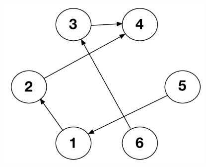
We can express these relationships using the adjacency matrix, , shown in Equation (52). Note that a in row of column indicates that a shock to will propagate to in the following period. Furthermore, we may model a shock to firm by post-multiplying by , where is a column vector of zeros with a one in the th row. If we wanted to determine the state of the financial system periods after the shock, we could compute this as .
| (52) |
While the problem we considered was intentionally stylized, computing for a large and can be computationally costly. Janzing and Wocjan (2006) demonstrate a superpolynomial speedup for problems of this form using a quantum algorithm. There are, however, several limitations of the algorithm:
-
1.
must be a symmetric matrix.
-
2.
must have fewer than polylog(N) non-zero entries per row, where is the number of columns.
-
3.
We must know the function, , which efficiently maps each row number to the row’s non-zero entry values.
-
4.
The number of exponentiations, , must be polylogarithmic in .
-
5.
It is only possible to examine diagonal elements, .
With respect to the fifth limitation, the algorithm only allows us to recover bounds on diagonal elements by testing whether or , where , and . Interested readers should see Janzing and Wocjan (2006) for the details of the algorithm’s implementation.
The authors stress that the algorithm is best suited to problems that can be reformulated in terms of a large, sparse matrix. This includes adjacency matrix problems of the style we considered earlier in this subsection, as long as they satisfy the aforementioned criteria. Furthermore, problems that involve large, sparse Markov transition matrices or fixed point algorithms may be able to exploit this routine. The most important limitation is that the research question will need to be answerable by testing bounds on a particular matrix diagonal element.
4.1.9 Quantum Annealing
This paper focuses primarily on “universal” quantum computers, which use the gate-circuit model of computation. In this section, however, we will discuss a specialized device called a “quantum annealer” that enables scaling with fewer technical difficulties. Whereas constructing a 50-qubit universal quantum computer is challenging with existing technology, commercially-available quantum annealers routinely make use of thousands of qubits. The most recently developed annealer (“Advantage”) offered by D-Wave Systems employs 5000 qubits.
In contrast to universal quantum computers, which can perform any computation, quantum annealers are exclusively capable of solving combinatorial optimization problems. This does, however, cover a large number of interesting and computationally-difficult problems in economics and finance. Indeed, recent work has shown that quantum annealers can solve small-scale versions of problems in finance, including the prediction of financial crises through the use of network models (Orús et al., 2019b; Ding et al., 2019). There has also been work in the physics literature that speculates on how quantum annealers could be used more generally to solve problems in finance (Orús et al., 2019a).
Quantum annealers use a process that is similar to adiabatic quantum computing, which converts combinational optimization problems into quadratic unconstrained binary optimization (QUBO) problems of the form given in Equation (53).
| (53) |
Note that and are given, and . is the Hamiltonian, which expresses the level of energy in the system, the lowest of which is called the “ground state.”
Adiabatic quantum computing works by embedding the weights, and , in a quantum system and then finding the ground state, which corresponds to the global minimum. The system is first initialized in the ground state for an arbitrary and trivial Hamiltonian, . The parameters of are then slowly changed until they become the parameters of – namely, and – as expressed in Equation (54).
| (54) |
According to the quantum adiabatic theorem, the Hamiltonian will remain in the ground state as long as the transition happens sufficiently slowly. Furthermore, theory provides us with a “speed limit,” below which the system will remain in the ground state, allowing us to find a global minimum. Importantly, however, the speed limit will not always have an analytical expression and may require exponential time.
While the quantum adiabatic theorem is instructive for understanding a process that is analogous to quantum annealing, commercially-available quantum annealers do not perform adiabatic quantum computing. In particular, they do not always remain in the ground state during the optimization process. It is also not generally believed that they are capable of solving NP-complete problems efficiently.
Although questions remain about the extent to which quantum annealers can provide a quantum advantage, it is clear that they can be applied to a large class of problems in economics and finance. In particular, any optimization problem that can be converted into a QUBO can also be run on a quantum annealer. For an extended overview of the quantum annealing literature, see Hauke et al. (2020).
4.1.10 Random Number Generation
Random numbers are frequently used in economics in simulation exercises and estimation routines. For most research applications, it is only important that the numbers generated satisfy statistical test requirements and can be reproduced. For this reason, research applications in economics and finance typically employ random number generators that come with common statistical packages. These are typically pseudo-random number generators (PRNGs) that do not use physical or “true” sources of randomness.
A commonly-used type of PRNG is the family of linear congruential generators introduced by Lehmer (1951). As described in Herrero-Collantes and Garcia-Escartin (2017), these use the recursive formula shown in Equation (55) to produce numbers that appear to be drawn from a uniform distribution. Such sequences can then be used to construct seemingly random draws from other commonly-used statistical distributions (Hörmann et al., 2004).
| (55) |
Note that , , and . Selecting , , and will determine the period of the generator and the quality of the randomness. Furthermore, is the modulo operator, which yields the remainder of . Figure VI compares a sequence of numbers generated randomly using standard parameters for a linear congruential generator with parameters selected sub-optimally for the algorithm. In addition to containing a visible, high-frequency period, the sequence with sub-optimally chosen parameter values has a sample mean that deviates from the uniform distribution’s mean by 10%.
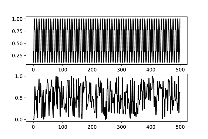
While such algorithms were once commonly used in statistical packages, they have recently been phased out in favor of the Mersenne Twister (MT) algorithm, introduced by Matsumoto and Nishimura (1998). For most applications in economics and finance, the linear congruential or MT algorithms are sufficient. Because linear congruential generators have been in widespread use for decades, there is a large literature documenting their failures. Herrero-Collantes and Garcia-Escartin (2017) provide a list of problems documented in this literature, including their tendency to cluster and become autocorrelated if a bad seed is selected.
Beyond pseudo-random number generators, there are also “physical” random number generators, which do not rely on algorithmic generation. These exploit random variation in the physical environment to generate a sequence of numbers or to select a seed for a PRNG. This might involve the use of random variation generated by a computer’s internal processes or user’s decisions, such as heat, noise, and mouse movements. Alternatively, it may instead rely on the use of random variation generated externally in the physical environment. One disadvantage of physical random number generation relative to PRNGs is that they cannot be reproduced from a seed and an algorithm. Instead, we must retain the set of numbers generated to achieve reproducibility. Due to the slow number generation rates for physical random number generation and the convenience and speed of PRNGs, physical random number generation has not gained widespread use for research applications within economics.
The approaches described above for physical RNG rely on classical physical processes, which are deterministic in nature. This is essentially the reason why “classical” physical RNG is so difficult: if nature is deterministic, where would the randomness come from? In contrast, quantum physics is probabilistic and, therefore, provides scope for generating randomness. We saw this in Figure I in Section 2, where we created a superposition and then performed measurement in the computational basis. This exact procedure can, in fact, be used to perform quantum random number generation (QRNG). Faster methods for QRNG involve the use of vacuum fluctuations, phase noise, and amplified spontaneous emission. We refer the interested reader to Herrero-Collantes and Garcia-Escartin (2017) for further detail.
QRNGs are one of the most mature quantum technologies. Beyond implementation within a quantum computing environment, they may also be generated by standalone, specialized quantum devices that are already commercially-available. Devices produced by ID Quantique, for instance, are small, easy-to-use, and affordable.585858In November of 2020, ID Quantique sold QRNG devices for roughly $1000. They have also recently been integrated into a smartphone that makes use true random number generation to provide enhanced security features.595959See https://www.idquantique.com. See Figure VII for an example of a standalone quantum random number generator.
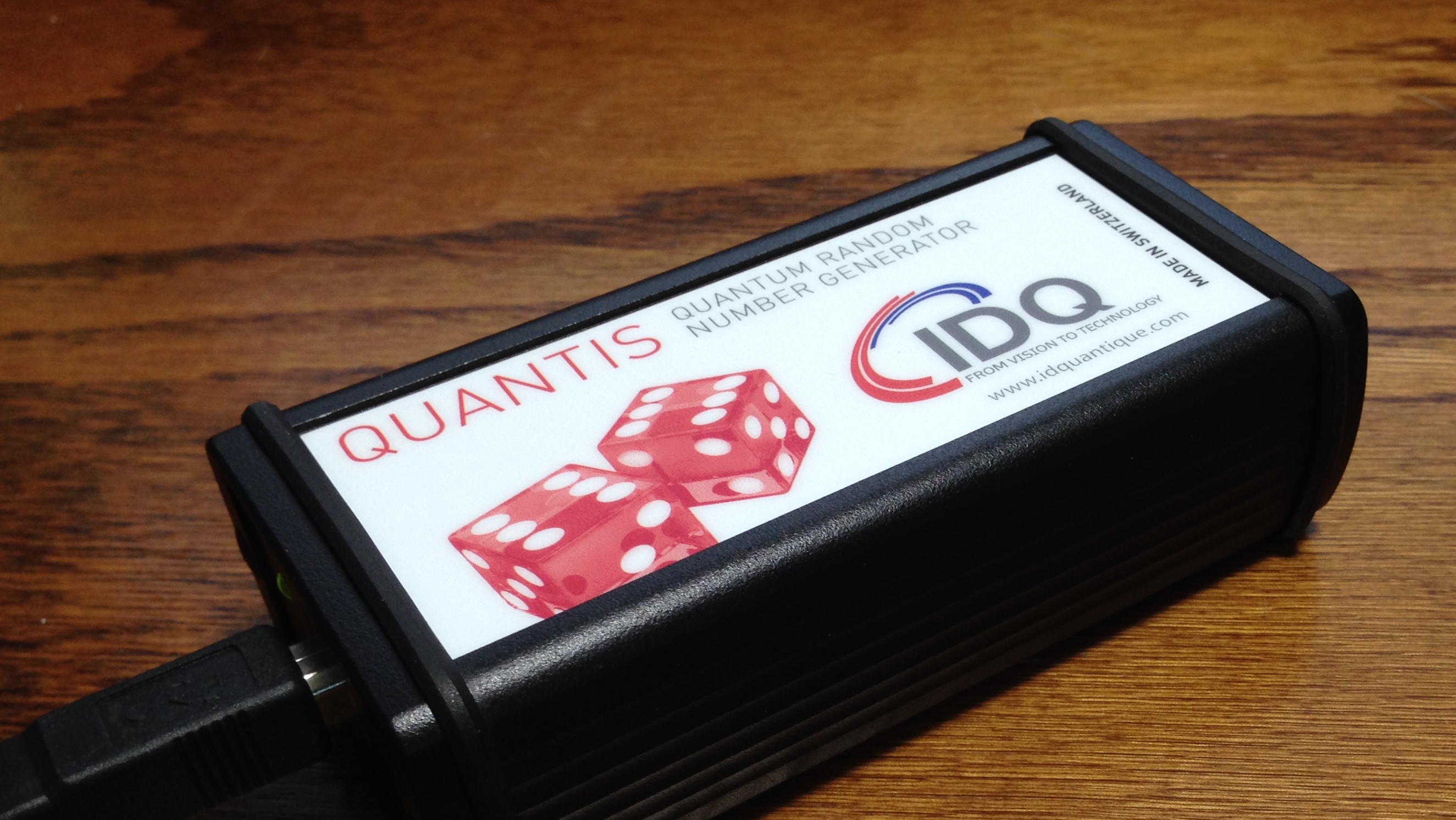
Relative to physical random number generators, QRNGs tend to perform generation faster, making them a more viable competitor for PRNG schemes. While MT-generated random numbers may be sufficient for most research problems in economics, QRNGs are likely to provide a compelling alternative that does not suffer from problems common to PRNGs.
An even stronger notion, called certified randomness, was recently introduced: one can generate randomness, starting from a short random seed, without trusting the quantum devices which generate the randomness. For an overview of the related literature, see Colbeck and Renner (2012), Vazirani and Vidick (2012), Miller and Shi (2016), Coudron and Yuen (2014), and Herrero-Collantes and Garcia-Escartin (2017).
4.2 Experimental Implementation
While there has been considerable progress in the development of quantum algorithms since the 1990s, much of the experimental progress has been realized more recently. In this subsection, we discuss the historical development of quantum computers, including the current state of progress. We also discuss the limits of what we can expect to achieve with quantum computation.
4.2.1 Experimental Progress in Quantum Computing
In 1982 Richard Feynman remarked that the world is not classical (Feynman, 1982),606060“Nature isn’t classical, dammit, and if you want to make a simulation of nature, you’d better make it quantum mechanical, and by golly it’s a wonderful problem, because it doesn’t look so easy.” and that quantum devices should be used for calculating properties of quantum systems at the microscopic level (Feynman, 1982, 1986). This triggered the beginning of an algorithmic (Barenco et al., 1995; Shor, 1994; Grover, 1996) and hardware-related (Monroe et al., 1995; Kielpinski et al., 2002; Makhlin et al., 2001; You et al., 2002) development that strongly influenced computational science and promised to revolutionize some lines of computation.
During the 1990s, ground-breaking work toward quantum computing with ion traps (Monroe et al., 1995) and molecular spins (Vandersypen et al., 2001) got a head start because of the previous development of atomic clocks and magnetic resonance imaging. From 2000, superconducting circuits (You et al., 2002; Makhlin et al., 2001) emerged as potential contenders for quantum computing through circuit quantum electrodynamics (cQED) (Wallraff et al., 2004) and Josephson-junction based qubits with long coherence times (Koch et al., 2007). There followed many advanced experiments and proofs-of-concept (Wineland, 2013; Blatt and Roos, 2012; Ansmann et al., 2009; DiCarlo et al., 2009) and a 2012 Nobel Prize in Physics. Nevertheless, only ten years ago a common opinion was that quantum computing was merely a distant possibility.
The basic reason for this pessimistic perspective was the need for quantum error correction (QEC), putting extreme demands on quantum hardware. However, in 2013 John Martinis’s group published a seminal paper (Barends et al., 2014) demonstrating basic operations with a five-qubit processor with error rates low enough for future successful fault-tolerant operation of the QEC surface code (Fowler et al., 2012). That work was followed by advanced operations with a nine-qubit chip (Barends et al., 2016) that ultimately became a fundamental building block in Google’s 54-qubit Sycamore chip (Arute et al., 2019).
There is now a broad effort to scale up devices and build large systems that should be able to challenge classical computers (Wendin, 2017). These scaled-up systems involve ion traps (Brown et al., 2016; Wright et al., 2019; Honeywell Quantum Solutions, 2020), superconducting circuits (Arute et al., 2019; IBM Quantum Computing, 2020; Rigetti Quantum, 2020; Alibaba Quatum Lab, 2020; Baidu Research, 2020; Andersen et al., 2019a, b; OpenSuperQ, 2020), optical traps for cold atomic gases (Gross and Bloch, 2017; Schweizer et al., 2019), and photonic circuits (Takeda and Furusawa, 2019). Semiconductor qubits are still at a proof-of-concept level (Watson et al., 2018), but the compatibility with standard silicon computer technology has lead to strong efforts to scale up to large systems (Li et al., 2018; Vandersypen and Eriksson, 2019). The present efforts to scale up different kinds of quantum hardware are necessarily putting strong focus on computer architecture for optimizing performance with respect to qubit coherence, connectivity, and integration (Matsuura et al., 2019).
So, what is the computational power and usefulness of these systems? Preskill introduced the concepts of quantum supremacy (Preskill, 2012) and noisy intermediate-scale quantum (NISQ) devices (Preskill, 2018). Quantum supremacy (or quantum advantage) is a computational regime in which quantum computers can perform at least one task orders of magnitude faster than classical high-performance computers (HPC).616161A “classical” computer is any computer that uses only classical operations, such as NAND, XOR, and OR gates in its computation. For example, our existing desktops are “classical” computers. In general, we will use the term “classical” to indicate that something is not quantum. It was speculated that quantum supremacy would initially be achieved using NISQ devices – the current vintage of quantum computers – which have enough qubits to challenge the performance of classical computers on certain tasks, but not enough to also provide quantum error correction.
The AI-group at Google published a paper in 2016 on how to characterize quantum supremacy in near-term devices with sampling of quantum random circuits (Boixo et al., 2018). Anticipating that quantum supremacy might be on the horizon, Aaronson and Chen (2017) then formalised the set of conditions that would need to be met in order to technically achieve it. They also identified tasks where quantum supremacy would most likely be achievable first. The viability of the Google random-circuit approach was verified by Bouland et al. (2019), and shortly afterwards Google published a paper in which they claimed to have achieved quantum supremacy by performing a computation in 200 seconds that would have taken 10,000 years on the world’s fastest classical supercomputer (Arute et al., 2019). This achievement was followed by a second demonstration of quantum supremacy by a group at the University of Science and Technology of China in Hefei (Zhong et al., 2020), which performed a boson sampling task times faster than would be possible on a state-of-the-art classical supercomputer.626262In contrast to Arute et al. (2019), Zhong et al. (2020) demonstrated quantum supremacy using a specialized quantum computing device that can only perform boson sampling.
IBM has argued (IBM, 2019) that the computation Google performed on its new quantum chip, Sycamore, could actually be performed in 2.5 days, rather than 10,000 years on IBM’s supercomputer, Summit, and that this classical performance could be further refined and sped up. The argument illuminates the floating division between classical performance and quantum supremacy (Pednault et al., 2017), as well as the usefulness and accuracy of quantum calculations. Adding a few more functional qubits to Sycamore would ensure that it surpasses any near-future HPC on the problem of sampling random quantum circuits when it comes to memory storage. However, that would also require many more, and higher-fidelity, operations on the quantum processing unit (QPU) to demonstrate quantum supremacy.
While the achievement of quantum supremacy marks an important milestone in the development of quantum computers, it does not imply that all tasks can now be more efficiently performed on quantum computers. Contrary to popular depictions, quantum computers are not simply classical computers with an expanded capacity for parallel computation. Rather, quantum computers allow us to compute with quantum physical resources, which require altogether different algorithms to perform the same tasks. Problems that can be directly mapped onto two-dimensional quantum spin systems – quantum magnets – can achieve a quantum speedup (Childs et al., 2018). However, there are, in fact, many computations that will almost certainly be more efficiently performed on classical computers in the foreseeable future. Furthermore, for many computational problems, there are no known quantum speedups and in some specific cases, it is possible to prove that no such speedups can be achieved.
It is also worth emphasizing that quantum computers are unlikely to be used as standalone substitutes for classical computers. Rather, it is more likely that they will be employed as quantum processing unit (QPU) accelerators in conjunction with classical computing systems, playing a role that is similar to that of graphical processing units (GPUs) or tensor processing units (TPUs).636363GPUs, which were originally developed to render graphics, have since been exploited to perform massively parallel computation of basic floating point operations. TPUs were developed to perform the computational function of a GPU, but without the capacity to render graphics. Had there not been substantial progress in the development of GPUs over the last decade, it is unlikely that machine learning would have experienced as much success as it has as a field. Similarly, it is possible that quantum computing could generate similar transformations by unlocking the solution and estimation of otherwise intractable models.
Currently, theoretical efforts and software development are focused toward near-term “use cases” – useful quantum computations on current and near-term NISQ QPUs. It can, of course, be discussed what is “useful”: Are fundamental physics problems useful or does usefulness imply a “real-life” problem? The issue with QPUs is that they are based on spin-like two-level or few-level systems (qubits, qutrits, qudits) and mapping problems onto qubit registers may be complicated. Spin systems map directly onto qubit registers, and many optimization problems are variational problems based on Ising type Hamiltonians and cost functions. A popular type of algorithm is the variational quantum approximate optimization algorithm (QAOA) (Farhi et al., 2014; Willsch et al., 2019; Vikstål et al., 2019; Bengtsson et al., 2019).
Variational quantum computing combines short bursts of quantum computation to execute quantum trial functions with classical pre- and post-processing of data (e.g. evaluating cost functions based on measurements for sampling of quantum trial functions). Currently, one applies the variational quantum eigensolver (VQE) algorithm (Peruzzo et al., 2014) to electron correlation problems in general, and quantum chemistry in particular (see e.g. Sokolov et al. (2020); Nam et al. (2020); Takeshita et al. (2019); Lolur et al. (2020)). The recipe for the quantum trial function is constructed classically by generating excitations from a molecular reference state, involving a large number of variational parameters to achieve chemical accuracy. Moreover, one must classically map fermionic operators to qubits via Jordan-Wigner-type transformations and construct the list of quantum gates describing the quantum circuit. The single, unique quantum step is the execution of the quantum gates that creates the quantum trial function in the multi-qubit register. The post-processing steps are all classical: measurements for sampling the trial state function, the calculation of expectations values, optimization, and iterative minimization. The rationale for the VQE is two-fold: (1) the quantum step is sufficiently hard in a classical setting so that the (classical) overhead will be unimportant in the end, and (2) the coherence time for the NISQ QPU is long enough for the quantum step to be executed.
The VQE was invented because the phase estimation algorithm (Cleve et al., 1998; Dobšíček et al., 2007) requires QPU coherence times far beyond what is possible in the NISQ era. The phase estimation algorithm scales much better than the VQE because it is essentially quantum all the way: it describes the time evolution from a classically defined initial quantum reference state under the action of the quantum Hamiltonian. There are no repeated measurements, optimization, and minimization – only final measurements and post-processing to find the energy of the molecular state. However, the quantum time evolution requires extremely long coherence times (i.e. a large number of quantum gate operations) in order to solve challenging problems and to establish quantum supremacy.
In practice, the VQE – and perhaps most classical-quantum hybrid schemes – also needs QPUs with extremely long coherence times for useful applications. Currently, the VQE can only be applied to fairly small molecules for proof-of-principle experimental demonstration of QC (Lolur et al., 2020). On the other hand, it provides a useful platform for benchmarking NISQ quantum hardware and for developing software and user interfaces. However, for establishing quantum supremacy, quantum error corrections schemes will be needed.
4.2.2 Limitations of Quantum Computing
Suppose we have access to some black-box function, , and our objective is to find an such that . This could be viewed as finding a needle (an such that ) in a haystack (of size ). Consider the following (naïve) algorithm: we first prepare a uniform superposition over all possible values using the Hadamard gate: . We then add another qubit register, and evaluate , so that the overall state is:
| (56) |
At this point, next to every , we have an . This might give the impression that we have almost solved the problem. Unfortunately, if we measure the last qubit, the probability of it being is . As such, we cannot expect to recover an for which is , even though there exists such an in the superposition. If there is exactly one needle in the haystack, we will to run this algorithm times to find a needle. Grover (1996) came up with a quantum algorithm that solves this using queries to , which is quadratically faster than the best classical algorithm, and the one we presented before.
We might wonder whether there is a better alternative that could provide more than a quadratic speedup. Unfortunately, Bennett et al. (1997) proved that Grover’s algorithm is optimal in the black-box model. Thus, quantum computers cannot solve the search problem exponentially faster than a classical computer. But what about other types of black-box problems? Could these be solved faster on a quantum computer? Unfortunately, this is also not the case: whatever black-box problem a quantum computer solves using queries, a classical computer could also solve using queries (Aaronson et al., 2020; Beals et al., 2001). Therefore, in order to get a super-polynomial speedup, we have to exploit some structure. This additional structure that the black-box satisfies is called a promise, and with a promise, we know that super-polynomial speedups can be achieved (see, e.g., Simon (1997) and Bernstein and Vazirani (1997)).
The discussion above centers on the black-box model; however, analysis in the standard model, without the black-box assumption, is harder, and there are more open problems and conjectures than answers. Consider, for example, the question of whether either classical or quantum computers can efficiently solve all problems – that is, all problems for which there is an efficient algorithm to verify a candidate proof. For example, a Sudoku puzzle has a valid solution, which can be efficiently verified given a candidate solution.646464Formally, this could be done in polynomial time in the size of the puzzle. It is conjectured that classical computers cannot efficiently solve all the problems in the class. This is known as the conjecture and is one of the Millennium Prize Problems (Carlson et al., 2006). It is also conjectured, partly based on the arguments that we discussed for the black-box model, that quantum computers also cannot efficiently solve all problems.
While substantial progress has been made in the development of quantum computers, it is worth emphasizing that quantum computing will not provide an exponential speedup for all algorithms, even after the production of quantum computers matures. Contrary to popular depictions, quantum superpositions do not allow for massive parallel computation in a trivial sense. Rather, quantum speedups typically rely on the subtle exploitation of quantum physics, rather than the brute force application of increased computational resources. This is why quantum speedups necessarily entail the development of quantum algorithms.
5 Conclusion
With Google claiming quantum supremacy (Arute et al., 2019), we have arguably crossed the threshold from one computational regime into another. Quantum computers went from a theoretical curiosity to the best available computational tool for at least one computational task. And while this change may seem sudden and unexpected, it followed a decade of steady progress in the development of quantum computers and was anticipated by the literature (Aaronson and Chen, 2017; Wendin, 2017). Quantum supremacy does not mean that all tasks will be performed more efficiently on quantum computers. Rather, it suggests that quantum computers have become sufficiently powerful that we can expect that a larger variety of computational tasks will eventually be most efficiently performed on them.
Our objective in this manuscript was to explain the implications of improvements in quantum technology, including quantum computers, for economists with the intention of drawing new voices into the existing dialogue with physicists, mathematicians, and computer scientists. As part of this effort, we have included both high-level explanations of concepts and also sufficient low-level detail to enable economists to construct literatures on quantum econometrics and quantum computational economics. We also attempted to clear up common misconceptions about quantum computers: No, quantum computers are not classical computers with an expanded capacity for parallelization. And no, quantum computers will not perform all computations exponentially faster than classical computers, but in certain cases, they will.
One implication of the development of powerful quantum computers is that the financial system may eventually come under quantum attack. Such attacks are categorically different from what can be done with classical computers, since sufficiently large quantum computers will be able to perform certain computationally tasks exponentially faster. Shor (1994), for instance, provides a near-exponential speedup to prime factorization, which compromises the RSA encryption algorithm. One solution to this problem is to employ post-quantum cryptography, which makes use of classical computers and classical algorithms, but employs cryptographic methods that are robust to both classical and quantum attack. Another option is to achieve security through the use quantum key distribution, which is one of the more mature quantum technologies and does not require the use of large quantum computers. In order to remain secure, forms of payment will need to be adapted to protect against such threats. Another possibility, which we examine, is to construct forms of money and payment instruments, broadly referred to as “quantum money,” which are robust to classical and quantum attacks.
Quantum money offers a bundle of features that is not achievable with physical cash or any digital currency scheme, including cryptocurrencies. In particular, quantum money is able to retain the beneficial features of a debit or credit transaction, including the ability to transact with minimal latency and at a distance, and the beneficial features of physical cash, such as the ability to transact offline and without the involvement of a trusted third party. It also achieves a higher level of security than is possible with any classical scheme. Furthermore, quantum money can also be issued and maintained by a central bank, which means that conventional monetary policy could be applied.
While quantum money remains technologically infeasible to implement at scale in the short-run, there has been substantial experimental progress in the past few years, including the partial implementation of quantum money and quantum credit cards. No public-key scheme has yet been implemented experimentally; and even the theoretical construction of such schemes remains a formidable analytical challenge. However, the benefits of implementing a public-key scheme would be substantial: it would allow for the possibility of combining both the anonymity and privacy of physical cash and the benefits that digital payment systems have introduced.
Finally, we conducted an exhaustive review of quantum algorithms that could potentially be used to solve or estimate economic models. We identify more than ten categories of algorithms that could provide quantum speedups to solution and estimation routines. In many cases, the quantum versions of the routines face limitations that were not present in the classical version. This is partly the result of quantum computers achieving speedups through the subtle exploitation of quantum physical phenomena, rather than brute-force parallelization. We also saw that phase kickback, phase estimation, and quantum Fourier transforms (QFTs) were common ingredients in algorithms that managed to achieve such speedups.
6 Acknowledgements
G.W. is supported by the European Commission through project 820363: OpenSuperQ, and by the Knut and Alice Wallenberg (KAW) foundation and Chalmers University of Technology through the WACQT project. E.D. is supported by the French National Research Agency through the project ANR-17-CE39-0005 quBIC. And O.S. is supported by the Israeli Science Foundation (ISF) grant No. 682/18 and 2137/19, and by the Cyber Security Research Center at Ben-Gurion University.
References
- (1)
- Aaronson (2009) Aaronson, S. (2009) “Quantum Copy-Protection and Quantum Money,” Conference on Computational Complexity, Vol. IEEE, pp. 229–242, DOI: 10.1109/ccc.2009.42.
- Aaronson (2015) (2015) “Read the Fine Print,” Nature Physics, Vol. 11, pp. 291–293, DOI: 10.1038/nphys3272.
- Aaronson and Chen (2017) Aaronson, S. and L. Chen (2017) “Complexity-Theoretic Foundations of Quantum Supremacy Experiments,” in O’Donnell, R. ed. 32nd Computational Complexity Conference, CCC 2017, July 6-9, 2017, Riga, Latvia, Vol. 79 of LIPIcs, pp. 22:1–22:67: Schloss Dagstuhl - Leibniz-Zentrum fuer Informatik, URL: https://doi.org/10.4230/LIPIcs.CCC.2017.22, DOI: 10.4230/LIPIcs.CCC.2017.22.
- Aaronson and Christiano (2012) Aaronson, S. and P. Christiano (2012) “Quantum Money from Hidden Subspaces,” Proceedings of the 44th Symposium on Theory of Computing, Vol. ACM, pp. 41–60, DOI: 10.1145/2213977.2213983.
- Aaronson et al. (2020) Aaronson, S., S. Ben-David, R. Kothari, and A. Tal (2020) “Quantum Implications of Huang’s Sensitivity Theorem.”
- Ackerberg (2003) Ackerberg, D. (2003) “Advertising, Learning, and Consumer Choice in Experience Good Markets: An Empirical Examination,” International Economic Review, Vol. 44, pp. 1007–1040, URL: https://www.jstor.org/stable/3663546.
- Aggarwal et al. (2018) Aggarwal, S., G. Brennen, T. Lee, M. Santha, and M. Tomamichel (2018) “Quantum Attacks on Bitcoin, and How to Protect Against Them,” Ledger, Vol. 3, DOI: 10.5195/ledger.2018.127.
- Aguirregabiria and Mira (2002) Aguirregabiria, V. and P. Mira (2002) “Swapping the Nested Fixed Point Algorithm: A Class of Estimators for Discrete Markov Decision Models,” Econometrica, Vol. 70, pp. 1519–1543, URL: https://www.jstor.org/stable/3082006.
- Aguirregabiria and Mira (2010) (2010) “Dynamic Discrete Choice Structural Models: A Survey,” Journal of Econometrics, Vol. 156, pp. 38–67, DOI: 10.1016/j.jeconom.2009.09.007.
- Ahmadi and Chiang (2012) Ahmadi, H. and C. Chiang (2012) “Quantum Phase Estimation with Arbitrary Constant-Precision Phase Shift Operators,” Quantum Information & Computation, Vol. 12, No. 9-10, pp. 864–875, URL: http://dl.acm.org/citation.cfm?id=2481580.2481589.
- Aiyagari (1994) Aiyagari, R. (1994) “Uninsured Idiosyncratic Risk and Aggregate Saving,” The Quarterly Journal of Economics, Vol. 109, No. 3, pp. 659–684, DOI: 10.2307/2118417.
- Albert and Chib (1993) Albert, J. and S. Chib (1993) “Bayes Inference via Gibbs Sampling of Autoregressive Time Series Subject to Markov Mean and Variance Shifts,” Journal of Business and Economic Statistics, Vol. 11, pp. 1–5, DOI: 10.2307/1391303.
- Aleklett et al. (1981) Aleklett, K., D. Morrissey, W. Loveland, P. McGaughey, and G. Seaborg (1981) “Energy dependence of fragmentation in relativistic nuclear collisions,” Phys. Rev. C, Vol. 23, pp. 1044–1046, URL: https://link.aps.org/doi/10.1103/PhysRevC.23.1044, DOI: 10.1103/PhysRevC.23.1044.
- Alibaba Quatum Lab (2020) Alibaba Quatum Lab (2020) , URL: https://damo.alibaba.com/labs/quantum.
- Ambainis (2010) Ambainis, A. (2010) “Variable Time Amplitude Amplification and a Faster Quantum Algorithm for Solving Systems of Linear Equations,” Working Paper. URL: https://arxiv.org/abs/1010.4458.
- Amiri and Arrazola (2017) Amiri, R. and J. Arrazola (2017) “Quantum money with nearly optimal error tolerance,” Physical Review A, Vol. 95, No. 6, DOI: 10.1103/physreva.95.062334.
- Amos et al. (2020) Amos, R., M. Georgiou, A. Kiayias, and M. Zhandry (2020) “One-shot Signatures and Applications to Hybrid Quantum/Classical Authentication,” in Proceedings of STOC 2020.
- Anand et al. (2012) Anand, K., P. Gai, and M. Marsili (2012) “Rollover Risk, Network Structure and Systemic Financial Crises,” Journal of Economic Dynamics and Control, Vol. 36, pp. 1088–1100, DOI: 10.1016/j.jedc.2012.03.005.
- Andersen et al. (2019a) Andersen, C. et al. (2019a) “Entanglement stabilization using ancilla-based parity detection and real-time feedback in superconducting circuits,” npj Quantum Information, Vol. 5, No. 1, p. 69, DOI: 10.1038/s41534-019-0185-4.
- Andersen et al. (2019b) (2019b) “Repeated Quantum Error Detection in a Surface Code,” Working paper. URL: https://arxiv.org/pdf/1912.09410.pdf.
- Andersen et al. (2001) Andersen, T., T. Bollerslev, F. Diebold, and H. Ebens (2001) “The Distribution of Realized Stock Return Volatility,” Journal of Financial Economics, Vol. 61, No. 1, pp. 43–76, DOI: 10.1016/S0304-405X(01)00055-1.
- Ansmann et al. (2009) Ansmann, M. et al. (2009) “Violation of Bell’s inequality in Josephson phase qubits,” Nature, Vol. 461, No. 7263, pp. 504–506, DOI: 10.1038/nature08363.
- Anufriev and Panchenko (2015) Anufriev, M. and V. Panchenko (2015) “Connecting the Dots: Econometric Methods for Uncovering Networks with an Application to the Australia Financial Institutions,” Journal of Banking and Finance, Vol. 61, pp. 241–255, DOI: 10.1016/j.jbankfin.2015.08.034.
- Arrazola et al. (2016) Arrazola, J., M. Karasamanis, and N. Lütkenhaus (2016) “Practical Quantum Retrieval Games,” Phys. Rev. A, Vol. 93, No. 062311, DOI: 10.1103/PhysRevA.93.062311.
- Aruoba et al. (2006) Aruoba, S., J. Fernández-Villaverde, and J. Rubio-Ramirez (2006) “Comparing Solution Methods for Dynamic Equilibrium Economies,” Journal of Economic Dynamics and Control, Vol. 30, No. 12, pp. 2477–2508, URL: http://dx.doi.org/10.2139/ssrn.488845.
- Arute et al. (2019) Arute, F. et al. (2019) “Quantum Supremacy Using a Programmable Superconducting Processor,” Nature, Vol. 574, pp. 505––510, DOI: 10.1038/s41586-019-1666-5.
- Bae et al. (2003) Bae, K.-H., G. Karolyi, and R. Stulz (2003) “A New Approach to Measuring Financial Contagion,” The Review of Financial Studies, Vol. 16, pp. 717–763, DOI: 10.1093/rfs/hhg012.
- Bai (2003) Bai, J. (2003) “Inferential Theory for Factor Models of Large Dimensions,” Econometrica, Vol. 71, No. 1, pp. 135–171, DOI: 10.1111/1468-0262.00392.
- Baidu Research (2020) Baidu Research (2020) , URL: http://research.baidu.com/Research_Areas/index-view?id=75.
- Ballester et al. (2006) Ballester, C., A. Calvó-Armengol, and Y. Zenou (2006) “Who’s Who in Networks. Wanted: The Key Player,” Econometrica, Vol. 74, pp. 1403–1417, URL: https://www.jstor.org/stable/3805930.
- Bar-Yossef et al. (2004) Bar-Yossef, Z., T. Jayram, and I. Kerenidis (2004) “Exponential Separation of Quantum and Classical One-Way Communication Complexity,” Proceedings of the 36th Symposium on Theory of Computing, pp. 128–137, DOI: 10.1145/1007352.1007379.
- Barenco et al. (1995) Barenco, A. et al. (1995) “Elementary Gates for Quantum Computation,” Phys. Rev. A, Vol. 52, pp. 3457–3467, DOI: 10.1103/PhysRevA.52.3457.
- Barends et al. (2014) Barends, R. et al. (2014) “Superconducting quantum circuits at the surface code threshold for fault tolerance,” Nature, Vol. 508, No. 7497, pp. 500–503, DOI: 10.1038/nature13171.
- Barends et al. (2016) (2016) “Digitized adiabatic quantum computing with a superconducting circuit,” Nature, Vol. 534, No. 7606, pp. 222–226, DOI: 10.1038/nature17658.
- Bargigli and Gallegati (2011) Bargigli, L. and M. Gallegati (2011) “Random Digraphs with Given Expected Degree Sequences: A Model for Economic Networks,” Journal of Economic Behavior and Organization, Vol. 78, pp. 396–411, DOI: 10.1016/j.jebo.2011.01.022.
- Bartkiewicz et al. (2017) Bartkiewicz, K. et al. (2017) “Experimental Quantum Forgery of Quantum Optical Money,” npj Quantum Information, Vol. 7, DOI: 10.1038/s41534-017-0010-x.
- Beals et al. (2001) Beals, R. et al. (2001) “Quantum lower bounds by polynomials,” J. ACM, Vol. 48, No. 4, pp. 778–797, DOI: 10.1145/502090.502097.
- Behera and Sattath (2020) Behera, A. and O. Sattath (2020) “Almost Public Coins.”
- Behera et al. (2017) Behera, B., T. Banerjee, and P. Panigrahi (2017) “Experimental Realization of Quantum Cheque Using a Five-Qubit Quantum Computer,” Quantum Information Processing, Vol. 16, No. 12, DOI: 10.1007/s11128-017-1762-0.
- Bell (1964) Bell, J. (1964) “On the Einstein Podolsky Rosen Paradox,” Physics, Vol. 1, No. 3, pp. 195–200, DOI: 10.1103/PhysicsPhysiqueFizika.1.195.
- Belsley (1980) Belsley, D. (1980) “On the Efficient Computation of the Nonlinear Full-Information Maximum-Likelihood Estimator,” Journal of Econometrics, Vol. 14, pp. 203–225, DOI: 10.1016/0304-4076(80)90091-3.
- Ben-David and Sattath (2016) Ben-David, S. and O. Sattath (2016) “Quantum Tokens for Digital Signatures.”
- Bengtsson et al. (2019) Bengtsson, A. et al. (2019) “Quantum approximate optimization of the exact-cover problem on a superconducting quantum processor,” Working paper. URL: https://arxiv.org/pdf/1912.10495.pdf.
- Bennett et al. (1982) Bennett, C., S. Brassard, S. Breidbart, and S. Wiesner (1982) “Quantum Cryptography, or Unforgeable Subway Tokens,” Advances in Cryptology, pp. 267–275, DOI: 10.1007/978-1-4757-0602-4_26.
- Bennett et al. (1997) Bennett, C. H., E. Bernstein, G. Brassard, and U. V. Vazirani (1997) “Strengths and Weaknesses of Quantum Computing,” SIAM J. Comput., Vol. 26, No. 5, pp. 1510–1523, URL: https://doi.org/10.1137/S0097539796300933, DOI: 10.1137/S0097539796300933.
- Bernanke et al. (2005) Bernanke, B., J. Boivin, and P. Eliasz (2005) “Measuring the Effects of Monetary Policy: A Factor-Augmented Vector Autoregressive (FAVAR) Approach,” Quarterly Journal of Economics, Vol. 120, No. 1, pp. 387–422, URL: https://www.jstor.org/stable/25098739.
- Berndt et al. (1974) Berndt, E., B. Hall, R. Hall, and J. Hausman (1974) “Estimation and Inference in Nonlinear Structural Models,” Annals of Economic and Social Measurement, Vol. 3, pp. 653–665.
- Bernstein and Vazirani (1997) Bernstein, E. and U. V. Vazirani (1997) “Quantum Complexity Theory,” SIAM J. Comput., Vol. 26, No. 5, pp. 1411–1473, URL: https://doi.org/10.1137/S0097539796300921, DOI: 10.1137/S0097539796300921.
- Bewley (1977) Bewley, T. (1977) “The Permanent Income Hypothesis: A Theoretical Formulation,” Journal of Economic Theory, Vol. 16, pp. 252–292, DOI: 10.1016/0022-0531(77)90009-6.
- Biamonte et al. (2017) Biamonte, J., P. Wittek, N. Pancotti, P. Rebentrost, N. Wiebe, and S. Lloyd (2017) “Quantum Machine Learning,” Nature, Vol. 549, pp. 195–202, DOI: 10.1038/nature23474.
- Billio et al. (2012) Billio, M., M. Getmansky, A. Lo, and P. Loriana (2012) “Econometric Measures of Connectedness and Systemic Risk in the Finance and Insurance Sectors,” Journal of Financial Economics, Vol. 104, No. 3, pp. 535–559, DOI: 10.1016/j.jfineco.2011.12.010.
- Blanchard and Kahn (1980) Blanchard, O. and C. Kahn (1980) “The Solution of Linear Difference Models Under Rational Expectations,” Econometrica, Vol. 48, pp. 1305–1311, DOI: 10.2307/1912186.
- Blatt and Roos (2012) Blatt, R. and C. Roos (2012) “Quantum simulations with trapped ions,” Nature Physics, Vol. 8, No. 4, pp. 277–284, DOI: 10.1038/nphys2252.
- Blin and Murphy (1974) Blin, J. and F. Murphy (1974) “On Measuring Economic Interrelatedness,” The Review of Economic Studies, Vol. 41, No. 3, pp. 437–440, DOI: 10.2307/2296761.
- Blundell et al. (2008) Blundell, R., L. Pistaferri, and I. Preston (2008) “Consumption Inequality and Partial Insurance,” American Economic Review, Vol. 98, No. 5, pp. 1887–1921, DOI: 10.1257/aer.98.5.1887.
- Böhme et al. (2015) Böhme, C., N. Christin, B. Edelman, and T. Moore (2015) “Bitcoin: Economics, Technology, and Governance,” Journal of Economic Perspectives, Vol. 29, No. 2, pp. 213–238, DOI: 10.1257/jep.29.2.213.
- Boivin and Ng (2006) Boivin, J. and S. Ng (2006) “Are More Data Always Better for Factor Analysis?” Journal of Econometrics, Vol. 132, No. 1, pp. 169–194, DOI: 10.1016/j.jeconom.2005.01.027.
- Boixo et al. (2018) Boixo, S. et al. (2018) “Characterizing quantum supremacy in near-term devices,” Nature Physics, Vol. 14, No. 6, pp. 595–600.
- Bollerslev (1986a) Bollerslev, T. (1986a) “Generalized Autoregressive Conditional Heteroskedasticity,” Journal of Econometrics, Vol. 31, pp. 307–327, DOI: 10.1016/0304-4076(86)90063-1.
- Bollerslev (1986b) (1986b) “Generalized Autoregressive Conditional Heteroskedasticity,” Journal of Econometrics, Vol. 31, pp. 307–327, DOI: 10.1016/0304-4076(86)90063-1.
- Bollerslev (1987) (1987) “A Conditionally Heteroskedastic Time Series Model for Speculative Prices and Rates of Return,” Journal of Econometrics, Vol. 69, pp. 542–547, DOI: 10.2307/1925546.
- Bollerslev et al. (2013) Bollerslev, T., V. Todorov, and S. Li (2013) “Jump Tails, Extreme Dependencies, and the Distribution of Stock Returns,” Journal of Econometrics, Vol. 172, No. 2, pp. 307–324, DOI: 10.1016/j.jeconom.2012.08.014.
- Bordo and Levin (2017) Bordo, M. and A. Levin (2017) “Central Bank Digital Currency and the Future of Monetary Policy,” Working Paper No. 23711, NBER.
- Born (1926) Born, M. (1926) “On the Quantum Mechanics of Collisions,” Zeitschrift für Physik, Vol. 37, pp. 863–867.
- Bouland et al. (2019) Bouland, A., B. Fefferman, C. Nirkhe, and U. Vazirani (2019) “On the complexity and verification of quantum random circuit sampling,” Nature Physics, Vol. 15, No. 2, pp. 159–163, DOI: 10.1038/s41567-018-0318-2.
- Bouland et al. (2020) Bouland, A., W. van Dam, H. Joorati, I. Kerenidis, and A. Prakash (2020) “Prospects and challenges of quantum finance.”
- Bozzio et al. (2018) Bozzio, M. et al. (2018) “Experimental Investigation of Practical Unforgeable Quantum Money,” npj Quantum Information, Vol. 4, No. 5, DOI: 10.1038/s41534-018-0058-2.
- Bozzio (2019) Bozzio, M. (2019) Security and implementation of advanced quantum cryptography: quantum money and quantum weak coin flipping Ph.D. dissertation, Paris.
- Bozzio et al. (2019) Bozzio, M., E. Diamanti, and F. Grosshans (2019) “Semi-device-independent quantum money with coherent states,” Physical Review A, Vol. 99, p. 022336.
- Brassard et al. (2002) Brassard, G., P. Høyer, M. Mosca, and A. Tapp (2002) “Quantum Amplitude Amplification and Estimation,” Quantum Computation and Quantum Information: A Millennium Volume, pp. 53–74.
- Bravyi et al. (2011) Bravyi, S., A. Harrow, and A. Hassidim (2011) “Quantum Algorithms for Testing Properties of Distributions,” IEEE Transactions on Information Theory, Vol. 57, No. 6, pp. 3971–3981, DOI: 10.1109/TIT.2011.2134250.
- Brown et al. (2016) Brown, K., J. Kim, and C. Monroe (2016) “Co-designing a scalable quantum computer with trapped atomic ions,” npj Quantum Information, Vol. 2, No. 1, p. 16034, DOI: 10.1038/npjqi.2016.34.
- Bulger (2005) Bulger, D. (2005) “Quantum Basin Hopping with Gradient-Based Local Optimisation,” Working Paper. URL: https://arxiv.org/abs/quant-ph/0507193.
- Bunch (1988) Bunch, D. (1988) “A Comparison of Algorithms for Maximum Likelihood Estimation of Choice Models,” Journal of Econometrics, Vol. 38, pp. 145–167, DOI: 10.1016/0304-4076(88)90031-0.
- Burtless and Hausman (1978) Burtless, G. and J. Hausman (1978) “The Effect of Taxation on Labor Supply: Evaluating the Gary Negative Income Tax Experiment,” Journal of Political Economy, Vol. 86, pp. 1103–1130, URL: https://www.jstor.org/stable/1840399.
- Carlson et al. (2006) Carlson, J., A. Jaffe, and A. Wiles eds. (2006) The Millennium Prize Problems: Clay Mathematics Institute, Cambridge, MA; American Mathematical Society, Providence, RI, pp.xviii+165.
- Carroll and Samwick (1998) Carroll, C. and A. Samwick (1998) “How Important is Precautionary Saving?” Econometrica, Vol. 80, No. 3, pp. 410–419, URL: https://www.jstor.org/stable/2646749.
- Castanias (1979) Castanias, R. (1979) “Macroinformation and the Variability of Stock Market Prices,” The Journal of Finance, Vol. 34, No. 2, pp. 439–450, DOI: 10.2307/2326984.
- Catalini and Gans (2019) Catalini, C. and J. Gans (2019) “Some Simple Economics of the Blockchain,” Research Paper No. 5191-16, MIT Sloan.
- Chatterjee et al. (2007) Chatterjee, S., D. Corbae, M. Nakajima, and J. Ríos-Rull (2007) “A Quantitative Theory of Unsecured Consumer Credit with Risk of Default,” Econometrica, Vol. 75, No. 6, pp. 1525–1589, DOI: 10.1111/j.1468-0262.2007.00806.x.
- Chen et al. (2017) Chen, J., A. Childs, and S.-H. Hung (2017) “Quantum Algorithm for Multivariate Polynomial Interpolation,” Proceedings of the Royal Society A, Vol. 474, DOI: 10.1098/rspa.2017.0480.
- Chib (1993) Chib, S. (1993) “Bayes Regression with Autocorrelated Errors: A Gibbs Sampling Approach,” Journal of Econometrics, Vol. 58, pp. 275–294, DOI: 10.1016/0304-4076(93)90046-8.
- Chib et al. (2002) Chib, S., F. Nardari, and N. Shephard (2002) “Markov Chain Monte Carlo Methods for Stochastic Volatility Models,” Journal of Econometrics, Vol. 108, pp. 281–316, DOI: 10.1016/S0304-4076(01)00137-3.
- Childs (2017) Childs, A. (2017) “Lecture Notes on Quantum Algorithms.”
- Childs et al. (2016) Childs, A., W. van Dam, S. Hung, and I. Shparlinski (2016) “Optimal Quantum Algorithm for Polynomial Interpolation,” in Chatzigiannakis, I., M. Mitzenmacher, Y. Rabani, and D. Sangiorgi eds. 43rd International Colloquium on Automata, Languages, and Programming (ICALP 2016), pp. 1–13, Germany: Schloss Dagstuhl- Leibniz-Zentrum fur Informatik GmbH, Dagstuhl Publishing, 8, DOI: 10.4230/LIPIcs.ICALP.2016.16.
- Childs et al. (2018) Childs, A. et al. (2018) “Toward the first quantum simulation with quantum speedup,” Proceedings of the National Academy of Sciences, Vol. 115, No. 38, pp. 9456–9461, URL: https://www.pnas.org/content/115/38/9456, DOI: 10.1073/pnas.1801723115.
- Childs et al. (2017) Childs, A., R. Kothari, and R. Somma (2017) “Quantum Algorithm for Systems of Linear Equations with Exponentially Improved Dependence on Precision,” SIAM Journal on Computing, Vol. 46, pp. 1920–1950, DOI: 10.1137/16M1087072.
- Chiu and Koeppl (2017) Chiu, J. and T. Koeppl (2017) “The Economics of Cryptocurrencies – Bitcoin and Beyond,” working paper, SSRN, http://dx.doi.org/10.2139/ssrn.3048124.
- Christian et al. (2011) Christian, L., M. Trabandt, and K. Walentin (2011) “Introducing Financial Frictions and Unemployment into a Small Open Economy Model,” Journal of Economic Dynamics and Control, Vol. 35, pp. 1999–2041, DOI: 10.1016/j.jedc.2011.09.005.
- Christoffel et al. (2010) Christoffel, K., G. Coenen, and A. Warne (2010) “Forecasting with DSGE Models,” Working Paper No. 1185, ECB, https://www.doi.org/10.1093/oxfordhb/9780195398649.013.0005.
- Cleve et al. (1998) Cleve, R., A. Ekert, C. Macchiavello, and M. Mosca (1998) “Quantum algorithms revisited,” Proceedings of the Royal Society of London. Series A: Mathematical, Physical and Engineering Sciences, Vol. 454, No. 1969, p. 339–354, DOI: 10.1098/rspa.1998.0164.
- Coladangelo and Sattath (2020) Coladangelo, A. and O. Sattath (2020) “A Quantum Money Solution to the Blockchain Scalability Problem.”
- Colbeck and Renner (2012) Colbeck, R. and R. Renner (2012) “Free Randomness Can Be Amplified,” Nature Physics, Vol. 8, No. 6, pp. 450–453, DOI: 10.1038/nphys2300.
- Collin-Dufresne et al. (2001) Collin-Dufresne, P., R. Goldstein, and J. Martin (2001) “The Determinants of Credit Spread Changes,” Journal of Finance, Vol. 56, No. 6, pp. 2177–2207, URL: https://www.jstor.org/stable/2697820.
- Conde Pena et al. (2019) Conde Pena, M., R. Durán Díaz, J. Faugère, L. Hernández Encinas, and L. Perret (2019) “Non-quantum cryptanalysis of the noisy version of Aaronson–Christiano’s quantum money scheme,” IET Information Security, Vol. 13, No. 4, pp. 362–366.
- Conrad et al. (2013) Conrad, J., R. Dittmar, and E. Ghysels (2013) “Ex Ante Skewness and Expected Stock Returns,” The Journal of Finance, Vol. 68, No. 1, pp. 85–124, DOI: 10.1111/j.1540-6261.2012.01795.x.
- Coudron and Yuen (2014) Coudron, M. and H. Yuen (2014) “Infinite Randomness Expansion with a Constant Number of Devices,” in Shmoys, D. ed. Symposium on Theory of Computing, STOC 2014, New York, NY, USA, May 31 - June 03, 2014, pp. 427–436: ACM, DOI: 10.1145/2591796.2591873.
- Crawford and Shum (2005) Crawford, G. and M. Shum (2005) “Uncertainty and Learning in Pharmaceutical Demand,” Econometrica, Vol. 73, pp. 1137–1173, DOI: 10.1111/j.1468-0262.2005.00612.x.
- Danielsson (1994) Danielsson, J. (1994) “Stochastic Volatility in Asset Prices Estimation with Simulated Maximum Likelihood,” Journal of Econometrics, Vol. 64, pp. 375–400, DOI: 10.1016/0304-4076(94)90070-1.
- Davidson and MacKinnon (1993) Davidson, R. and J. MacKinnon (1993) Estimation and Inference in Econometrics: Oxford University Press.
- De Santis and Gérard (1997) De Santis, G. and B. Gérard (1997) “International Asset Pricing and Portfolio Diversification with Time-Varying Risk,” The Journal of Finance, Vol. 52, pp. 1881–1912, URL: https://www.jstor.org/stable/2329468.
- De Santis and Gérard (1998) De Santis, G. and B. Gérard (1998) “How Big is the Premium for Currency Risk?” Journal of Financial Economics, Vol. 49, pp. 375–412, DOI: 10.1016/S0304-405X(98)00029-4.
- Degen et al. (2017) Degen, C., F. Reinhard, and P. Cappellaro (2017) “Quantum sensing,” Rev. Mod. Phys., Vol. 89, p. 035002, DOI: 10.1103/RevModPhys.89.035002.
- Deutsch and Jozsa (1992) Deutsch, D. and R. Jozsa (1992) “Rapid Solution of Problems by Quantum Computation,” Proceedings of the Royal Society of London Series A, Vol. 493, pp. 553–558, DOI: 10.1098/rspa.1992.0167.
- DiCarlo et al. (2009) DiCarlo, L. et al. (2009) “Demonstration of two-qubit algorithms with a superconducting quantum processor,” Nature, Vol. 460, pp. 240–244, DOI: 10.1038/nature08121.
- Diebold and Yilmaz (2014) Diebold, F. and K. Yilmaz (2014) “On the Network Topology of Variance Decompositions: Measuring the Connectedness of Financial Firms,” Journal of Econometrics, Vol. 182, pp. 119–134, DOI: 10.1016/j.jeconom.2014.04.012.
- Dillaye (1877) Dillaye, S. (1877) Assignats and Mandats: A True History, Including an Examination of Dr. Andrew D. White’s ”Paper Money Inflation in France”, Pamphlets in American history: Finance: Philadelphia: Henry Carey Baird & Co.
- Ding et al. (2019) Ding, Y. et al. (2019) “Towards Prediction of Financial Crashes with a D-Wave Quantum Computer,” Working paper. URL: https://arxiv.org/pdf/1904.05808.pdf.
- Dirac (1939) Dirac, P. (1939) “A New Notation for Quantum Mechanics,” Mathematical Proceedings of the Cambridge Philosophical Society, Vol. 35, pp. 416–418, DOI: 10.1017/S0305004100021162.
- Dobšíček et al. (2007) Dobšíček, M., G. Johansson, V. Shumeiko, and G. Wendin (2007) “Arbitrary accuracy iterative quantum phase estimation algorithm using a single ancillary qubit: A two-qubit benchmark,” Physical Review A, Vol. 76, p. 030306, DOI: 10.1103/PhysRevA.76.030306.
- Dufour and Engle (2000) Dufour, A. and R. Engle (2000) “Time and the Price Impact of a Trade,” The Journal of Finance, Vol. 55, pp. 2467–2498, DOI: 10.1111/0022-1082.00297.
- Dutta et al. (2018) Dutta, S. et al. (2018) “Demonstration of a Quantum Circuit Methodology for Multiple Regression,” working paper, https://arxiv.org/abs/1811.01726.
- Dwyer (2015) Dwyer, G. (2015) “The Economics of Bitcoin and Similar Private Digital Currencies,” Journal of Financial Stability, Vol. 17, pp. 81–91, DOI: 10.1016/j.jfs.2014.11.006.
- Dyhrberg (2016) Dyhrberg, A. (2016) “Bitcoin, Gold, and the Dollar - A GARCH Volatility Analysis,” Finance Research Letters, Vol. 16, pp. 85–92, DOI: 10.1016/j.frl.2015.10.008.
- Egger et al. (2020) Egger, D. J. et al. (2020) “Quantum computing for Finance: state of the art and future prospects,” DOI: 10.1109/TQE.2020.3030314.
- Einstein et al. (1935) Einstein, A., B. Podolsky, and N. Rosen (1935) “Can Quantum-Mechanical Description of Physical Reality Be Considered Complete?” Physical Review, Vol. 47, DOI: 10.1103/PhysRev.47.777.
- Engel (2000) Engel, R. (2000) “The Econometrics of Ultra-High-Frequency Data,” Econometrica, Vol. 68, pp. 1–22, URL: https://www.jstor.org/stable/2999473.
- Engle et al. (1987) Engle, R., D. Lilien, and R. Robins (1987) “Estimating Time Varying Risk Premia in the Term Structure: The Arch-M Model,” Econometrica, Vol. 55, pp. 391–407, DOI: 10.2307/1913242.
- Engle and Russell (1998) Engle, R. and J. Russell (1998) “Autoregressive Conditional Duration: A New Model for Irregularly Spaced Transaction Data,” Econometrica, Vol. 66, pp. 1127–1162, DOI: 10.2307/2999632.
- Epps and Epps (1976) Epps, T. and M. Epps (1976) “The Stochastic Dependence of Security Price Changes and Transaction Volumes: Implications from Mixture-of-Distributions Hypothesis,” Econometrica, Vol. 44, No. 2, pp. 305–321, DOI: 10.2307/1912726.
- Farhi et al. (2012) Farhi, E. et al. (2012) “Quantum Money from Knots,” Proceedings of the 3rd Innovations in Theoretical Computer Science Conference, Vol. ACM, No. 276-289.
- Farhi et al. (2014) Farhi, E., J. Goldstone, and S. Gutmann (2014) “A Quantum Approximate Optimization Algorithm,” Working paper. URL: https://arxiv.org/pdf/1411.4028.pdf.
- Fefferman and Lin (2016) Fefferman, B. and C. Lin (2016) “A Complete Characterization of Unitary Quantum Space,” working paper, https://arxiv.org/abs/1604.01384.
- Fernández-Villaverde and Rubio-Ramírez (2007) Fernández-Villaverde, J. and J. Rubio-Ramírez (2007) “Estimating Macroeconomic Models: A Likelihood Approach,” The Review of Economic Studies, Vol. 74, pp. 1059–1087, URL: https://www.jstor.org/stable/4626173.
- Feynman (1982) Feynman, R. (1982) “Simulating Physics with Computers,” International Journal of Theoretical Physics, Vol. 21, pp. 467–488, DOI: 10.1007/BF02650179.
- Feynman (1986) (1986) “Quantum Mechanical Computers,” Foundations of Physics, Vol. 16, No. 6, pp. 507–531, DOI: 10.1007/BF01886518.
- Fowler et al. (2012) Fowler, A. et al. (2012) “Surface codes: Towards practical large-scale quantum computation,” Physical Review A, Vol. 86, p. 032324, DOI: 10.1103/PhysRevA.86.032324.
- Gavinsky (2012) Gavinsky, D. (2012) “Quantum Money with Classical Verification,” in Proceedings of the 27th Conference on Computational Complexity, CCC 2012, Porto, Portugal, June 26-29, 2012, pp. 42–52: IEEE Computer Society, URL: https://doi.org/10.1109/CCC.2012.10, DOI: 10.1109/CCC.2012.10.
- Gençay et al. (2015) Gençay, R. et al. (2015) “Economic Links and Credit Spreads,” Journal of Banking and Finance, Vol. 55, pp. 157–169, DOI: 10.1016/j.jbankfin.2015.02.007.
- Georgiou and Kerenidis (2015) Georgiou, M. and I. Kerenidis (2015) “New constructions for quantum money,” Proc. 10th Conference on the Theory of Quantum Computation, Communication and Cryptography (TQC), Vol. 44, p. 92–110, DOI: 10.4230/LIPIcs.TQC.2015.92.
- Geweke (1989) Geweke, J. (1989) “Bayesian Inference in Econometric Models using Monte Carlo Integration,” Econometrica, Vol. 57, pp. 1317–1340, DOI: 10.2307/1913710.
- Giovannetti et al. (2011) Giovannetti, V., S. Lloyd, and L. Maccone (2011) “Advances in quantum metrology,” Nature Photonics, Vol. 5, No. 4, pp. 222–229, DOI: 10.1038/nphoton.2011.35.
- Giraitis et al. (2015) Giraitis, L. et al. (2015) “Estimating the Dynamics and Persistence of Financial Networks, with an Application to the Sterling Money Market,” Journal of Applied Econometrics, Vol. 31, pp. 58–84, DOI: 10.1002/jae.2457.
- Gisin and Thew (2007) Gisin, N. and R. Thew (2007) “Quantum communication,” Nature Photonics, Vol. 1, No. 3, pp. 165–171, DOI: 10.1038/nphoton.2007.22.
- Giudici and Spelta (2016) Giudici, P. and A. Spelta (2016) “Graphical Network Models for International Financial Flows,” Journal of Business and Economic Statistics, Vol. 34, pp. 128–138, DOI: 10.1080/07350015.2015.1017643.
- Gourinchas and Parker (2003) Gourinchas, P. and J. Parker (2003) “Consumption Over the Life Cycle,” Econometrica, Vol. 70, No. 1, DOI: 10.1111/1468-0262.00269.
- Gray (1996) Gray, S. (1996) “Modeling the Conditional Distribution of Interest Rates as a Regime-Switching Process,” Journal of Financial Economics, Vol. 42, pp. 27–62, DOI: 10.1016/0304-405X(96)00875-6.
- Greene (1982) Greene, W. (1982) “Maximum Likelihood Estimation of Stochastic Frontier Production Models,” Journal of Econometrics, Vol. 18, pp. 285–289, DOI: 10.1016/0304-4076(82)90043-4.
- Gross and Bloch (2017) Gross, C. and I. Bloch (2017) “Quantum simulations with ultracold atoms in optical lattices,” Science, Vol. 357, No. 6355, pp. 995–1001, DOI: 10.1126/science.aal3837.
- Grover (1996) Grover, L. K. (1996) “A Fast Quantum Mechanical Algorithm for Database Search,” in Miller, G. L. ed. Proceedings of the Twenty-Eighth Annual ACM Symposium on the Theory of Computing, Philadelphia, Pennsylvania, USA, May 22-24, 1996, pp. 212–219: ACM, DOI: 10.1145/237814.237866.
- Guan et al. (2018) Guan, J. et al. (2018) “Experimental Preparation and Verification of Quantum Money,” Physical Review A, Vol. 97, DOI: 10.1103/PhysRevA.97.032338.
- Guerrieri and Guido (2017) Guerrieri, V. and L. Guido (2017) “Credit Crises, Precautionary Savings, and the Liquidity Trap,” The Quarterly Journal of Economics, Vol. 132, No. 3, pp. 1427–1467, DOI: 10.1093/qje/qjx005.
- Hagerman (1978) Hagerman, R. (1978) “More Evidence on the Distribution of Security Returns,” The Journal of Finance, Vol. 33, No. 4, pp. 1213–1221, DOI: 10.2307/2326950.
- Harrow et al. (2009) Harrow, A., A. Hassidim, and S. Lloyd (2009) “Quantum Algorithm for Linear Systems of Equations,” Physical Review Letters, Vol. 103, No. 15, DOI: 10.1103/physrevlett.103.150502.
- Hauke et al. (2020) Hauke, P. et al. (2020) “Perspectives of quantum annealing: Methods and implementations,” Reports on Progress in Physics, Vol. Forthcoming, URL: https://iopscience.iop.org/article/10.1088/1361-6633/ab85b8.
- Heath et al. (1990) Heath, D., R. Jarrow, and A. Morton (1990) “Bond Pricing and the Term Structure of Interest Rates: A Discrete Time Approximation,” Journal of Financial and Quantitative Analysis, Vol. 25, No. 4, pp. 419–440, URL: https://ideas.repec.org/a/cup/jfinqa/v25y1990i04p419-440_00.html.
- Heathcote et al. (2010) Heathcote, J., K. Storesletten, and G. Violante (2010) “The Macroeconomic Implications of Rising Wage Inequality in the United States,” Journal of Political Economy, Vol. 118, No. 4, pp. 681––722, DOI: 10.1086/656632.
- Heaton and Lucas (1996) Heaton, J. and D. Lucas (1996) “Evaluating the Effects of Incomplete Markets on Risk Sharing and Asset Pricing,” Journal of Political Economy, Vol. 104, No. 3, URL: https://www.jstor.org/stable/2138860.
- Heckman and Macurdy (1980) Heckman, J. and T. Macurdy (1980) “A Life Cycle Model of Female Labor Supply,” The Review of Economic Studies, Vol. 47, pp. 47–74, DOI: 10.2307/2297103.
- Heckman and Navarro (2007) Heckman, J. and S. Navarro (2007) “Dynamic Discrete Choice and Dynamic Treatment Effects,” Journal of Econometrics, Vol. 136, pp. 341–396, DOI: 10.1016/j.jeconom.2005.11.002.
- Heer and Maussner (2009) Heer, B. and A. Maussner (2009) Dynamic General Equilibrium Modeling, Vol. 4: Springer, 2nd edition, DOI: 10.1007/978-3-540-85685-6.
- Hendry (1984) Hendry, D. (1984) “Monte Carlo Experimentation in Econometrics,” Elsevier, Vol. 2, pp. 937–976, DOI: 10.1016/S1573-4412(84)02008-0.
- Henrich and Kauffman (2011) Henrich, A. and L. H. Kauffman (2011) “Unknotting Unknots.”
- Herrero-Collantes and Garcia-Escartin (2017) Herrero-Collantes, M. and J. Garcia-Escartin (2017) “Quantum Random Number Generators,” Rev. Mod. Phys., Vol. 89, No. 015004, DOI: 10.1103/RevModPhys.89.015004.
- Heshami et al. (2016) Heshami, K. et al. (2016) “Quantum Memories: Emerging Applications and Recent Advances,” Journal of Modern Optics, Vol. 63, No. 20, pp. 2005–2028, DOI: 10.1080/09500340.2016.1148212.
- Hiemstra and Jones (1994) Hiemstra, C. and J. Jones (1994) “Testing for Linear and Nonlinear Granger Causality in the Stock Price-Volume Relation,” The Journal of Finance, Vol. 49, pp. 1639–1664, DOI: 10.2307/2329266.
- Honeywell Quantum Solutions (2020) Honeywell Quantum Solutions (2020) , URL: https://www.honeywell.com/en-us/company/quantum.
- Hörmann et al. (2004) Hörmann, W., J. Leydold, and G. Derflinger (2004) “Automatic Nonuniform Random Variate Generation,” Statistics and Computing, Vol. 1, DOI: 10.1007/978-3-662-05946-3.
- Hornstein et al. (2011) Hornstein, A., P. Krusell, and G. Violante (2011) “Frictional Wage Dispersion in Search Models: A Quantitative Assessement,” American Economic Review, Vol. 101, No. 7, pp. 2873–2898, URL: https://www.jstor.org/stable/41408724.
- Hsiao et al. (2018) Hsiao, Y.-F. et al. (2018) “Highly efficient coherent optical memory based on electromagnetically induced transparency,” Physical Review Letters, Vol. 120, p. 183602.
- Hsieh (1991) Hsieh, D. (1991) “Chaos and Nonlinear Dynamics: Application to Financial Markets,” The Journal of Finance, Vol. 46, pp. 1839–1877, DOI: 10.1111/j.1540-6261.1991.tb04646.x.
- Huberman et al. (2017) Huberman, G., J. Leshno, and C. Moallemi (2017) “Monopoly without a Monopolist: An Economic Analysis of the Bitcoin Payment System,” Bank of Finland Research Discussion Papers, Vol. 27, URL: http://dx.doi.org/10.2139/ssrn.3025604.
- Huggett (1993) Huggett, M. (1993) “The Risk-Free Rate in Heterogeneous-Agent Incomplete-Insurance Economies,” Journal of Economic Dynamics and Control, Vol. 17, No. 5-6, pp. 953–969, DOI: 10.1016/0165-1889(93)90024-M.
- Hughes (2000) Hughes, T. (2000) The Finite Element Method: Linear Static and Dynamic Finite Element Analysis: Dover Publications.
- IBM (2019) IBM (2019) “On “Quantum Supremacy”,” URL: https://www.ibm.com/blogs/research/2019/10/on-quantum-supremacy.
- IBM Quantum Computing (2020) IBM Quantum Computing (2020) , URL: https://www.ibm.com/quantum-computing/.
- neda J. Días Giménez and Ríos-Rull (2003) neda J. Días Giménez, A. C. and J. Ríos-Rull (2003) “Accounting for the U.S. Earnings and Wealth Inequality,” Journal of Political Economy, Vol. 111, No. 4, pp. 818––857, DOI: 10.1086/375382.
- Janzing and Wocjan (2006) Janzing, D. and P. Wocjan (2006) “Estimating Diagonal Entries of Powers of Sparse Symmetric matrices is BQP-complete,” working paper, https://arxiv.org/abs/quant-ph/0606229.
- Jerrum et al. (1986) Jerrum, M., L. Valiant, and V. Vazirani (1986) “Random Generation of Combinatorial Structures from a Uniform Distribution,” Theoretical Computer Science, Vol. 43, No. 2-3, pp. 169–188, DOI: 10.1016/0304-3975(86)90174-X.
- Ji et al. (2018) Ji, Z., Y.-K. Liu, and F. Song (2018) “Pseudorandom Quantum States,” in Shacham, H. and A. Boldyreva eds. Advances in Cryptology – CRYPTO 2018, pp. 126–152, Cham: Springer International Publishing.
- Johnson et al. (2014) Johnson, T., S. Clark, and D. Jaksch (2014) “What is a quantum simulator?” EPJ Quantum Technology, Vol. 1, DOI: https://doi.org/10.1140/epjqt10.
- Jordan (2005) Jordan, S. (2005) “Fast Quantum Algorithm for Numerical Gradient Estimation,” Physical Review Letters, Vol. 95, No. 050501, DOI: 10.1103/PhysRevLett.95.050501.
- Judd (1998) Judd, K. (1998) Numerical Methods in Economics, Mit Press: MIT Press, URL: https://books.google.se/books?id=9Wxk_z9HskAC.
- Judd et al. (2014) Judd, K., L. Maliar, S. Maliar, and R. Valero (2014) “Smolyak Method for Solving Dynamic Economic Models: Lagrange Interpolation, Anisotropic Grid, and Adaptive Domain,” Journal of Economic Dynamics and Control, Vol. 44, pp. 92–123, DOI: 10.1016/j.jedc.2014.03.003.
- Judd and Su (2012) Judd, K. and C. Su (2012) “Constrained Optimization Approaches to Estimation of Structural Models,” Econometrica, Vol. 80, DOI: 10.3982/ECTA7925.
- Kaplan et al. (2018) Kaplan, G., B. Moll, and G. Violante (2018) “Monetary Policy According to HANK,” American Economic Review, Vol. 108, No. 3, pp. 697–743, DOI: 10.1257/aer.20160042.
- Kaplan and Violante (2014) Kaplan, G. and G. Violante (2014) “A Model of the Consumption Response to Fiscal Stimulus Payments,” Econometrica, Vol. 82, No. 4, pp. 1199–1239, DOI: 10.3982/ECTA10528.
- Karolyi and Stulz (1996) Karolyi, G. and R. Stulz (1996) “Why Do Markets Move Together? An Investigation of U.S.-Japan Stock Return Comovements,” The Journal of Finance, Vol. 51, pp. 951–986, DOI: 10.2307/2329228.
- Keane (2011) Keane, M. (2011) “Labor Supply and Taxes: A Survey,” Journal of Economic Literature, Vol. 49, pp. 961–1075, URL: https://www.jstor.org/stable/23071663.
- Keane and Wolpin (1994) Keane, M. and K. Wolpin (1994) “The Solution and Estimation of Discrete Choice Dynamic Programming Models by Simulation and Interpolation: Monte Carlo Evidence,” The Review of Economics and Statistics, Vol. 76, pp. 648–672, URL: https://www.jstor.org/stable/2109768.
- Kerenidis and Prakash (2017) Kerenidis, I. and A. Prakash (2017) “Quantum Gradient Descent for Linear Systems and Least Squares,” working paper, https://arxiv.org/abs/1704.04992.
- Kielpinski et al. (2002) Kielpinski, D., C. Monroe, and D. J. Wineland (2002) “Architecture for a Large-Scale Ion-Trap Quantum Computer,” Nature, Vol. 417, No. 6890, pp. 709–711, DOI: 10.1038/nature00784.
- Kloek and van Dijk (1978) Kloek, T. and H. van Dijk (1978) “Bayesian Estimates of Equation System Parameters: An Application of Integration by Monte Carlo,” Econometrica, Vol. 46, pp. 1–20, DOI: 10.2307/1913641.
- Koch et al. (2007) Koch, J. et al. (2007) “Charge-insensitive qubit design derived from the Cooper pair box,” Physical Review A, Vol. 76, DOI: 10.1103/PhysRevA.76.042319.
- Kon (1984) Kon, S. (1984) “Model of Stock Returns–A Comparison,” The Journal of Finance, Vol. 39, No. 1, pp. 147–165, DOI: 10.2307/2327673.
- Kreuger and Perri (2006) Kreuger, D. and F. Perri (2006) “Does Income Inequality Lead to Consumption Inequality? Evidence and Theory,” The Review of Economic Studies, Vol. 73, No. 1, pp. 163–193, DOI: 10.1111/j.1467-937X.2006.00373.x.
- Krueger and Kubler (2004) Krueger, D. and F. Kubler (2004) “Computing Equilibrium in OLG Models with Stochastic Production,” Journal of Economic Dynamics and Control, Vol. 28, No. 7, pp. 1411–1436, DOI: 10.1016/S0165-1889(03)00111-8.
- Krusell and Smith (1998) Krusell, P. and A. Smith (1998) “Income and Wealth Heterogeneity in the Macroeconomy,” Journal of Political Economy, Vol. 106, No. 5, pp. 867–896, DOI: 10.1086/250034.
- Lancaster (1979) Lancaster, T. (1979) “Econometric Methods for the Duration of Unemployment,” Econometrica, Vol. 47, pp. 939–956, DOI: 10.2307/1914140.
- Lehmer (1951) Lehmer, D. (1951) “Mathematical Methods in Large-Scale Computing Units,” Annals of the Computation Laboratory of Harvard University, Vol. 26, pp. 141–146.
- León and Berndsen (2014) León, C. and R. Berndsen (2014) “Rethinking Financial Stability: Challenges Arising from Financial Networks’ Modular Scale-Free Architecture,” Journal of Financial Stability, Vol. 15, pp. 241–256, DOI: 10.1016/j.jfs.2014.10.006.
- Li et al. (2018) Li, R. et al. (2018) “A crossbar network for silicon quantum dot qubits,” Science Advances, Vol. 4, No. 7, DOI: 10.1126/sciadv.aar3960.
- Lloyd et al. (2014) Lloyd, S., M. Mohseni, and P. Rebentrost (2014) “Quantum Principal Component Analysis,” Nature Physics, Vol. 10, No. 631, DOI: 10.1038/nphys3029.
- Lolur et al. (2020) Lolur, P., M. Rahm, M. Skogh, L. García-Álvarez, and G. Wendin (2020) “Benchmarking the Variational Quantum Eigensolver through Simulation of the Ground State Energy of Prebiotic Molecules on High-Performance Computers.”
- Lombardo and Sutherland (2007) Lombardo, G. and A. Sutherland (2007) “Computing Second-Order Accurate Solutions for Rational Expectation Models Using Linear Solution Methods,” Journal of Economic Dynamics and Control, Vol. 31, pp. 515–530, DOI: 10.1016/j.jedc.2005.10.004.
- Longstaff and Schwartz (1992) Longstaff, F. and E. Schwartz (1992) “Interest Rate Volatility and the Term Structure: A Two-Factor General Equilibrium Model,” The Journal of Finance, Vol. 47, pp. 1259–1282, DOI: 10.2307/2328939.
- Ludwig (2007) Ludwig, A. (2007) “The Gauss-Seidel-Quasi-Network Method: A Hybrid Algorithm for Solving Dynamic Economic Models,” Journal of Economic Dynamics and Control, Vol. 31, pp. 1610–1632, DOI: 10.1016/j.jedc.2006.05.007.
- Lutomirski (2010) Lutomirski, A. (2010) “An Online Attack Against Wiesner’s Quantum Money,” working paper, https://arxiv.org/abs/1010.0256v1.
- Lutomirski (2011) (2011) “Component Mixers and a Hardness Result for Counterfeiting Quantum Money,” Working paper, https://arxiv.org/abs/1107.0321.
- Lutomirski et al. (2010) Lutomirski, A., S. Aaronson, E. Farhi, D. Gosset, J. A. Kelner, A. Hassidim, and P. W. Shor (2010) “Breaking and Making Quantum Money: Toward a New Quantum Cryptographic Protocol,” in Yao, A. C. ed. Innovations in Computer Science - ICS 2010, Tsinghua University, Beijing, China, January 5-7, 2010. Proceedings, pp. 20–31: Tsinghua University Press, URL: http://conference.iiis.tsinghua.edu.cn/ICS2010/content/papers/2.html.
- MacKinnon (1991) MacKinnon, J. (1991) Critical Values for Cointegration Tests and Artificial Regressions: Oxford University.
- Makhlin et al. (2001) Makhlin, Y., G. Schön, and A. Shnirman (2001) “Quantum-state engineering with Josephson-junction devices,” Review of Modern Physics, Vol. 73, pp. 357–400, DOI: 10.1103/RevModPhys.73.357.
- Markose et al. (2012) Markose, S., S. Giansante, and A. Shaghaghi (2012) “‘Too Interconnected to Fail‘: Financial Network of US CDS Market: Topological Fragility and Systemic Risk,” Journal of Economic Behavior and Organization, Vol. 3, pp. 627–646, DOI: 10.1016/j.jebo.2012.05.016.
- Marquardt (1963) Marquardt, D. (1963) “An Algorithm for Least-Squares Estimation of Nonlinear Parameters,” SIAM Journal on Applied Mathematics, Vol. 11, pp. 431––441, DOI: 10.1137/0111030.
- Martin et al. (2019) Martin, A., B. Candelas, A. Rodríguez-Rozas, J. Martín-Guerrero, X. Chen, L. Lamata, R. Orús, E. Solano, and M. Sanz (2019) “Towards Pricing Financial Derivatives with an IBM Quantum Computer.”
- Matsumoto and Nishimura (1998) Matsumoto, M. and T. Nishimura (1998) “Mersenne Twister: a 623-Dimensionality Equidistributed Uniform Pseudo-Random Number Generator,” ACM Transactions on Modeling and Computer Simulation, Vol. 8, pp. 3–30, DOI: 10.1145/272991.272995.
- Matsuura et al. (2019) Matsuura, A., S. Johri, and J. Hogaboam (2019) “A systems perspective of quantum computing,” Physics Today, Vol. 72, No. 3, p. 40, DOI: 10.1063/PT.3.4163.
- McDonald (1998) McDonald, G. (1998) “Critical Values for Unit Root and Cointegration Test Statistics – The Use of Response Surface Equations,” Applied Economics Letters, Vol. 5, No. 741-744, DOI: 10.1080/135048598353916.
- Miller and Shi (2016) Miller, C. and Y. Shi (2016) “Robust Protocols for Securely Expanding Randomness and Distributing Keys Using Untrusted Quantum Devices,” J. ACM, Vol. 63, No. 4, pp. 33:1–33:63, DOI: 10.1145/2885493.
- Molina et al. (2012) Molina, A., T. Vidick, and J. Watrous (2012) “Optimal Counterfeiting Attacks and Generalizations for Wiesner’s Quantum Money,” in Iwama, K., Y. Kawano, and M. Murao eds. Theory of Quantum Computation, Communication, and Cryptography, TQC 2012, Vol. 7582 of Lecture Notes in Computer Science, pp. 45–64: Springer, URL: https://doi.org/10.1007/978-3-642-35656-8_4, DOI: 10.1007/978-3-642-35656-8_4.
- Monroe et al. (1995) Monroe, C. et al. (1995) “Demonstration of a Fundamental Quantum Logic Gate,” Physical Review Letters, Vol. 75, pp. 4714–4717, DOI: 10.1103/PhysRevLett.75.4714.
- Montanaro (2011) Montanaro, A. (2011) “Quantum Search with Advice,” in Proceedings of the 5th Conference on Theory of Quantum Computation, Communication, and Cryptography, TQC’10, pp. 77–93, Berlin, Heidelberg: Springer-Verlag, URL: http://dl.acm.org/citation.cfm?id=1946127.1946134.
- Montanaro (2015) (2015) “Quantum Speedup of Monte Carlo Methods,” Proceedings of the Royal Society A, Vol. 471, No. 2181, p. 20150301, DOI: 10.1098/rspa.2015.0301.
- Montanaro (2016) (2016) “Quantum Algorithms: An Overview,” npj Quantum Information, Vol. 2, DOI: 10.1038/npjqi.2015.23.
- Montanaro and Pallister (2016) Montanaro, A. and S. Pallister (2016) “Quantum Algorithms and the Finite Element Method,” Physical Review A, Vol. 93, No. 3, DOI: 10.1103/physreva.93.032324.
- Mosca and Stebila (2010) Mosca, M. and D. Stebila (2010) “Quantum coins,” in In Error-Correcting Codes, Finite Geometries and Cryptography, pp. 35–47.
- Nagaj et al. (2016) Nagaj, D., O. Sattath, A. Brodutch, and D. Unruh (2016) “An Adaptive Attack on Wiesner’s Quantum Money,” Quantum Information and Computation, Vol. 16, pp. 1048–1070, URL: http://dl.acm.org/citation.cfm?id=3179330.3179337.
- Nam et al. (2020) Nam, Y. et al. (2020) “Ground-state energy estimation of the water molecule on a trapped ion quantum computer,” npj Quantum Information, Vol. 6, URL: https://doi.org/10.1038/s41534-020-0259-3.
- Nielsen and Chuang (2000) Nielsen, M. and I. Chuang (2000) Quantum Computing and Quantum Information: University Press, Cambridge.
- Officer (1972) Officer, R. (1972) “The Distribution of Stock Returns,” Journal of the American Statistical Association, Vol. 67, No. 340, pp. 807–812, DOI: 10.1080/01621459.1972.10481297.
- OpenSuperQ (2020) OpenSuperQ (2020) , URL: https://opensuperq.eu/.
- Orús et al. (2019a) Orús, R., S. Mugel, and E. Lizaso (2019a) “Quantum Computing for Finance: Overview and Prospects,” Reviews in Physics, Vol. 4, DOI: 10.1016/j.revip.2019.100028.
- Orús et al. (2019b) (2019b) “Forecasting financial crashes with quantum computing,” Physical Review A, Vol. 99, No. 6, DOI: 10.1103/physreva.99.060301.
- Pastawski et al. (2012) Pastawski, F. et al. (2012) “Unforgeable Noise-Tolerant Quantum Tokens,” Proceedings of the National Academy of Sciences of the United States of America, Vol. 109, No. 40, pp. 16079–16082, DOI: 10.1073/pnas.1203552109.
- Pednault et al. (2017) Pednault, E. et al. (2017) “Breaking the 49-Qubit Barrier in the Simulation of Quantum Circuits,” Working paper. URL: https://arxiv.org/pdf/1710.05867.pdf.
- Penman (1987) Penman, S. (1987) “The Distribution of Earnings News Over Time and Seasonalities in Aggregate Stock Returns,” Journal of Financial Economics, Vol. 18, No. 2, pp. 199–228, DOI: 10.1016/0304-405X(87)90039-0.
- Peruzzo et al. (2014) Peruzzo, A. et al. (2014) “A variational eigenvalue solver on a photonic quantum processor,” Nature Communications, Vol. 5, No. 1, p. 4213, DOI: 10.1038/ncomms5213.
- Pirie (1962) Pirie, A. (1962) Operation Bernhard: Morrow.
- Polak and Rieffel (2011) Polak, R. and E. Rieffel (2011) Quantum Computing: A Gentle Introduction: The MIT Press.
- Preskill (2012) Preskill, J. (2012) “Quantum Computing and the Entanglement Frontier,” rapporteur talk at the 25th solvay conference on physics (“the theory of the quantum world”), 19-22 october 2011, https://arxiv.org/abs/1203.5813.
- Preskill (2018) (2018) “Quantum Computing in the NISQ era and beyond,” Quantum, Vol. 2, p. 79, DOI: 10.22331/q-2018-08-06-79.
- Quercioli and Smith (2015) Quercioli, E. and L. Smith (2015) “The Economics of Counterfeiting,” Econometrica, Vol. 83, No. 3, pp. 1211–1236, DOI: 10.3982/ECTA10975.
- Rabe-Hesketh et al. (2005) Rabe-Hesketh, S., A. Skrondal, and A. Pickles (2005) “Maximum Likelihood Estimation of Limited and Discrete Dependent Variable Models with Nested Random Effects,” Journal of Econometrics, Vol. 128, pp. 301–323, DOI: 10.1016/j.jeconom.2004.08.017.
- Radian and Sattath (2019a) Radian, R. and O. Sattath (2019a) “Semi-Quantum Money,” in Proceedings of the 1st ACM Conference on Advances in Financial Technologies, AFT 2019, Zurich, Switzerland, October 21-23, 2019, pp. 132–146: ACM, URL: https://doi.org/10.1145/3318041.3355462, DOI: 10.1145/3318041.3355462.
- Radian and Sattath (2019b) (2019b) “Semi-Quantum Money.”
- Radian and Sattath (2020) (2020) “Semi-Quantum Money,” IACR Cryptol. ePrint Arch., Vol. 2020, p. 414, URL: https://eprint.iacr.org/2020/414.
- Rebentrost and Lloyd (2018) Rebentrost, P. and S. Lloyd (2018) “Quantum computational finance: quantum algorithm for portfolio optimization,” Working paper. URL: https://arxiv.org/pdf/1811.03975.pdf.
- Rebentrost et al. (2014) Rebentrost, P., M. Mohseni, and S. Lloyd (2014) “Quantum Support Vector Machine for Big Data Classification,” Physical Review Letters, Vol. 113, No. 13, DOI: 10.1103/physrevlett.113.130503.
- Reiter (2009) Reiter, M. (2009) “Solving Heterogeneous-Agent Models Using Projection and Perturbation,” Journal of Economic Dynamics and Control, Vol. 33, pp. 649–665, DOI: 10.1016/j.jedc.2008.08.010.
- Rigetti Quantum (2020) Rigetti Quantum (2020) , URL: https://rigetti.com/.
- Roberts (2019) Roberts, B. (2019) Toward secure quantum money Ph.D. dissertation, Princeton University, URL: http://people.eecs.berkeley.edu/~bhaskarr/documents/Thesis_RZ19.pdf.
- Roberts and Zhandry (2020) Roberts, B. and M. Zhandry (2020) “Franchised Quantum Money,” URL: https://www.cs.princeton.edu/~bhaskarr/documents/FQM_RZ20.pdf.
- Rötteler (2009) Rötteler, M. (2009) “Quantum Algorithms to Solve the Hidden Shift Problem for Quadratics and for Functions of Large Gowers Norm,” in Královic, R. and D. Niwinski eds. Mathematical Foundations of Computer Science 2009, 34th International Symposium, MFCS 2009, Novy Smokovec, High Tatras, Slovakia, August 24-28, 2009. Proceedings, Vol. 5734 of Lecture Notes in Computer Science, pp. 663–674: Springer, DOI: 10.1007/978-3-642-03816-7_56.
- Rozeff and Jr. (1976) Rozeff, M. and W. K. Jr. (1976) “Capital Market Seasonality: The Case of Stock Returns,” Journal of Financial Economics, Vol. 3, No. 4, pp. 379–402, DOI: 10.1016/0304-405X(76)90028-3.
- Rust (1997) Rust, J. (1997) “Using Randomization to Break the Curse of Dimensionality,” Econometrica, Vol. 65, pp. 487–516, URL: https://www.jstor.org/stable/2171751.
- Ruud (1991) Ruud, P. (1991) “Extensions of Estimation Methods using the EM Algorithm,” Journal of Econometrics, Vol. 49, pp. 305–341, DOI: 10.1016/0304-4076(91)90001-T.
- Santos and Vigo-Aguiar (1998) Santos, M. and J. Vigo-Aguiar (1998) “Analysis of Error for a Dynamic Programming Algorithm,” Econometrica, Vol. 66, pp. 409–426, DOI: 10.2307/2998564.
- Schuld et al. (2016) Schuld, M., I. Sinayskiy, and F. Petruccione (2016) “Prediction by Linear Regression on a Quantum Computer,” Phys. Rev. A, Vol. 94, p. 022342, DOI: 10.1103/PhysRevA.94.022342.
- Schweizer et al. (2019) Schweizer, C. et al. (2019) “Floquet approach to Z2 lattice gauge theories with ultracold atoms in optical lattices,” Nature Physics, Vol. 15, No. 11, pp. 1168–1173, DOI: 10.1038/s41567-019-0649-7.
- Sheffer (1913) Sheffer, H. (1913) “A Set of Five Independent Postulates for Boolean Algebras, with Application to Logical Constants,” Transactions of the American Mathematical Society, Vol. 4, pp. 481–488, DOI: 10.2307/1988701.
- Shor (1994) Shor, P. (1994) “Algorithms for Quantum Computation: Discrete Logarithms and Factoring,” in Proceedings of the 35th Annual Symposium on Foundations of Computer Science, SFCS ’94, pp. 124–134, Washington, DC, USA: IEEE Computer Society, DOI: 10.1109/SFCS.1994.365700.
- Simon (1997) Simon, D. R. (1997) “On the Power of Quantum Computation,” SIAM J. Comput., Vol. 26, No. 5, pp. 1474–1483, URL: https://doi.org/10.1137/S0097539796298637, DOI: 10.1137/S0097539796298637.
- Sokolov et al. (2020) Sokolov, I. et al. (2020) “Quantum orbital-optimized unitary coupled cluster methods in the strongly correlated regime: Can quantum algorithms outperform their classical equivalents?” The Journal of Chemical Physics, Vol. 152, No. 12, p. 124107, DOI: 10.1063/1.5141835.
- Solnik (1990) Solnik, B. (1990) “The Distribution of Daily Stock Returns and Settlement Procedures: The Paris Bourse,” The Journal of Finance, Vol. 45, No. 5, pp. 1601–1609, DOI: 10.2307/2328752.
- Stock and Watson (2002) Stock, J. and M. Watson (2002) “Macroeconomic Forecasting Using Diffusion Indexes,” Journal of Business and Economic Statistics, Vol. 20, No. 2, pp. 147–162, DOI: 10.1198/073500102317351921.
- Ta-Shma (2013) Ta-Shma, A. (2013) “Inverting Well Conditioned Matrices in Quantum Logspace,” in Proceedings of the Forty-fifth Annual ACM Symposium on Theory of Computing, STOC ’13, pp. 881–890, New York, NY, USA: ACM, DOI: 10.1145/2488608.2488720.
- Takeda and Furusawa (2019) Takeda, S. and A. Furusawa (2019) “Toward large-scale fault-tolerant universal photonic quantum computing,” APL Photonics, Vol. 4, No. 6, p. 060902, DOI: 10.1063/1.5100160.
- Takeshita et al. (2019) Takeshita, T. et al. (2019) “Increasing the representation accuracy of quantum simulations of chemistry without extra quantum resources,” Physical Review X, Vol. 10, p. 011004, DOI: 10.1103/PhysRevX.10.011004.
- Taylor and Uhlig (1990) Taylor, J. and H. Uhlig (1990) “Solving Nonlinear Stochastic Growth Models: A Comparison of Alternative Solution Methods,” Journal of Business and Economic Statistics, Vol. 8, pp. 1–17, DOI: 10.1080/07350015.1990.10509766.
- Tokunaga et al. (2003) Tokunaga, Y., N. Imoto, and T. Okamoto (2003) “Anonymous Quantum Cash,” in ERATO Conference on Quantum Information Science (EQIS), September, URL: http://qci.is.s.u-tokyo.ac.jp/qci/eqis03/program/papers/O09-Tokunaga.ps.gz.
- Townsend (2018) Townsend, R. (2018) “Distributed Ledgers: Innovation and Regulation in Financial Infrastructure and Payment Systems,” Working Paper No. 24242, NBER.
- Turing (1939) Turing, A. (1939) “Systems of Logic Based on Ordinals,” Proceedings of the London Mathematical Society, p. 161–228, DOI: 10.1112/plms/s2-45.1.161.
- Vandersypen et al. (2001) Vandersypen, L. et al. (2001) “Experimental Realization of Shor’s Quantum Factoring Algorithm Using Nuclear Magnetic Resonance,” Nature, Vol. 414, No. 6866, pp. 883–887, DOI: 10.1038/414883a.
- Vandersypen and Eriksson (2019) Vandersypen, L. and M. Eriksson (2019) “Quantum computing with semiconductor spins,” Physics Today, Vol. 72, No. 8, p. 38, DOI: 10.1063/PT.3.4270.
- Vazirani and Vidick (2012) Vazirani, U. and T. Vidick (2012) “Certifiable Quantum Dice,” Philosophical Transactions of the Royal Society A: Mathematical, Physical and Engineering Sciences, Vol. 370, No. 1971, pp. 3432–3448, DOI: 10.1098/rsta.2011.0336.
- Vernaz-Gris et al. (2018) Vernaz-Gris, P., K. Huang, M. Cao, A. Sheremet, and J. Laurat (2018) “Highly-efficient quantum memory for polarization qubits in a spatially-multiplexed cold atomic ensemble,” Nature Communications, Vol. 9, p. 363.
- Vikstål et al. (2019) Vikstål, P. et al. (2019) “Applying the Quantum Approximate Optimization Algorithm to the Tail Assignment Problem,” Working paper. URL: https://arxiv.org/pdf/1912.10499.pdf.
- Wallraff et al. (2004) Wallraff, A. et al. (2004) “Strong coupling of a single photon to a superconducting qubit using circuit quantum electrodynamics,” Nature, Vol. 431, pp. 162–167, DOI: 10.1038/nature02851.
- Watrous (2006) Watrous, J. (2006) “Introduction to Quantum Computing: Notes from Winter 2006.”
- Watson et al. (2018) Watson, T. et al. (2018) “A programmable two-qubit quantum processor in silicon,” Nature, Vol. 555, No. 7698, pp. 633–637, DOI: 10.1038/nature25766.
- Wendin (2017) Wendin, G. (2017) “Quantum Information Processing with Superconducting Circuits: A Review,” Reports on Progress in Physics, Vol. 80, No. 10, p. 106001, DOI: 10.1088/1361-6633/aa7e1a.
- White (1982) White, H. (1982) “Maximum Likelihood Estimation of Misspecified Models,” Econometrica, Vol. 50, pp. 1–25, DOI: 10.2307/1912526.
- Wiebe et al. (2012) Wiebe, N., B. Daniel, and S. Lloyd (2012) “Quantum Algorithm for Data Fitting,” Physical Review Letters, Vol. 109, No. 5, DOI: 10.1103/physrevlett.109.050505.
- Wiesner (1983) Wiesner, S. (1983) “Conjugate Coding,” ACM Sigact News, Vol. 15, No. 1, pp. 78–88.
- Willsch et al. (2019) Willsch, M. et al. (2019) “Benchmarking the Quantum Approximate Optimization Algorithm,” Working paper. URL: https://arxiv.org/pdf/1907.02359.pdf.
- Wineland (2013) Wineland, D. (2013) “Nobel Lecture: Superposition, entanglement, and raising Schrödinger’s cat,” Review of Modern Physics, Vol. 85, pp. 1103–1114, DOI: 10.1103/RevModPhys.85.1103.
- Wootters and Zurek (1982) Wootters, W. and W. Zurek (1982) “A Single Quantum Cannot Be Cloned,” Nature, Vol. 299, No. 5886, pp. 802–803, DOI: 10.1038/299802a0.
- Wright et al. (2019) Wright, K. et al. (2019) “Benchmarking an 11-qubit quantum computer,” Nature Communications, Vol. 10, No. 1, p. 5464, DOI: 10.1038/s41467-019-13534-2.
- You et al. (2002) You, J., J. Tsai, and F. Nori (2002) “Scalable Quantum Computing with Josephson Charge Qubits,” Physical Review Letters, Vol. 89, DOI: 10.1103/PhysRevLett.89.197902.
- Zakoian (1994) Zakoian, J.-M. (1994) “Threshold Heteroskedastic Models,” Journal of Economic Dynamics and Control, Vol. 18, pp. 931–955, DOI: 10.1016/0165-1889(94)90039-6.
- Zhandry (2019) Zhandry, M. (2019) “Quantum Lightning Never Strikes the Same State Twice,” in Ishai, Y. and V. Rijmen eds. Advances in Cryptology - EUROCRYPT 2019 - 38th Annual International Conference on the Theory and Applications of Cryptographic Techniques, Darmstadt, Germany, May 19-23, 2019, Proceedings, Part III, Vol. 11478 of Lecture Notes in Computer Science, pp. 408–438: Springer, DOI: 10.1007/978-3-030-17659-4_14.
- Zhao et al. (2019) Zhao, Z., J. Fitzsimons, and J. Fitzsimons (2019) “Quantum-Assisted Gaussian Process Regression,” Phys. Rev. A, Vol. 99, p. 052331, DOI: 10.1103/PhysRevA.99.052331.
- Zhong et al. (2020) Zhong, H. et al. (2020) “Quantum computational advantage using photons,” Science, URL: https://science.sciencemag.org/content/early/2020/12/02/science.abe8770.
Appendix A Appendix
In order to make this introduction to quantum computing self-contained, we have included six additional short subsections in the Appendix. The first explains the concept of computational complexity and defines related notation. The following three sections explain commonly-used subroutines that appear frequently in quantum algorithms: phase kickback, phase estimation, and the quantum Fourier transform. Readers who want to understand the low-level workings of quantum algorithms will want to master these concepts. Finally, the remaining two sections are related to quantum money and provide the details of attacks on Wiesner’s money and the quantum money scheme introduced in Farhi et al. (2012).
A.1 Computational Complexity
The term “computational complexity” refers to the amount of resources needed to solve a problem as a function of the size of the input. We will often express speedups in terms of resource requirement reductions. The resources in question might be the number of elementary gates, the number of queries to an oracle, or the passage of time. We may denote these different notions of complexity as gate complexity, query complexity, and time complexity.
We will typically describe the computational complexity of a problem using bounds and will use special notation to describe those bounds. Big-O notation, , indicates that complexity grows no faster than some rate. For instance, if is the complexity of a quantum circuit that takes bits of data as an input, then we say that the computational complexity grows no faster than linearly in . If we instead want to indicate that computational complexity grows slower than linearly, then we will use little-o notation: . Finally, to make a similar statements about the lower bound and about equivalence, we would use and , respectively.
Note that measures of computational complexity omit constant terms and exclusively retain the highest power term. Consider the case where the number of steps needed to solve a problem is at most . We would indicate that its computational complexity is cubic in the input size: . We will often distinguish between problems with polynomial complexity, which are considered “easy,” and problems with exponential complexity, which are considered “hard.” In some cases, quantum algorithms will have polynomial complexity when the best classical algorithm has exponential complexity.
A.2 Phase Kickback
Phase kickback is a common component of quantum algorithms, including the Deutsch and Jozsa (1992) algorithm, which was one of the first to achieve an exponential speedup over its classical counterparts. It makes use of a counterintuitive property of quantum circuits – namely, that applying a controlled gate can actually change the state of the control qubit, rather than its target.
In the standard setup, we are given a unitary matrix, , and one of its eigenvectors, , which is encoded as a quantum state. We want to determine the eigenphase, , where , which is unknown. Since is an eigenvector of and is the associated eigenvalue, we know that the following relationship holds: .
Figure VIII demonstrates how phase kickback can be generated in a quantum circuit using and . We first initialize an ancilla qubit in state and another qubit in state , yielding an initial state of . We then put the ancilla qubit in an equal superposition of states and by applying a Hadamard gate, , yielding the state given in Equation (57). We then apply a controlled unitary, , which gives us the state in Equation (58).
| (57) |
| (58) |
Note that the state of the target qubit, , remains unchanged; however, the relative phase of the control qubit has picked up the eigenvalue, , which is associated with the eigenvector, . It is applied to because the control only executes when its state is .
Phase kickback is a valuable phenomenon that is exploited in many quantum algorithms. It is common to encode the solutions to computational problems in relative phases and then extract them by measuring the ancilla qubit. As we will discuss briefly in the following subsection, this can be done using a process called phase estimation.
\Qcircuit
—0⟩& \gateH \ctrl1 \qw \qw
—ψ⟩ \qw \gateU \qw \qw
A.3 Phase Estimation
In the previous subsection, we used phase kickback to modify the relative phase of a superposition state by , which is the eigenvalue associated with an eigenvector, , of a unitary matrix, . Our intent was to extract the eigenphase, . We did not do this, but the superposition we constructed in the ancilla qubit, , can provide information about .
More specifically, we can identify to arbitrarily high precision using phase estimation.656565We will assume that is encoded as a binary fraction. A binary fraction of the form may be rewritten in base 10 as . Note that . This can be done by expanding the number of ancilla bits from 1 to , where captures the desired number of bits of precision. Each ancilla is then placed in an equal superposition by applying an gate. Finally, rather than applying a single controlled , we will apply a sequence of controlled higher powers of : . In each case, an ancilla qubit will act as the control and will be the target.
The complete state of the system after the application of the Hadamard gates and controlled powers of is given in Equation (59).
| (59) |
We next apply an inverse quantum Fourier transform, , yielding the state in Equation (60).
| (60) |
Recall that and assume that and that the system is in the state after applying . This means that , which we may rewrite as in base 10. For a more detailed description of phase estimation techniques, readers should consult Ahmadi and Chiang (2012).
A.4 Quantum Fourier Transform
The quantum Fourier transform (QFT), which we will denote , is the quantum equivalent of the classical discrete Fourier transform (DFT). Similar to the DFT, the QFT can be used to recover the period of a function. We will mostly use the QFT and inverse QFT, , as a subroutine within a quantum algorithm that serves a different purpose. There are several useful ways in which the QFT can be expressed, but we will use the one that has the most obvious direct relevance for phase estimation, which is given in Equation (61).
| (61) |
You may notice that Equation (61) differs from Equation (60) only by the presence of the eigenvector, . Consequently, we may invert and apply it to the state given in Equation (61), allowing us to recover the eigenphase, as we did in the previous subsection.
\Qcircuit
—x_2⟩ & \gateH \gateR_2 \qw \gateR_3 \qw \qw\qw
—x_1⟩ \qw \ctrl-1 \gateH \qw \gateR_2 \qw \qw
—x_0⟩ \qw \qw \qw \ctrl-2 \ctrl-1 \gateH \qw
The quantum Fourier transformation can be implemented in a quantum circuit using a sequence of Hadamards and controlled rotation gates of the form given by Equation (62). An example QFT on three qubits is given in Figure IX. Note that the gates are defined as in Equation (62).
| (62) |
A.5 Attacks on Wiesner’s Scheme
Aaronson (2009), Lutomirski (2010), Nagaj et al. (2016), and Molina et al. (2012) show that Wiesner (1983) and its early extensions are subject to adaptive attacks. Lutomirski (2010) and Aaronson (2009) independently provided a simple adaptive attack scheme for Wiesner (1983) that works in linear time. They assume that the bank returns the post-measured state, both when the quantum money is valid and invalid. The attack is outlined below.
-
1.
Assume a counterfeiter has a quantum bill in the following product state:
(63) -
2.
If sent for verification and the state is correct, the central bank will return VALID, the serial number, , and the quantum state, . Otherwise, it will return INVALID, the serial number, , and the post-measurement quantum state.
-
3.
A counterfeiter can identify the underlying quantum state in linear time by guessing one qubit at a time. To do this for the th qubit, she would send the state to the central bank. If she received INVALID as a response, then she would know that the state was either or , since the other bases are eigenstates of . Thus, the state returned would be as follows:
(64) -
4.
The counterfeiter now knows that is an eigenstate of Z. She can then apply to recover and then measure in the Z basis to determine whether the state is or .
-
5.
To the contrary, if the central bank answers VALID, then the counterfeiter has now learned that must be either or . The counterfeiter would receive back from the central bank, which she could then measure to determine whether the state was or .
-
6.
The counterfeiter then repeats the process for all remaining qubits. This yields a complete description of , which she can use to counterfeit an unlimited number of bills.
To prevent successful attacks, Lutomirski and Aaronson suggest that the bank return the quantum money state to the user only when the verification succeeds. Nagaj et al. (2016) showed that their proposal is also insecure: there is a way to reconstruct the quantum money state even when valid states are returned (and invalid states are not returned). Nagaj et al. (2016) proposed replacing the old quantum money state with a new quantum money state after each valid verification. Molina et al. (2012) analyzed the optimal forging strategy for Wiesner’s scheme in the non-adaptive setting, and proved that the probability of successfully counterfeiting a note decreases exponentially fast in the number of qubits.
A.6 Knot-Based Quantum Money
Farhi et al. (2012) propose a quantum lightning scheme that is difficult to copy and can be verified locally and without the use of a third party. They achieve this by coupling knot theory with exponentially-large superpositions. Unfortunately, they were not able to prove the security of their scheme. Rather, Lutomirski (2011) showed that a problem related to counterfeiting quantum money from knots is as hard as solving a knot theory computational problem. We still lack a full security proof for this scheme, and therefore have limited confidence in its security.
The scheme has the following properties:
-
1.
The central bank produces pairs of serial numbers and quantum states, .
-
2.
If a merchant receives a bill, , she can run a verification algorithm on that outputs either VALID or INVALID and leaves (almost) unchanged.
-
3.
Given , it is difficult to make two states, and , each of which passes the verification algorithm.
We first present a blueprint for the construction and then show how to instantiate it. Let be a large set and be a smaller set, where is an efficiently computable function. A quantum bill state is generated using the following procedure:
-
1.
Construct the initial state:
(65) -
2.
Compute the function, , into the second register:
(66) -
3.
Measure the second register. If the observed value is p and , then the state is now:
(67) -
4.
The first register contains the bill’s state:
(68)
Farhi et al. (2012) propose using tools from knot theory to instantiate the blueprint above. For the sake of simplicity, we will mostly avoid giving formal definitions for the notions that are used and instead provide specific examples for the relevant objects.
In mathematics, a knot is a circle in . The three simplest knots are shown in Figure X. If we think of a knot as a connected piece of string, two knots are equivalent if they can be transformed into each other without cutting the string. A link, which is depicted in Figure XI, is a set of intertwined knots. There are three Reideimeister moves, shown in Figure XII. Two links are equivalent if and only if there is a sequence of Reidemeister moves that transforms one link into the other. Figure XIII, for instance, demonstrates the transformation of “the culprit” into the unknot using Reidemeister moves. The Alexander (Laurent) polynomial is an efficiently computable link invariant: it maps two equivalent links to the same Laurent polynomial.


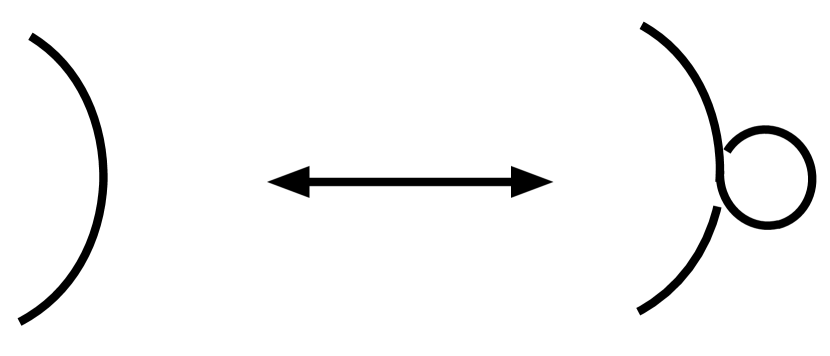
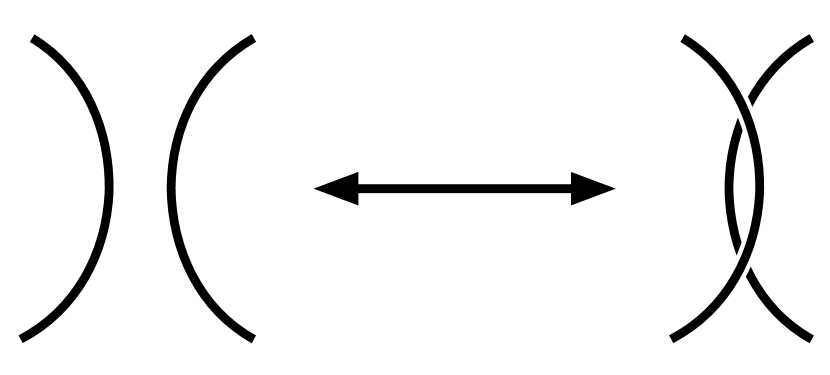

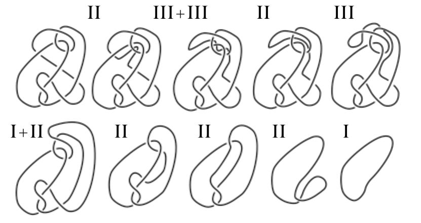
Farhi et al. instantiate their blueprint by picking to be the set of all links and the set of all polynomials.666666Here, we oversimplify the construction. In practice, they choose all links which are not too “large” according to their representation in a grid diagram. The function is the Alexander polynomial. This yields bill states of the following form:
| (69) |
The summation is taken over all links such that . Finally, note that is an exponentially large superposition over all links that have the same Alexander polynomial.
We may now use the knot invariance property of Alexander polynomials to perform verification. To see how this works, suppose is a unitary transformation that applies the Reidemeister move and note that for all and . The verification procedure effectively checks this invariance. This is done by adding an ancillary qubit in the state, applying a controlled- unitary, measuring the first qubit in the basis, and accepting if the outcome is . Note that , and therefore the verification will accept valid money. This is repeated many times with all 3 Reidemeister moves.676767Our presentation is intentionally simplistic and differs from the original presentation in Farhi et al. (2012). For example, the set of all links, , is infinite, and therefore one cannot generate the state in Equation (65). Farhi et al. (2012) also uses a specific representation of links called grid diagrams, along with grid moves, which are analogous to Reidemeister moves that can be efficiently applied to grid diagrams. This allows them to work with grid diagrams up to certain size, so that the set is finite.