Combining Reinforcement Learning with Lin-Kernighan-Helsgaun Algorithm
for the Traveling Salesman Problem

Jiongzhi Zheng ^1,2, Kun He¹, Jianrong Zhou¹, Yan Jin¹,Chu-Min Li ^1,3
Corresponding author.

Abstract

We address the Traveling Salesman Problem (TSP), a famous NP-hard combinatorial optimization problem. And we propose a variable strategy reinforced approach, denoted as VSR-LKH, which combines three reinforcement learning methods (Q-learning, Sarsa and Monte Carlo) with the well-known TSP algorithm, called Lin-Kernighan-Helsgaun (LKH). VSR-LKH replaces the inflexible traversal operation in LKH, and lets the program learn to make choice at each search step by reinforcement learning. Experimental results on 111 TSP benchmarks from the TSPLIB with up to 85,900 cities demonstrate the excellent performance of the proposed method.

Introduction

Given a set of cities with certain locations, the Traveling Salesman Problem (TSP) is to find the shortest route, along which a salesman travels from a city to visit all the cities exactly once and finally returns to the starting point. An algorithm designed for TSP can also be applied to many other practical problems, such as the Vehicle Routing Problem (VRP) (Nazari et al. 2018), tool path optimization of Computer Numerical Control (CNC) machining (Fok et al. 2019), etc. As one of the most famous NP-hard combinatorial optimization problems, TSP has become a touchstone for the algorithm design.

Numerous approaches have been proposed for solving the TSP. Traditional methods are mainly exact algorithms and heuristic algorithms, such as the exact solver Corconde ¹¹1http://www.math.uwaterloo.ca/tsp/concorde/index.html and the Lin-Kernighan-Helsgaun (LKH) heuristic (Helsgaun 2000; Helsgaun 2009; Taillard and Helsgaun 2019; Tinós, Helsgaun, and Whitley 2018). With the development of artificial intelligence, there are some studies combining reinforcement learning (Sutton and Barto 1998) with (meta) heuristics to solve the TSP (de O. da Costa et al. 2020; Liu and Zeng 2009), and attaining good results on instances with up to 2,400 cities. More recently, Deep Reinforcement Learning (DRL) methods (Khalil et al. 2017; Shoma, Daisuke, and Hiroyuki 2018; Xing, Tu, and Xu 2020; de O. da Costa et al. 2020) have also been used to solve the TSP. However, DRL methods are hard to scale to large instances with thousands of cities, indicating that current DRL methods still have a gap to the competitive heuristic algorithms.

Heuristic algorithms are currently the most efficient and effective approaches for solving the TSP, including real-world TSPs with millions of cities. The LKH algorithm (Helsgaun 2000), which improves the Lin-Kernighan (LK) heuristic (Lin and Kernighan 1973), is one of the most famous heuristics. LKH improves the route through the $k$ -opt heuristic optimization method (Lin 1965), which replaces at most $k$ edges of the current tour at each search step. The most critical part of LKH is to make choice at each search step. In the $k$ -opt process, it has to select edges to be removed and to be added. Differs to its predecessor LK heuristic of which each city has its own candidate set recording five (default value) nearest cities, LKH used an $\alpha$ -value defined based on the minimum spanning tree (Held and Karp 1970) as a metric in selecting and sorting cities in the candidate set. The effect of candidate sets greatly improves the iteration speed and the search speed of both LK and LKH.

However, when selecting edges to be added in the $k$ -opt process, LKH traverses the candidate set of the current city in ascending order of the $\alpha$ -value until the constraint conditions are met, which is inflexible and may limit its potential to find the optimal solution. In this work, we address the challenge of improving the LKH, and introduce a creative and distinctive method to combine reinforcement learning with the LKH heuristic. The proposed algorithm could learn to choose the appropriate edges to be added in the $k$ -opt process by means of a reinforcement learning strategy.

Concretely, we first use three reinforcement learning methods, namely Q-learning, Sarsa and Monte Carlo (Sutton and Barto 1998), to replace the inflexible traversal operation of LKH. The performance of the reinforced LKH algorithm by any one of the three methods has been greatly improved. Besides, we found that the three methods are complementary in reinforcing the LKH. For example, some TSP instances can be solved well by Q-learning, but not by Sarsa, and vice versa. Therefore, we propose a variable strategy reinforced approach, called VSR-LKH, that combines the above three algorithms to further improve the performance. The idea of variable strategy is inspired from Variable Neighborhood Search (VNS) (Mladenovic and Hansen 1997), which leverages the complementarity of different local search neighborhoods. The principal contributions are as follows:

•

We propose a reinforcement learning based heuristic algorithm called VSR-LKH that significantly promotes the well-known LKH algorithm, and demonstrate its promising performance on 111 public TSP benchmarks with up to 85,900 cities.
•

We define a Q-value to replace the $\alpha$ -value by combining the city distance and $\alpha$ -value for the selection and sorting of candidate cities. And Q-value can be adjusted adaptively by learning from the information of many feasible solutions generated during the iterative search.
•

Since algorithms solving an NP-hard combinatorial optimization problem usually need to make choice among many candidates at each search step, our approach suggests a way to improve conventional algorithms by letting them learn to make good choices intelligently.

Related Work

This section reviews related work in solving the TSP using exact algorithms, heuristic algorithms and reinforcement learning methods respectively.

Exact Algorithms.

The branch and bound (BnB) method is often used to exactly solve the TSP and its variants (Pekny and Miller 1990; Pesant et al. 1998). The best-known exact solver Corconde ¹ is based on BnB, whose initial tour is obtained by the Chained LK algorithm (Applegate, Cook, and Rohe 2003). Recently, the Corconde solver was sped up by improving the initial solution using a partition crossover (Sanches, Whitley, and Tinós 2017). All of these exact algorithms can yield optimal solutions, but the computational costs rise sharply along with the problem scale.

Heuristic Algorithms.

Although heuristic algorithms cannot guarantee the optimal solution, they can obtain a sub-optimal solution within reasonable time. Heuristic algorithms for solving the TSP can be divided into three categories: tour construction algorithms, tour improvement algorithms and composite algorithms.

Each step of the tour construction algorithms determines the next city the salesman will visit until the complete TSP tour is obtained. The nearest neighbor (NN) algorithm (Hougardy and Wilde 2015) and ant colony algorithm (Gao 2020) are among the most common methods for tour construction.

The tour improvement algorithms usually make improvements on a randomly initialized tour. The $k$ -opt algorithm (Lin 1965) and genetic algorithm fall into this category. The evolutionary algorithm represented by Nagata (2006) is one of the most successful genetic algorithms to solve TSP, which is based on an improved edge assembly crossover (EAX) operation. Its selection model can maintain the population diversity at low cost.

The composite algorithms usually use tour improvement algorithms to improve the initial solution obtained by a tour construction algorithm. The famous LKH algorithm is a composite algorithm that uses $k$ -opt to improve the heuristically constructed initial tour.

Reinforcement Learning based Methods.

With the rapid development of artificial intelligence, some researchers have adopted reinforcement learning technique for solving the TSP.

One category is to combine reinforcement learning or DRL with existing (meta) heuristics. Ant-Q (Gambardella and Dorigo 1995) and Q-ACS (Sun, Tatsumi, and Zhao 2001) replaced the pheromone in the ant colony algorithm with the Q-table in the Q-learning algorithm. However, the effect of Q-table is similar to that of the pheromone. Liu and Zeng (2009) used reinforcement learning to construct mutation individuals in the successful genetic algorithm EAX-GA (Nagata 2006) and reported results on instances with up to 2,400 cities, but their proposed algorithm RMGA is inefficient compared with EAX-GA and LKH. Costa et al. (2020) utilized DRL algorithm to learn a 2-opt based heuristic, Wu et al. (2019) combined DRL method with the tour improvement approach such as 2-opt and node swap. They reported results on real-world TSP instances with up to 300 cities.

Another category is to apply DRL to directly solve the TSP. Bello et al. (2017) addressed TSP by using the actor-critic method to train a pointer network (Vinyals, Fortunato, and Jaitly 2015). The S2V-DQN (Khalil et al. 2017) used reinforcement learning to train graph neural networks so as to solve several combinatorial optimization problems, including minimum vertex cover, maximum cut and TSP. Shoma et al. (2018) used reinforcement learning with a convolutional neural network to solve the TSP. The graph convolutional network technique (Joshi, Laurent, and Bresson 2019) was also applied to solve the TSP. The ECO-DQN (Barrett et al. 2020) is an improved version of S2V-DQN, which has obtained better results than S2V-DQN on the maximum cut problem. Xing et al. (2020) used deep neural network combined with Monte Carlo tree search to solve the TSP. It is generally hard for them to scale to large TSP instances with thousands cities as an effective heuristic such as LKH does.

In this work, we aim to combine reinforcement learning with existing excellent heuristic algorithm in a more effective way, and handle efficiently large scale instances. We reinforce the key component of LKH, the $k$ -opt, and thus promote the performance significantly. To our knowledge, this is the first work that combines reinforcement learning with the key search process of a well-known algorithm to solve the famous NP-hard TSP.

The Existing LKH Algorithm

We give a brief introduction to the LKH algorithm (see more details of LKH and its predecessor LK heuristic in Appendix). LKH uses $k$ -opt (Lin 1965) as the optimization method to improve the TSP tour. During the $k$ -opt process, LKH first selects a starting point $p_{1}$ , then alternately selects $k$ edges $\{x_{1},x_{2},...,x_{k}\}$ to be removed in the current tour and $k$ edges $\{y_{1},y_{2},...,y_{k}\}$ to be added until the stopping criterion is met ( $2\leq k\leq 5$ , which is not predetermined).

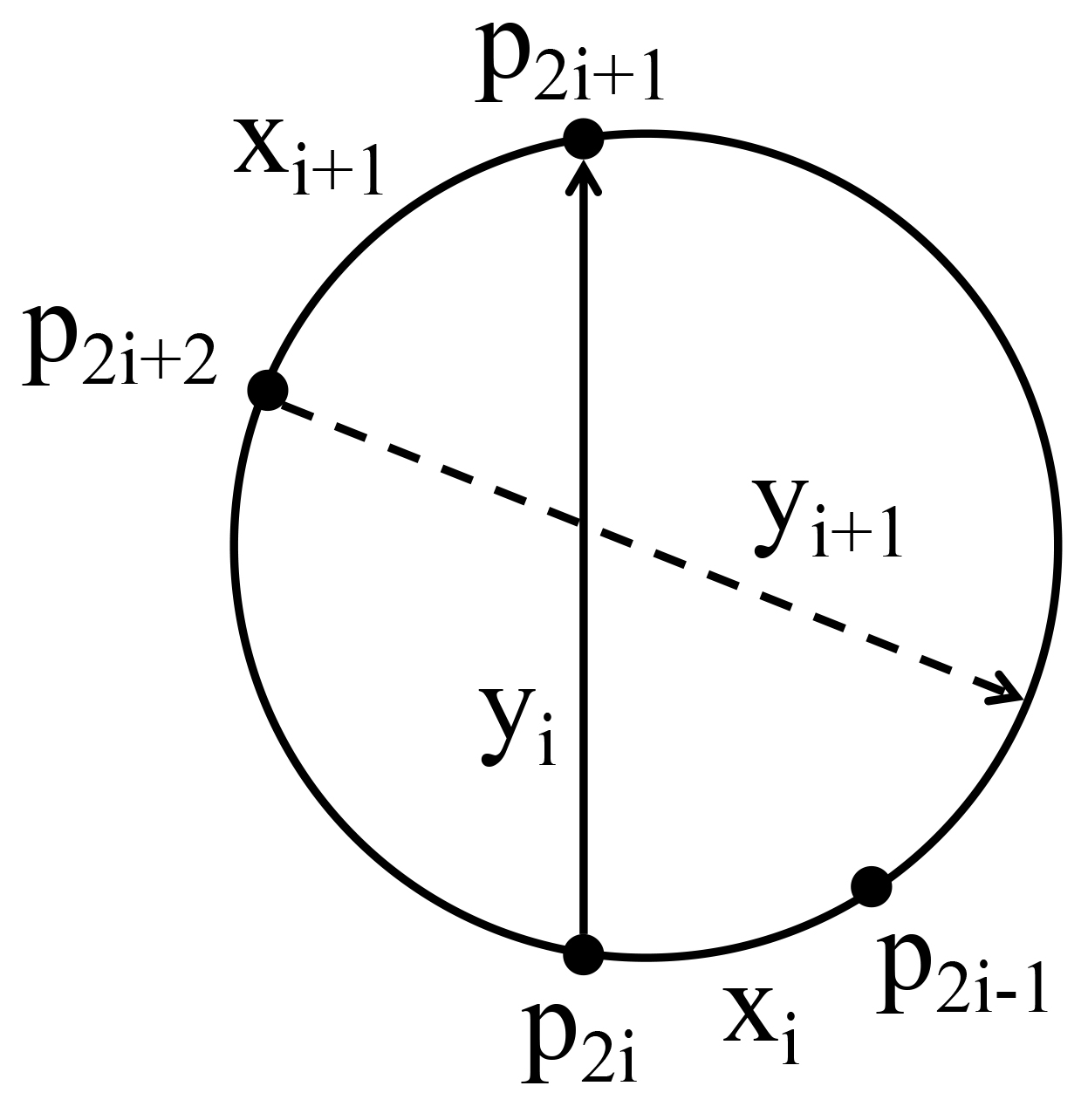
Refer to caption — Figure 1: The choice of $x_{i}$ , $y_{i}$ , $x_{i+1}$ and $y_{i+1}$ in $k$ -opt.

Figure 1 shows the iterative process of $k$ -opt in LKH. The key point is to select $2k$ cities $\{p_{1},p_{2},...,p_{2k}\}$ such that for each $i$ ( $1\leq i\leq k$ ), $x_{i}=(p_{2i-1},p_{2i})$ , for each $i$ ( $1\leq i\leq k-1$ ), $y_{i}=(p_{2i},p_{2i+1})$ and $y_{k}=(p_{2k},p_{1})$ . And the following conditions should be satisﬁed: (1) $x_{i}$ and $y_{i}$ must share an endpoint, and so do $y_{i}$ and $x_{i+1}$ ; (2) For $i\geq 2$ , if $p_{2i}$ connects back to $p_{1}$ for $y_{i}$ , the resulting configuration should be a tour; (3) $y_{i}$ is always chosen so that $\sum\nolimits_{j=1}^{i}(l(x_{j})-l(y_{j}))>0$ , where $l(\cdot)$ is the length of the corresponding edge; (4) Set { $x_{1},x_{2},...,x_{i}$ } and set { $y_{1},y_{2},...,y_{i}$ } are disjoint. To this end, LKH first randomly selects $p_{1}$ . After $p_{2i-1}$ is selected, $p_{2i}$ is randomly selected from the two neighbors of $p_{2i-1}$ in the current TSP tour. Then $p_{2i+1}$ is selected by traversing the candidate set of $p_{2i}$ .

The current iteration of $k$ -opt process will quit when a $k$ -opt move is found that can improve the current TSP tour (by trying to connect $p_{2k}$ with $p_{1}$ as $y_{k}$ before selecting $p_{2k+1}$ ) or no edge pair, $x_{i}$ and $y_{i}$ , satisfies the constraints.

The $\alpha$ -value.

The candidate set of each city in LKH stores five other cities in ascending order of the $\alpha$ -values. To explain $\alpha$ -value, we need to introduce the structure of 1-tree (Held and Karp 1970). A 1-tree for a graph $G(V,E)$ ( $V$ is the set of nodes, $E$ is the set of edges) is a spanning tree on the node set $V\backslash\{v\}$ combined with two edges from $E$ incident to node $v$ , which is a special point chosen arbitrarily. A minimum 1-tree is a 1-tree with minimum length.Obviously, the length of the minimum 1-tree is the lower bound of the optimal TSP solution. Suppose $L(T)$ is the length of the minimum 1-tree of graph $G(V,E)$ and $L(T^{+}(i,j))$ is the length of the minimum 1-tree required to contain edge $(i,j)$ , the $\alpha$ -value of edge $(i,j)$ can be calculated by Eq. 1:

\alpha(i,j)=L(T^{+}(i,j))-L(T).

(1)

Penalties.

LKH uses a method to maximize the lower bound of the optimal TSP solution by adding penalties (Held and Karp 1970). Concretely, a $\pi$ -value computed using a sub-gradient optimization method (Held and Karp 1971) is added to each node as a penalty when calculating the distance between two nodes:

C(i,j)=d(i,j)+\pi_{i}+\pi_{j},

(2)

where $C(i,j)$ is the cost for a salesman from city $i$ to city $j$ after adding penalties, $d(i,j)$ is the distance between the two cities, and $\pi_{i},\pi_{j}$ are the penalties added to the two cities respectively. The penalties actually change the cost matrix of the TSP. Note that this change does not change the optimal solution of the TSP, but it changes the minimum 1-tree. Suppose $L(T_{\pi})$ is the length of the minimum 1-tree after adding the penalties, then the lower bound $w(\pi)$ of the optimal solution can be calculated by Eq. 3, which is a function of set $\pi=[\pi_{1},...,\pi_{n}]$ :

w(\pi)=L(T_{\pi})-2\sum\limits_{i}\pi_{i}.

(3)

The lower bound $w(\pi)$ of the optimal solution is maximized, and after adding the penalties, the $\alpha$ -value is further improved for the candidate set.

The Proposed VSR-LKH Algorithm

The proposed Variable Strategy Reinforced LKH (VSR-LKH) algorithm combines reinforcement learning with LKH. In VSR-LKH, we change the method of traversing the candidate set in the $k$ -opt process and let the program automatically select appropriate edges to be added in the candidate set by reinforcement learning. We further use a variable strategy method that combines the advantages of three reinforcement learning methods, so that VSR-LKH can improve the flexibility as well as the robustness and avoid falling into local optimal solutions. We achieve VSR-LKH on top of LKH, so VSR-LKH still retains the characteristics of LKH such as candidate set, penalties and other improvements made by Helsgaun (Helsgaun 2009; Taillard and Helsgaun 2019; Tinós, Helsgaun, and Whitley 2018).

Reinforcement Learning Framework

Since VSR-LKH lets the program learn to make correct decisions for choosing the edges to be added, the states and actions in our reinforcement learning framework are all related to the edges to be added. And an episode corresponds to a $k$ -opt process. We use the value iteration method to estimate the state-action function $q_{\pi}(s,a)=\sum_{t=0}^{\infty}{\gamma^{t}{r(s_{t},a_{t})}}$ , where $(s_{t},a_{t})$ is the state-action pair at time step $t$ of an episode, $s_{0}=s,a_{0}=a$ , and $r$ is the corresponding reward. The detailed description of the states, actions and rewards in the reinforcement learning framework are as follows:

•

States: The current state of the system is a city that is going to select an edge to be added. For example in Figure 1, for edge $y_{i}$ , the state corresponds to its start point $p_{2i}$ . When $i=1$ , the initial state $s_{0}$ corresponds to $p_{2i}=p_{2}$ .
•

Actions: For a state $s$ , the action is to choose another endpoint of the edge to be added except $s$ from the candidate set of $s$ . For example in Figure 1, for edge $y_{i}$ , the action corresponds to its endpoint $p_{2i+1}$ . When $i=1$ , action $a_{0}$ corresponds to $p_{2i+1}=p_{3}$ .
•

Transition: The next state after performing the action is the next city that needs to select an edge to be added. For example, $p_{2i+2}$ is the state transferred to after executing action $p_{2i+1}$ at state $p_{2i}$ .

•

Rewards: The reward function should be able to represent the improvement of the tour when taking an action at the current state. The reward $r(s_{t},a_{t})$ obtained by performing action $a_{t}$ at state $s_{t}$ can be calculated by:

r(s_{t},a_{t})=\begin{cases}C(a_{t-1},s_{t})-C(s_{t},a_{t})&\text{$t>0$}\\ C(p_{1},s_{0})-C(s_{0},a_{0})&\text{$t=0$}\end{cases},

(4)

where function $C(\cdot,\cdot)$ is shown in Eq. 2.

Initial Estimation of the State-action Function

We associate the estimated value of the state-action function in VSR-LKH to each city and call it Q-value of the city. It is used as the basis for selecting and sorting the candidate cities. The initial Q-value $Q(i,j)$ for the candidate city $j$ of city $i$ is deﬁned as follows:

Q(i,j)=\frac{w(\pi)}{\alpha(i,j)+d(i,j)}.

(5)

The initial Q-value defined in Eq. 5 combines the factors of the selection and sorting of candidate cities in LK (Lin and Kernighan 1973) and LKH (Helsgaun 2000), which are the distance and the $\alpha$ -value, respectively. Note that $\alpha$ -value is based on a minimum 1-tree and is rather a global property, while the distance between two cities is a local property. Combining $\alpha$ -value and distance can take the advantage of both properties. The main factor dominating the initial Q-value is the $\alpha$ -value. Although the influence of the distance factor is small, it can avoid the denominator to be 0. The purpose of $w(\pi)$ is two-folds. First, it can prevent the initial Q-value from being much smaller than the rewards. Second, it can adaptively adjust the initial Q-value for different instances. The experimental results also demonstrate that the performance of LKH can be improved by only replacing $\alpha$ -value with the initial Q-value defined in Eq. 5 to select and sort the candidate cities.

The Reinforced Algorithms

VSR-LKH applies reinforcement technique to learn to adjust Q-value so as to estimate the state-action function more accurately. As the maximum value of $k$ in the $k$ -opt process of LKH is as small as 5, we choose the Monte Carlo method and one-step Temporal-Difference (TD) algorithms including Q-learning and Sarsa (Sutton and Barto 1998) to improve the $k$ -opt process in LKH.

Monte Carlo.

Monte Carlo method is well-known for the model-free reinforcement learning based on averaging sample returns. In the reinforcement learning framework, there was no repetitive state or action in one or even multiple episodes. Therefore, for any state action pair $(s_{t},a_{t})$ , the Monte Carlo method uses the episode return after taking action $a_{t}$ at state $s_{t}$ as the estimation of its Q-value. That is,

Q(s_{t},a_{t})=\sum\nolimits_{i=0}^{+\infty}{r(s_{t+i},a_{t+i})}.

(6)

One-step TD.

TD learning is a combination of Monte Carlo and Dynamic Programming. The TD algorithms can update the Q-values in an on-line, fully incremental fashion. In this work, we use both of the on-policy TD control (Sarsa) and off-policy TD control (Q-learning) to reinforce the LKH. The one-step Sarsa and Q-learning update the Q-value respectively as follows:

\begin{split}Q(s_{t},a_{t})=&(1-\lambda)\cdot{Q(s_{t},a_{t})}+\\ &\lambda\cdot[r(s_{t},a_{t})+\gamma{Q(s_{t+1},a_{t+1})}],\end{split}

(7)

\begin{split}Q(s_{t},a_{t})=&(1-\lambda)\cdot{Q(s_{t},a_{t})}+\\ &\lambda\cdot[r(s_{t},a_{t})+\gamma{\max\limits_{a^{\prime}}Q(s_{t+1},a^{\prime})}],\end{split}

(8)

where $\lambda\in(0,1)$ in Eq. 7 and Eq. 8 is the learning rate.

Variable Strategy Reinforced $k$ -opt

The VSR-LKH algorithm uses the reinforcement learning technique to estimate the state-action function to determine the optimal policy. The policy guides the program to select the appropriate edges to be added in the $k$ -opt process. Moreover, a variable strategy method is added to combine the advantages of the three reinforcement learning algorithms, Q-learning, Sarsa and Monte Carlo, and leverages their complementarity. When VSR-LKH judges that the current reinforcement learning method (Q-learning, Sarsa or Monte Carlo) may not be able to continue optimizing the current TSP tour, the variable strategy mechanism will switch to another method. Algorithm 1 shows the flow of the variable strategy reinforced $k$ -opt process of VSR-LKH. And the source code of VSR-LKH is available at https://github.com/JHL-HUST/VSR-LKH/.

Algorithm 1 Variable strategy reinforced

k

-opt process

\epsilon

-greedy parameter:

\epsilon

, attenuation coefficient:

\beta

, BestTour=ChooseInitialTour(), maximum number of iterations: MaxTrials, variable strategy parameters: MaxNum

0: BestTour

Initialize Q-values according to Eq. 5

CreateCandidateSet()

Initialize

M=1

that corresponds to the policy (1: Q-learning, 2: Sarsa, 3: Monte Carlo), initialize

num=0

for

i=1:MaxTrials

num=num+1

\epsilon=\epsilon\times{\beta}

num\geq{MaxNum}

then

M=M\%{3}+1,num=0

end if

BetterTour=ChooseInitialTour()

repeat

Randomly select an unselected edge

(p_{1},p_{2})

in BetterTour as the initial edge

Initialize the set of edges to be removed

\mathcal{R}_{e}=\emptyset

, the set of edges to be added

\mathcal{A}_{e}=\emptyset

\mathcal{R}_{e}:=\mathcal{R}_{e}\cup\{(p_{1},p_{2})\}

, set

k=1

Suppose

C_{2k}

is the candidate set of

p_{2k}

while the stopping criterion is not satisfied do

p_{2k+1}=\epsilon

greedy(C_{2k})

C_{2k}:=C_{2k}\backslash\{p_{2k+1}\}

p_{2k+1}

does not satisfy the constraints then

continue

end if

Randomly traverse the two neighbors of

p_{2k+1}

to select

p_{2k+2}

that satisfies the constraints

Update

Q(p_{2k},p_{2k+1})

according to Eq. 6, 7 or 8 corresponding to

M

\mathcal{A}_{e}:=\mathcal{A}_{e}\cup\{(p_{2k},p_{2k+1})\}

\mathcal{R}_{e}:=\mathcal{R}_{e}\cup\{(p_{2k+1},p_{2k+2})\}

k=k+1

end while

\mathcal{A}_{e}:=\mathcal{A}_{e}\cup\{(p_{2k},p_{1})\}

if the sum of lengths of all edges in

\mathcal{A}_{e}

is less than that in

\mathcal{R}_{e}

then

Replace edges in

\mathcal{R}_{e}

with edges in

\mathcal{A}_{e}

and set the new tour as BetterTour

break

end if

until each edge in BetterTour has been selected as the initial edge (Note that edges

(i,j)

and

(j,i)

are different)

if length of BetterTour is less than BestTour then

Replace BestTour with BetterTour,

num=0

end if

Exit if BestTour is equal to the optimum (if known)

end for

In Algorithm 1, we apply two functions ChooseInitialTour() and CreateCandidateSet() in LKH to initialize the initial tour of TSP and the candidate sets of all cities. VSR-LKH uses the $\epsilon$ -greedy method (Sutton and Barto 1998; Wunder, Littman, and Babes 2010) to trade-off the exploration-exploitation dilemma in the reinforcement learning process. And the value of $\epsilon$ is reduced by the attenuation coefficient $\beta$ to make the algorithm inclined to exploitation as the number of iterations increases. The reinforcement learning strategy is switched if the algorithm could not improve the solution after a certain number of iterations, denoted as MaxNum. Each iteration in the $k$ -opt process of VSR-LKH needs to find cities $p_{2k+1}$ and $p_{2k+2}$ that meet the constraints before updating the Q-value. The final TSP route is stored in BestTour.

Experimental Results

Experimental results provide insight on why and how the proposed approach is effective, suggesting that the performance of VSR-LKH is due to the flexibility and robustness of variable strategy reinforced learning and the benefit of our Q-value definition that combines city distance and $\alpha$ -value.

Experimental Setup

The experiments were performed on a personal computer with Intel® i5-4590 3.30 GHz 4-core CPU and 8 GB RAM. The parameters related to reinforcement learning in VSR-LKH are set as follows: $\epsilon=0.4$ , $\beta=0.99$ , $\lambda=0.1$ , $\gamma=0.9$ , the maximum iterations, MaxTrials is equal to the number of cities in the TSP, and $MaxNum=MaxTrials/20$ . Actually, VSR-LKH is not very sensitive to these parameters. The performance of VSR-LKH with different parameters is compared in Appendix. Other parameters are consistent with the example given in the LKH open source website ²²2http://akira.ruc.dk/%7Ekeld/research/LKH/, and the LKH baseline used in our experiments is also from this website.

All the TSP instances are from the TSPLIB ³³3http://comopt.ifi.uni-heidelberg.de/software/TSPLIB95/, including 111 symmetric TSPs. Among them, there are 77 instances with less than 1,000 cities and 34 instances with at least 1,000 cities. The number of cities in these instances ranges from 14 to 85,900. Each instance is solved 10 times by each tested algorithm. An instance is considered to be easy if both LKH and VSR-LKH can reach the optimal solution in each of the 10 runs (for each run, the maximum number of iterations MaxTrials equals to the number of cities), and otherwise it is considered to be hard. All hard instances with less than 1,000 cities include: kroB150, si175, rat195, gr229, pr299, gr431, d493, att532, si535, rat575 and gr666, a total of 11. All instances with at least 1,000 cities in TSPLIB except dsj1000, si1032, d1291, u1432, d1655, u2319, pr2392 and pla7397 are hard, a total of 26. So there are 37 hard instances and 74 easy instances in TSPLIB. Note that the number in an instance name indicates the number of cities in that instance.

We tested VSR-LKH on all the 111 symmetric TSP instances from the TSPLIB, but mainly use results on the hard instances to compare different algorithms for clarity.

Q-value Evaluation

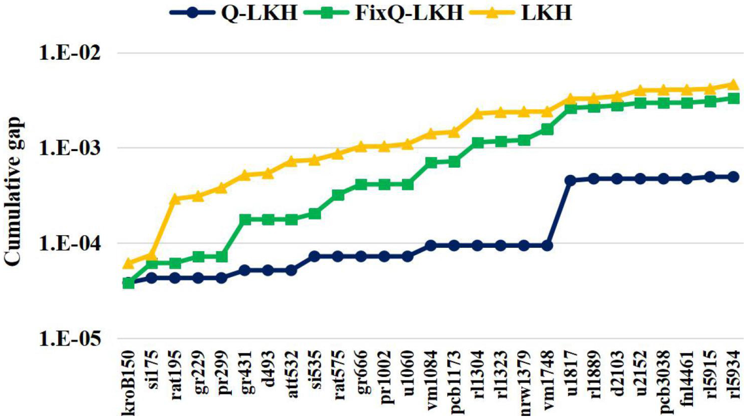
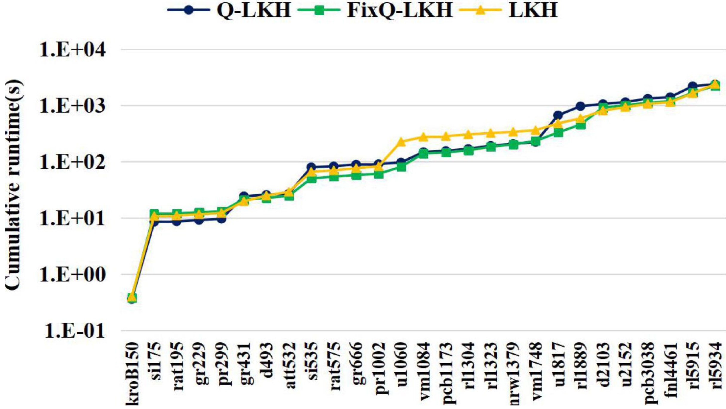
In order to demonstrate the positive influence of the Q-value we proposed in Eq. 5 on the performance, we pick 27 hard instances having the shortest runtime by LKH, and compare the results of three algorithms, including LKH, Q-LKH (a variant of VSR-LKH reinforced only by Q-learning, i.e. $M$ is always 1 in Algorithm 1) and FixQ-LKH (a variant of VSR-LKH with fixed Q-value defined by Eq. 5 and without reinforcement learning). FixQ-LKH is equivalent to LKH but uses the initial Q-value defined by Eq. 5 instead of $\alpha$ -value to select and sort the candidate cities.

Figure 2 shows the comparison results on TSP instances. Each instance is solved 10 times by the above three algorithms. The results are expressed by the cumulative gap on solution quality and cumulative runtime, because cumulants are more intuitive than comparing the results of each instance individually. $gap(a,j)=\frac{1}{10}\sum_{i=1}^{10}\frac{A_{i}-Opt_{j}}{Opt_{j}}$ is the average gap of calculating the $j$ -th instance by algorithm $a$ , where $A_{i}$ is the result of the $i$ -th calculation and $Opt_{j}$ is the optimal solution of the $j$ -th instance. The smaller the average gap, the closer the average solution is to the optimal solution. $C_{gap}(a,j)=\sum_{i=1}^{j}gap(a,i)$ is the cumulative gap. The cumulative runtime is calculated analogously.

As shown in Figure 2(a), the solution quality of LKH is lower than that of FixQ-LKH, indicating that LKH can be improved by only replacing $\alpha$ -value with Q-value defined in Eq. 5 to select and sort candidate cities. The results of Q-LKH compared with FixQ-LKH in Figure 2(a) demonstrate the positive effects of reinforcement learning method (Q-learning) that learns to adjust Q-value during the iterations. In addition, as shown in Figure 2(b), there is almost no difference in efficiency among the three algorithms when solving the 27 hard instances.

Comparison on Reinforcement Strategies

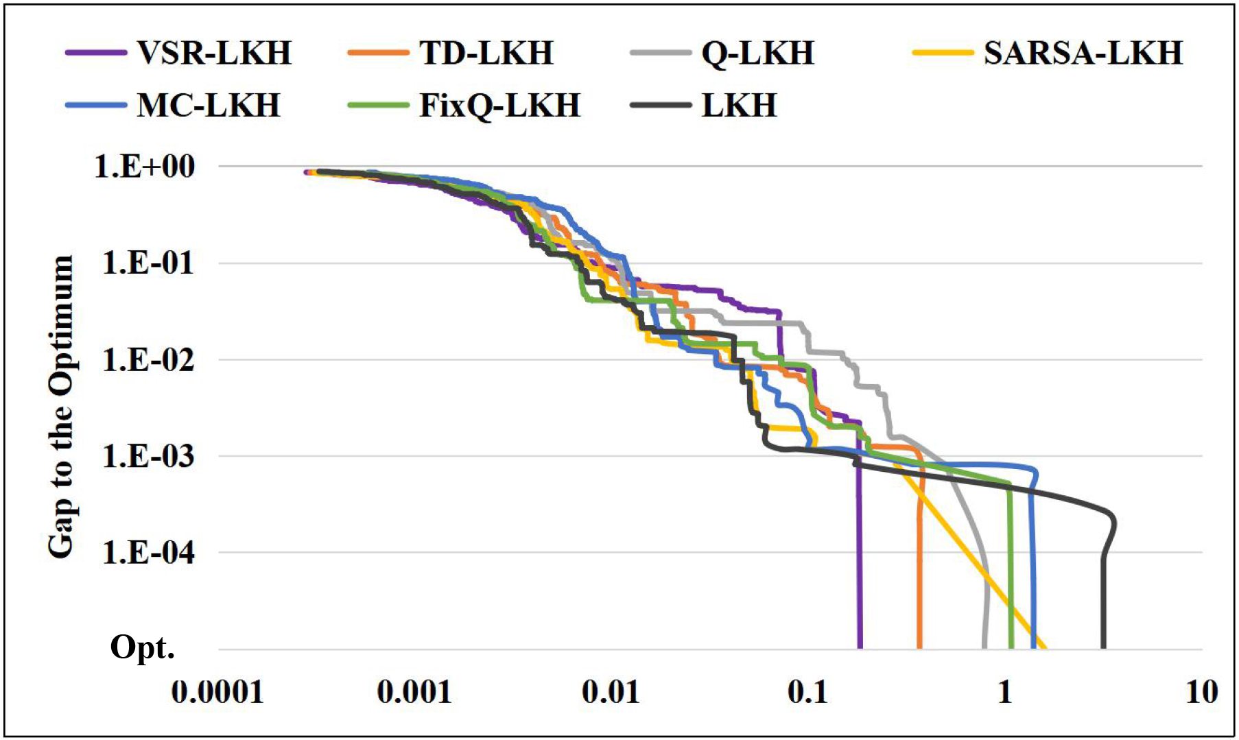
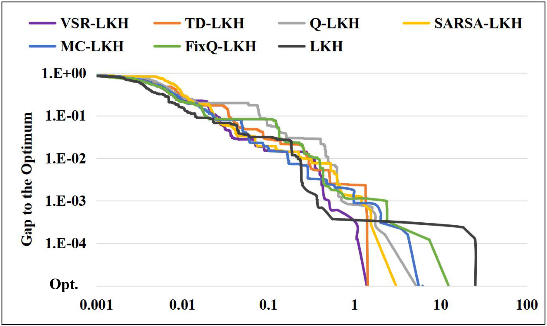
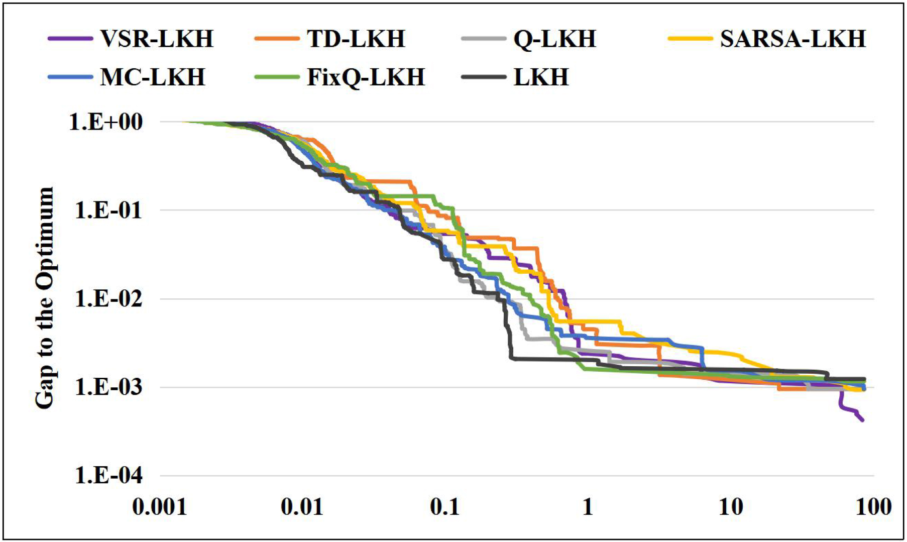
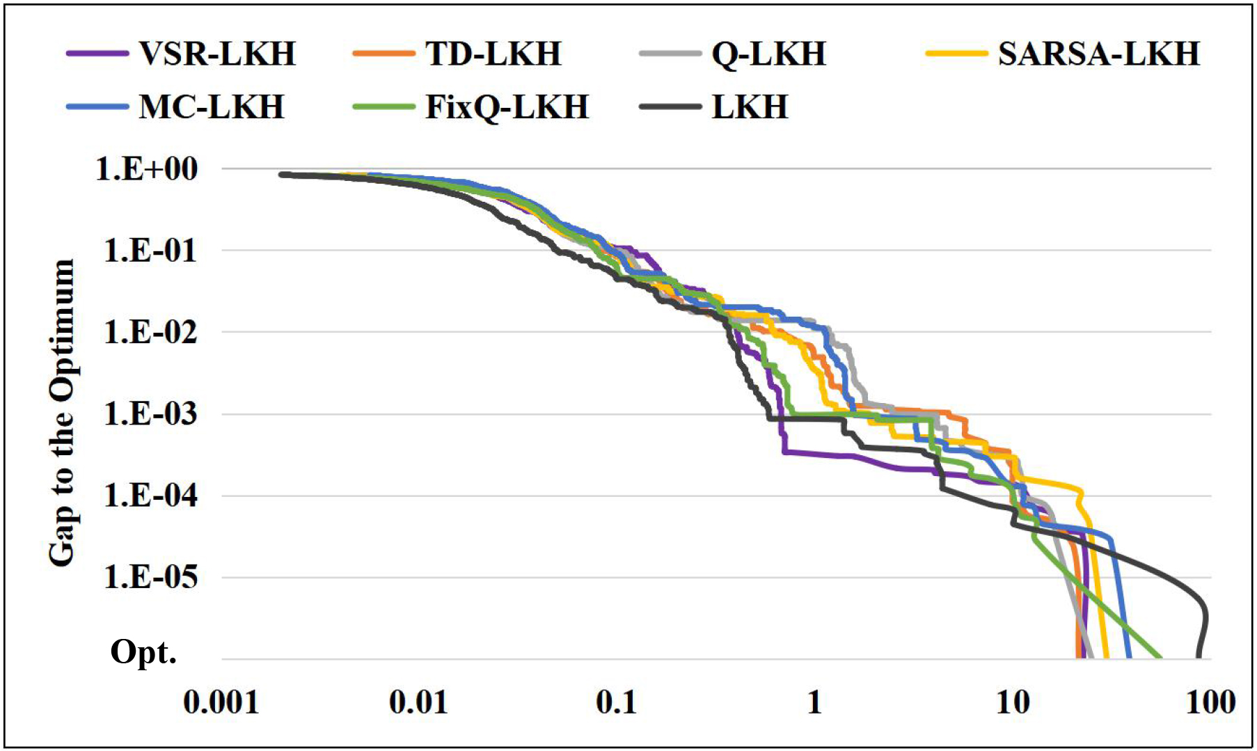
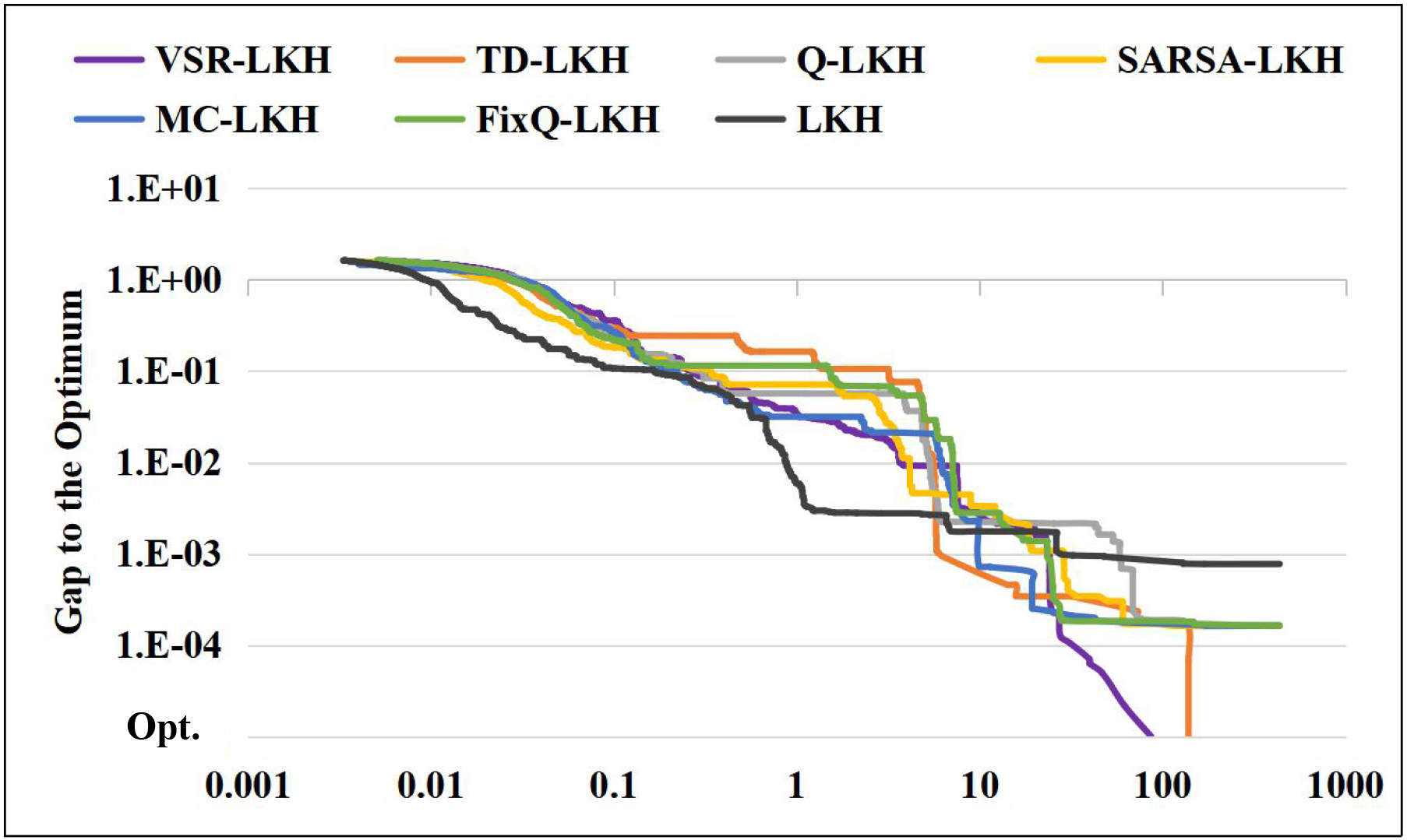
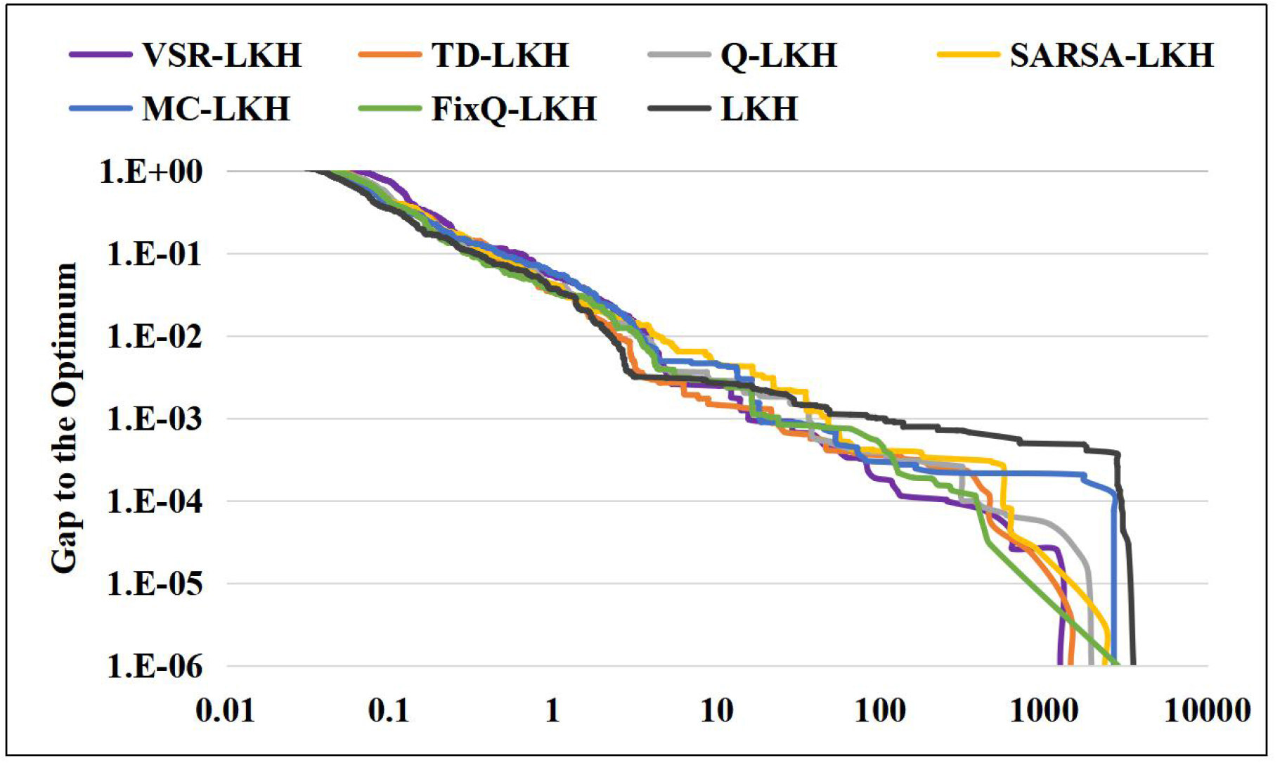
Here we compare the effectiveness of the three reinforcement learning strategies (Q-learning, Sarsa and Monte Carlo) in reinforcing the LKH. The three variants of VSR-LKH reinforced only by Q-learning, Sarsa or Monte Carlo are called Q-LKH, SARSA-LKH and MC-LKH ( $M$ is fixed to be always 1, 2, or 3 in Algorithm 1 to obtain these three variants, respectively). Figure 3 shows their results coupled with the results of LKH, VSR-LKH and TD-LKH (a variant of VSR-LKH reinforced by Q-learning and Sarsa, $M$ being 1 and 2 in turn in Algorithm 1) in solving the same set of 27 hard instances in Figure 2. Each instance in Figure 3 is also calculated 10 times to get the average results.

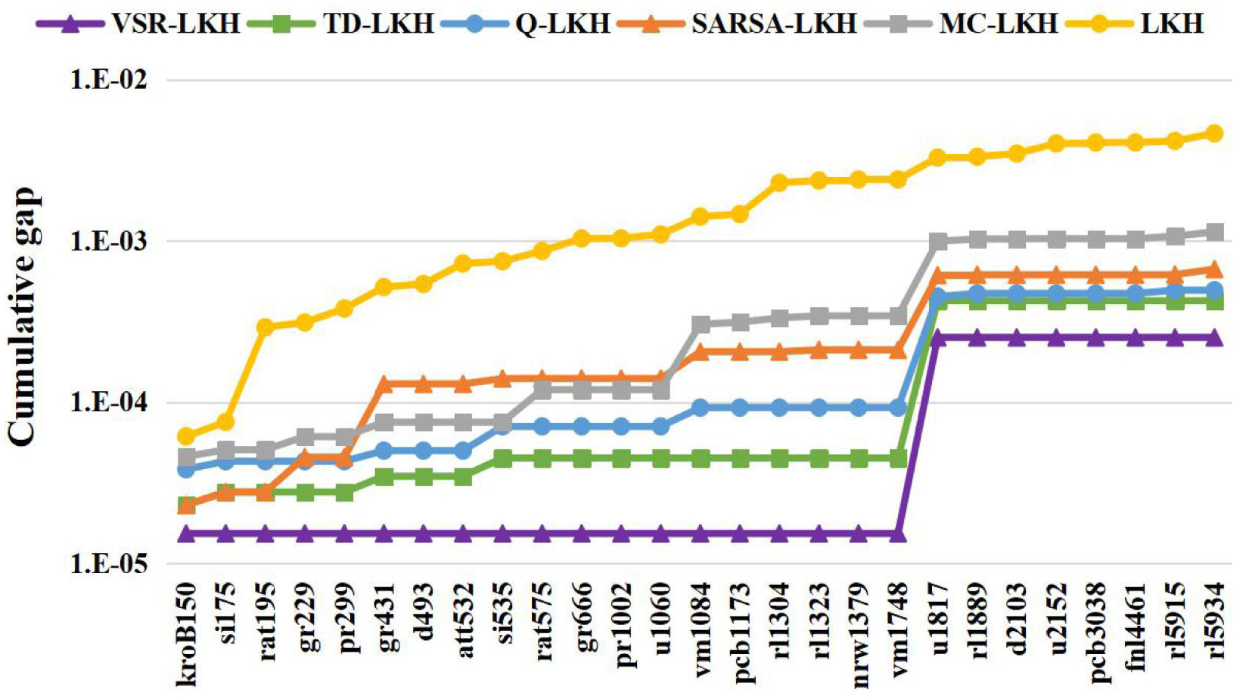
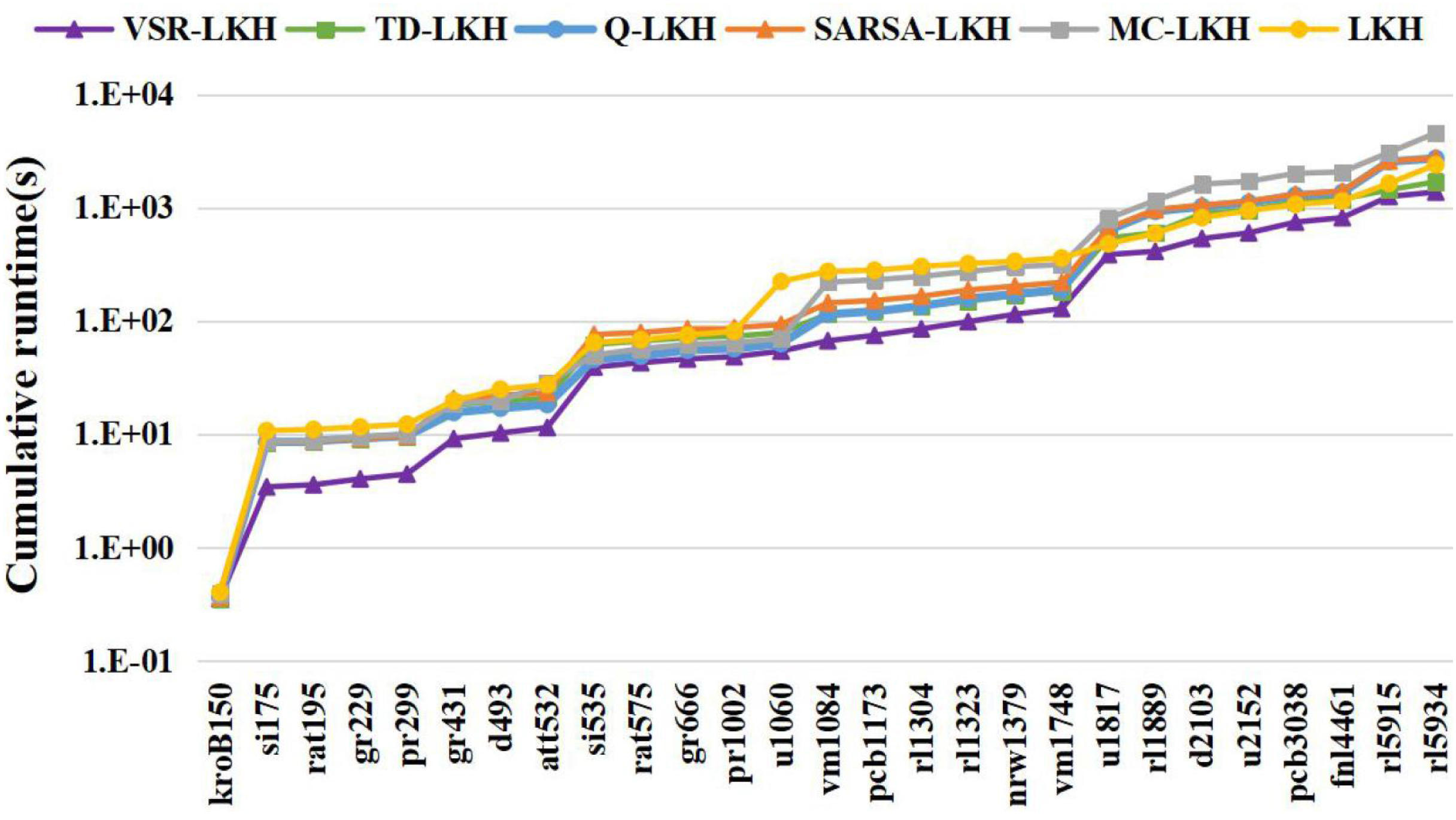
As shown in Figure 3, incorporating any one of the three reinforcement learning methods (Q-learning, Sarsa or Monte Carlo) to the LKH can greatly improve the performance. And the three strategies are complementary in reinforcing LKH. For example, Q-LKH has better results than SARSA-LKH or MC-LKH in most instances in Figure 3(a), but in solving some instances like kroB150, si535 and rl5915, Q-LKH is not as good as SARSA-LKH.

Therefore, we proposed VSR-LKH to combine the advantages of the three reinforcement methods and leverage their complementarity. Since Q-learning has the best performance in reinforcing LKH, we order Q-learning first and then Sarsa. Monte Carlo is ordered in the last since it is not good at solving large scale TSP. The order of Q-learning and Sarsa in TD-LKH is the same as in VSR-LKH.

As shown in Figure 3, TD-LKH and VSR-LKH further improve the solution quality compared with the three reinforced LKHs with a single method, and the two composite reinforced LKHs are significantly better than the original LKH. In addition, though the results of MC-LKH in Figure 3(a) are the worst among single reinforcement algorithms when solving large scale TSP instances, the TD-LKH without Monte Carlo is not as efficient as VSR-LKH and is not as good as VSR-LKH in solving the instances such as gr431, si535 and u1817. Thus, adding the Monte Carlo method in VSR-LKH is effective and necessary.

Moreover, we randomly selected six instances (u574, u1060, u1817, fnl4461, rl5934 and rl11849) to compare the calculation results over the runtime of LKH and various variants of VSR-LKH. See detailed results in Appendix.

NAME	Opt.	VSR-LKH	S2V-DQN	Xing et al.
eil51	426	Opt.	439	442
berlin52	7542	Opt.	Opt.	7598
st70	675	Opt.	696	695
eil76	538	Opt.	564	545
pr76	108159	Opt.	108446	108576

Table 1: Comparison of VSR-LKH and DRL algorithms on five easy instances (best results in bold).

NAME	Opt.	Method	Best	Average	Worst	Success	Time(s)	Trials
kroB150	26130	LKH	Opt.	26131.6	26132	2/10	0.40	128.4
kroB150	26130	VSR-LKH	Opt.	26130.4	26132	8/10	0.35	61.5
d493	35002	LKH	Opt.	35002.8	35004	6/10	5.24	219.6
d493	35002	VSR-LKH	Opt.	Opt.	Opt.	10/10	1.14	10.2
u1060	224094	LKH	Opt.	224107.5	224121	5/10	142.07	663.3
u1060	224094	VSR-LKH	Opt.	Opt.	Opt.	10/10	5.68	13.7
u1817	57201	LKH	Opt.	57251.1	57274	1/10	116.39	1817.0
u1817	57201	VSR-LKH	Opt.	57214.5	57254	7/10	256.79	766.9
rl1889	316536	LKH	316549	316549.8	316553	0/10	109.78	1889.0
rl1889	316536	VSR-LKH	Opt.	Opt.	Opt.	10/10	26.30	91.9
d2103	80450	LKH	80454	80462.0	80473	0/10	216.48	2103.0
d2103	80450	VSR-LKH	Opt.	Opt.	Opt.	10/10	121.97	511.8
rl5915	565530	LKH	565544	565581.2	565593	0/10	494.81	5915.0
rl5915	565530	VSR-LKH	Opt.	Opt.	Opt.	10/10	438.50	851.4
rl5934	556045	LKH	556136	556309.8	556547	0/10	753.22	5934.0
rl5934	556045	VSR-LKH	Opt.	Opt.	Opt.	10/10	118.78	144.6
rl11849	923288	LKH	Opt.	923362.7	923532	2/10	3719.35	10933.4
rl11849	923288	VSR-LKH	Opt.	Opt.	Opt.	10/10	1001.11	751.9
usa13509	19982859	LKH	Opt.	19983103.4	19983569	1/10	4963.52	13509.0
usa13509	19982859	VSR-LKH	Opt.	19982930.2	19983029	5/10	25147.63	11900.0

Table 2: Comparison of VSR-LKH and LKH on some hard instances, best results in bold (see full results in Appendix).

Final Comparison

We compare VSR-LKH with recent Deep Reinforcement Learning (DRL) algorithms for solving TSP, including S2V-DQN (Khalil et al. 2017) and Xing et al.’s method (2020). Table 1 compares VSR-LKH and the DRL algorithms in solving five easy instances with fewer than 100 cities that Xing et al. picked (Xing et al. only addressed instances with fewer than 100 cities). Column Opt. indicates the optimal solution of the corresponding instance. Each result of VSR-LKH is the average solution of 10 runs. Table 1 shows that VSR-LKH can always yield the optimal solution and is significantly better than the DRL algorithms.

Note that DRL algorithms are hard to scale to large scale problems. S2V-DQN provided results on 38 TSPLIB instances with the number of cities ranges from 51 to 318, but it didn’t tackle larger instances due to the limitation of memory on a single graphics card. And the gap between the results of S2V-DQN and the optimal solution becomes larger when solving TSPs with more than 100 cities.

We then compare VSR-LKH and LKH on all the 111 TSPLIB instances. Table 2 shows detailed comparison on several typical hard instances with various scales (see full results on all easy and hard instances in Appendix). The two methods both run 10 times for each TSP instance in Table 2, and we compare the best solution, the average solution and the worst solution. Column Success indicates the number of times the algorithm obtains optimal solution, Time is the average calculation time of the algorithm and Trials is the average number of iterations of VSR-LKH and LKH.

As shown in Table 2, VSR-LKH outperforms LKH on every instance, especially on four hard instances, rl1889, d2103, rl5915 and rl5934, that LKH did not yield optimal solution. Note that VSR-LKH also achieves good results in solving large scale TSP instances with more than 10,000 cities (rl11849 and usa13509). Actually, VSR-LKH can yield optimal solution on almost all the 111 instances (a total of 107, except fl1577, d18512, pla33810 and pla85900) in 10 runs. And the average solution of VSR-LKH is also Opt. on most of the 111 instances (a total of 102, except kroB150, fl1577, u1817, usa13509, brd14051, d15112, d18512, pla33810, pla85900), indicating that VSR-LKH can always obtain optimal solution on these instances in 10 runs.

For the two super large instances, pla33810 and pla85900, we limit the maximum single runtime of LKH and VSR-LKH to 100,000 seconds due to the resource limit. And VSR-LKH can yield better results than LKH with the same runtime when solving these two instances (see Appendix).

In terms of efficiency, when solving the 111 TSPLIB instances, the average number of iterations of VSR-LKH is no more than that of LKH on 100 instances, especially for some hard instances (1060, rl1889, rl5934 and rl11849). Although VSR-LKH takes longer time than LKH in a single iteration because it needs to trade-off the exploration and exploitation in the reinforcement learning process, it can find the optimal solution with fewer Trials than LKH and terminate the iteration in advance. So the average runtime of VSR-LKH is less than that of LKH on most instances. In general, the proposed variable strategy reinforcement learning method greatly improves the performance of the LKH algorithm.

Conclusion

We combine reinforcement learning technique with typical heuristic search method, and propose a variable strategy reinforced method called VSR-LKH for the NP-hard traveling salesman problem (TSP). We define a Q-value as the metric for the selection and sorting of candidate cities, and change the method of traversing candidate set in selecting the edges to be added, and let the program learn to select appropriate edges to be added in the candidate set through reinforcement learning. VSR-LKH combines the advantages of three reinforcement methods, Q-learning, Sarsa and Monte Carlo, and further improves the flexibility and robustness of the proposed algorithm. Extensive experiments on public benchmarks show that VSR-LKH outperforms signiﬁcantly the famous heuristic algorithm LKH.

VSR-LKH is essentially a reinforcement on the $k$ -opt process of LKH. Thus, other algorithms based on $k$ -opt could also be strengthened by our method. Furthermore, our work demonstrates the feasibility and privilege of incorporating reinforcement techniques with heuristics in solving classic combinatorial optimization problems. In future work, we plan to apply our approach in solving the constrained TSP and the vehicle routing problem.

Acknowledgments

This work is supported by National Natural Science Foundation (62076105).

References

Applegate, Cook, and Rohe (2003) Applegate, D. L.; Cook, W. J.; and Rohe, A. 2003. Chained Lin-Kernighan for Large Traveling Salesman Problems. INFORMS Journal on Computing 15(1): 82–92.
Barrett et al. (2020) Barrett, T. D.; Clements, W. R.; Foerster, J. N.; and Lvovsky, A. 2020. Exploratory Combinatorial Optimization with Reinforcement Learning. In AAAI, 3243–3250.
Bello et al. (2017) Bello, I.; Pham, H.; Le, Q. V.; Norouzi, M.; and Bengio, S. 2017. Neural Combinatorial Optimization with Reinforcement Learning. In ICLR.
de O. da Costa et al. (2020) de O. da Costa, P. R.; Rhuggenaath, J.; Zhang, Y.; and Akcay, A. 2020. Learning 2-opt Heuristics for the Traveling Salesman Problem via Deep Reinforcement Learning. CoRR abs/2004.01608.
Fok et al. (2019) Fok, K.; Cheng, C.; Ganganath, N.; Iu, H. H.; and Tse, C. K. 2019. An ACO-Based Tool-Path Optimizer for 3-D Printing Applications. IEEE Transactions on Industrial Informatics 15(4): 2277–2287.
Gambardella and Dorigo (1995) Gambardella, L. M.; and Dorigo, M. 1995. Ant-Q: A Reinforcement Learning Approach to the Traveling Salesman Problem. In ICML, 252–260.
Gao (2020) Gao, W. 2020. New Ant Colony Optimization Algorithm for the Traveling Salesman Problem. International Journal of Computational Intelligence Systems 13(1): 44–55.
Held and Karp (1970) Held, M.; and Karp, R. M. 1970. The Traveling-Salesman Problem and Minimum Spanning Trees. Operations Research 18(6): 1138–1162.
Held and Karp (1971) Held, M.; and Karp, R. M. 1971. The traveling-salesman problem and minimum spanning trees: Part II. Mathematical Programming 1(1): 6–25.
Helsgaun (2000) Helsgaun, K. 2000. An effective implementation of the Lin-Kernighan traveling salesman heuristic. European Journal of Operational Research 126(1): 106–130.
Helsgaun (2009) Helsgaun, K. 2009. General k-opt submoves for the Lin-Kernighan TSP heuristic. Mathematical Programming Computation 1(2-3): 119–163.
Hougardy and Wilde (2015) Hougardy, S.; and Wilde, M. 2015. On the nearest neighbor rule for the metric traveling salesman problem. Discrete Applied Mathematics 195: 101–103.
Joshi, Laurent, and Bresson (2019) Joshi, C. K.; Laurent, T.; and Bresson, X. 2019. An Efficient Graph Convolutional Network Technique for the Travelling Salesman Problem. CoRR abs/1906.01227.
Khalil et al. (2017) Khalil, E. B.; Dai, H.; Zhang, Y.; Dilkina, B.; and Song, L. 2017. Learning Combinatorial Optimization Algorithms over Graphs. In NIPS, 6348–6358.
Lin (1965) Lin, S. 1965. Computer solutions of the traveling salesman problem. Bell Labs Technical Journal 44(10): 2245–2269.
Lin and Kernighan (1973) Lin, S.; and Kernighan, B. W. 1973. An Effective Heuristic Algorithm for the Traveling-Salesman Problem. Operations Research 21(2): 498–516.
Liu and Zeng (2009) Liu, F.; and Zeng, G. 2009. Study of genetic algorithm with reinforcement learning to solve the TSP. Expert Systems with Applications 36(3): 6995–7001.
Mladenovic and Hansen (1997) Mladenovic, N.; and Hansen, P. 1997. Variable neighborhood search. Computers & Operations Research 24(11): 1097–1100.
Nagata (2006) Nagata, Y. 2006. Fast EAX Algorithm Considering Population Diversity for Traveling Salesman Problems. In EvoCOP, volume 3906, 171–182.
Nazari et al. (2018) Nazari, M.; Oroojlooy, A.; Snyder, L. V.; and Takác, M. 2018. Reinforcement Learning for Solving the Vehicle Routing Problem. In NeurIPS, 9861–9871.
Pekny and Miller (1990) Pekny, J. F.; and Miller, D. L. 1990. An Exact Parallel Algorithm for the Resource Constrained Traveling Salesman Problem with Application to Scheduling with an Aggregate Deadline. In ACM Conference on Computer Science, 208–214.
Pesant et al. (1998) Pesant, G.; Gendreau, M.; Potvin, J.; and Rousseau, J. 1998. An Exact Constraint Logic Programming Algorithm for the Traveling Salesman Problem with Time Windows. Transportation Science 32(1): 12–29.
Sanches, Whitley, and Tinós (2017) Sanches, D. S.; Whitley, L. D.; and Tinós, R. 2017. Improving an exact solver for the traveling salesman problem using partition crossover. In GECCO, 337–344.
Shoma, Daisuke, and Hiroyuki (2018) Shoma, M.; Daisuke, Y.; and Hiroyuki, E. 2018. Applying Deep Learning and Reinforcement Learning to Traveling Salesman Problem. In ICCECE.
Sun, Tatsumi, and Zhao (2001) Sun, R.; Tatsumi, S.; and Zhao, G. 2001. Multiagent reinforcement learning method with an improved ant colony system. In SMC, 1612–1617.
Sutton and Barto (1998) Sutton, R. S.; and Barto, A. G. 1998. Reinforcement learning - an introduction. Adaptive computation and machine learning. MIT Press.
Taillard and Helsgaun (2019) Taillard, É. D.; and Helsgaun, K. 2019. POPMUSIC for the travelling salesman problem. European Journal of Operational Research 272(2): 420–429.
Tinós, Helsgaun, and Whitley (2018) Tinós, R.; Helsgaun, K.; and Whitley, L. D. 2018. Efficient Recombination in the Lin-Kernighan-Helsgaun Traveling Salesman Heuristic. In PPSN XV, volume 11101, 95–107.
Vinyals, Fortunato, and Jaitly (2015) Vinyals, O.; Fortunato, M.; and Jaitly, N. 2015. Pointer Networks. In NIPS, 2692–2700.
Wu et al. (2019) Wu, Y.; Song, W.; Cao, Z.; Zhang, J.; and Lim, A. 2019. Learning improvement heuristics for solving the travelling salesman problem. arXiv preprint arXiv:1912.05784 .
Wunder, Littman, and Babes (2010) Wunder, M.; Littman, M. L.; and Babes, M. 2010. Classes of Multiagent Q-learning Dynamics with epsilon-greedy Exploration. In ICML, 1167–1174.
Xing, Tu, and Xu (2020) Xing, Z.; Tu, S.; and Xu, L. 2020. Solve Traveling Salesman Problem by Monte Carlo Tree Search and Deep Neural Network. CoRR abs/2005.06879.

Appendix

In the Appendix, we provide detailed description of the existing LKH algorithms, and more experimental results.

The Existing LKH Algorithms

In this section, we first introduce the Lin-Kernighan (LK) heuristic (Lin and Kernighan 1973), which is the predecessor algorithm of LKH, then explain the main improvements of LKH over LK.

The Lin-Kernighan Algorithm

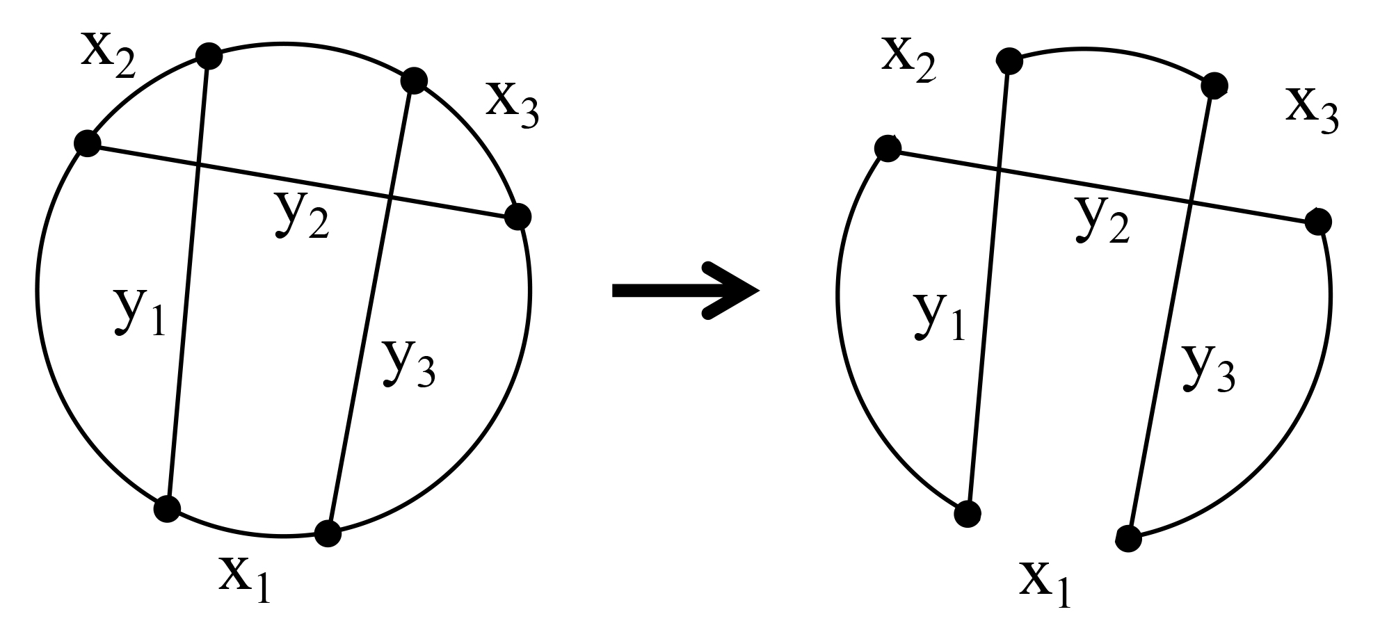
LK heuristic uses $k$ -opt (Lin 1965) as the optimization method to find optimal or sub-optimal solutions. Figure 4 illustrates a 3-opt move. The 3-opt process runs iteratively. At each iteration it attempts to change the tour by cutting three edges $x_{1}$ , $x_{2}$ , $x_{3}$ and replacing with three edges $y_{1}$ , $y_{2}$ , $y_{3}$ , then picks a better tour from the two. The key point of $k$ -opt is how to select these $x_{i}$ and $y_{i}$ , $i\in\{1,2,...,k\}$ , aka the edges to be removed in current TSP tour and the edges to be added.

The LK algorithm has two main contributions. Firstly, LK relieves the limitation that traditional $k$ -opt algorithm (Lin 1965) needs to determine the value of $k$ , and thus improves the flexibility. Secondly, LK uses the candidate set to help the $k$ -opt process to select the edges to be added. The LK algorithm assumes that an edge with smaller distance is more likely to appear in the optimal solution, and the candidate set of each city stores five nearest cities in ascending order of the city distance.

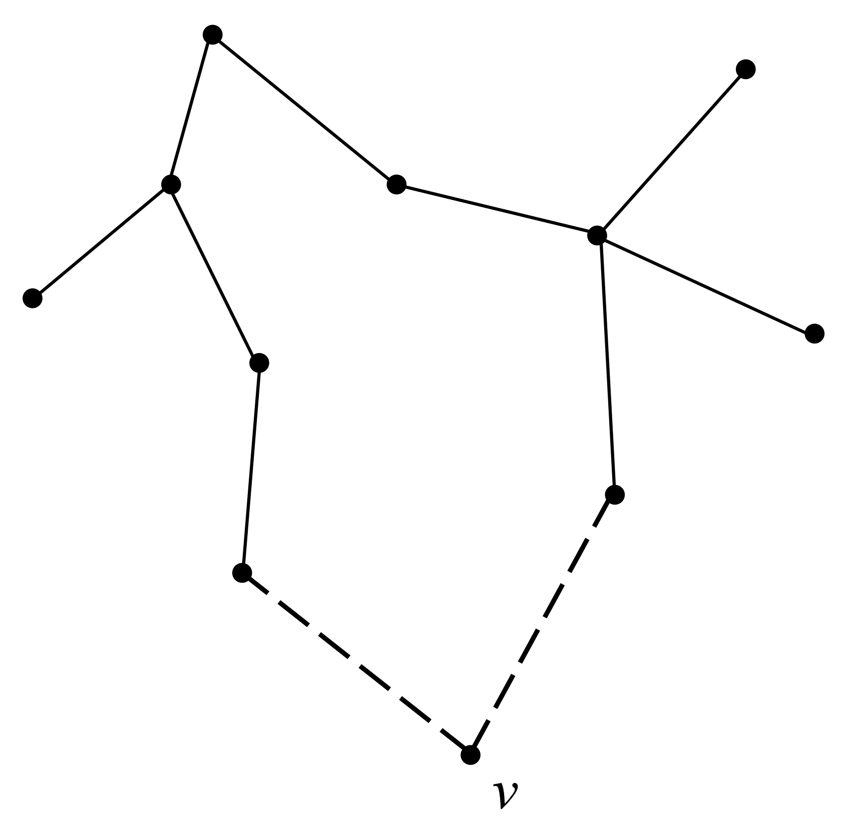
Figure 5 illustrates the iterative process of $k$ -opt, that is, the process of selecting the edges to be removed and the edges to be added. Suppose an initial tour has been obtained by a heuristic method, LK first randomly selects a point $p_{1}$ and let $i=1$ , then the edges to be removed and the edges to be added are selected alternately. When iterating to $p_{2i-1}$ , the edge $x_{i}$ needs to be selected. In fact, LK regards the selection of $x_{i}$ as the selection of $p_{2i}$ . The method of selecting $p_{2i}$ is to randomly select a point connected with $p_{2i-1}$ in the current TSP tour. Similarly, the selection of $y_{i}$ is regarded as the selection of $p_{2i+1}$ . The method for the algorithm to select $p_{2i+1}$ is to sequentially traverse the candidate set of $p_{2i}$ until it finds a city to be $p_{2i+1}$ that meets the constraints. The constraints of selecting $p_{2i}$ and $p_{2i+1}$ in LK are as follows:

•

$x_{i}$ and $y_{i}$ must share an endpoint, and so do $y_{i}$ and $x_{i+1}$ .
•

For $i\geq 2$ , if $p_{2i}$ connects back to $p_{1}$ for $y_{i}$ , the resulting configuration should be a tour.
•

$y_{i}$ is always chosen so that $g_{i}=\sum\limits_{j=1}^{i}(l(x_{j})-l(y_{j}))>0$ , where $g_{i}$ is the gain of replacing { $x_{1},x_{2},...,x_{i}$ } with { $y_{1},y_{2},...,y_{i}$ }. $l(\cdot)$ is the length of the corresponding edge.
•

Set { $x_{1},x_{2},...,x_{i}$ } and set { $y_{1},y_{2},...,y_{i}$ } are disjoint.

Let $g^{*}$ denote the best improvement in the current $k$ -opt process, and its initial value is set to 0. When $i\geq 2$ , LK sets $y^{\prime}=(p_{2i},p_{1})$ and calculates $g^{\prime}=g_{i-1}+l(x_{i})-l(y^{\prime})$ , and sets $g^{*}=g^{\prime}$ if $g^{\prime}>g^{*}$ . The iteration of $k$ -opt process in LK will stop when no link of $x_{i}$ and $y_{i}$ satisfy the above constraints or $g_{i}\leq{g^{*}}$ . When the iteration stops, if $g^{*}>0$ , then there is a $k$ -opt move that can improve the current TSP route. The whole algorithm will stop when the optimal solution of TSP is found or the maximum number of iterations is reached.

Main Improvements of LKH

The $\alpha$ -measure

LKH (Helsgaun 2000) proposed an $\alpha$ -value instead of distance as the measure for selecting and sorting cities in the candidate set, called $\alpha$ -measure, to improve the quality of the candidate set.

To explain the concept of $\alpha$ -value, we need to introduce the structure of 1-tree. A 1-tree for a graph $G(V,E)$ ( $V$ is the set of nodes, $E$ is the set of edges) is a spanning tree on the node set $V\backslash\{v\}$ combined with two edges from $E$ incident to a node $v$ , which is a special point chosen arbitrarily. Figure 6 shows a 1-tree. A minimum 1-tree is a 1-tree with minimum length, which can be found by determining the minimum spanning tree on $G$ and then adding an edge corresponding to the second nearest neighbor of one of the leaves of the tree. The leaf chosen is the one that has the longest second nearest neighbor distance. Obviously, the length of the minimum 1-tree is the lower bound of the optimal TSP solution. An important observation is that 70-80% of the edges in the optimal solution of TSP are also in the minimum 1-tree (Helsgaun 2000). Therefore, the LKH algorithm tries to define an $\alpha$ -value using the minimum 1-tree to replace the distance used by LK. The equation of calculating the $\alpha$ -value of an edge $(i,j)$ is as follows:

\alpha(i,j)=L(T^{+}(i,j))-L(T),

(9)

where $L(T)$ is the length of the minimum 1-tree of graph $G(V,E)$ and $L(T^{+}(i,j))$ is the length of the minimum 1-tree required to contain edge $(i,j)$ . That is, the $\alpha$ -value of an edge is equal to the length increased if the minimum 1-tree needs to include this edge. The LKH algorithm considers that an edge with smaller $\alpha$ -value is more likely to appear in the optimal solution. This $\alpha$ -measure has greatly improved the algorithm performance.

Penalties

In order to further enhance the advantage of the candidate set, LKH uses a method to maximize the lower bound of the optimal TSP solution by adding penalties (Held and Karp 1970). Concretely, a $\pi$ -value computed using a sub-gradient optimization method (Held and Karp 1971) is added to each node as penalties when calculating the distance between two nodes:

C(i,j)=d(i,j)+\pi_{i}+\pi_{j},

(10)

where $C(i,j)$ is the cost for a salesman from city $i$ to city $j$ after adding penalties, $d(i,j)$ is the distance between the two cities, and $\pi_{i},\pi_{j}$ are the penalties added to the two cities respectively. The penalties actually change the cost matrix of TSP. Note that this change does not change the optimal solution of the TSP, but it changes the minimum 1-tree. Suppose $L(T_{\pi})$ is the length of the minimum 1-tree after adding the penalties, then the lower bound $w(\pi)$ of the optimal solution can be calculated by Eq. 11, which is a function of set $\pi=[\pi_{1},...,\pi_{n}]$ :

w(\pi)=L(T_{\pi})-2\sum\limits_{i}\pi_{i}.

(11)

The lower bound $w(\pi)$ of the optimal solution is maximized, and after adding the penalties, the $\alpha$ -value is further improved for the candidate set.

In general, LKH (Helsgaun 2000) uses $\alpha$ -measure and penalties to improve the performance of LK. Moreover, the iteration of $k$ -opt process in LKH will stop immediately if a $k$ -opt move is found that can improve the current TSP tour. And LKH uses a 5-opt move as the basic move which means the maximum value of $k$ in the $k$ -opt process of LKH is 5.

More Experimental Results

In this section, we provide more experimental results, including the evaluation on the parameter sentivity of our algorithm, detailed performance comparision of VSR-LKH variants and LKH over the runtime, and the full results on all the 111 TSP benchmark instances.

Evaluation on Parameter Sensitivity

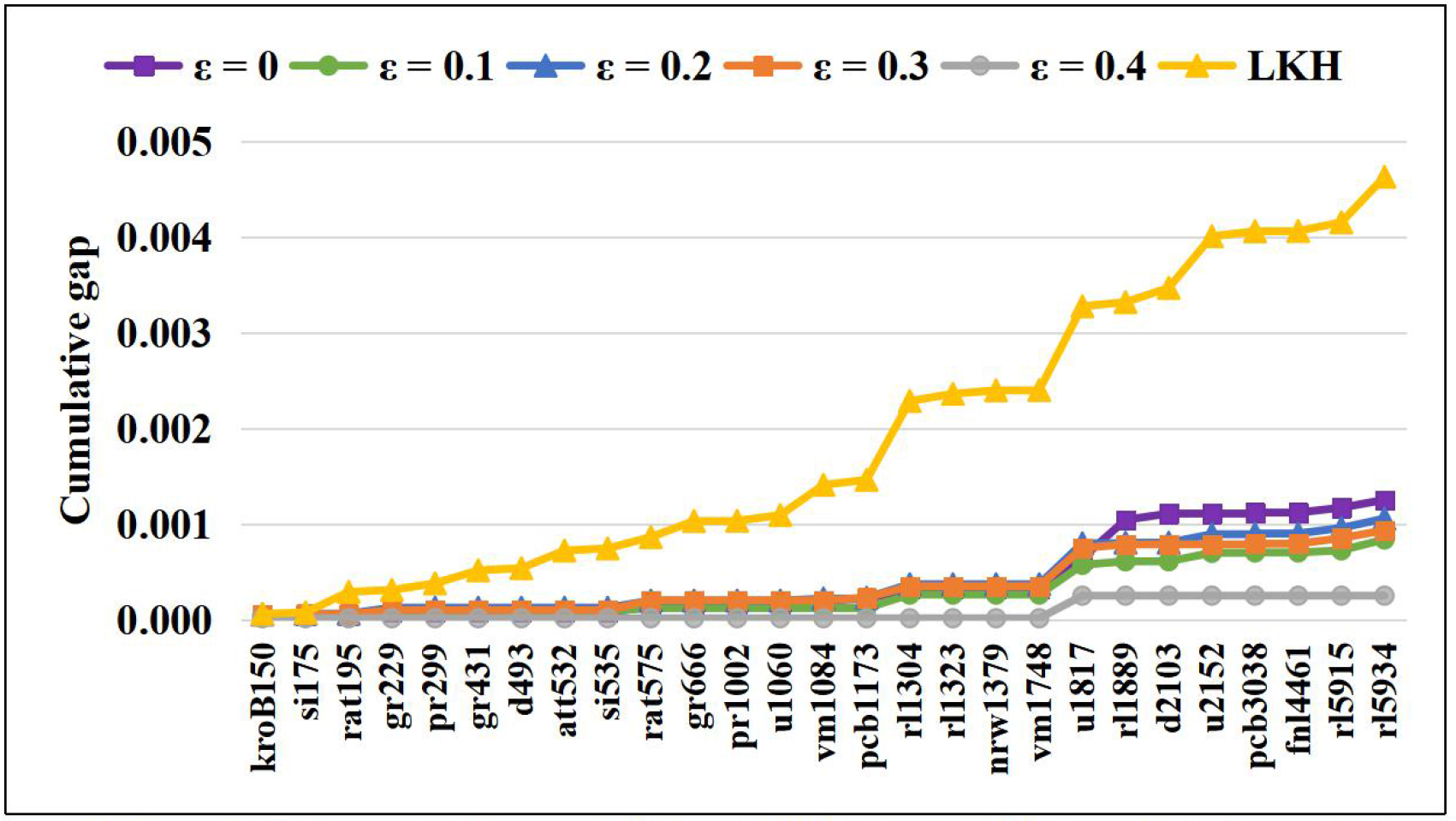
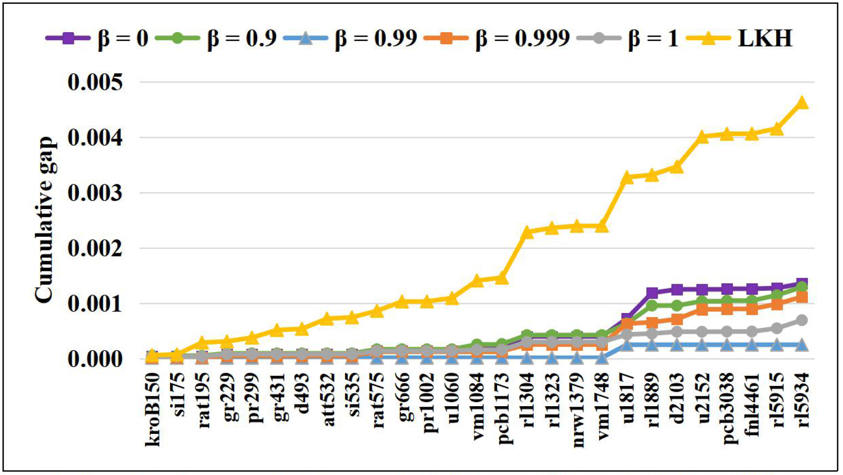
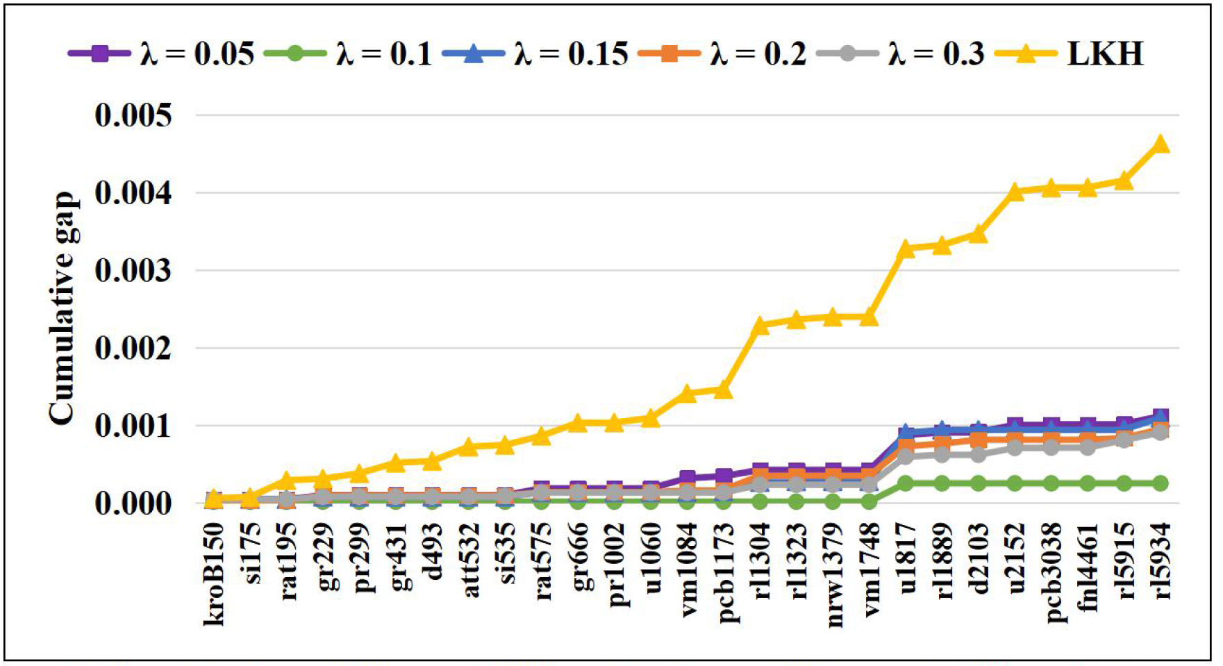
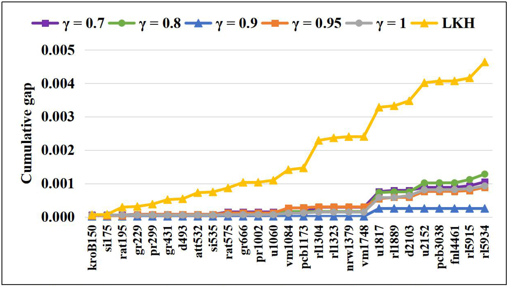
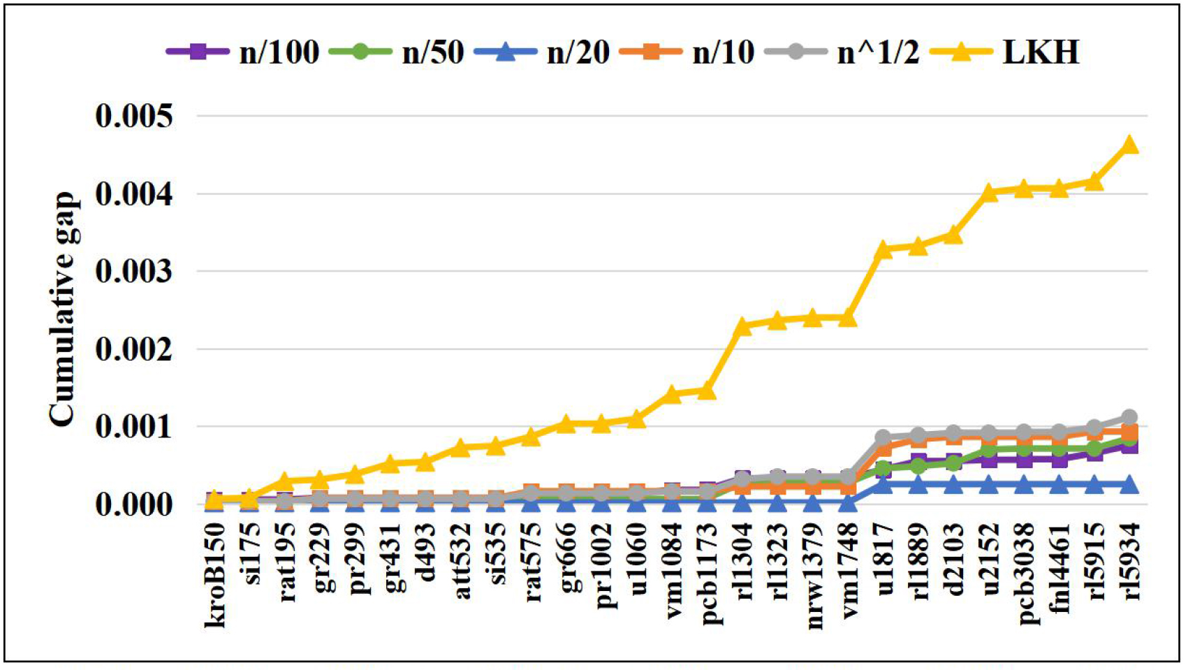
To evaluate the parameter sensitive as well as the robustness of VSR-LKH and choose appropriate reinforcement learning parameters, we do ablation study using different parameters include $\epsilon$ , $\beta$ , $\lambda$ , $\gamma$ and MaxNum. Note that when comparing each of the parameters, the others are fixed to default values ( $\epsilon=0.4$ , $\beta=0.99$ , $\lambda=0.1$ , $\gamma=0.9$ and $MaxNum=n/20$ , $n$ is the number of the cities).

The results are shown in Figure 7, and we can observe that the default parameters yield the best results. VSR-LKH with various parameters is significantly better than LKH, indicating that the proposed reinforcement learning method can always improve LKH. In addition, VSR-LKH with various parameters do not show significant difference on the results, indicating that VSR-LKH is robust and not very sensitive to the parameters.

Performance Comparison over Time

To analyze the optimization process of LKH and various variants of VSR-LKH (include VSR-LKH, TD-LKH, Q-LKH, SARSA-LKH, MC-LKH and FixQ-LKH) in solving the TSP, we randomly select six TSP instances (u574, u1060, u1817, fnl4461, rl5934 and rl11849) and compare their results over the runtime.

The results are shown in Figure 8. In the beginning of the iterations, LKH can yield better solutions than the reinforced algorithms. This is because the trial and error characteristics of reinforcement learning. However, the reinforced algorithms can surpass LKH in minutes or even seconds when solving these instances, demonstrating that the performance of VSR-LKH variants is better than LKH. In addition, FixQ-LKH also shows better results than LKH in Figure 8, indicating that the performance of LKH can be improved by only replacing the $\alpha$ -value with our initial Q-value to select and sort the candidate cities.

Full Experimental Results

We do full comparison of VSR-LKH and LKH on all the 111 symmetric TSP instances from the TSPLIB. We run 10 times for almost all instances except two super large instances, pla33810 and pla85900, due to the resource limit. For the two super large instances, we limit the maximum single runtime of LKH and VSR-LKH to 100,000 seconds and only run 3 times for the comparison.

Table LABEL:table3 shows the results. We can see that:

•

On all the 74 easy instances, both VSR-LKH and LKH can easily yield the optimal solution, and there is almost no difference on the running time.
•

On all the 37 hard instances, the proposed VSR-LKH greatly promotes the performance of the start-of-the-art algorithm LKH.

Table 3: Comparison of VSR-LKH and LKH on all 111 instances in TSPLIB (best results in bold).

NAME	Opt.	Method	Best	Average	Worst	Success	Time(s)	Trials
easy instances (a total of 74)
burma14	3323	LKH	Opt.	Opt.	Opt.	10/10	0.00	1.0
burma14	3323	VSR-LKH	Opt.	Opt.	Opt.	10/10	0.00	1.0
ulysses16	6859	LKH	Opt.	Opt.	Opt.	10/10	0.00	1.0
ulysses16	6859	VSR-LKH	Opt.	Opt.	Opt.	10/10	0.00	1.0
gr17	2085	LKH	Opt.	Opt.	Opt.	10/10	0.00	1.0
gr17	2085	VSR-LKH	Opt.	Opt.	Opt.	10/10	0.00	1.0
gr21	2707	LKH	Opt.	Opt.	Opt.	10/10	0.00	1.0
gr21	2707	VSR-LKH	Opt.	Opt.	Opt.	10/10	0.00	1.0
ulysses22	7013	LKH	Opt.	Opt.	Opt.	10/10	0.00	1.0
ulysses22	7013	VSR-LKH	Opt.	Opt.	Opt.	10/10	0.00	1.0
gr24	1272	LKH	Opt.	Opt.	Opt.	10/10	0.00	1.0
gr24	1272	VSR-LKH	Opt.	Opt.	Opt.	10/10	0.00	1.0
fri26	937	LKH	Opt.	Opt.	Opt.	10/10	0.00	1.0
fri26	937	VSR-LKH	Opt.	Opt.	Opt.	10/10	0.00	1.0
bayg29	1610	LKH	Opt.	Opt.	Opt.	10/10	0.00	1.0
bayg29	1610	VSR-LKH	Opt.	Opt.	Opt.	10/10	0.00	1.0
bays29	2020	LKH	Opt.	Opt.	Opt.	10/10	0.00	1.0
bays29	2020	VSR-LKH	Opt.	Opt.	Opt.	10/10	0.00	1.0
dantzig42	699	LKH	Opt.	Opt.	Opt.	10/10	0.00	1.0
dantzig42	699	VSR-LKH	Opt.	Opt.	Opt.	10/10	0.00	1.0
swiss42	1273	LKH	Opt.	Opt.	Opt.	10/10	0.01	1.0
swiss42	1273	VSR-LKH	Opt.	Opt.	Opt.	10/10	0.01	1.0
att48	10628	LKH	Opt.	Opt.	Opt.	10/10	0.01	1.0
att48	10628	VSR-LKH	Opt.	Opt.	Opt.	10/10	0.01	1.0
gr48	5046	LKH	Opt.	Opt.	Opt.	10/10	0.02	1.0
gr48	5046	VSR-LKH	Opt.	Opt.	Opt.	10/10	0.02	1.0
hk48	11461	LKH	Opt.	Opt.	Opt.	10/10	0.01	1.0
hk48	11461	VSR-LKH	Opt.	Opt.	Opt.	10/10	0.01	1.0
eil51	426	LKH	Opt.	Opt.	Opt.	10/10	0.02	1.0
eil51	426	VSR-LKH	Opt.	Opt.	Opt.	10/10	0.02	1.0
berlin52	7542	LKH	Opt.	Opt.	Opt.	10/10	0.01	1.0
berlin52	7542	VSR-LKH	Opt.	Opt.	Opt.	10/10	0.01	1.0
brazil58	25395	LKH	Opt.	Opt.	Opt.	10/10	0.01	1.0
brazil58	25395	VSR-LKH	Opt.	Opt.	Opt.	10/10	0.02	1.0
st70	675	LKH	Opt.	Opt.	Opt.	10/10	0.02	1.0
st70	675	VSR-LKH	Opt.	Opt.	Opt.	10/10	0.02	1.0
eil76	538	LKH	Opt.	Opt.	Opt.	10/10	0.02	1.0
eil76	538	VSR-LKH	Opt.	Opt.	Opt.	10/10	0.02	1.0
pr76	108159	LKH	Opt.	Opt.	Opt.	10/10	0.04	1.0
pr76	108159	VSR-LKH	Opt.	Opt.	Opt.	10/10	0.04	1.0
gr96	55209	LKH	Opt.	Opt.	Opt.	10/10	0.10	13.9
gr96	55209	VSR-LKH	Opt.	Opt.	Opt.	10/10	0.08	14.9
rat99	1211	LKH	Opt.	Opt.	Opt.	10/10	0.02	1.0
rat99	1211	VSR-LKH	Opt.	Opt.	Opt.	10/10	0.03	1.0
kroA100	21282	LKH	Opt.	Opt.	Opt.	10/10	0.04	1.0
kroA100	21282	VSR-LKH	Opt.	Opt.	Opt.	10/10	0.04	1.0
kroB100	22141	LKH	Opt.	Opt.	Opt.	10/10	0.05	1.2
kroB100	22141	VSR-LKH	Opt.	Opt.	Opt.	10/10	0.06	1.1
kroC100	20749	LKH	Opt.	Opt.	Opt.	10/10	0.04	1.0
kroC100	20749	VSR-LKH	Opt.	Opt.	Opt.	10/10	0.04	1.0
Continued on next page
kroD100	21294	LKH	Opt.	Opt.	Opt.	10/10	0.05	1.8
kroD100	21294	VSR-LKH	Opt.	Opt.	Opt.	10/10	0.05	1.0
kroE100	22068	LKH	Opt.	Opt.	Opt.	10/10	0.06	3.2
kroE100	22068	VSR-LKH	Opt.	Opt.	Opt.	10/10	0.06	2.9
rd100	7910	LKH	Opt.	Opt.	Opt.	10/10	0.02	1.0
rd100	7910	VSR-LKH	Opt.	Opt.	Opt.	10/10	0.03	1.0
eil101	629	LKH	Opt.	Opt.	Opt.	10/10	0.03	1.0
eil101	629	VSR-LKH	Opt.	Opt.	Opt.	10/10	0.03	1.0
lin105	14379	LKH	Opt.	Opt.	Opt.	10/10	0.02	1.0
lin105	14379	VSR-LKH	Opt.	Opt.	Opt.	10/10	0.02	1.0
pr107	44303	LKH	Opt.	Opt.	Opt.	10/10	0.15	1.0
pr107	44303	VSR-LKH	Opt.	Opt.	Opt.	10/10	0.19	1.0
gr120	6942	LKH	Opt.	Opt.	Opt.	10/10	0.03	1.0
gr120	6942	VSR-LKH	Opt.	Opt.	Opt.	10/10	0.04	1.5
pr124	59030	LKH	Opt.	Opt.	Opt.	10/10	0.06	1.0
pr124	59030	VSR-LKH	Opt.	Opt.	Opt.	10/10	0.08	1.0
bier127	118282	LKH	Opt.	Opt.	Opt.	10/10	0.04	1.0
bier127	118282	VSR-LKH	Opt.	Opt.	Opt.	10/10	0.06	1.0
ch130	6110	LKH	Opt.	Opt.	Opt.	10/10	0.06	1.0
ch130	6110	VSR-LKH	Opt.	Opt.	Opt.	10/10	0.07	1.0
pr136	96772	LKH	Opt.	Opt.	Opt.	10/10	0.12	1.0
pr136	96772	VSR-LKH	Opt.	Opt.	Opt.	10/10	0.12	1.0
gr137	69853	LKH	Opt.	Opt.	Opt.	10/10	0.06	1.0
gr137	69853	VSR-LKH	Opt.	Opt.	Opt.	10/10	0.08	1.0
pr144	58537	LKH	Opt.	Opt.	Opt.	10/10	0.47	1.0
pr144	58537	VSR-LKH	Opt.	Opt.	Opt.	10/10	0.53	1.0
ch150	6528	LKH	Opt.	Opt.	Opt.	10/10	0.08	1.7
ch150	6528	VSR-LKH	Opt.	Opt.	Opt.	10/10	0.12	13.0
kroA150	26524	LKH	Opt.	Opt.	Opt.	10/10	0.09	3.8
kroA150	26524	VSR-LKH	Opt.	Opt.	Opt.	10/10	0.07	1.0
pr152	73682	LKH	Opt.	Opt.	Opt.	10/10	0.87	29.4
pr152	73682	VSR-LKH	Opt.	Opt.	Opt.	10/10	0.68	18.3
u159	42080	LKH	Opt.	Opt.	Opt.	10/10	0.05	1.0
u159	42080	VSR-LKH	Opt.	Opt.	Opt.	10/10	0.05	1.0
brg180	1950	LKH	Opt.	Opt.	Opt.	10/10	0.09	4.1
brg180	1950	VSR-LKH	Opt.	Opt.	Opt.	10/10	0.17	6.9
d198	15780	LKH	Opt.	Opt.	Opt.	10/10	0.71	1.0
d198	15780	VSR-LKH	Opt.	Opt.	Opt.	10/10	0.97	1.0
kroA200	29368	LKH	Opt.	Opt.	Opt.	10/10	0.13	1.7
kroA200	29368	VSR-LKH	Opt.	Opt.	Opt.	10/10	0.14	1.0
kroB200	29437	LKH	Opt.	Opt.	Opt.	10/10	0.06	1.0
kroB200	29437	VSR-LKH	Opt.	Opt.	Opt.	10/10	0.08	1.0
gr202	40160	LKH	Opt.	Opt.	Opt.	10/10	0.07	1.0
gr202	40160	VSR-LKH	Opt.	Opt.	Opt.	10/10	0.10	1.4
ts225	126643	LKH	Opt.	Opt.	Opt.	10/10	0.11	1.0
ts225	126643	VSR-LKH	Opt.	Opt.	Opt.	10/10	0.11	1.0
tsp225	3916	LKH	Opt.	Opt.	Opt.	10/10	0.12	1.0
tsp225	3916	VSR-LKH	Opt.	Opt.	Opt.	10/10	0.18	2.7
pr226	80369	LKH	Opt.	Opt.	Opt.	10/10	0.14	1.0
pr226	80369	VSR-LKH	Opt.	Opt.	Opt.	10/10	0.19	4.5
gil262	2378	LKH	Opt.	Opt.	Opt.	10/10	0.23	10.6
gil262	2378	VSR-LKH	Opt.	Opt.	Opt.	10/10	0.17	2.4
Continued on next page
pr264	49135	LKH	Opt.	Opt.	Opt.	10/10	0.34	14.4
pr264	49135	VSR-LKH	Opt.	Opt.	Opt.	10/10	0.30	1.4
a280	2579	LKH	Opt.	Opt.	Opt.	10/10	0.11	1.0
a280	2579	VSR-LKH	Opt.	Opt.	Opt.	10/10	0.11	1.0
lin318	42029	LKH	Opt.	Opt.	Opt.	10/10	0.71	27.9
lin318	42029	VSR-LKH	Opt.	Opt.	Opt.	10/10	0.50	14.8
linhp318	41345	LKH	Opt.	Opt.	Opt.	10/10	0.23	11.9
linhp318	41345	VSR-LKH	Opt.	Opt.	Opt.	10/10	0.27	15.1
rd400	15281	LKH	Opt.	Opt.	Opt.	10/10	0.49	33.0
rd400	15281	VSR-LKH	Opt.	Opt.	Opt.	10/10	0.30	3.2
fl417	11861	LKH	Opt.	Opt.	Opt.	10/10	5.17	7.3
fl417	11861	VSR-LKH	Opt.	Opt.	Opt.	10/10	4.31	3.9
pr439	107217	LKH	Opt.	Opt.	Opt.	10/10	1.04	39.5
pr439	107217	VSR-LKH	Opt.	Opt.	Opt.	10/10	0.50	7.3
pcb442	50778	LKH	Opt.	Opt.	Opt.	10/10	0.37	8.2
pcb442	50778	VSR-LKH	Opt.	Opt.	Opt.	10/10	0.35	7.1
ali535	202339	LKH	Opt.	Opt.	Opt.	10/10	0.70	6.6
ali535	202339	VSR-LKH	Opt.	Opt.	Opt.	10/10	1.55	35.1
pa561	2763	LKH	Opt.	Opt.	Opt.	10/10	1.06	18.3
pa561	2763	VSR-LKH	Opt.	Opt.	Opt.	10/10	1.11	8.7
u574	36905	LKH	Opt.	Opt.	Opt.	10/10	1.78	149.9
u574	36905	VSR-LKH	Opt.	Opt.	Opt.	10/10	0.66	5.5
p654	34643	LKH	Opt.	Opt.	Opt.	10/10	13.73	22.9
p654	34643	VSR-LKH	Opt.	Opt.	Opt.	10/10	13.01	17.8
d657	48912	LKH	Opt.	Opt.	Opt.	10/10	1.03	33.5
d657	48912	VSR-LKH	Opt.	Opt.	Opt.	10/10	1.22	22.2
u724	41910	LKH	Opt.	Opt.	Opt.	10/10	3.12	125.4
u724	41910	VSR-LKH	Opt.	Opt.	Opt.	10/10	1.79	18.4
rat783	8806	LKH	Opt.	Opt.	Opt.	10/10	0.71	4.2
rat783	8806	VSR-LKH	Opt.	Opt.	Opt.	10/10	0.78	3.4
dsj1000	18660188	LKH	Opt.	Opt.	Opt.	10/10	56.10	441.4
dsj1000	18660188	VSR-LKH	Opt.	Opt.	Opt.	10/10	38.52	87.2
si1032	92650	LKH	Opt.	Opt.	Opt.	10/10	50.19	152.0
si1032	92650	VSR-LKH	Opt.	Opt.	Opt.	10/10	14.31	37.6
d1291	50801	LKH	Opt.	Opt.	Opt.	10/10	13.68	192.1
d1291	50801	VSR-LKH	Opt.	Opt.	Opt.	10/10	3.61	13.6
u1432	152970	LKH	Opt.	Opt.	Opt.	10/10	3.03	5.3
u1432	152970	VSR-LKH	Opt.	Opt.	Opt.	10/10	3.20	3.3
d1655	62128	LKH	Opt.	Opt.	Opt.	10/10	13.98	176.0
d1655	62128	VSR-LKH	Opt.	Opt.	Opt.	10/10	6.31	12.6
u2319	234256	LKH	Opt.	Opt.	Opt.	10/10	7.12	3.1
u2319	234256	VSR-LKH	Opt.	Opt.	Opt.	10/10	10.89	8.4
pr2392	378032	LKH	Opt.	Opt.	Opt.	10/10	8.09	5.8
pr2392	378032	VSR-LKH	Opt.	Opt.	Opt.	10/10	9.36	8.7
pla7397	23260728	LKH	Opt.	Opt.	Opt.	10/10	375.36	632.4
pla7397	23260728	VSR-LKH	Opt.	Opt.	Opt.	10/10	363.31	200.0
hard instances (a total of 37)
kroB150	26130	LKH	Opt.	26131.6	26132	2/10	0.40	128.4
kroB150	26130	VSR-LKH	Opt.	26130.4	26132	8/10	0.34	61.5
si175	21407	LKH	Opt.	21407.3	21408	7/10	10.31	105.9
si175	21407	VSR-LKH	Opt.	Opt.	Opt.	10/10	3.06	33.5
Continued on next page
rat195	2323	LKH	Opt.	2323.5	2328	9/10	0.28	55.0
rat195	2323	VSR-LKH	Opt.	Opt.	Opt.	10/10	0.15	2.8
gr229	134602	LKH	Opt.	134604.8	134616	8/10	0.57	107
gr229	134602	VSR-LKH	Opt.	Opt.	Opt.	10/10	0.45	57.5
pr299	48191	LKH	Opt.	48194.3	48224	9/10	0.64	51.7
pr299	48191	VSR-LKH	Opt.	Opt.	Opt.	10/10	0.41	6.2
gr431	171414	LKH	Opt.	171437.4	171534	4/10	7.48	339.1
gr431	171414	VSR-LKH	Opt.	Opt.	Opt.	10/10	4.66	76.4
d493	35002	LKH	Opt.	35002.8	35004	6/10	5.24	219.6
d493	35002	VSR-LKH	Opt.	Opt.	Opt.	10/10	1.14	10.2
att532	27686	LKH	Opt.	27691.1	27703	7/10	4.16	238.2
att532	27686	VSR-LKH	Opt.	Opt.	Opt.	10/10	1.18	17.8
si535	48450	LKH	Opt.	48451.1	48455	7/10	36.93	311.6
si535	48450	VSR-LKH	Opt.	Opt.	Opt.	10/10	27.62	144.0
rat575	6773	LKH	Opt.	6773.8	6774	2/10	3.73	526.9
rat575	6773	VSR-LKH	Opt.	Opt.	Opt.	10/10	3.69	151.3
gr666	294358	LKH	Opt.	294407.4	294476	5/10	6.67	467.5
gr666	294358	VSR-LKH	Opt.	Opt.	Opt.	10/10	3.33	45.2
pr1002	259045	LKH	Opt.	259045.6	259048	8/10	5.98	549.0
pr1002	259045	VSR-LKH	Opt.	Opt.	Opt.	10/10	2.25	22.1
u1060	224094	LKH	Opt.	224107.5	224121	5/10	142.07	663.3
u1060	224094	VSR-LKH	Opt.	Opt.	Opt.	10/10	5.68	13.7
vm1084	239297	LKH	Opt.	239372.6	239432	3/10	50.19	824.1
vm1084	239297	VSR-LKH	Opt.	Opt.	Opt.	10/10	12.71	116.6
pcb1173	56892	LKH	Opt.	56895.0	56897	4/10	7.15	844.0
pcb1173	56892	VSR-LKH	Opt.	Opt.	Opt.	10/10	7.80	291.1
rl1304	252948	LKH	Opt.	253156.4	253354	3/10	22.37	1170.0
rl1304	252948	VSR-LKH	Opt.	Opt.	Opt.	10/10	10.44	173.0
rl1323	270199	LKH	Opt.	270219.6	270324	6/10	17.55	718.8
rl1323	270199	VSR-LKH	Opt.	Opt.	Opt.	10/10	11.38	111.6
nrw1379	56638	LKH	Opt.	56640.0	56643	6/10	15.91	759.3
nrw1379	56638	VSR-LKH	Opt.	Opt.	Opt.	10/10	15.84	198.2
fl1400	20127	LKH	Opt.	20160.3	20164	1/10	5284.60	1372.9
fl1400	20127	VSR-LKH	Opt.	Opt.	Opt.	10/10	745.20	137.2
fl1577	22249	LKH	22254	22260.6	22263	0/10	2541.50	1577.0
fl1577	22249	VSR-LKH	22254	22254.0	22254	0/10	10770.90	1577.0
vm1748	336556	LKH	Opt.	336557.3	336569	9/10	22.82	1007.9
vm1748	336556	VSR-LKH	Opt.	Opt.	Opt.	10/10	14.08	47.0
u1817	57201	LKH	Opt.	57251.1	57274	1/10	116.39	1817.0
u1817	57201	VSR-LKH	Opt.	57214.5	57254	7/10	256.79	766.9
rl1889	316536	LKH	316549	316549.8	316553	0/10	109.78	1889.0
rl1889	316536	VSR-LKH	Opt.	Opt.	Opt.	10/10	26.30	91.9
d2103	80450	LKH	80454	80462.0	80473	0/10	216.48	2103.0
d2103	80450	VSR-LKH	Opt.	Opt.	Opt.	10/10	121.97	511.8
u2152	64253	LKH	Opt.	64287.7	64310	3/10	124.58	1614.0
u2152	64253	VSR-LKH	Opt.	Opt.	Opt.	10/10	65.41	185.8
pcb3038	137694	LKH	Opt.	137701.2	137741	4/10	128.20	2078.6
pcb3038	137694	VSR-LKH	Opt.	Opt.	Opt.	10/10	146.11	389.3
fl3795	28772	LKH	28813	28813.7	28815	0/10	54754.9	3795.0
fl3795	28772	VSR-LKH	Opt.	Opt.	Opt.	10/10	1805.20	89.4
fnl4461	182566	LKH	Opt.	182566.5	182571	9/10	79.40	923.1
fnl4461	182566	VSR-LKH	Opt.	Opt.	Opt.	10/10	71.94	94.8
Continued on next page
rl5915	565530	LKH	565544	565581.2	565593	0/10	494.81	5915.0
rl5915	565530	VSR-LKH	Opt.	Opt.	Opt.	10/10	438.50	851.4
rl5934	556045	LKH	556136	556309.8	556547	0/10	753.22	5934.0
rl5934	556045	VSR-LKH	Opt.	Opt.	Opt.	10/10	118.78	144.6
rl11849	923288	LKH	Opt.	923362.7	923532	2/10	3719.35	10933.4
rl11849	923288	VSR-LKH	Opt.	Opt.	Opt.	10/10	1001.11	751.9
usa13509	19982859	LKH	Opt.	19983103.4	19983569	1/10	4963.52	13509.0
usa13509	19982859	VSR-LKH	Opt.	19982930.2	19983029	5/10	25147.63	11900.0
brd14051	469385	LKH	469393	469398.3	469420	0/10	6957.07	14051.0
brd14051	469385	VSR-LKH	Opt.	469393.8	469403	1/10	37954.66	13581.3
d15112	1573084	LKH	1573085	1573142.7	1573223	0/10	7287.69	15112.0
d15112	1573084	VSR-LKH	Opt.	1573125.9	1573215	2/10	45642.47	13185.3
d18512	645238	LKH	645239	645260.6	645286	0/10	12399.27	18512.0
d18512	645238	VSR-LKH	645241	645261.6	645273	0/10	62662.90	18512.0
pla33810	66048945	LKH	66061689	66062670.0	66064532	0/3	100028.76	4294.3
pla33810	66048945	VSR-LKH	66049981	66055810.7	66063427	0/3	100028.91	1724.7
pla85900	142382641	LKH	142418173	142422390.7	142424554	0/3	100004.28	16486.3
pla85900	142382641	VSR-LKH	142393330	142396406.7	142402355	0/3	100018.84	2895.3

Combining Reinforcement Learning with Lin-Kernighan-Helsgaun Algorithm for the Traveling Salesman Problem

Abstract

Introduction

Related Work

Exact Algorithms.

Heuristic Algorithms.

Reinforcement Learning based Methods.

The Existing LKH Algorithm

The α𝛼\alpha-value.

Penalties.

The Proposed VSR-LKH Algorithm

Reinforcement Learning Framework

Initial Estimation of the State-action Function

The Reinforced Algorithms

Monte Carlo.

One-step TD.

Variable Strategy Reinforced k𝑘k-opt

Experimental Results

Experimental Setup

Q-value Evaluation

Comparison on Reinforcement Strategies

Final Comparison

Conclusion

Acknowledgments

References

Appendix

The Existing LKH Algorithms

The Lin-Kernighan Algorithm

Main Improvements of LKH

The α𝛼\alpha-measure

Penalties

More Experimental Results

Evaluation on Parameter Sensitivity

Performance Comparison over Time

Full Experimental Results

Combining Reinforcement Learning with Lin-Kernighan-Helsgaun Algorithm
for the Traveling Salesman Problem

The $\alpha$ -value.

Variable Strategy Reinforced $k$ -opt

The $\alpha$ -measure