Approximate analytical description of apparent horizons for initial data with momentum and spin

We construct analytical initial data for a slowly moving and rotating black hole for generic orientations of the linear momentum and the spin. We solve the Hamiltonian constraint approximately and work out the properties of the apparent horizon and show the dependence of its shape on the angle between the spin and the linear momentum. In particular a dimple, whose location depends on the mentioned angle, arises on the 2-sphere geometry of the apparent horizon. We exclusively work in the case of conformally flat initial metrics.

I Introduction

Since the first observation of black hole merger merger , there have been many observations of merger of compact objects via gravitational waves. The gravitational waves produced by these mergers are consistent with the numerical solutions of the field equations of General Relativity. Besides the highly accurate numerical results, it always pays to have approximate solutions of relativistic gravitating systems. Here we give an approximate analytical description of a self-gravitating system that has a conserved total energy, total spin and a linear momentum in an asymptotically flat spacetime. The initial configuration is expected to evolve and settle to a single rotating black hole after emitting some gravitational radiation.

The problem was studied in Gleiser in the case of vanishing linear momentum but with a nonzero spin; and in Dennison-Baumgarte in the case of vanishing spin with a nonzero linear momentum. See a remarkable exposition in kitap . Here we assume both of these quantities to be nonzero and pointing arbitrarily in three dimensional space. It will turn out that the shape of the apparent horizon depends on the angle between the linear momentum and the spin: even though at the next to leading order, the magnitude of the spin does not appear in the shape of the apparent horizon, its direction does. On the other hand, the shape of the apparent horizon depends on the magnitude of the linear momentum at the first order. The area of the apparent horizon does not depend on the angle between the spin and linear momentum. We also observe that a dimple arises on the 2-sphere geometry of the apparent horizon.

The layout of the paper is as follows. In the next section, we discuss briefly the constraint equations in General Relativity and present the Bowen-York method BY in finding solutions to the initial value problem. In section III, we give the approximate solution of the Hamiltonian constraint for a slowly rotating and moving black hole. In section IV, we compute the position of the apparent horizon as a function of the angle between the spin and the linear momentum.

II Initial data for a Black hole with momentum and spin

Assuming the usual ADM split of the metric ADM

$$ds^{2}=(N_{i}N^{i}-N^{2})dt^{2}+2N_{i}dtdx^{i}+\gamma_{ij}dx^{i}dx^{j},\hskip 28.45274pti,j\in(1,2,3),$$ (1)

the Einstein equations in vacuum without a cosmological constant split into constraints and the evolution equations. The constraint equations are given as

$$-^{\Sigma}R-K^{2}+K_{ij}K^{ij}=0,$$

$$-2D_{k}K_{i}^{k}+2D_{i}K=0,\leavevmode\nobreak\ \leavevmode\nobreak\ \leavevmode\nobreak\ \leavevmode\nobreak\ \leavevmode\nobreak\ \leavevmode\nobreak\ \leavevmode\nobreak\ \leavevmode\nobreak\ \leavevmode\nobreak\ \leavevmode\nobreak\ \leavevmode\nobreak\ \leavevmode\nobreak\ \leavevmode\nobreak\ \leavevmode\nobreak\$$ (2)

where $\Sigma$ is the Cauchy surface; $K_{ij}=K_{ij}(t,x^{k})$ is its extrinsic curvature defined as

$$K_{ij}=\frac{1}{2N}\Big{(}\dot{\gamma}_{ij}-D_{i}N_{j}-D_{j}N_{i}\Big{)},\hskip 28.45274pt\dot{\gamma}_{ij}=\frac{\partial}{\partial t}\gamma_{ij},$$ (3)

with the trace $K:=\gamma^{ij}K_{ij}$; and $D_{i}\gamma_{kl}=0$. For further details of the construction, including the evolution equations which we do not depict here, see the Appendix of our_dain_paper . Following Bowen-York BY , let us assume that $\Sigma$ is conformally flat with the metric

$$\gamma_{ij}=\psi^{4}f_{ij},\hskip 28.45274pt\psi>0,$$ (4)

with $f_{ij}$ denoting the flat metric in some generic coordinates. One also sets the extrinsic curvature of the hypersurface to be given as $K_{ij}=\psi^{-2}\hat{K}_{ij}$. Furthermore, we assume that $\Sigma$ is a maximally embedded hypersurface in the spacetime such that the trace of the extrinsic curvature vanishes 

$$K=0.$$ (5)

Under these conditions the Hamiltonian constraint reduces to a nonlinear elliptic equation

$$\hat{D}_{i}\hat{D}^{i}\psi=-\frac{1}{8}\psi^{-7}\hat{K}_{ij}^{2},$$ (6)

and the momentum constraint reduces to

$$\hat{D}^{i}\hat{K}_{ij}=0,$$ (7)

with $\hat{D}_{i}f_{jk}=0$. The momentum constraint equations can be solved easily, following BY , let us choose the $6$ parameter solution

$$\hat{K}_{ij}=\frac{3}{2r^{2}}\Big{(}p_{i}n_{j}+p_{j}n_{i}+(n_{i}n_{j}-f_{ij})p\cdot n\Big{)}+\frac{3}{r^{3}}{\cal{J}}^{l}n^{k}\Big{(}\varepsilon_{kil}n_{j}+\varepsilon_{kjl}n_{i}\Big{)},$$ (8)

where $n^{i}$ is the unit normal on a sphere of radius $r$. For other solutions, see Beig . Assuming the following asymptotic behavior for the conformal factor

$$\psi(r)=1+\frac{E}{2r}+{\mathcal{O}}(1/r^{2}),$$ (9)

one can easily show that (see Altas ) the $p^{i}$ in the solution (8) corresponds to the total conserved linear momentum via

$$P_{i}=\frac{1}{8\pi}\int_{S_{\infty}^{2}}dS\,n^{j}\,K_{ij}=\frac{1}{8\pi}\int_{S_{\infty}^{2}}dS\,n^{j}\,\hat{K}_{ij}.$$ (10)

Similarly one can show that $J_{i}$ corresponds to the total conserved angular momentum expressed in terms of the coordinates and the extrinsic curvature as

$$J_{i}=\frac{1}{16\pi}\varepsilon_{ijk}\int_{S_{\infty}^{2}}dS\,n_{l}\,\Big{(}x^{j}K^{kl}-x^{k}K^{jl}\Big{)}=\frac{1}{16\pi}\varepsilon_{ijk}\int_{S_{\infty}^{2}}dS\,n_{l}\,\Big{(}x^{j}\hat{K}^{kl}-x^{k}\hat{K}^{jl}\Big{)}.$$ (11)

Finally the ADM energy

$$E_{ADM}=\frac{1}{16\pi}\int_{S_{\infty}^{2}}dS\,n_{i}\,\Big{(}\partial_{j}h^{ij}-\partial_{i}h_{j}^{j}\Big{)},$$ (12)

becomes

$$E_{ADM}=-\frac{1}{2\pi}\int_{S_{\infty}^{2}}dS\,n^{i}\,\partial_{i}\psi,$$ (13)

and so using the asymptotic form (9) one finds $E_{ADM}=E$. This has been a brief description of the solution of the momentum constraints. Now, the important task is to solve the Hamiltonian constraint, which as we noted, is a nonlinear elliptic equation and thus, generically, it can only be solved numerically. But in the next section, we shall give an approximate solution for small momentum and small rotation.

III Initial data with small momentum and small spin

Computation of $\hat{K}_{ij}\hat{K}^{ij}$ (from equation (8)) yields

$$\hat{K}_{ij}\hat{K}^{ij}=\frac{9}{2r^{4}}\left(p^{2}+2(\vec{p}\cdot\vec{n})^{2}\right)+\frac{18}{r^{5}}\left(\vec{J}\times\vec{n}\right)\cdotp\vec{p}+\frac{18}{r^{6}}\left(\vec{J}\times\vec{n}\right)\cdotp\left(\vec{J}\times\vec{n}\right).$$ (14)

Without loss of generality, let us assume that the direction of the spin is the $\hat{k}$ direction, namely

$$\vec{J}=J\hat{k},$$ (15)

and $\vec{p}$ is lying in the $xz$ plane and given as

$$\vec{p}=p\sin\theta_{0}\hat{i}+p\cos\theta_{0}\hat{k}$$ (16)

with $\theta_{0}$ a fixed angle. To simplify the notation of the following discussion, let us denote

$$c_{1}:=\sin\theta_{0},\leavevmode\nobreak\ \leavevmode\nobreak\ \leavevmode\nobreak\ \leavevmode\nobreak\ \leavevmode\nobreak\ \leavevmode\nobreak\ \leavevmode\nobreak\ \leavevmode\nobreak\ c_{2}:=\cos\theta_{0}.$$ (17)

The Hamiltonian constraint, after these conventions becomes

$$\hat{D}_{i}\hat{D}^{i}\psi=\psi^{-7}\left(\frac{9Jp}{4r^{5}}c_{1}\sin\theta\sin\phi-\frac{9J^{2}}{4r^{6}}\sin^{2}\theta-\frac{9p^{2}}{16r^{4}}(1+2(c_{1}\sin\theta\cos\phi+c_{2}\cos\theta)^{2})\right).$$ (18)

As it clear from the right-hand side, the correct perturbative expansion in terms of the momentum and spin reads

$$\psi(r,\theta,\phi):=\psi^{(0)}+J^{2}\psi^{(J)}+p^{2}\psi^{(p)}+Jp\psi^{(Jp)}+\mathcal{O}(p^{4},J^{4},p^{2}J^{2}),$$ (19)

where the functions on the right-hand side depend on all coordinates $(r,\theta,\phi)$. At the lowest order, one has

$$\hat{D}_{i}\hat{D}^{i}\psi^{(0)}=0.$$ (20)

To proceed, let us discuss the boundary conditions that we shall employ. Following Brandt and Dennison-Baumgarte , we chose the following boundary conditions

$$\lim_{r\rightarrow\infty}\psi(r)=1,\leavevmode\nobreak\ \leavevmode\nobreak\ \leavevmode\nobreak\ \leavevmode\nobreak\ \leavevmode\nobreak\ \leavevmode\nobreak\ \leavevmode\nobreak\ \leavevmode\nobreak\ \leavevmode\nobreak\ \psi(r)>0,$$ (21)

and

$$\lim_{r\rightarrow\ 0}\psi(r)=\psi^{(0)}.$$ (22)

At the lowest order, the solution satisfying these boundary conditions reads

$$\psi^{(0)}=1+\frac{a}{r}.$$ (23)

Inserting (19) into (18), one arrives at three linear partial differential equations to be solved:

$$\hat{D}_{i}\hat{D}^{i}\psi^{(J)}=-\frac{9}{4}\sin^{2}\theta\frac{r}{(r+a)^{7}},\hskip 14.22636pt\hat{D}_{i}\hat{D}^{i}\psi^{(Jp)}=\frac{9}{4}c_{1}\sin\theta\sin\phi\frac{r^{2}}{(r+a)^{7}},$$ (24)

and also

$$\hat{D}_{i}\hat{D}^{i}\psi^{(p)}=-\frac{9}{16}\left(1+2(c_{1}\sin\theta\cos\phi+c_{2}\cos\theta)^{2}\right)\frac{r^{3}}{(r+a)^{7}}.$$ (25)

In finding the solutions to these equations, we will need the following spherical harmonics :

$$Y_{0}^{0}(\theta,\phi)=\frac{1}{\sqrt{4\pi}},\leavevmode\nobreak\ \leavevmode\nobreak\ \leavevmode\nobreak\ \leavevmode\nobreak\ \leavevmode\nobreak\ \leavevmode\nobreak\ \leavevmode\nobreak\ \leavevmode\nobreak\ \leavevmode\nobreak\ \leavevmode\nobreak\ \leavevmode\nobreak\ \leavevmode\nobreak\ \leavevmode\nobreak\ \leavevmode\nobreak\ \leavevmode\nobreak\ Y_{1}^{0}(\theta,\phi)=\sqrt{\frac{3}{4\pi}}\cos\theta,\leavevmode\nobreak\ \leavevmode\nobreak\ \leavevmode\nobreak\ \leavevmode\nobreak\ \leavevmode\nobreak\ \leavevmode\nobreak\ Y_{2}^{0}(\theta,\phi)=\sqrt{\frac{5}{16\pi}}(3\cos^{2}\theta-1),$$ (26)

$$Y_{1}^{-1}(\theta,\phi)=\sqrt{\frac{3}{4\pi}}\sin\theta\sin\phi,\leavevmode\nobreak\ \leavevmode\nobreak\ \leavevmode\nobreak\ \leavevmode\nobreak\ Y_{2}^{1}(\theta,\phi)=\sqrt{\frac{15}{4\pi}}\sin\theta\cos\theta\cos\phi,\leavevmode\nobreak\ \leavevmode\nobreak\ \leavevmode\nobreak\ \leavevmode\nobreak\ Y_{1}^{1}(\theta,\phi)=\sqrt{\frac{3}{4\pi}}\sin\theta\cos\phi.$$

Then ansatz for $\psi^{(J)}$ can be taken as

$$\psi^{(J)}(r,\theta,\phi)=\psi_{0}^{(J)}(r)Y_{0}^{0}(\theta,\phi)+\psi_{1}^{(J)}(r)Y_{2}^{0}(\theta,\phi),$$ (27)

which upon insertion to the first equation of (24) yields two ordinary differential equations equations

$$\frac{d}{dr}\bigl{(}r^{2}\frac{d\psi_{0}^{(J)}(r)}{dr}\bigr{)}=-3\sqrt{\pi}\frac{r^{3}}{(r+a)^{7}},\hskip 14.22636pt\frac{d}{dr}\bigl{(}r^{2}\frac{d\psi_{1}^{(J)}(r)}{dr}\bigr{)}-6\psi_{1}^{(J)}(r)=3\sqrt{\frac{\pi}{5}}\frac{r^{3}}{(r+a)^{7}}.$$ (28)

The solution obeying the boundary conditions (21) reads

$$\psi^{(J)}(r,\theta,\phi)=\frac{\left(a^{4}+5a^{3}r+10a^{2}r^{2}+5ar^{3}+r^{4}\right)}{40a^{3}(a+r)^{5}}-\frac{r^{2}}{40a(a+r)^{5}}(3\cos^{2}\theta-1).$$ (29)

Similarly setting

$$\psi^{(Jp)}(r,\theta,\phi)=\psi_{0}^{(Jp)}(r)Y_{0}^{0}(\theta,\phi)+\psi_{1}^{(Jp)}(r)Y_{1}^{-1}(\theta,\phi)$$ (30)

in the second equation of (24), one finds that $\psi_{0}^{(Jp)}(r)=0$ satisfies the boundary conditions; and the $\psi_{1}^{(Jp)}(r)$ piece satisfies

$$\frac{d}{dr}\bigl{(}r^{2}\frac{d\psi_{1}^{(Jp)}(r)}{dr}\bigr{)}-2\psi_{1}^{(Jp)}(r)=\frac{3\sqrt{3\pi}}{2}c_{1}\frac{r^{4}}{(r+a)^{7}}$$ (31)

of which the solution can be found and one has

$$\psi^{(Jp)}(r,\theta,\phi)=-\frac{c_{1}r\left(a^{2}+5ar+10r^{2}\right)}{80a(a+r)^{5}}\sin\theta\sin\phi.$$ (32)

Finally, let us do the $\psi^{(p)}(r,\theta,\phi)$ part which is slightly more complicated. One sets

$$\psi^{(p)}=\psi_{0}^{(p)}(r)Y_{0}^{0}(\theta,\phi)+\psi_{1}^{(p)}(r)Y_{1}^{1}(\theta,\phi)^{2}+\psi_{2}^{(p)}(r)Y_{2}^{1}(\theta,\phi)+\psi_{3}^{(p)}(r)Y_{1}^{0}(\theta,\phi)^{2}$$ (33)

to arrive at four equations, two of which are

$$\frac{d}{dr}\bigl{(}r^{2}\frac{d\psi_{0}^{(p)}}{dr}\bigr{)}+\frac{3}{\sqrt{\pi}}(\psi_{1}^{(p)}+\psi_{3}^{(p)})=-\frac{9}{8}\sqrt{\pi}\frac{r^{5}}{(r+a)^{7}},$$ (34)

and

$$\frac{d}{dr}\bigl{(}r^{2}\frac{d\psi_{1}^{(p)}}{dr}\bigr{)}-6\psi_{1}^{(p)}=-\frac{3}{2}\pi c_{1}^{2}\frac{r^{5}}{(r+a)^{7}}.$$ (35)

$\psi_{2}^{(p)}(r)$ equation can be obtained from (35) with the replacement $c_{1}^{2}\rightarrow\sqrt{\frac{3}{5\pi}}c_{1}c_{2}$ and $\psi_{3}^{(p)}(r)$ equation can be obtained from (35) via $c_{1}^{2}\rightarrow c_{2}^{2}$. The solutions read, respectively, as follows

$$\psi_{0}^{(p)}(r) = -\frac{\sqrt{\pi}\left(84a^{6}+378a^{5}r+653a^{4}r^{2}+514a^{3}r^{3}+142a^{2}r^{4}-35ar^{5}-25r^{6}\right)}{80ar^{2}(a+r)^{5}}$$ (36)

$$-\frac{21\sqrt{\pi}a}{20r^{3}}\log\frac{a}{a+r},$$

and

$$\psi_{1}^{(p)}(r) = \frac{\pi c_{1}^{2}\left(84a^{5}+378a^{4}r+658a^{3}r^{2}+539a^{2}r^{3}+192ar^{4}+15r^{5}\right)}{40r^{2}(a+r)^{5}}$$ (37)

$$+\frac{21\pi ac_{1}^{2}}{10r^{3}}\log\frac{a}{r+a},$$

from which one can find $\psi^{(p)}$, but we do not depict it here since it is a little long.

Recall that for the ADM energy computation, we need the dominant terms up to and including $\mathcal{O}(\frac{1}{r})$ in $\psi(r,\theta,\phi)$. Collecting these parts in the above solutions, one gets

$$\psi(r)=1+\frac{a}{r}+\frac{J^{2}}{40a^{3}r}+\frac{5p^{2}}{32ar}+\mathcal{O}(\frac{1}{r^{2}}).$$ (38)

Therefore from (9), the ADM energy of the solution reads

$$E_{\text{ADM}}=2a+\frac{J^{2}}{20a^{3}}+\frac{5p^{2}}{16a}.$$ (39)

Observe that the $Jp$ term does not contribute to the energy since it is of $\mathcal{O}(\frac{1}{r^{2}})$.

Next, as in Dennison-Baumgarte , let us express the ADM energy in terms of the irreducible mass $M_{\text{irr}}$ which is definedChris as

$$M_{\text{irr}}:=\sqrt{\frac{A}{16\pi}}$$ (40)

with $A$ being the area of a section of the event horizon. But as the event horizon is a $4$ dimensional concept, which cannot be derived from the $3$ dimensional initial data, we will approximate this with the area of the apparent horizon, $A_{\text{AH}}$, following Dennison-Baumgarte .

IV Computation of the apparent horizon for the boosted, rotating solutions

Let $S$ be a $2$ dimensional subspace of $\Sigma$ and $s^{i}$ be the normalized unit vector of $S$, i.e. $s^{i}s_{i}=1$. Then the metric on $S$ is the pull-back metric from $\Sigma$ given as

$$m_{ij}:=\gamma_{ij}-s_{i}s_{j}.$$ (41)

The expansion of the null geodesic congruence vanishes at the apparent horizon by definition, i.e. it is a marginally trapped surface and the defining equation becomes

$$\left(\gamma^{ij}-s^{i}s^{j}\right)\left(D_{i}s_{j}-K_{ij}\right)=0.$$ (42)

Assuming the surface to be defined as a level set of a function

$$\Phi:=r-h(\theta,\phi)=0,$$ (43)

then the normal one-form reads

$$s_{i}:=\lambda m_{i}=\lambda\partial_{i}\varPhi,$$ (44)

which explicitly becomes

$$s_{i}=\lambda\left(1,-\partial_{\theta}h,-\partial_{\phi}h\right).$$ (45)

Recall that the metric on $\Sigma$ is

$$\gamma_{ij}=\psi^{4}\begin{pmatrix}1&0&0\\ 0&r^{2}&0\\ 0&0&r^{2}\sin^{2}\theta\end{pmatrix},$$ (46)

then one has

$$s^{i}=\lambda\left(\gamma^{rr},-\gamma^{\theta\theta}\partial_{\theta}h,-\gamma^{\phi\phi}\partial_{\phi}h\right),$$ (47)

and

$$\lambda=\Big{(}\gamma^{rr}+\gamma^{\theta\theta}(\partial_{\theta}h)^{2}+\gamma^{\phi\phi}(\partial_{\phi}h)^{2}\Big{)}^{-1/2}.$$ (48)

Equation (42) reads more explicitly as

$$\gamma^{ij}\partial_{i}m_{j}-\gamma^{ij}\Gamma_{ij}^{k}m_{k}-\lambda^{2}m^{i}m^{j}\partial_{i}m_{j}+\lambda^{2}m^{i}m^{j}m_{k}\Gamma_{ij}^{k}+\lambda m^{i}m^{j}K_{ij}=0,$$ (49)

where we have used $\gamma^{ij}K_{ij}=K=0$. After working out each piece, one arrives at

$$-\gamma^{\theta\theta}\partial_{\theta}^{2}h-\gamma^{\phi\phi}\partial_{\phi}^{2}h-\frac{1}{2}\Bigl{(}(\gamma^{rr})^{2}\partial_{r}\gamma_{rr}-\gamma^{\theta\theta}\gamma^{rr}\partial_{r}\gamma_{\theta\theta}-\gamma^{\phi\phi}\gamma^{rr}\partial_{r}\gamma_{\phi\phi}+\partial_{\theta}h\gamma^{\phi\phi}\gamma^{\theta\theta}\partial_{\theta}\gamma_{\phi\phi}\Bigr{)}$$

$$+\lambda^{2}\Bigl{(}(\gamma^{\theta\theta})^{2}(\partial_{\theta}h)^{2}\partial_{\theta}^{2}h+(\gamma^{\phi\phi})^{2}(\partial_{\phi}h)^{2}\partial_{\phi}^{2}h+2\gamma^{\phi\phi}\gamma^{\theta\theta}\partial_{\phi}h\partial_{\theta}h\partial_{\theta}\partial_{\phi}h\Bigr{)}$$

$$+\frac{\lambda^{2}}{2}\Bigl{(}(\gamma^{rr})^{3}\partial_{r}\gamma_{rr}+(\gamma^{\theta\theta})^{2}\gamma^{rr}(\partial_{\theta}h)^{2}\partial_{r}\gamma_{\theta\theta}+(\gamma^{\phi\phi})^{2}\gamma^{rr}(\partial_{\phi}h)^{2}\partial_{r}\gamma_{\phi\phi}$$

$$\leavevmode\nobreak\ \leavevmode\nobreak\ \leavevmode\nobreak\ \leavevmode\nobreak\ \leavevmode\nobreak\ \leavevmode\nobreak\ \leavevmode\nobreak\ \leavevmode\nobreak\ \leavevmode\nobreak\ \leavevmode\nobreak\ \leavevmode\nobreak\ \leavevmode\nobreak\ \leavevmode\nobreak\ -(\partial_{\phi}h)^{2}\partial_{\theta}h(\gamma^{\phi\phi})^{2}\gamma^{\theta\theta}\partial_{\theta}\gamma_{\phi\phi}\Bigr{)}$$

$$+\lambda\Bigl{(}(\gamma^{rr})^{2}K_{rr}+(\gamma^{\theta\theta})^{2}(\partial_{\theta}h)^{2}K_{\theta\theta}+(\gamma^{\phi\phi})^{2}(\partial_{\phi}h)^{2}K_{\phi\phi}-2\gamma^{rr}\gamma^{\theta\theta}\partial_{\theta}hK_{r\theta}$$

$$\leavevmode\nobreak\ \leavevmode\nobreak\ \leavevmode\nobreak\ \leavevmode\nobreak\ \leavevmode\nobreak\ \leavevmode\nobreak\ \leavevmode\nobreak\ \leavevmode\nobreak\ \leavevmode\nobreak\ \leavevmode\nobreak\ \leavevmode\nobreak\ \leavevmode\nobreak\ \leavevmode\nobreak\ \leavevmode\nobreak\ -2\gamma^{rr}\gamma^{\phi\phi}\partial_{\phi}hK_{r\phi}+2\gamma^{\theta\theta}\gamma^{\phi\phi}\partial_{\theta}h\partial_{\phi}hK_{\theta\phi}\Bigr{)}=0.$$ (50)

An exact solution to this equation is beyond reach and we do not really need it. All we need is an approximate solution of the form

$$h(\theta,\phi)=h^{0}+ph^{p}+Jh^{J}+\mathcal{O}(p^{2},J^{2},Jp),$$ (51)

where

$$\partial_{r}h=0,\leavevmode\nobreak\ \leavevmode\nobreak\ \leavevmode\nobreak\ \leavevmode\nobreak\ \leavevmode\nobreak\ \leavevmode\nobreak\ \partial_{r}h^{0}=0=\partial_{\theta}h^{0}=\partial_{\phi}h^{0}.$$ (52)

Note that to compute the area of the apparent horizon and the irreducible mass up to and including the $\mathcal{O}(p^{2},J^{2},Jp)$ terms, one only needs the shape of the horizon up to and including the $\mathcal{O}(p,J)$ terms which becomes clear when one studies the area integral. [See alsoDennison-Baumgarte .] Ignoring the higher order terms such as $(\partial_{\theta}h)^{2}$, $(\partial_{\phi}h)^{2}$ and $\partial_{\theta}h\partial_{\phi}h$, the apparent horizon equation becomes

$$-\gamma^{\theta\theta}\partial_{\theta}^{2}h-\gamma^{\phi\phi}\partial_{\phi}^{2}h-\frac{1}{2}\left((\gamma^{rr})^{2}\partial_{r}\gamma_{rr}-\gamma^{\theta\theta}\gamma^{rr}\partial_{r}\gamma_{\theta\theta}-\gamma^{\phi\phi}\gamma^{rr}\partial_{r}\gamma_{\phi\phi}+\partial_{\theta}h\gamma^{\phi\phi}\gamma^{\theta\theta}\partial_{\theta}\gamma_{\phi\phi}\right)$$

$$\leavevmode\nobreak\ \leavevmode\nobreak\ \leavevmode\nobreak\ \leavevmode\nobreak\ \leavevmode\nobreak\ \leavevmode\nobreak\ \leavevmode\nobreak\ \leavevmode\nobreak\ \leavevmode\nobreak\ \leavevmode\nobreak\ \leavevmode\nobreak\ \leavevmode\nobreak\ \leavevmode\nobreak\ \leavevmode\nobreak\ \leavevmode\nobreak\ \leavevmode\nobreak\ \leavevmode\nobreak\ \leavevmode\nobreak\ \leavevmode\nobreak\ \leavevmode\nobreak\ +\frac{\lambda^{2}}{2}(\gamma^{rr})^{3}\partial_{r}\gamma_{rr}+\lambda\gamma^{rr}\left(\gamma^{rr}K_{rr}-2\gamma^{\theta\theta}\partial_{\theta}hK_{r\theta}-2\gamma^{\phi\phi}\partial_{\phi}hK_{r\phi}\right)=0.$$ (53)

To proceed, we need the components of the extrinsic curvature in the $(r,\theta,\phi)$ coordinates. After coordinate transformations, one finds

$$\hat{K}_{rr}=\frac{3p}{r^{2}}\Big{(}c_{1}\sin\theta\cos\phi+c_{2}\cos\theta\Big{)},\,\,\,\hat{K}_{r\theta}=\frac{3p}{2r}\Big{(}c_{1}\cos\theta\cos\phi-c_{2}\sin\theta\Big{)},$$ (54)

and

$$\hat{K}_{r\phi}=-\frac{3p}{2r}c_{1}\sin\theta\sin\phi+\frac{3J}{r^{2}}\sin^{2}\theta.$$ (55)

Therefore the resulting equation is

$$\partial_{\theta}^{2}h+\frac{1}{\sin^{2}\theta}\partial_{\phi}^{2}h+\cot\theta\partial_{\theta}h-2r-4r^{2}\frac{\partial_{r}\psi}{\psi}+\frac{6J}{\psi^{4}r^{2}}\partial_{\phi}h-\frac{3p}{\psi^{4}}\Big{(}c_{1}\sin\theta\cos\phi+c_{2}\cos\theta\Big{)}=0.$$ (56)

At order, $\mathcal{O}(p^{0},J^{0})$, this equation yields

$$1+2r\frac{\partial_{r}\psi}{\psi}=0,$$ (57)

where $\psi=1+\frac{a}{r}$ . And setting $r=h$, one finds

$$h^{0}=a.$$ (58)

This explains the physical meaning of the parameter $a$: it is the location of the apparent horizon at the lowest order. The next order contribution, which we shall find below, will be perturbations to this location. At $\mathcal{O}(p)$ and $\mathcal{O}(J)$ we have the following equations, respectively

$$\partial_{\theta}^{2}h^{p}+\frac{1}{\sin^{2}\theta}\partial_{\phi}^{2}h^{p}+\cot\theta\partial_{\theta}h^{p}-h^{p}-\frac{3}{16}\Big{(}c_{1}\sin\theta\cos\phi+c_{2}\cos\theta\Big{)}=0,$$ (59)

and

$$\partial_{\theta}^{2}h^{J}+\frac{1}{\sin^{2}\theta}\partial_{\phi}^{2}h^{J}+\cot\theta\partial_{\theta}h^{J}-h^{J}=0.$$ (60)

These are linear PDE’s and a close scrunity shows that $h^{J}$ equation is the homogenous Helmholtz equation on a sphere ($S^{2}$), while $h^{P}$ equation is the inhomogeneous Helmholtz equation with a non-trivial source. So the next task is to find everywhere finite solutions of the following equation

$$\left({\vec{\nabla}}_{S^{2}}^{2}+k\right)f\left(\theta,\phi\right)=g\left(\theta,\phi\right),$$ (61)

where ${\vec{\nabla}}_{S^{2}}^{2}$ is the Laplacian on $S^{2}$:

$${\vec{\nabla}}_{S^{2}}^{2}=\partial_{\theta}^{2}+\cot\theta\partial_{\theta}+\frac{1}{\sin^{2}\theta}\partial_{\phi}^{2}.$$ (62)

It is clear that the Green’s function technique is the most suitable approach to this problem. For the Helmholtz operator on the sphere, the Green function $G(\hat{x},\hat{x}^{\prime})$ is defined as

$$\left({\vec{\nabla}}_{S^{2}}^{2}+\lambda(\lambda+1)\right)G(\hat{x},\hat{x}^{\prime})=\delta^{(2)}(\hat{x}-\hat{x}^{\prime}),$$ (63)

which can be found to be (for example, see Green )

$$G(\hat{x},\hat{x}^{\prime})=\frac{1}{4\sin\pi\lambda}\sum_{n=0}^{\infty}\frac{1}{\left(n!\right)^{2}}\frac{\Gamma(n-\lambda)}{\Gamma(-\lambda)}\frac{\Gamma(n+\lambda+1)}{\Gamma(\lambda+1)}\left(\frac{1+\hat{x}\cdot\hat{x^{\prime}}}{2}\right)^{n},$$ (64)

where $\hat{x}=\sin\theta\cos\phi\hat{i}+\sin\theta\sin\phi\hat{j}+\cos\theta\hat{k}$ and $\hat{x}^{{}^{\prime}}$ is a similar expression with some other $\theta$ and $\phi$. Employing this Green’s function with $\lambda=\frac{-1+i\sqrt{3}}{2}$ one finds

$$h^{p}=-\frac{1}{16}\left(c_{1}\sin\theta\cos\phi+c_{2}\cos\theta\right)$$ (65)

and $h^{J}=0$. Therefore the apparent horizon is located at

$$r=h(\theta,\phi)=a-\frac{1}{16}\Big{(}\vec{p}\cdot\hat{J}\cos\theta+|\vec{p}\wedge\hat{J}\rvert\sin\theta\cos\phi\Big{)},$$ (66)

where $\hat{J}=\frac{\vec{J}}{J}$. In the limit $\theta_{0}=0$, $h$ reduces to the form given in Dennison-Baumgarte , that is $h(\theta)=a-\frac{p}{16}\cos\theta$; and the apparent horizon in this axially symmetric case is a squashed sphere from the North pole. Note that the shape of the apparent horizon 66 at this order does not depend on the magnitude of the spin but it does depend on its orientation with respect to the linear momentum. In figure 1, we plot the apparent horizon. To be able to see the dimple clearly in the whole figure, we have chosen a high momentum value.

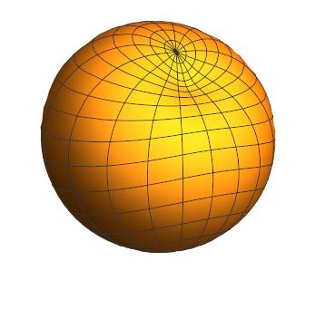
Figure 1: The shape of the apparent horizon when the angle between $\vec{p}$ and $\vec{J}$ is 45 degrees; and to be able to see the dimple, we have chosen $p/a=8\sqrt{2}$ which is outside the validity of the approximation we have worked with. But the dimple exists for even small $p$.

Let us now evaluate the area of the apparent horizon from the formula

$$A_{\text{AH}}=\intop_{0}^{2\pi}d\phi\intop_{0}^{\pi}d\theta\sqrt{\det m},$$ (67)

which at the order we are working yields

$$A_{\text{AH}}=\intop_{0}^{2\pi}d\phi\intop_{0}^{\pi}d\theta\thinspace\sin\theta\thinspace\psi^{4}\thinspace h^{2}\left(1+\frac{1}{h^{2}}\left(\partial_{\theta}h\right)^{2}+\frac{1}{h^{2}\sin^{2}\theta}\left(\partial_{\phi}h\right)^{2}\right)^{1/2}.$$ (68)

This is a pretty long computation since the conformal factor is quite complicated. But at the end, one finds

$$A_{\text{AH}}=64\pi a^{2}+4\pi p^{2}+\frac{11\pi J^{2}}{5a^{2}}.$$ (69)

Note that the angle between the spin and the linear momentum does not appear in the area. Then the irreducible mass $M_{\text{irr}}$ reads

$$M_{\text{irr}}=2a+\frac{p^{2}}{16a}+\frac{11J^{2}}{320a^{3}}.$$ (70)

Comparing with $E_{ADM}$ we have

$$E_{\text{ADM}}=M_{\text{irr}}+\frac{p^{2}}{2M_{\text{irr}}}+\frac{J^{2}}{8M_{\text{irr}}^{3}}$$ (71)

which matches the slow momentum and spin limit of the result in Chris .

V Conclusions

Momentum constraints in General Relativity are easily solved with the method of Bowen-York while the Hamiltonian constraint is a nontrivial elliptic equation. Here, extending earlier works Gleiser , Dennison-Baumgarte we gave an approximate analytical solution that describes a spinning and moving system with a conserved spin and linear momentum pointing in arbitrary directions. We computed the properties of the apparent horizon, such as its shape and surface area and showed the dependence of the shape on the angle between the spin and the linear momentum. We calculated the relation between the conserved quantities such as the ADM mass, the spin, the linear momentum and the irreducible mass. The area of the apparent horizon does not depend on the angle between the spin and the linear momentum, but a dimple arises in the apparent horizon whose location depends on this angle.

References

(1) B. P. Abbott et al. [LIGO Scientific
and Virgo Collaborations], Observation of Gravitational Waves from
a Binary Black Hole Merger, Phys. Rev. Lett. 116, no.
6, 061102 (2016).
(2) R. J. Gleiser, C. O. Nicasio, R. H. Price, and
J. Pullin, Evolving the Bowen-York initial data for spinning black
holes, Phys. Rev. D 57, 3401, (1998).
(3) K. A. Dennison, T. W. Baumgarte, and
H. P. Pfeiffer, Approximate initial data for binary black holes, Phys.
Rev. D 74, 064016, (2006).
(4) T. Baumgarte and S. Shapiro, Numerical Relativity:
Solving Einstein’s Equations on the Computer. Cambridge: Cambridge
University Press (2010).
(5) J. M. Bowen and J. W. York, Jr., Time asymmetric
initial data for black holes and black hole collisions, Phys. Rev.
D 21 , 2047-2056 (1980).
(6) R. Arnowitt, S. Deser and C. Misner, The Dynamics
of General Relativity, Phys. Rev. 116, 1322 (1959);
117, 1595 (1960); in Gravitation: An Introduction
to Current Research, ed L. Witten (Wiley, New York, 1962).
(7) E. Altas and B. Tekin, Nonstationary energy
in general relativity, Phys. Rev. D 101, 024035 (2020).
(9) E. Altas and B. Tekin, Bowen-York Model Solution
Redux, [arXiv:2007.14279 [gr-qc]].
(10)
S. Brandt and B. Brügmann,
A Simple construction of initial data for multiple black holes,
Phys. Rev. Lett. 78, 3606-3609, (1997).
(11)
D. Christodoulou,
Reversible and irreversible transformations in black hole physics,
Phys. Rev. Lett. 25, 1596-1597, (1970).
(12) R. Szmytkowski, Closed form of the generalized Green’s
function for the Helmholtz operator on the two-dimensional unit sphere,
Journal of Mathematical Physics, 47, 063506 (2006).