A Deep Generative Model for Molecule Optimization via One Fragment Modification
Molecule optimization is a critical step in drug discovery to improve desired properties of drug candidates through chemical modification. For example, in lead (molecules showing both activity and selectivity towards a given target) optimization [1], the chemical structures of the lead molecules can be altered to improve their selectivity and specificity. Conventionally, such molecule optimization process is planned based on knowledge and experiences from medicinal chemists, and is done via fragment-based screening or synthesis [2, 3, 4, 5]. Thus, it is not scalable or automated. Recent in silico approaches using deep learning have enabled alternative computationally generative processes to accelerate the conventional paradigm. These deep-learning methods learn from string-based molecule representations (SMILES) [6, 7] or molecular graphs [8, 9], and generate new ones accordingly (e.g., via connecting atoms and bonds) with better properties. While computationally attractive, these methods do not conform to the in vitro molecule optimization process in one very important aspect: molecule optimization needs to retain the major scaffold of a molecule, but generating entire, new molecular structures may not reproduce the scaffold. Therefore, these methods are limited in their potentials to inform and direct in vitro molecule optimization.
We propose a novel generative model for molecule optimization that better approximates in silico chemical modification. Our method is referred to modifier with one fragment, denoted as Modof. Following the idea of fragment-based drug design [10, 11], Modof predicts a single site of disconnection at a molecule, and modifies the molecule by changing the fragments (e.g., ring systems, linkers, side chains) at that site. Distinctly from existing molecule optimization approaches that encode and decode whole molecular graphs, Modof learns from and encodes the difference between molecules before and after optimization at one disconnection site. To modify a molecule, Modof generates only one fragment that instantiates the expected difference by decoding a sample drawn from the latent ‘difference’ space. Then, Modof removes the original fragment at the disconnection site, and attaches the generated fragment at the site. By sampling multiple times, Modof is able to generate multiple optimized candidates. A pipeline of multiple, identical Modof models, denoted as Modof-pipe, is implemented to optimize molecules at multiple disconnection sites through different Modof models iteratively, with the output molecule from one Modof model as the input to the next. Modof-pipe is further enhanced into Modof-pipem to allow modifying one molecule into multiple optimized ones as the final output.
Modof has the following advantages:
-
•
Modof modifies one fragment at a time. It better approximates the in vitro chemical modification and retains the majority of molecular scaffolds. Thus, it potentially better informs and directs in vitro molecule optimization.
-
•
Modof only encodes and decodes the fragment that needs modification and facilitates better modification performance.
-
•
Modof-pipe modifies multiple fragments at different disconnection sties iteratively. It enables easier control over and intuitive deciphering of the intermediate modification steps, and facilitates better interpretability of the entire modification process.
-
•
Modof is less complex compared to the state of the art (SOTA). It has at least 40% fewer parameters and uses 26% less training data.
-
•
Modof-pipe outperforms the SOTA methods on benchmark datasets in optimizing octanol-water partition coefficient penalized by synthetic accessibility and ring size, with 81.2% improvement without molecular similarity constraints on the optimized molecules, and 51.2%, 25.6% and 9.2% improvement if the optimized molecules need to be at least 0.2, 0.4 and 0.6 similar (in Tanimoto over 2,048-dimension Morgan fingerprints with radius 2) to those before optimization, respectively.
-
•
Modof-pipem further improves over Modof-pipe by at least 17.8%.
-
•
Modof-pipem and Modof-pipe also show superior performance on two other benchmarking tasks optimizing molecule binding affinities against the dopamine D2 receptor, and improving the drug-likeness estimated by quantitative measures.
Related Work
A variety of deep generative models have been developed to generate molecules of desired properties. These generative models include reinforcement learning (RL)-based models, generative adversarial networks (GAN)-based models, flow-based generative models, and variational autoencoder (VAE)-based models, among others. Among RL-based models, You et al. [9] developed a graph convolutional policy network (GCPN) to sequentially add new atoms and corresponding bonds to construct new molecules. In the flow-based models, Shi et al. [12] developed an autoregressive model (GraphAF), in which they learned an invertible mapping between Gaussian distribution and molecule structures, and applied RL to fine tune the generation process. Zang and Wang [13] developed a flow-based method (MoFlow), in which they utilized bond flow to learn an invertible mapping between bond adjacency tensors and Gaussian distribution, and then applied a graph conditional flow to generate an atom-type matrix given the bond adjacency tensors. Variational autoencoder (VAE)-based generative models are also very popular in molecular graph generation. Jin et al. [8] first decomposed a molecular graph into a junction tree of chemical substructures, and then used a junction tree VAE (JT-VAE) to generate and assemble new molecules. Jin et al. [14] developed a junction tree-based encoder-decoder neural model (JTNN), which learns a translation mapping between a pair of molecules to optimize one into another. Jin et al. [15] replaced the small chemical substructures used in JT-VAE with larger graph motifs, and modified JTNN into an autoregressive hierarchical encoder-decoder model (HierG2G). Additional related work including fragment-based VAE [16], Teacher and Student polish (T&S polish) [17], scaffold-based VAE [18] and other genetic algorithm-based methods [19, 20] are discussed in Section S1111Section references starting with “S” refer to a Supplementary Information Section..
The existing generative methods typically encode the entire molecular graphs, and generate whole, new molecules from an empty or a randomly selected structure. Different from these methods, Modof learns from and encodes the difference between molecules before and after optimization. Thus, the learning and generative processes is less complex, and are able to retain major molecular scaffolds.
Problem Definition
Following Jin et al. [8], we focus on the optimization of the partition coefficients (P) measured by Crippen P [21] and penalized by synthetic accessibility [22] and ring size. Crippen P is a predicted value of experimental P using the Wildman and Crippen approach [21], and has been demonstrated to have a strong correlation (e.g., =0.918 [21]) with experimental P. Since it is impractical to measure the experimental P values for a large set of molecules, such as our training set (Section S3), or for in silico generated molecules, using Crippen P will enable the scalable learning from a large set of molecules, and effective yet accurate evaluation on in silico optimized molecules. The combined measurement of P, synthetic accessibility (SA) and ring size is referred to as penalized P, denoted as pP. Higher pP values indicate higher molecule concentrations in the lipid phase with potentially good synthetic accessibility and simple ring structures. Note that Modof can be used to optimize other properties as well, with the property of interest used instead of pP. Optimizing other properties is discussed in the Section S11. Optimizing multiple properties simultaneously is discussed in the Section S12. In the rest of this document, “property” is by default referred to pP.
Problem Definition: Given a molecule , molecule optimization aims to modify into another molecule such that 1) is similar to in its molecular structures (similarity constraint), that is, ( is a threshold); and 2) is than better than in the property of interest (e.g., ) (property constraint).
Materials
Data
We used the benchmark training dataset provided by Jin et al. [15]. This dataset was extracted from ZINC dataset [23, 24] and contains 75K pairs of molecules. Every two paired molecules are similar in their molecule structures but different in their pP values. Using DF-GED [25] algorithm, we then extracted 55,686 pairs of molecules from Jin’s training dataset such that each extracted pair has only one disconnection site. That is, our training data is 26% less than that in Jin’s. We used these extracted pairs of molecules (104,708 unique molecules) as our training data. Details about the training data generation are discussed as follows. We used Jin’s validation set for parameter tuning and tested on Jin’s test dataset of 800 molecules. More details about the training data are available in Section S3.
Training Data Generation
We used a pair of molecules as a training instance in Modof, where and satisfy both the similarity and property constraints, and is different from in only one fragment at one disconnection site. We constructed such training instances as follows. We first quantified the difference between and using the optimal graph edit distance [26] between their junction tree representations and , and derived the optimal edit paths to transform to . Such quantification also identified disconnection sites at during its graph comparison. Details about this process is available in Section S4. Identified molecule pairs satisfying similarity and property constraints with only one site of disconnection were used as training instances. For a pair of molecules with a high similarity (e.g., above 0.6), it is very likely that they have only one disconnection site as demonstrated in Section S5.
Molecule Similarity Calculation
We used 2,048-dimension binary Morgan fingerprints with radius 2 to represent molecules, and used Tanimoto coefficient to measure molecule similarities.
Baseline Methods
We compared Modof with the state-of-the-art baseline methods for the molecule optimization, including JT-VAE [8], GCPN [9], JTNN [14], HierG2G [15], GraphAF [12] and MoFlow [13].
-
•
JT-VAE encodes and decodes junction trees, and assembles new, entire molecular graphs based on decoded junction trees.
-
•
GCPN applies a graph convolutional policy network and iteratively generates molecules by adding atoms and bonds one by one.
-
•
JTNN learns from molecule pairs and performs molecule optimization as to translate molecular graphs.
-
•
HierG2G encodes molecular graphs in a hierarchical fashion, and generates new molecules via generating and connecting structural motifs.
-
•
GraphAF learns an invertible mapping between a prior distribution and molecular structures, and uses reinforcement learning to fine-tune the model for molecule optimization.
-
•
MoFlow learns an invertible mapping between bond adjacency tensors and Gaussian distribution, and then applies a graph conditional flow to generate an atom-type matrix as the representation of a new molecule from the mapping.
Experimental Results
Overall Comparison on pP Optimization
| model | 0.0 | 0.2 | 0.4 | 0.6 | |||||||
|---|---|---|---|---|---|---|---|---|---|---|---|
| imprvstd | simstd | imprvstd | simstd | imprvstd | simstd | imprvstd | simstd | ||||
| JT-VAE | 1.912.04 | 0.280.15 | 1.681.85 | 0.330.13 | 0.841.45 | 0.510.10 | 0.210.71 | 0.690.06 | |||
| GCPN | 4.201.28 | 0.320.12 | 4.121.19 | 0.340.11 | 2.491.30 | 0.470.08 | 0.790.63 | 0.680.08 | |||
| JTNN | - | - | - | - | 3.551.54 | 0.460.06 | 2.331.19 | 0.660.05 | |||
| HierG2G | - | - | - | - | 3.981.46 | 0.460.06 | 2.491.09 | 0.660.05 | |||
| GraphAF | 2.941.55 | 0.310.15 | 2.651.29 | 0.350.12 | 1.621.16 | 0.510.10 | 0.340.46 | 0.690.06 | |||
| MoFlow | 2.391.47 | 0.540.22 | 2.261.37 | 0.590.17 | 2.041.24 | 0.650.12 | 1.461.09 | 0.710.07 | |||
| Modof-pipe | 7.612.30 | 0.210.15 | 6.231.77 | 0.340.12 | 5.001.53 | 0.480.09 | 2.721.53 | 0.650.05 | |||
| Modof-pipem | 9.372.04 | 0.120.08 | 7.581.65 | 0.270.07 | 5.891.57 | 0.460.06 | 3.141.77 | 0.650.05 | |||
-
•
Columns represent: “imprv”: the average improvement in pP; “std”: the standard deviation; “sim”: the similarity between the original molecules and optimized molecules ; “-”: not reported in literature. We calculated “simstd” for JTNN and HierG2G using the optimized molecules provided by JTNN and our reproduced results for HierG2G, respectively.
Table 1 presents the overall comparison among Modof-pipe and Modof-pipem, both with a maximum of 5 iterations, and the baseline methods on pP optimization. Note that Modof-pipem outputs 20 optimized molecules as JTNN and HierG2G do. Following GCPN, an additional constraint of molecule size is imposed into Modof-pipe to limit the size of optimized molecules to be at most 38. As Crippen P tends to be large on large molecules, this additional constraint also prevents Modof-pipe from improving P by simply increasing molecule size. When there is no similarity constraint (=0), that is, it is not required to produce similar molecules out of the optimization, Modof-pipe is able to generate highly optimized molecules with substantially better pP improvement (7.612.30), with 81.2% improvement from the best baseline GCPN (4.201.28), although with lower similarities between the molecules before and after the optimization. Modof-pipem achieves even better performance with pP improvement 9.372.04, that is, 123.1% better than GCPN. When the similarity constraint takes effect (e.g., =0.2, and ), Modof-pipe consistently produces molecules that are both similar to those before optimization and also with better properties. At =0.2, 0.4 and 0.6, Modof-pipe achieves better property improvement (6.231.77, 5.001.53 and 2.721.68, respectively) than all the best baselines (GCPN with 4.121.19 at =0.2, HierG2G with 3.981.47 at =0.4 and 2.491.09 at =0.6), with 51.2%, 25.6% and 9.2% improvement over the baselines, respectively, though the baselines generate more similar molecules than Modof-pipe; Modof-pipem achieves the best performance on property improvement (7.581.65, 5.891.57, 3.141.77, respectively) with 84.0%, 48.0% and 26.1% improvement over the best baselines, respectively.
When is large, we could observe that JTNN and HierG2G tend to decode more aromatic rings, leading to large molecules with over-estimated similarities. Instead, Modof tends to stop if there are many aromatic rings, and thus, produces more drug-like molecules [27, 28]. Issues related to similarity calculation that will affect optimization performance are discussed in Section S7. Still, the overall comparison demonstrates that Modof-pipe and Modof-pipem outperform or at least achieve similar performance as the state-of-the-art methods.
It is worth noting that our performance is reported on the exact benchmark test set. In our study, we observed some issues of unfair comparison in the existing baseline methods. For example, some baseline methods compared and reported results on a different test set rather than the benchmark test set. Some reinforcement learning methods used the test molecules to either directly train a model or fine-tune a pre-trained model to optimize the test molecules, which may lead to artificially high performance [29, 30]. Detailed discussions on comparison fairness are available in Section S8.
Additional experimental results are available in Section S9, such as overall Modof-pipe performance, transformation over chemical spaces, and retaining of molecule scaffolds. Specifically, we compared model complexities (Section S9.7), which shows that Modof uses at least 40% fewer parameters and 26% less training data but outperforms or achieves very comparable results as these state-of-the-art baselines. For reproducibility purposes, detailed parameters are reported in Section S9.8.
Case Study
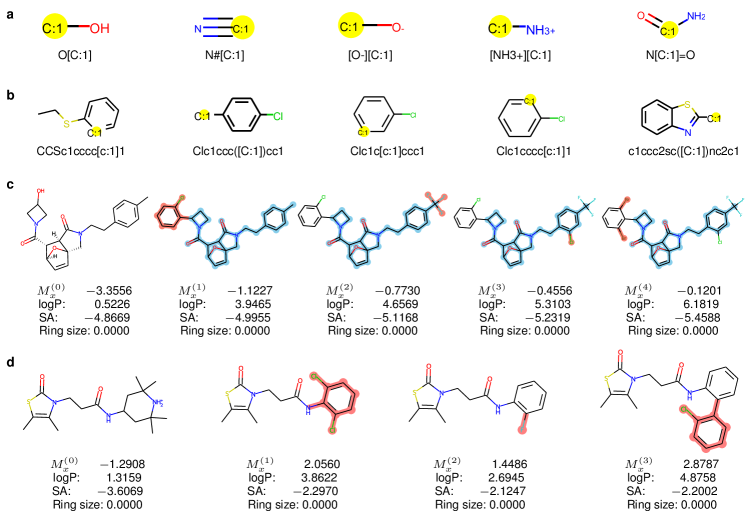
Among training molecules, the top-5 most popular fragments that have been removed from are presented in Fig. 1a with their canonical SMILE strings; the top-5 most popular fragments to be attached to generate are presented in Fig. 1b. Overall, the removal fragments in training data are on average of 2.85 atoms and the new attached fragments are of 7.55 atoms, that is, the optimization is typically done via removing small fragments and then attaching larger fragments.
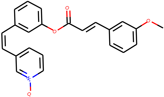
Fig. 1c presents an example of molecule (i.e., ) being optimized via four iterations in Modof-pipe into another molecule under =0.4. At each iteration, only one, small fragment (highlighted in red in the figure) is modified from its input, and pP value (below each molecule) is improved. In the first iteration, is modified from via the removal of the hydroxyl group in and the addition of the 2-chlorophenyl group. The hydroxyl group is polar and tends to increase water solubility of the molecules, while the 2-chlorophenyl group is non-polar and thus more hydrophobic. In addition, the increase in molecular weight brought by the chlorophenyl substituent would contribute to the lower water solubility as well. Thus, the modification from the hydroxyl group to the chlorophenyl group induces the P increase (from to ). Meanwhile, the introduction of the 2-chlorophenyl group to the cyclobutyl group adds complexity to the synthesis, in addition to possible steric effects due to the ortho-substitution on the aromatic ring, and induces a decrease in synthetic accessibility (SA) (from to ). In the second iteration, the methyl group in is replaced by a trifluoromethyl group. The trifluoromethyl group is more hydrophobic than the methyl group, and thus increases the P value of over (from to ). Meanwhile, the slightly larger molecule has slightly worse SA (from to ). If P is preferred to be lower than 5 as proposed in the Lipinski’s Rule of Five [31], Modof-pipe can be stopped at this iteration; otherwise, in the following two iterations, more halogens are added to the aromatic ring, which could make the aromatic ring less polar and further decrease water solubility and increase P values [32]. These four iterations highlight the interpretability of Modof-pipe corresponding to chemical knowledge. Please note that all the modifications in Modof are learned in an end-to-end fashion from data without any chemical rules or templates imposed a priori, emphasizing the power of Modof in learning from molecules.
In Fig. 1c, the molecule similarities between (=1,..,4) and are 0.630, 0.506, 0.421, 0.4111, respectively. This example also shows that Modof is able to retain the major scaffold of a molecule and optimizes at different disconnection sites during the iterative optimization process. Additional analysis on fragments is available in Section S10.
| Optimizing DRD2 | Optimizing QED | ||||||||||||||
| model | () | (imprv 0.2) | (0.9) | (imprv0.1) | |||||||||||
| rate% | imprvstd | simstd | rate% | imprvstd | simstd | rate% | imprvstd | simstd | rate% | imprvstd | simstd | ||||
| JTNN | 78.10 | 0.830.17 | 0.440.05 | 78.30 | 0.830.17 | 0.440.05 | 60.50 | 0.170.03 | 0.470.06 | 67.38 | 0.170.03 | 0.470.07 | |||
| HierG2G | 82.00 | 0.830.16 | 0.440.05 | 84.00 | 0.820.18 | 0.440.05 | 75.12 | 0.180.03 | 0.460.06 | 82.38 | 0.170.03 | 0.460.06 | |||
| JTNN(m) | 43.50 | 0.770.15 | 0.490.08 | 61.60 | 0.650.24 | 0.490.08 | 40.50 | 0.170.03 | 0.540.09 | 68.50 | 0.150.03 | 0.540.09 | |||
| HierG2G(m) | 51.80 | 0.780.15 | 0.490.08 | 70.20 | 0.660.24 | 0.490.08 | 37.12 | 0.170.03 | 0.520.09 | 65.88 | 0.150.03 | 0.530.10 | |||
| Modof-pipe | 74.90 | 0.830.14 | 0.480.07 | 89.00 | 0.750.22 | 0.480.07 | 40.00 | 0.170.03 | 0.510.08 | 70.00 | 0.160.03 | 0.510.08 | |||
| Modof-pipem | 88.60 | 0.880.12 | 0.460.05 | 95.90 | 0.840.18 | 0.460.05 | 66.25 | 0.180.03 | 0.480.07 | 87.62 | 0.170.03 | 0.480.07 | |||
-
•
Columns represent: : the optimized molecules that achieve a certain property improvement: (1) for DRD2, the optimized molecules should have DRD2 score no less than 0.5; (2) for QED, the optimized molecules should have QED score no less than 0.9. : the optimized molecules that achieve a property improvement in a similar degree as in training data: (1) for DRD2, the optimized molecules should satisfy ; (2) for QED, the optimized molecules should satisfy QED scores . “rate%”: the percentage of optimized molecules in each group (, , ) over all test molecules; “imprv”: the average property improvement; “std”: the standard deviation; “sim”: the similarity between the original molecules and optimized molecules . Best rate% values are in bold.
Performance on DRD2 and QED Optimization
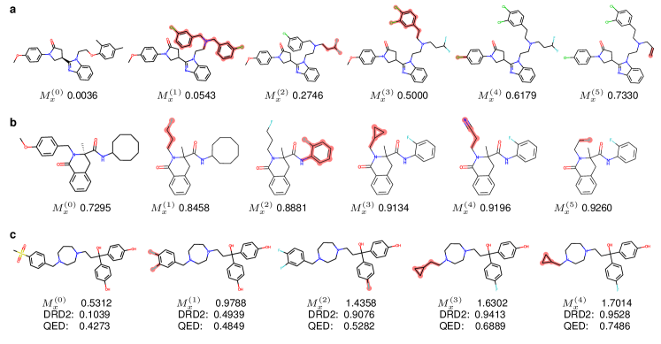
In addition to improving pP, another two popular benchmarking tasks for molecule optimization include improving molecule binding affinities against the dopamine D2 receptor (DRD2), and improving the drug-likeness estimated by quantitative measures (QED) [33]. Specifically, given a molecule that doesn’t bind well to the DRD2 receptor (e.g., with low binding affinities), the objective of optimizing DRD2 property is to modify the molecule into another one that will better bind to DRD2. In the QED task, given a molecule that is not much drug-like, the objective of optimizing QED property is to modify this molecule into a more “drug-like” molecule. Table 2 presents the major results in success rates, property improvement and similarity comparison under the similarity constraint =0.4. The results demonstrate that Modof-pipem significantly outperforms or is comparable to the baseline methods in optimizing DRD2 and QED, when the success rates are measured using either the benchmark metrics [14, 15] ( in Table 2) or based on training data ( in Table 2). Fig. 2a and Fig. 2b present two examples of molecule optimization for DRD2 and QED property improvement. Particularly, as in Fig. 2b, in the first iteration, a 4-methoxyphenyl group is removed and a small chain of 2-fluoroethyl group is added, and thus, the number of aromatic rings and the number of hydrogen bond acceptors are reduced, which makes the compound more drug-like than its predecessor. In the second iteration, a cyclooctyl group is removed from and a 2-fluorophenyl group is added. This modification may induce reduced flexibility – another preferred property of a successful drug. In the following iterations, some commonly used fragments in drug design are used to further modify the molecule into more drug-likeness. Note that, again, QED optimization is completely learned from data in an end-to-end fashion without any medicinal chemistry knowledge imposed by experts. The meaningful optimization in the example in Fig. 2b demonstrates the interpretability of Modof-pipe. More details about these two optimization tasks and results are available in the Section S11.
We also conducted experiments to optimize both DRD2 and QED properties of molecules simultaneously, that is, a multi-property optimization task. Details on this multi-property task and results are available in Section S12. Fig. 2c presents an example of multi-property molecule optimization, in which both the DRD2 and QED scores of the molecule are consistently increased with the iterations of optimization.
Discussions and Conclusions
Molecule Optimization using Simulated Properties
Most of the molecule properties considered in our experiments are based on simulated or predicted values rather than experimentally measured. That is, an independent simulation or machine learning model is first used to generate the property values for the benchmark dataset. For example, Crippen P is estimated via the Wildman and Crippen approach [21]; synthesis accessibility is calculated using a scoring function over predefined fragments [22]; the DRD2 property is predicted using a support vector machine classifier [34]; and the QED property is predicted using a non-linear classifier combining multiple desirability functions of molecular properties [33]. While all the existing generative models for molecule optimization [35, 9, 36, 8, 37, 14, 13, 15, 16, 19] use such simulated properties, there are both challenges and opportunities. Challenges arise when the simulation or machine learning models for those property predictions are not sufficiently accurate due to various reasons (e.g., limited or biased training molecules), the generative models learned from the inaccurate property values would also be inaccurate or incorrect, resulting in generated molecules that could negatively impact the downstream drug development tasks significantly. However, the opportunities due to the property simulation or prediction can be immense in fully unleashing the power of large-scale, data-driven learning paradigms to stimulate drug development as we continue to improve these simulations and predictions. Specifically, most deep learning-based models for drug development purposes, many of which have been demonstrated to be very promising [38], are not possible without large-scale training data. While it is impractical, if ever possible, to experimentally measure the interested properties for a large set of molecules (e.g., more than 100K molecules as in our benchmark training data), the property simulation or prediction of the molecules enables large training data and makes the development of such deep learning methodologies possible. Fortunately, property prediction simulations or models have become more accurate (e.g., 98% accuracy for DRD2 [34]) due to the accumulation of experimental measurements [39] and the strong learning power of innovative computational approaches. The accurate property simulation or prediction over large-scale molecule data and the powerful learning capability of generative models from such molecule data will together have strong potentials to further advance in silico drug development.
Synthesizability and Retrosynthesis
Our experiments show that Modof is also able to improve synthesis accessibility (Section S9.4). However, it does not necessarily mean that the generated molecules can be easily synthesized. This limitation of Modof is actually common for almost all the computational approaches for molecule generation. A recent study shows that many molecules generated via deep learning are not easily synthesizable [40], which significantly limits the translational potentials of the generative models in making real impacts in drug development. On the other hand, retrosynthesis prediction via deep learning, which aims to identify a feasible synthesis path for a given molecule through learning and searching from a large collection of synthesis paths, has been an active research area [41, 42]. Optimizing molecules towards not only better properties but also better synthesizability, particularly with explicit synthesis paths identified simultaneously, could be a highly interesting and challenging future research direction. Ultimately, we would like to develop a comprehensive computational framework that could generate synthesizable molecules with preferable properties. This would require not only a substantial amount of data to train sophisticated models, but also necessary domain knowledge and human experts looped in the learning process.
In vitro Validation
Testing the in silico generated molecules in a laboratory will be needed ultimately to validate the computational methods. While currently most existing computational methods are developed in academic environments and thus cannot be easily tested on purchasable or proprietary molecule libraries, or cannot be easily synthesized as we discussed earlier, a few successful stories [43] have demonstrated that powerful computational methods have high potentials to truly make new discoveries that can succeed in laboratory validation. Analogous to this molecule optimization and discovery process using deep learning approaches is from AlphaFold [44], a deep learning method predicting protein folding structures. The breakthrough from AlphaFold in solving a 50-year-old grand challenge in biology offers a strong evidence showing the tremendous power of modern learning approaches, which should not be underestimated. Still, collaborations with pharmaceutical industry and in vitro test are highly needed to truly translate the computational methods into real impact. In addition, effective sampling and/or prioritization of generated molecules in order to identify a feasible, small set of molecules for small-scale in vitro validation could be a practical solution; it will require the development of new sampling schemes over molecule subspaces, and/or the learning of molecule prioritization [45, 46] within the molecule generation process. Meanwhile, large-scale in vitro validation of in silico generated molecules represents a challenging but interesting future research direction.
Other Issues in Computational Molecule Optimization
A limitation of Modof-pipe is that it employs a local greedy optimization strategy: in each iteration, the input molecules to Modof will be optimized to the best, and if the optimized molecules do not have better properties, they will not go through additional Modof iterations. Detailed discussions on local greedy optimization are available in Section S13.1. In addition to partition coefficient, there are a lot of factors (e.g., toxicity, synthesizability) that need to be considered in order to develop a molecule into a drug. Discussions on multi-property optimization are available in Section S13.2. Target-specific molecule optimization are also discussed in Section S13.3. The Modof framework could also be used for compounds or substance property optimization in other application areas (e.g., melting or boiling points for volatiles). Related discussions are available in Section S13.4.
Conclusions
Modof optimizes molecules at one disconnection site at a time by learning the difference between molecules before and after optimization. With a much less complex model, it achieves significantly better or similar performance compared to the states of the art. In addition to the limitations and corresponding future research directions that have been discussed above, another limitation with Modof is that in Modof, the modification happens at the periphery of molecules. Although this is very common in in vitro lead optimization, we are currently investigating how Modof can be enhanced to modify the internal regions of molecules, if needed, by learning from proper training data with such regions. Additionally, we hope to integrate domain-specific knowledge in the Modof learning process facilitating increased explainability in the learning and generative process.
Methods
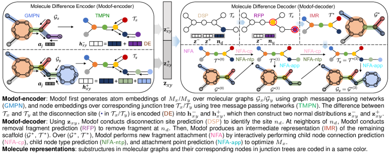
Modof modifies one fragment (e.g., a ring system, a linker, a side chain) of a molecule at a time, and thus only encodes and decodes the fragment that needs modification. The site of where the fragment is modified is referred to as the site of disconnection and denoted as , which corresponds to a node in the junction tree representation (discussed in ”Molecule Representations and Notations”). Fig. 3 presents an overview of Modof. All the algorithms are presented in Section S14. Discussions on the single-disconnection-site rationale are presented in Section S5.
Molecule Representations and Notations
We represent a molecule using a molecular graph and a junction tree . is denoted as , where is the set of atoms in , and is the set of corresponding bonds. In the junction tree representation [8], all the rings and bonds in are extracted as nodes in ; nodes with common atoms are connected with edges in . Thus, each node is a substructure (e.g., a ring, a bond and its connected atoms) in . We denote the atoms included in node as and refer to the nodes connected to in as its neighbors, denoted as . Thus, each edge actually corresponds to the common atoms between and . When no ambiguity arises, we will eliminate subscript in the notations. Note that atoms and bonds are the terms used for molecular graph representations, and nodes and edges are used for junction tree representations. In this manuscript, all the embedding vectors are by default column vectors, represented by lower-case bold letters; all the matrices are represented by upper-case letters. Key notations are listed in Table 3.
| notation | meaning |
|---|---|
| molecule represented by and | |
| molecular graph with atoms and bonds | |
| junction tree with nodes and edges | |
| an atom in | |
| a bond connecting atoms and in | |
| a node in | |
| an edge connecting nodes and in | |
| site of disconnection | |
| , | atoms included in a tree node , ’s neighbors |
| atom type embedding | |
| concatenation of , , … |
Molecular Difference Encoder (Modof-encoder)
Given two molecules , Modof (Algorithm S1 in Section S14) learns and encodes the difference between and using message passing networks [47] over graphs and , denoted as , and over junction trees and , denoted as , via three steps.
Step 1. Atom Embedding over Graphs ()
Modof first represents atoms using embeddings to capture atom types and their local neighborhood structures by propagating messages along bonds over molecular graphs. Modof uses an one-hot encoding to represent the type of atom , and an one-hot encoding to represent the type of bond connecting and . Each bond is associated with two messages and encoding the messages propagating from atom to and vice versa. The in -th iteration of is updated as follows:
where is initialized as zero, and ’s (=1,2,3) are the learnable parameter matrices. Thus, the message encodes the information of all length- paths passing through to in the graph. After iterations of message passing, the atom embedding is updated as follows:
where is the concatenation of message vectors from all iterations, and and are learnable parameter matrices. Thus, the atom embedding aggregates information from ’s -hop neighbors, similarly to Xu et al. [48], to improve the atom embedding representation power.
Step 2. Node Embedding over Junction Trees ()
Modof encodes nodes in junction trees into embeddings to capture their local neighborhood structures by passing messages along the tree edges. To produce rich representations of nodes, Modof first aggregates the information of atoms within a node into an embedding , and the information of atoms shared by a tree edge into an embedding through the following pooling:
| (1) |
| (2) |
Modof also uses a learnable embedding to represent the type of node . Thus, from node to in -th iteration of is updated as follows:
where is a concatenation of and so as to represent comprehensive node information, and ’s (=1,2, 3,4) are learnable parameter matrices. Similarly to the messages in , encodes the information of all length- paths passing through edge to in the tree. After iterations, the node embedding is updated as follows:
| (3) |
where ’s (=1,2,3) are the learnable parameter matrices.
Step 3. Difference Embedding ()
The difference embedding between and is calculated by pooling the node embeddings from and as follows:
where ’s/’s are the embeddings of nodes only appearing in and learned from / via . Note that in the above equations is the site of disconnection, and both and have the common node . Thus, essentially represents the fragment that should be removed from at and represents the fragment that should be attached to at afterwards in order to modify into . We will discuss how to identify , and the removed and new attached fragments at in and later in Section ”Molecular Difference Decoder (Modof-decoder)”.
As in VAE [49], we map the two difference embeddings and into two normal distributions by computing the mean and log variance with fully connected layers and . We then sample the latent vectors and from these two distributions and concatenate them into one latent vector , that is,
| (4) |
Thus, encodes the difference between and .
Molecular Difference Decoder (Modof-decoder)
Following the autoencoder idea, Modof decodes the difference embedding (Eqn 4) into edit operations that change into . Specifically, Modof first predicts a node in as the disconnection site. This node will split into several fragments, and the number of the resulted fragments depends on the number of ’s neighboring nodes . Modof then predicts which fragments to remove from , and merges the remaining fragments with into an intermediate representation . After that, Modof attaches new fragments sequentially starting from to . The decoding process (Algorithm S2 in Section S14) has the following 4 steps.
Step 1. Disconnection Site Prediction ()
Modof predicts a disconnection score for each ’s node as follows,
| (5) |
where is ’s embedding (Eqn 3) in , and ’s (=1,2) are learnable parameter vector and matrices, respectively. The node with the largest disconnection score is predicted as the disconnection site . Intuitively, Modof considers the neighboring or local structures of (in ) and “how likely” edit operations (represented by ) can be applied at . To learn , Modof uses the negative log likelihood of ground-truth disconnection site in tree as the loss function.
Step 2. Removal Fragment Prediction ()
Next, Modof predicts which fragments separated by should be removed from . For each node connected to , Modof predicts a removal score as follows,
| (6) |
where is sigmoid function, and ’s (=1,2) are learnable parameter vector and matrices, respectively. The fragment with a removal score greater than 0.5 is predicted to be removed. Thus, there could be multiple or no fragments removed. Intuitively, Modof considers the local structures of the fragment (i.e., ) and “how likely” this fragment should be removed (represented by ). To learn , Modof minimizes binary cross entropy loss to maximize the predicted scores of ground-truth removed fragments in .
Step 3. Intermediate Representation ()
After fragment removal, Modof merges the remaining fragments together with the disconnection site into an intermediate representation . may not be a valid molecule after some fragments are removed (some bonds are broken). It represents the scaffold of that should remain unchanged during the optimization. Modof first removes a fragment in order to identify such a scaffold and then adds a fragment to the scaffold to modify the molecule.
Step 4. New Fragment Attachment ()
Modof modifies into the optimized by attaching a new fragment (Algorithm S3 in Section S14). Modof uses the following four predictors to sequentially attach new nodes to . The predictors will be applied iteratively, starting from , on each newly attached node in . The attached new node in the -th step is denoted as (), and the corresponding molecular graph and tree are denoted as () and (), respectively.
Step 4.1. Child Connection Prediction () Modof first predicts whether should have a new child node attached to it, with the probability calculated as follows:
| (7) |
where is the embedding of node learned over (Eqn 3), (Eqn 4) indicates “how much” should be expanded, and and ’s (=1,2) are learnable parameter vector and matrices. If is above 0.5, Modof predicts that should have a new child node and thus child node type prediction will follow; otherwise, the optimization process stops at . To learn , Modof minimizes a binary cross entropy loss to maximize the probabilities of ground-truth child nodes. Note that may have multiple children, and therefore, once a child is generated as in the following steps and attached to , another child connection prediction will be conducted at with the updated embedding over the expanded . The above process will be iterated until is predicted to have no more children.
Step 4.2. Child Node Type Prediction () The new child node of is denoted as . Modof predicts the type of by calculating the probabilities of all types of the nodes that can be attached to as follows:
| (8) |
where converts a vector of values into probabilities, and ’s (=1,2) are learnable matrices. Modof assigns the new child the node type corresponding to the highest probability. Modof learns by minimizing cross entropy to maximize the likelihood of true child node types.
Step 4.3. Attachment Point Prediction () If node is predicted to have a child node , the next step is to connect and . If and share one or multiple atoms (e.g., and form a fused ring and thus share two adjacent atoms) that can be unambiguously determined as the attachment point(s) based on chemical rules, Modof will connect and via the atom(s). Otherwise, if and have multiple connection configurations, Modof predicts the attachment atoms at and , respectively.
Step 4.3.1. Attachment Point Prediction at Parent Node () Modof scores each candidate attachment point at parent node , denoted as , as follows,
| (9) |
where represents the embedding of ( could be an atom or a bond), is calculated by over ; is as in Eqn 3; is the sum of the embeddings of all atoms in (Eqn 1); and and (=1,2,3,4) are learnable vector and matrices. Modof intuitively measures “how likely” can be attached to by looking at its own (i.e., ), its context in (i.e., and neighbors ), its connecting node (i.e., ) and “how much” should be expanded (represented by ). The candidate with the highest score is selected as the attachment point in . Modof learns by minimizing the negative log likelihood of ground-truth attachment points.
Step 4.3.2. Attachment Point Prediction at Child Node () Modof scores each candidate attachment point at the child node , denoted as , as follows:
| (10) |
where represents the embedding of ( could be an atom or a bond) and is ’s embedding calculated over via ; and ’s (=1,2,3,4) are learnable parameters. Modof intuitively measures “how likely” candidate can be attached to at by looking at its own (i.e., ), the features of (i.e., ), its context in (i.e., ) and “how much” should be expanded (i.e., ). The candidate with the highest score is selected as the attachment point in . Modof learns by minimizing the negative log likelihood of ground-truth attachment points.
Valence Checking In , Modof incorporates valence check to only generate and predict legitimate candidate attachment points that do not violate valence laws.
Molecule size constraint Following You et al. [9], for pP optimization, we limit the size of optimized molecules to at most 38 (38 is the maximum number of atoms in the molecules in the ZINC dataset [23]). With this molecule size constraint, Modof can avoid increasing pP by trivially increasing molecule size, which may have the efforts of improving pP [50].
Sampling Schemes
In the decoding process, for each , Modof samples twenty times from the latent space of and optimize accordingly. Among all decoded molecules satisfying the similarity constraint with , Modof selects the one of best property as its output.
Modof Pipelines
A pipeline of Modof models, denoted as Modof-pipe (Algorithm S4 in Section S14), is constructed with a series of identical Modof models, with the output molecule from one Modof model as the input to the next. Given an input molecule to the -th Modof model (=), Modof first optimizes into as the output of this model. is then fed into the (+)-th model if it satisfies the similarity constraint and property constraint . Otherwise, is output as the final result and Modof-pipe stops. In addition to Modof-pipe, which outputs one optimized molecule for each input molecule, Modof-pipem is developed to output multiple optimized molecules for each input molecule. Details about Modof-pipem are available in Section S2.
The advantages of this iterative, one-fragment-at-one-time optimization process include that 1) it is easier to control intermediate optimization steps so as to result in optimized molecules of desired similarities and properties; 2) it is easier to optimize multiple fragments in a molecule that are far apart; and 3) it follows a rational molecule design process [11] and thus could enable more insights and inform in vitro lead optimization.
Model Training
During model training, we apply teacher forcing to feed the ground truth instead of the prediction results to the sequential decoding process. Following the idea of variational autoencoder, we minimize the following loss function to maximize the likelihood . Thus, the optimization problem is formulated as follows,
| (11) |
where is the set of parameters; is an estimated posterior probability function (Modof-encoder); is the probabilistic decoder representing the likelihood of generating given the latent embedding and ; and the prior follows . In the above problem, is the KL divergence between and . Specifically, the second term represents the prediction or empirical error, defined as the sum of all the loss functions in the above six predictions (Eqn 5-10). We use AMSGRAD [51] to optimize the learning objective.
Data Availability
The data used in this manuscript is made publicly available at Chen et al. [52] and the link https://github.com/ziqi92/Modof.
Code Availability
The code for Modof, Modof-pipe and Modof-pipem is made publicly available at Chen et al. [52] and
the link
https://github.com/ziqi92/Modof.
Acknowledgements
This project was made possible, in part, by support from the National Science Foundation grant numbers (IIS-1855501, X.N.; IIS-1827472, X.N.; IIS-2133650, X.N., S.P.; OAC-2018627, S.P.), and the National Library of Medicine (grant numbers 1R01LM012605-01A1, X.N.; and 1R21LM013678-01, X.N.), an AWS Machine Learning Research Award (X.N.) and The Ohio State University President’s Research Excellence program (X.N.). Any opinions, findings, and conclusions or recommendations expressed in this material are those of the authors, and do not necessarily reflect the views of the funding agencies. We thank Dr. Xiaoxue Wang and Dr. Xiaolin Cheng for their constructive comments.
Author Contributions
X.N. conceived the research; X.N. and S.P. obtained funding for the research, and co-supervised Z.C.; Z.C., M.R.M., S.P. and X.N. designed the research; Z.C. and X.N. conducted the research, including data curation, formal analysis, methodology design and implementation, result analysis and visualization; Z.C. drafted the original manuscript; M.R.M. provided comments on the original manuscript; Z.C., X.N. and S.P. conducted the manuscript editing and revision; all authors reviewed the final manuscript.
Competing Interests
M.R.M. was employed by the company NEC Labs America. The remaining authors declare that the research was conducted in the absence of any commercial or financial relationships that could be construed as a potential conflict of interest.
References
- 1. Jorgensen, W. L. Efficient drug lead discovery and optimization. Acc. Chem. Res. 42, 724–733 (2009).
- 2. Verdonk, M. L. & Hartshorn, M. J. Structure-guided fragment screening for lead discovery. Curr. Opin. Drug Discov. Devel. 7, 404 (2004).
- 3. de Souza Neto, L. R. et al. In silico strategies to support fragment-to-lead optimization in drug discovery. Front. Chem. 8 (2020).
- 4. Hoffer, L. et al. Integrated strategy for lead optimization based on fragment growing: the diversity-oriented-target-focused-synthesis approach. J. Med. Chem. 61, 5719–5732 (2018).
- 5. Gerry, C. J. & Schreiber, S. L. Chemical probes and drug leads from advances in synthetic planning and methodology. Nat. Rev. Drug Discov. 17, 333 (2018).
- 6. Sattarov, B. et al. De novo molecular design by combining deep autoencoder recurrent neural networks with generative topographic mapping. J. Chem. Inf. Model. 59, 1182–1196 (2019).
- 7. Sanchez-Lengeling, B. & Aspuru-Guzik, A. Inverse molecular design using machine learning: Generative models for matter engineering. Science 361, 360–365 (2018).
- 8. Jin, W., Barzilay, R. & Jaakkola, T. Junction tree variational autoencoder for molecular graph generation. vol. 80 of Proceedings of Machine Learning Research, 2323–2332 (Stockholmsmässan, Stockholm Sweden, 2018).
- 9. You, J., Liu, B., Ying, Z., Pande, V. & Leskovec, J. Graph convolutional policy network for goal-directed molecular graph generation. In Bengio, S. et al. (eds.) Advances in Neural Information Processing Systems 31, 6410–6421 (2018).
- 10. Murray, C. & Rees, D. The rise of fragment-based drug discovery. Nat. Chem. 1, 187–92 (2009).
- 11. Hajduk, P. J. & Greer, J. A decade of fragment-based drug design: strategic advances and lessons learned. Nat. Rev. Drug Discov. 6, 211–219 (2007).
- 12. Shi, C. et al. Graphaf: a flow-based autoregressive model for molecular graph generation. In 8th International Conference on Learning Representations, Addis Ababa, Ethiopia, April 26-30, 2020 (2020).
- 13. Zang, C. & Wang, F. Moflow: An invertible flow model for generating molecular graphs. In Gupta, R., Liu, Y., Tang, J. & Prakash, B. A. (eds.) KDD ’20: The 26th ACM SIGKDD Conference on Knowledge Discovery and Data Mining, Virtual Event, CA, USA, August 23-27, 2020, 617–626 (2020).
- 14. Jin, W., Yang, K., Barzilay, R. & Jaakkola, T. S. Learning multimodal graph-to-graph translation for molecule optimization. In 7th International Conference on Learning Representations, New Orleans, LA, USA, May 6-9, 2019 (2019).
- 15. Jin, W., Barzilay, R. & Jaakkola, T. S. Hierarchical generation of molecular graphs using structural motifs. In Proceedings of the 37th International Conference on Machine Learning, 13-18 July 2020, Virtual Event, vol. 119 of Proceedings of Machine Learning Research, 4839–4848 (2020).
- 16. Podda, M., Bacciu, D. & Micheli, A. A deep generative model for fragment-based molecule generation. In Chiappa, S. & Calandra, R. (eds.) Proceedings of the Twenty Third International Conference on Artificial Intelligence and Statistics, vol. 108 of Proceedings of Machine Learning Research, 2240–2250 (2020).
- 17. Ji, C., Zheng, Y., Wang, R., Cai, Y. & Wu, H. Graph polish: A novel graph generation paradigm for molecular optimization. CoRR abs/2008.06246 (2020). 2008.06246.
- 18. Lim, J., Hwang, S.-Y., Moon, S., Kim, S. & Kim, W. Y. Scaffold-based molecular design with a graph generative model. Chem. Sci. 11, 1153–1164 (2020).
- 19. Ahn, S., Kim, J., Lee, H. & Shin, J. Guiding deep molecular optimization with genetic exploration. In Larochelle, H., Ranzato, M., Hadsell, R., Balcan, M. & Lin, H. (eds.) Advances in Neural Information Processing Systems 33: Annual Conference on Neural Information Processing Systems 2020, December 6-12, 2020, virtual (2020).
- 20. Nigam, A., Friederich, P., Krenn, M. & Aspuru-Guzik, A. Augmenting genetic algorithms with deep neural networks for exploring the chemical space. In 8th International Conference on Learning Representations, Addis Ababa, Ethiopia, April 26-30, 2020 (2020).
- 21. Wildman, S. A. & Crippen, G. M. Prediction of physicochemical parameters by atomic contributions. J. Chem. Inf. Comput. Sci. 39, 868–873 (1999).
- 22. Ertl, P. & Schuffenhauer, A. Estimation of synthetic accessibility score of drug-like molecules based on molecular complexity and fragment contributions. J. Cheminf. 1, 8 (2009).
- 23. Sterling, T. & Irwin, J. J. Zinc 15–ligand discovery for everyone. J. Chem. Inf. Model. 55, 2324–2337 (2015).
- 24. Gómez-Bombarelli, R. et al. Automatic chemical design using a data-driven continuous representation of molecules. ACS Cent. Sci. 4, 268–276 (2018).
- 25. Abu-Aisheh, Z., Raveaux, R., Ramel, J.-Y. & Martineau, P. An exact graph edit distance algorithm for solving pattern recognition problems. In Proceedings of the International Conference on Pattern Recognition Applications and Methods - Volume 1, 271–278 (Setubal, PRT, 2015).
- 26. Sanfeliu, A. & Fu, K. A distance measure between attributed relational graphs for pattern recognition. IEEE Trans. Syst. Man Cybern. SMC-13, 353–362 (1983).
- 27. Lipinski, C. A. Lead-and drug-like compounds: the rule-of-five revolution. Drug Discov. Today Technol. 1, 337–341 (2004).
- 28. Ghose, A. K., Viswanadhan, V. N. & Wendoloski, J. J. A knowledge-based approach in designing combinatorial or medicinal chemistry libraries for drug discovery. 1. a qualitative and quantitative characterization of known drug databases. J. Comb. Chem. 1, 55–68 (1999).
- 29. Whiteson, S., Tanner, B., Taylor, M. E. & Stone, P. Protecting against evaluation overfitting in empirical reinforcement learning. In 2011 IEEE Symposium on Adaptive Dynamic Programming and Reinforcement Learning, 120–127 (2011).
- 30. Zhang, C., Vinyals, O., Munos, R. & Bengio, S. A study on overfitting in deep reinforcement learning. CoRR abs/1804.06893 (2018). 1804.06893.
- 31. Lipinski, C. A., Lombardo, F., Dominy, B. W. & Feeney, P. J. Experimental and computational approaches to estimate solubility and permeability in drug discovery and development settings. Adv. Drug Deliv. Rev. 46, 3–26 (2001).
- 32. Rokitskaya, T. I., Luzhkov, V. B., Korshunova, G. A., Tashlitsky, V. N. & Antonenko, Y. N. Effect of methyl and halogen substituents on the transmembrane movement of lipophilic ions. Phys. Chem. Chem. Phys. 21, 23355–23363 (2019).
- 33. Bickerton, G. R., Paolini, G. V., Besnard, J., Muresan, S. & Hopkins, A. L. Quantifying the chemical beauty of drugs. Nat. Chem. 4, 90–98 (2012).
- 34. Olivecrona, M., Blaschke, T., Engkvist, O. & Chen, H. Molecular de-novo design through deep reinforcement learning. J. Cheminf. 9 (2017).
- 35. Kusner, M. J., Paige, B. & Hernández-Lobato, J. M. Grammar variational autoencoder. In Precup, D. & Teh, Y. W. (eds.) Proceedings of the 34th International Conference on Machine Learning, Sydney, NSW, Australia, 6-11 August 2017, vol. 70 of Proceedings of Machine Learning Research, 1945–1954 (2017).
- 36. De Cao, N. & Kipf, T. MolGAN: An implicit generative model for small molecular graphs. ICML 2018 workshop on Theoretical Foundations and Applications of Deep Generative Models (2018).
- 37. Zhou, Z., Kearnes, S., Li, L., Zare, R. N. & Riley, P. Optimization of molecules via deep reinforcement learning. Sci. Rep. 9, 1–10 (2019).
- 38. Wainberg, M., Merico, D., Delong, A. & Frey, B. J. Deep learning in biomedicine. Nat. Biotechnol. 36, 829–838 (2018).
- 39. Kim, S. et al. PubChem in 2021: new data content and improved web interfaces. Nucleic Acids Res. 49, D1388–D1395 (2020).
- 40. Gao, W. & Coley, C. W. The synthesizability of molecules proposed by generative models. J. Chem. Inf. Model. (2020).
- 41. Segler, M. H. S., Preuss, M. & Waller, M. P. Planning chemical syntheses with deep neural networks and symbolic AI. Nature 555, 604–610 (2018).
- 42. Kishimoto, A., Buesser, B., Chen, B. & Botea, A. Depth-first proof-number search with heuristic edge cost and application to chemical synthesis planning. In Wallach, H. M. et al. (eds.) Advances in Neural Information Processing Systems 32: Annual Conference on Neural Information Processing Systems 2019, December 8-14, 2019, Vancouver, BC, Canada, 7224–7234 (2019).
- 43. Stokes, J. M. et al. A deep learning approach to antibiotic discovery. Cell 180, 688–702.e13 (2020).
- 44. Liu, J. & Ning, X. Multi-assay-based compound prioritization via assistance utilization: A machine learning framework. J. Chem. Inf. Model. 57, 484–498 (2017).
- 45. Liu, J. & Ning, X. Differential compound prioritization via bidirectional selectivity push with power. J. Chem. Inf. Model. 57, 2958–2975 (2017).
- 46. Gilmer, J., Schoenholz, S. S., Riley, P. F., Vinyals, O. & Dahl, G. E. Neural message passing for quantum chemistry. In Proceedings of the 34th International Conference on Machine Learning - Volume 70, 1263–1272 (2017).
- 47. Xu, K., Hu, W., Leskovec, J. & Jegelka, S. How powerful are graph neural networks? In 7th International Conference on Learning Representations, New Orleans, LA, USA, May 6-9, 2019 (2019).
- 48. Kingma, D. P. & Welling, M. Auto-encoding variational bayes. In Bengio, Y. & LeCun, Y. (eds.) 2nd International Conference on Learning Representations, Banff, AB, Canada, April 14-16, 2014, Conference Track Proceedings (2014).
- 49. Wildman, S. A. & Crippen, G. M. Prediction of physicochemical parameters by atomic contributions. J. Chem. Inf. Comput. Sci. 39, 868–873 (1999).
- 50. Reddi, S. J., Kale, S. & Kumar, S. On the convergence of adam and beyond. In 6th International Conference on Learning Representations, Vancouver, BC, Canada, April 30 - May 3, 2018, Conference Track Proceedings (2018).
- 51. Chen, Z. A deep generative model for molecule optimization via one fragment modification. http://doi.org/10.5281/zenodo.4667928 (2021).
A Deep Generative Model for Molecule Optimization via One Fragment Modification (Supplementary Information)
Additional Related Work
There exists some limited work that follow the fragment-based drug design as Modof does. Podda et al. [16] decomposed molecules into fragments using an algorithm that breaks bonds according to chemical reactions. They then represented each fragment using its SMILES string and generated molecules via a VAE-based model, which sequentially decodes the SMILES strings of the fragments and reassembles the decoded SMILES strings into complete molecules.
Similar to Modof, a recent work named Teacher and Student polish (T&S polish) [17] also proposed to retain the scaffolds and edit the molecules by removing and adding fragments. However, Modof is fundamentally different from T&S polish. T&S polish employs a teacher component to identify the logic rules from training molecules that can transform one molecule to another with better properties. Thus, the logic rules describe an one-to-one mapping between the two molecules. T&S polish then learns from these logic rules in the student component, and uses the student component to polish or modify new molecules. The limitation of T&S polish is that it generates only one modified molecule for each input molecule. However, there could be multiple ways to optimize one molecule, and as suggested in Jin et al. [14], generative models should be able to generate such multiple, diverse optimized molecules for each input molecule. In contrast to T&S polish, Modof samples from a latent ‘difference’ distribution during testing and thus is able to generate multiple diverse optimized molecules.
In addition to T&S polish, Lim et al. [18] also developed a scaffold-based method to generate the molecules from scaffolds. Their method takes a scaffold as input and completes the input scaffold into a molecule through sequentially adding atoms and bonds via a VAE-based model. The limitation of their method is that the retained scaffolds must be cyclic skeletons extracted from training data by removing side-chain atoms. Due to this pre-defined scaffold vocabulary, their model is only able to add side-chain atoms to input scaffolds, and their generated molecules are limited within the chemical subspace shattered by their scaffold vocabulary. In contrast to their method, Modof is able to learn to determine the scaffolds that need to be retained from input test molecules, and completes the identified scaffolds with fragments that could be more complicated than just side-chain atoms. Hence, Modof has the potential to explore more widely in the chemical space for molecule optimization. We could not compare Modof with T&S polish as the T&S polish authors haven’t published their code. They also applied a different experimental setting (e.g., sample only once for all the baseline methods and thus lead to underestimation of the baselines) so that we could not directly use their reported results. Issues related to their parameter setting are discussed in Supplementary Information Section S6.
In addition to deep generative models, some genetic algorithm-based methods are also developed to find molecules with better properties. Ahn et al. [19] developed a genetic expert-guided learning method (GEGL), in which they used an expert policy to modify molecules through mutation and crossover, and learned a parameterized apprentice policy from good molecules modified by the expert policy for imitation learning. Nigam et al. [20] used a genetic algorithm to modify molecules with random mutations defined in Krenn et al. [53], and employed a discriminator to prevent the genetic algorithm from searching the same or similar molecules repeatedly.
Modof-pipem Protocol
We further allow Modof-pipe to output multiple, diverse optimized molecules (the corresponding pipeline denoted as Modof-pipem) following the below protocol:
-
1)
At the -th iteration in Modof-pipem, Modof optimizes each input molecule into 20 output molecules via 20 times of sampling and decoding.
-
2)
Among all the output molecules from iteration that satisfy the similarity constraint, the top-5 molecules with the best properties are fed into the next, (+1)-th iteration. The remaining output molecules may still have better properties compared to the input molecule to Modof-pipem, but they will not be further optimized by Modof-pipem. Note that the top-5 molecules may not always have improved properties (e.g., when all the output molecules do not have improved properties), but they will still be further optimized in the downstream iterations.
-
3)
The above two steps are conducted at each iteration up to five iterations, or until the iteration does not output any molecules (e.g., molecules cannot be decoded, similarity constraints are not satisfied), and then Modof-pipem stops.
-
4)
Once Modof-pipem has stopped, all the unique molecules output at each iteration that are not further optimized (either not fed into the next iteration, or output at the last iteration) are collected, and the top-20 molecules among them with the best properties will be the output, optimized molecules of Modof-pipem.
Algorithm S5 presents the Modof-pipem algorithm.
Data Used in pP Optimization Experiments
| description | value |
| #training molecules | 104,708 |
| #training (, ) pairs | 55,686 |
| #validation molecules | 200 |
| #test molecules | 800 |
| average similarity of training (, ) pairs | 0.6654 |
| average pairwise similarity between training and test molecules | 0.1070 |
| average training molecule size | 25.04 |
| average training size | 22.75 |
| average training size | 27.07 |
| average test molecule size | 20.50 |
| average pP | -0.7362 |
| average pP | 1.1638 |
| average test molecule pP | -2.7468 |
| average pP improvement in training (, ) pairs | 1.9000 |
Table S1 presents the statistics of the data used in our experiments for pP optimization.
Training Data Representativeness
The training data used in our experiments and the baseline methods are extracted from the widely used ZINC dataset. The ZINC dataset is relatively standard for problems including chemical property prediction [54], chemical synthesis [55], optimization [14, 15], etc. Instead of using the entire ZINC or a random subset of ZINC, in Modof, we used pairs of molecules in ZINC that satisfy a particular structural constraint: the molecules in a pair are only different in structures at one disconnection site. Whether Modof’s training data well represent the ZINC chemical space will affect whether Modof can be well generalized in the entire ZINC space.
To analyze the representativeness of Modof’s training data, we conducted the following analysis: We clustered the following three groups of molecules all together: (1) the molecules in Modof’s training pairs that have bad properties, denoted as ; (2) the molecules in Modof’s training pairs that have good properties, denoted as ; and (3) the rest, all the ZINC molecules that are not in and , denoted as . In total, we had 324,949 molecules to cluster. We first represented each molecule using its canonical SMILE string, and generated a 2,048-dimension binary Morgan fingerprint based on the SMILE string. We then clustered the 324,949 molecules using the CLUTO [56] clustering software. CLUTO constructs a graph among the molecules, in which each molecule is connected to its nearest neighbors defined by molecule similarities calculated via Tanimoto coefficient over molecule fingerprints. Please note that this is exactly the same molecule similarity calculation used in Modof.
Fig. S1 presents the results from 56 clusters (50 clusters and 6 disconnected components in the nearest-neighbor graphs). In Fig. S1, the clusters are sorted based on their size, and the axis represents the percentage of molecules in , training data (i.e., ), or that fall within in each cluster. Fig. S1 shows that Modof’s training data, and have data distributions similar to ZINC data in each of the clusters. We also conducted six paired -tests over the data distributions among all the group pairs between , , and . The -tests show no statistically significant difference in data distributions over clusters among the four groups of molecules, with all the -values close to 1.0. This indicates that Modof’s training data actually well represent the entire ZINC data, and thus Modof is generalizable and applicable to ZINC molecules outside Modof’s training data. We also tried different numbers of clusters (e.g., 100, 200), and the above conclusions remain the same.
Graph Edit Path Identification for Training Data Generation
Graph edit distance between tree and is defined as the minimum cost to modify into with the following graph edit operations:
-
•
Node addition: add a new labeled node into ;
-
•
Node deletion: delete an existing node from ;
-
•
Edge addition: add a new edge between a pair of nodes in ; and
-
•
Edge deletion: delete an existing edge between a pair of nodes in .
Particularly, we did not allow node or edge substitutions as they can be implemented via deletion and addition operations. We identified the optimal graph edit paths using the DF-GED algorithm [25] provided by a widely-used package NetworkX [57]. To identify disconnection sites, we denoted the common nodes between and as matched nodes (i.e., = ), nodes only in as the removal nodes (i.e., = ), and the nodes only in as the new nodes (i.e., = ), all with respect to . Therefore, the disconnection sites will be the matched nodes in that are also connected with a new node or a removal node, that is, .
Disconnection Site Analysis in pP Training Data
The key idea of Modof is to modify one fragment at a time under the similarity and property constraints. This is based on the assumption that for a pair of molecules with a high similarity (e.g., ), they are very likely to have only one (small) fragment different, and thus one site of disconnection. Fig. 2(a) presents the number of disconnection sites among the 75K pairs of molecules in the benchmark dataset provided by Jin et al. [15], in which each pair has similarity above 0.6. The distribution in Fig. 2(a) shows that when the molecule similarity is high (e.g., 0.6 in the benchmark dataset), most of the molecule pairs (i.e., 74.4%) have only one disconnection site, some of the pairs have two (i.e., 21.1%), and only a few have three. This indicates that one-fragment modification at a time is a rational idea and directly applicable to the majority of the optimization cases. Even though there could be more disconnection sites, Modof-pipe and Modof-pipem allow multiple-fragment optimization via multiple one-fragment optimizations.
Fig. 2(b) presents the number of nodes (as in junction tree representations) that need to be removed from the disconnection sites at (), and the number of nodes that need to be attached at the sites afterwards, in Jin’s benchmark dataset [15]. The figures show that on average, more nodes will be attached to the disconnection sites compared to the removal nodes. This indicates that the optimized molecules with better pP will become larger, as we have observed in our and other’s methods.
Discussion on Parameter Settings in pP Optimization
Among all the methods that involve random sampling, JTNN, HierG2G and our method Modof sample 20 times for each test molecule and thus produce 20 optimized candidates, and identify the best one among these 20 candidates. However, GraphAF optimized each test molecule for 200 times and reported the best among those 200 candidates. Thus, it is unclear if the overall performance of GraphAF is largely due to the many times of optimization (and thus a larger pool of optimized candidates) or the model that does learn how to optimize. T&S polish [17] forced all their compared baseline models including JTNN and GCPN to sample only once for each test molecule, because T&S polish can only modify one input molecule into one output. This might not be appropriate either since it artificially underestimated the performance of the baseline models. Instead, it would be fair to compare the output from T&S polish with the best output from the baseline methods.
Molecule Similarity Calculation
All baselines except JT-VAE in Table 1 in the main manuscript use binary Morgan fingerprints with radius of 2 and 2,048 bits to represent the presence or absence of particular, pre-defined substructures in molecules. Using such binary fingerprints in molecule similarity calculation may overestimate molecule similarities. An example is presented in Fig. S3, where the Tanimoto similarity from binary Morgan fingerprints () of the two molecules is 0.644, but they look sufficiently different, with the similarity from Morgan fingerprints of substructure counts () only 0.393. According to our experimental results (e.g., Fig. 1c and Fig. 1d in the main manuscript) and fragment analysis later in Section S10, we observed that aromatic rings could contribute to large pP values and thus would be attached to the optimized molecules. Using binary Morgan fingerprints in calculating molecule similarities in this case would easily lead to the solution that many aromatic rings will be attached for molecule optimization, while still satisfying the similarity constraint due to the similarity overestimation, but result in very large molecules that are less drug-like [28]. Therefore, to prevent the model from generating such molecules, we could either consider Morgan fingerprints of substructure counts, or limit the size of optimized molecules. In Modof, we used the same binary Morgan fingerprints as in the baselines and added an additional constraint to limit the size of optimized molecules to be at most 38 (38 is the maximum number of atoms in the molecules in the ZINC dataset).
=0.644,
=0.393
| #in% | #p% | #n% | #z% | property improvement | molecule sim | avgsim w. Trn | top sim w. Trn | simt | ||||||||||
|---|---|---|---|---|---|---|---|---|---|---|---|---|---|---|---|---|---|---|
| ptstd | ntstd | pstd | simtstd | simstd | all | Trnx | Trny | all | Trnx | Trny | ||||||||
| 0.0 | 1 | 100.00 | 99.62 | 0.00 | 0.38 | 5.121.73 | 0.000.00 | 5.101.76 | 0.430.13 | 0.440.13 | 0.119 | 0.112 | 0.125 | 0.369 | 0.333 | 0.355 | 0.146 | |
| 2 | 99.62 | 84.88 | 0.62 | 14.12 | 1.941.26 | -1.551.12 | 6.742.14 | 0.630.19 | 0.260.15 | 0.116 | 0.107 | 0.125 | 0.365 | 0.319 | 0.358 | 0.173 | ||
| 3 | 84.88 | 55.00 | 1.75 | 28.12 | 1.070.98 | -0.520.59 | 7.332.23 | 0.760.21 | 0.220.15 | 0.114 | 0.103 | 0.124 | 0.365 | 0.312 | 0.360 | 0.194 | ||
| 4 | 55.75 | 32.12 | 0.38 | 23.25 | 0.620.76 | -0.600.78 | 7.532.28 | 0.840.18 | 0.220.15 | 0.111 | 0.099 | 0.122 | 0.361 | 0.306 | 0.358 | 0.213 | ||
| 5 | 32.50 | 16.50 | 0.38 | 15.62 | 0.490.61 | -1.681.98 | 7.612.30 | 0.860.17 | 0.210.15 | 0.107 | 0.095 | 0.119 | 0.356 | 0.299 | 0.353 | 0.225 | ||
| 0.2 | 1 | 100.00 | 99.62 | 0.00 | 0.38 | 4.921.58 | 0.000.00 | 4.911.60 | 0.460.13 | 0.460.12 | 0.117 | 0.111 | 0.123 | 0.364 | 0.334 | 0.346 | 0.138 | |
| 2 | 99.62 | 68.75 | 2.38 | 28.50 | 1.540.97 | -0.780.84 | 5.971.73 | 0.710.19 | 0.360.11 | 0.117 | 0.109 | 0.125 | 0.351 | 0.317 | 0.340 | 0.154 | ||
| 3 | 70.12 | 28.62 | 3.25 | 38.25 | 0.750.71 | -0.670.87 | 6.181.76 | 0.860.15 | 0.340.11 | 0.117 | 0.108 | 0.125 | 0.348 | 0.312 | 0.340 | 0.166 | ||
| 4 | 29.88 | 8.38 | 1.25 | 20.25 | 0.530.48 | -0.280.28 | 6.221.77 | 0.920.13 | 0.340.11 | 0.115 | 0.106 | 0.124 | 0.345 | 0.307 | 0.338 | 0.175 | ||
| 5 | 9.25 | 1.75 | 0.25 | 7.25 | 0.320.22 | -0.170.14 | 6.231.77 | 0.960.09 | 0.340.11 | 0.113 | 0.103 | 0.122 | 0.344 | 0.308 | 0.338 | 0.177 | ||
| 0.4 | 1 | 100.00 | 99.12 | 0.00 | 0.88 | 4.501.32 | 0.000.00 | 4.471.38 | 0.530.11 | 0.530.11 | 0.114 | 0.110 | 0.118 | 0.366 | 0.338 | 0.344 | 0.131 | |
| 2 | 99.12 | 34.25 | 3.00 | 61.88 | 1.360.95 | -0.650.56 | 4.931.49 | 0.750.22 | 0.490.09 | 0.114 | 0.110 | 0.119 | 0.360 | 0.331 | 0.341 | 0.134 | ||
| 3 | 37.62 | 8.62 | 0.75 | 28.25 | 0.650.64 | -0.770.67 | 4.991.52 | 0.910.14 | 0.480.09 | 0.115 | 0.110 | 0.120 | 0.360 | 0.329 | 0.343 | 0.146 | ||
| 4 | 9.25 | 1.88 | 0.12 | 7.25 | 0.570.54 | -0.290.00 | 5.001.53 | 0.930.12 | 0.480.09 | 0.114 | 0.109 | 0.119 | 0.358 | 0.328 | 0.341 | 0.149 | ||
| 5 | 2.25 | 0.38 | 0.00 | 1.88 | 0.370.06 | 0.000.00 | 5.001.53 | 0.970.06 | 0.480.09 | 0.112 | 0.107 | 0.117 | 0.355 | 0.328 | 0.335 | 0.142 | ||
| 0.6 | 1 | 100.00 | 84.25 | 0.12 | 15.62 | 3.011.16 | -0.310.00 | 2.541.53 | 0.600.23 | 0.660.05 | 0.109 | 0.107 | 0.111 | 0.383 | 0.360 | 0.351 | 0.117 | |
| 2 | 84.25 | 14.62 | 1.88 | 67.75 | 1.160.92 | -0.690.76 | 2.711.68 | 0.830.17 | 0.660.05 | 0.113 | 0.111 | 0.116 | 0.382 | 0.357 | 0.355 | 0.128 | ||
| 3 | 16.00 | 1.00 | 0.25 | 14.75 | 0.840.67 | -0.030.00 | 2.721.68 | 0.940.11 | 0.650.05 | 0.113 | 0.109 | 0.117 | 0.369 | 0.342 | 0.346 | 0.136 | ||
| 4 | 1.25 | 0.12 | 0.00 | 1.12 | 0.380.00 | 0.000.00 | 2.721.68 | 0.920.14 | 0.650.05 | 0.117 | 0.112 | 0.121 | 0.351 | 0.322 | 0.334 | 0.147 | ||
| 5 | 0.12 | 0.00 | 0.00 | 0.12 | 0.000.00 | 0.000.00 | 2.721.68 | 0.000.00 | 0.650.05 | 0.111 | 0.107 | 0.115 | 0.271 | 0.255 | 0.262 | 0.000 | ||
-
•
Columns represent: “”: the iteration; ‘#in%”: the number of input molecules in each iteration in percentage over all the testing molecules; “#p”/“#n”/“#z%”: the percentage of molecules optimized with better/worse/same properties; “pt”/“nt”: property improvement/decline in the -th iteration; “p”: the overall property improvement up to the -th iteration; “simt”/“sim”: the similarities between the molecules before and after optimization in/up to the -th iteration; “avgsim w. Trn”/“top-10 sim w. Trn”: the average similarities with all/top-10 most similar training molecules; “all”/“Trnx”/‘Trny”: the comparison molecules identified from all/poor-property/good-property training molecules; “simt ”: the average pairwise similarities among optimized molecules.
Comparison Fairness among Existing Methods
Discussion on pP Test Sets
Note that in Table 1 in the main manuscript, the results of GraphAF and MoFlow are lower than those reported in the respective paper. This is because in their papers, they used a different test set rather than the benchmark test set, and their test molecules were much easier to optimize, which would lead to an unfair comparison with other baseline methods. In our experiments, we tested GraphAF and MoFlow on the benchmark test set and reported the results in Table 1 in the main manuscript.
The benchmark test set consists of 800 molecules that have the lowest pP values in ZINC test set (ZINC test set was split by Gómez-Bombarelli et al. [24]). The pP values of these molecules are in range [-11.02, -0.56], with an average value -2.751.52. The test set used in GraphAF and MoFlow consists of 800 molecules that have the lowest pP values from the entire ZINC dataset, not only from the ZINC test set. The pP values of these molecules are in range [-62.52, 2.42], with an average score -12.005.89. That is, the GraphAF and MoFlow’s test molecules have much worse properties compared to those in the benchmark test set, and they are much easier to optimize with larger property improvement. Due to the different test sets, the results reported in GraphAF and MoFlow are not comparable to those reported in other baseline methods.
For GraphAF, we fine-tuned their pre-trained model with a set of 10K molecules that do not overlap with the benchmark test set. We tested MoFlow using the trained model provided by its authors (note that MoFlow training learns molecule latent representations, not how to optimize molecules; molecule optimization is conducted during testing via gradient-ascent search in the latent representation space). The results show that unfortunately, GraphAF and MoFlow do not outperform GCPN, JTNN, HierG2G and our method Modof on the benchmark test data.
Discussion on Reinforcement Learning Settings
GCPN, MolDQN and GraphAF are reinforcement learning-based methods. They all used the 800 test molecules (benchmark test set for GCPN and MolDQN, and a different non-benchmark test set for GraphAF) to either directly train a model or fine-tune a pre-trained model to optimize the test molecules. Therefore, these models are specific to their test set, and would suffer from overfitting issues and not generalize to new molecules. They may also have the issue of not really learning but essentially memorizing optimization actions/paths. Previous studies have analyzed this so-called environment overfitting problem [29, 30] in reinforcement learning. They concluded that using a test set with overlapping samples in the training set (i.e., non-isolated test set) can lead to artificially high performance by simply memorizing the sequences of actions, and suggested that reinforcement learning should use an isolated test set that is completely disjoint with training set. The issues with non-isolated test sets remain true for GCPN, MolDQN and GraphAF.
In our experiments on GraphAF, instead of using the test set to fine-tune the pre-trained GraphAF model, we sampled 10K molecules from ZINC dataset that do not overlap with the benchmark test molecules and also have the property range similar with the test molecules (i.e., [-11.0, -0.5]). We then fine-tuned the pre-trained GraphAF model provided by the authors over these 10K molecules and used the fine-tuned model to optimize each test molecule. The results in Table 1 in the main manuscript demonstrate that unfortunately, GraphAF model does not outperform other baseline methods over the isolated benchmark test molecules.
Additional Experimental Results on pP Optimization
Overall Pipeline Performance
Table S2 presents the Modof-pipe performance in each of its iterations under = and , where the output of Modof-pipe at -th iteration for input molecule is denoted as . Without similarity constraints (i.e., =0.0), Table S2 shows that 84.88% of the molecules can go through three iterations in Modof-pipe, and fewer molecules go through further iterations. The property improvement (i.e., “pstd”) gets slower in later iterations as it becomes more difficult to optimize a good molecule. This is also indicated by the increasing molecule similarities in later iterations (i.e., large simstd values over iterations). Still, after each iteration, the overall property improvement out of the pipeline (i.e., “pstd”) increases (e.g., 7.612.30 after iteration 5), while the overall molecule similarity (i.e., “simstd”) decreases over iterations.
With similarity constraint =0.2, Table S2 shows trends very similar as to those with =0.0. In addition, at =0.2, most molecules can be optimized within first three iterations and do not go through further iterations (e.g., at =4, “#in%”=29.88% and “#p%”=8.38%). This could be due to that the decoded molecules in later iterations do not satisfy the similarity constraint. Accordingly, the output optimized molecules may not necessarily be of the best properties, and there are a few output molecules with even declined properties (“#n%”). With even higher similarity threshold =0.4 or 0.6, Table S2 shows that even fewer molecules (#in%) can be further optimized and property improvement from each iteration is also smaller.
Molecule Similarity Comparison
Table S2 also presents the similarities between the optimized molecules and training molecules (i.e., “avgsim w. Trn” and “top-10 sim w. Trn”), and the average pairwise similarities among optimized molecules (i.e., “simt ”). Table S2 shows that as Modof-pipe optimizes a molecule more, the average pairwise similarities between the optimized and all the training molecules (“avgsim w. Trn”) almost remain the same with small values. This could be due to the effect that there are many training modules (104,708) and the all-pairwise similarities are smoothed out. However, the average similarities between the optimized molecules and their top-10 most similar training molecules (“top-10 sim w. Trn”) decrease. This indicates that Modof generates new molecules that are in general different from training molecules. In addition, the optimized molecules out of each iteration have low similarities around 0.14-0.18 (“simt ”), indicating their diversity. The optimized molecules become slightly more similar to one another. This could indicate that the optimized molecules also share certain similarities due to their good pP properties (e.g., aromatic proportion [58]).
Optimized Molecule Size Analysis
| iter | =0.0 | =0.2 | =0.4 | =0.6 | |||||||
|---|---|---|---|---|---|---|---|---|---|---|---|
| # | # | # | # | # | # | # | # | ||||
| 1 | 20.51 | 32.70 | 20.51 | 32.64 | 20.51 | 32.13 | 20.51 | 25.25 | |||
| 2 | 32.82 | 34.45 | 32.71 | 35.09 | 32.26 | 33.60 | 29.08 | 29.78 | |||
| 3 | 34.26 | 35.28 | 35.16 | 35.83 | 34.63 | 35.02 | 33.03 | 33.30 | |||
| 4 | 34.91 | 35.83 | 36.00 | 36.23 | 35.05 | 35.43 | 36.20 | 36.30 | |||
| 5 | 35.51 | 36.20 | 36.41 | 36.50 | 35.78 | 35.94 | 38.00 | 38.00 | |||
Table S3 presents the average size of the optimized molecules in each iteration with = and . Without any similarity constraints (i.e., =), the average size of the optimized molecules keeps increasing as large as 36.20 after 5 iterations of optimization (note that the optimized molecules are always constrained to have fewer than 38 atoms). In addition, the number of added atoms (i.e., ) becomes smaller in later iterations (e.g., for =, 12.19, 1.63, 1.02, 0.92, 0.69 from iteration 1 to 5, respectively). This indicates that in later iterations, Modof identifies fewer fragments that should be removed from the input molecules. In the meantime, the constraint of optimized molecule size ensures that the newly added fragments in later iterations should not increase the size of optimized molecules substantially. This also explains the less property improvement (ptstd) with higher similarity constraint (e.g., =0.6) in Table S2. With similarity constraint = and , the size of optimized molecules exhibits trends similar to those with =.
Improvement on Different Components of pP
Recall that pP has three components: octanol-water partition coefficients (P), synthetic accessibility (SA; measured by normalized SA scores [22]) and ring size (measured as cycle scores = ), that is, pP = P + SA score + cycle score. Fig. S4 presents the distributions of pP values (Fig. 4(a)), P values (Fig. 4(b)), SA scores (Fig. 4(c)) and the combined values of SA and circle scores (Fig. 4(d)) among the test molecules before and after Modof-pipe optimization (=0.4).
Retained scaffolds after Modof-pipe optimization are highlighted in sky blue.
Numbers associated with and are the corresponding pP values.
(a) 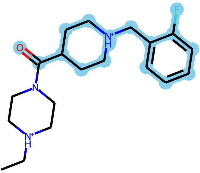 -3.61
-3.61
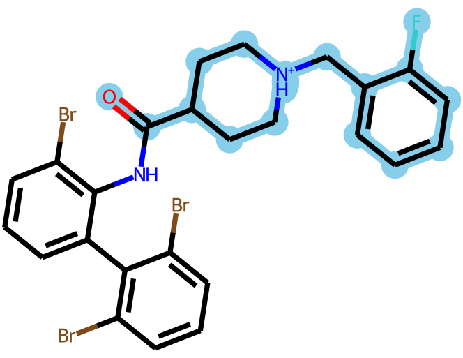 2.36
2.36
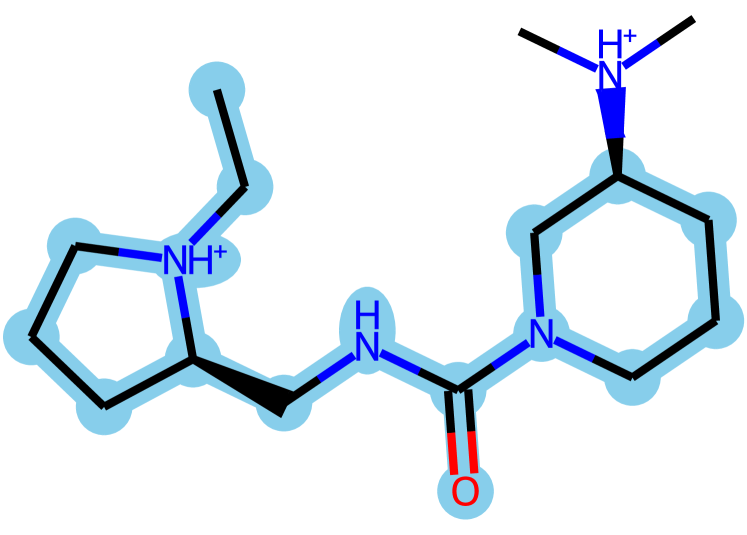 -5.79
-5.79
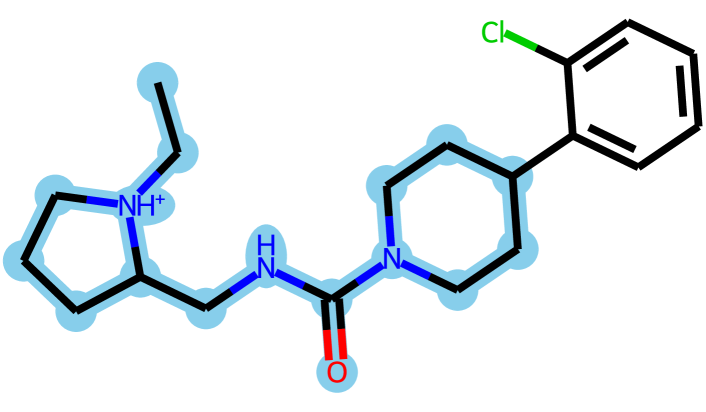 -1.11
-1.11
-1.52
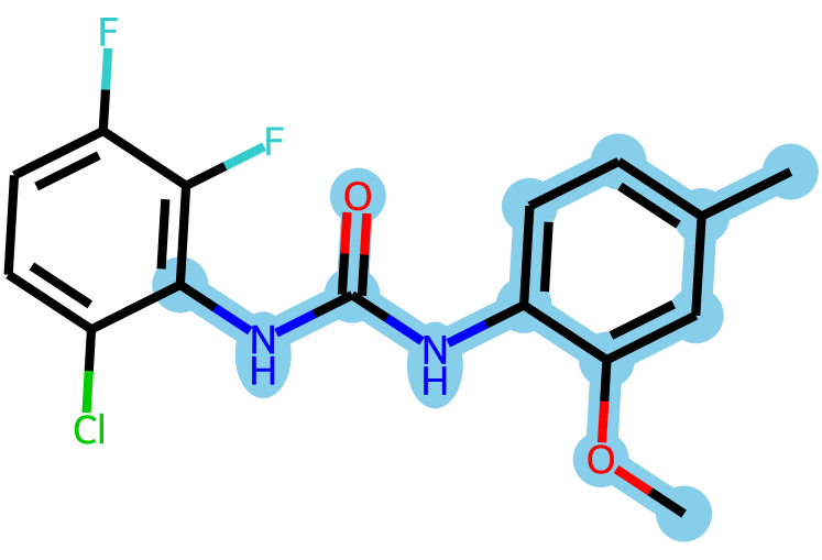 2.90
2.90
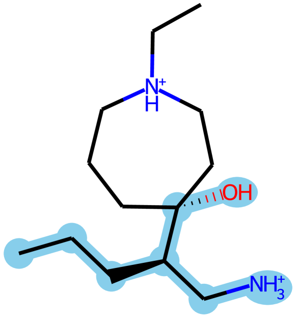 -8.88
-8.88
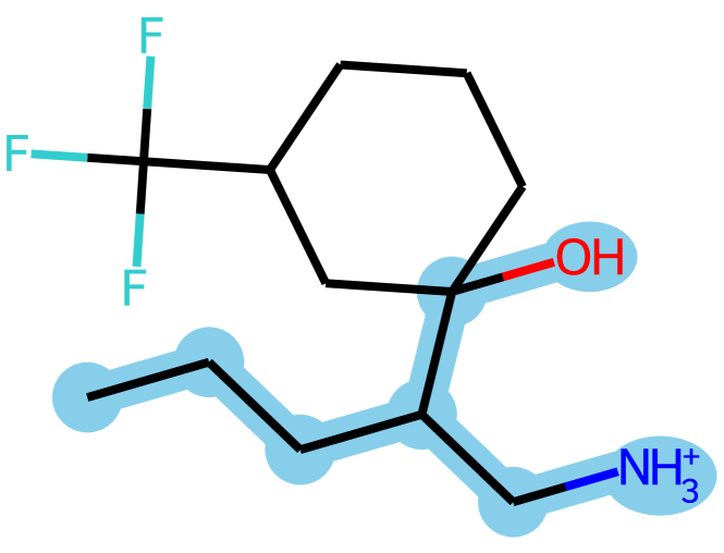 -1.87
-1.87
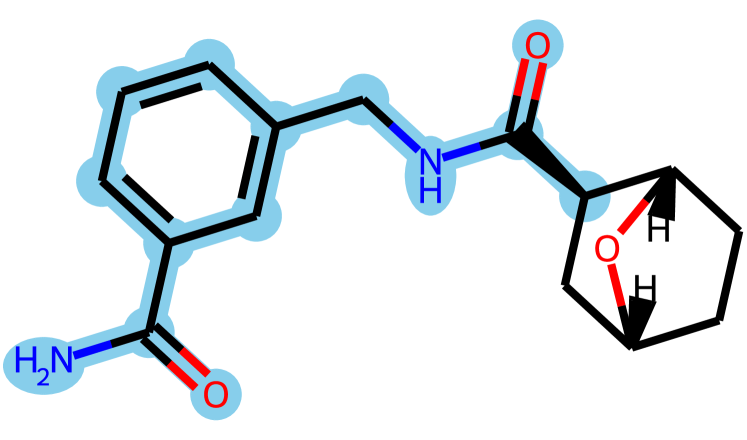 -4.37
-4.37
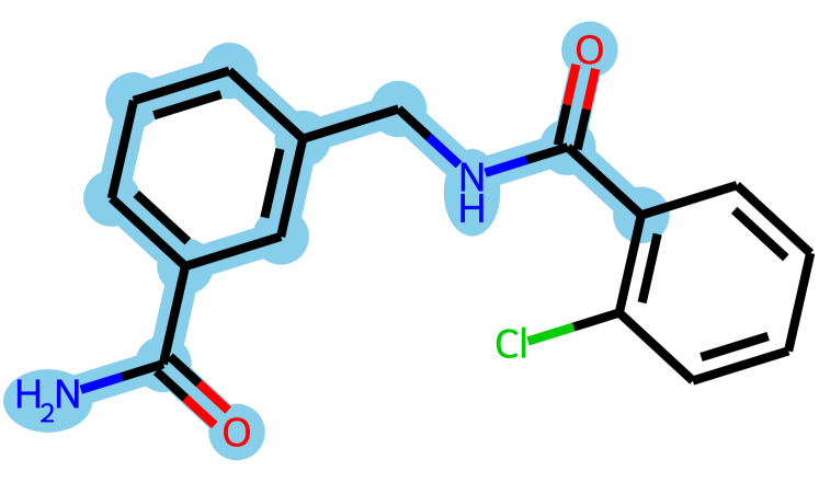 3.26
3.26
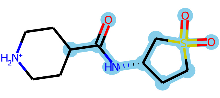 -4.07
-4.07
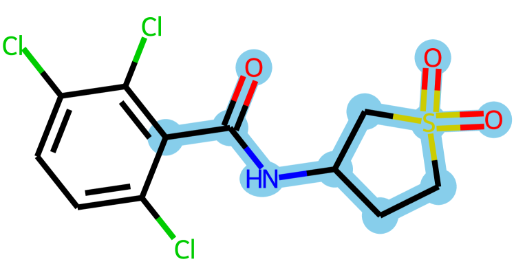 0.60
0.60
Fig. 4(a) shows that Modof-pipe is able to significantly improve pP (mean value changed from -2.75 to 2.25 due to the Modof-pipe optimization). Among the improved pP values, improvement from P contributes most as Fig. 4(b) shows, where P mean values changed from -1.40 to 2.85. Even though, SA scores are also improved by Modof-pipe as in Fig. 4(c), where the mean value of SA scores is improved from -1.30 to -0.64. This indicates that while focusing on learning how to improve P via fragment-based modification, Modof-pipe is also able to learn and incorporate synthetic accessibility into its modification process, and generate new molecules that are even better synthesizable. Fig. 4(d) shows the improvement of SA scores and circle scores together. Note that circle scores are small if there are large rings, which are not preferable for synthesis. The improvement of SA and circle scores together also indicates that Modof-pipe modifies molecules into more synthesizable ones.
Chemical Transformation via Modof-pipe Optimization
Retained scaffolds after optimization are highlighted in sky blue.
Same atoms with different formal charges after optimization are highlighted in orange.
Numbers associated different methods are the corresponding pP values.
(a) 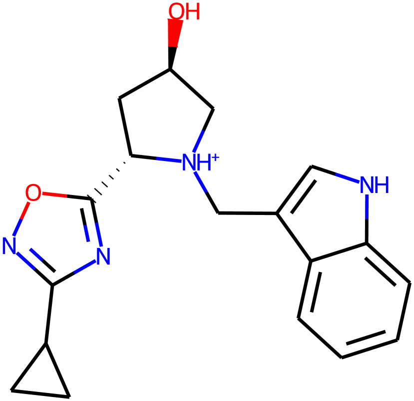 -2.36
-2.36
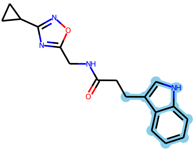 JTNN 1.26
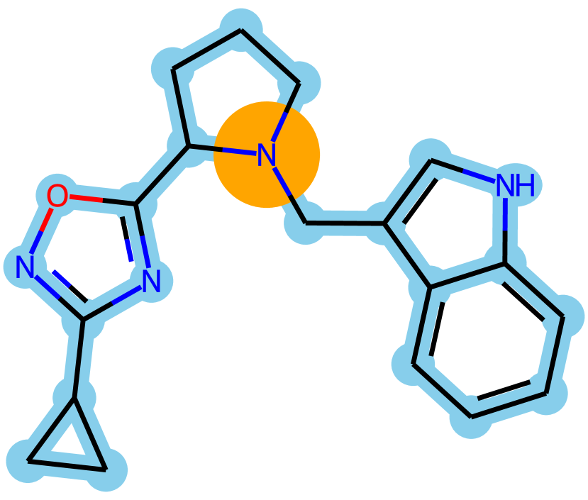 HierG2G 1.32
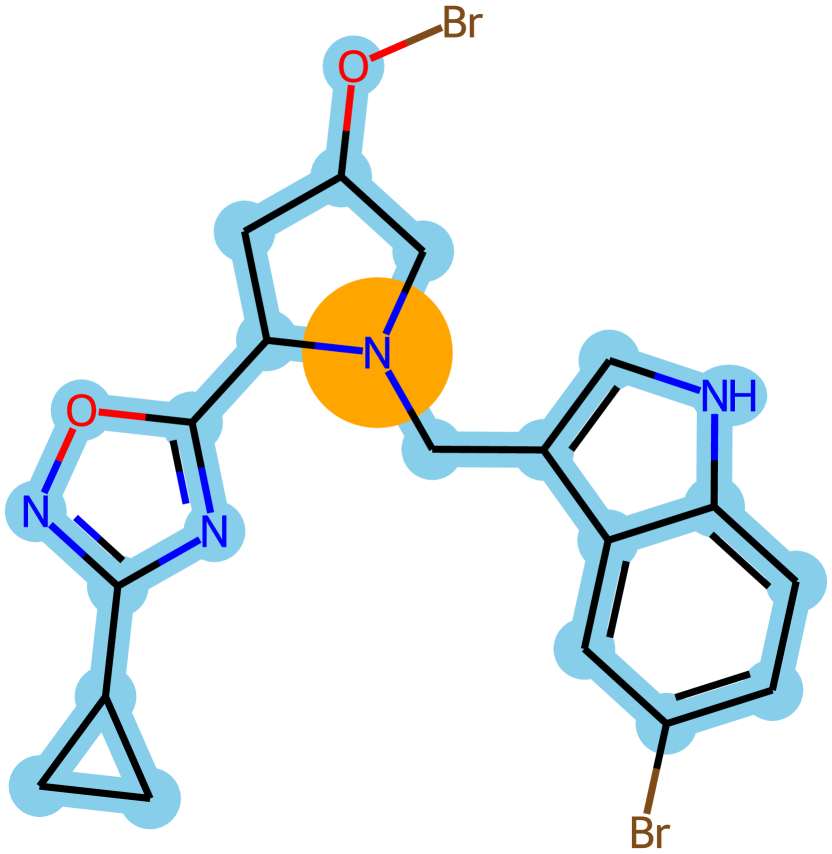 GraphAF 0.97
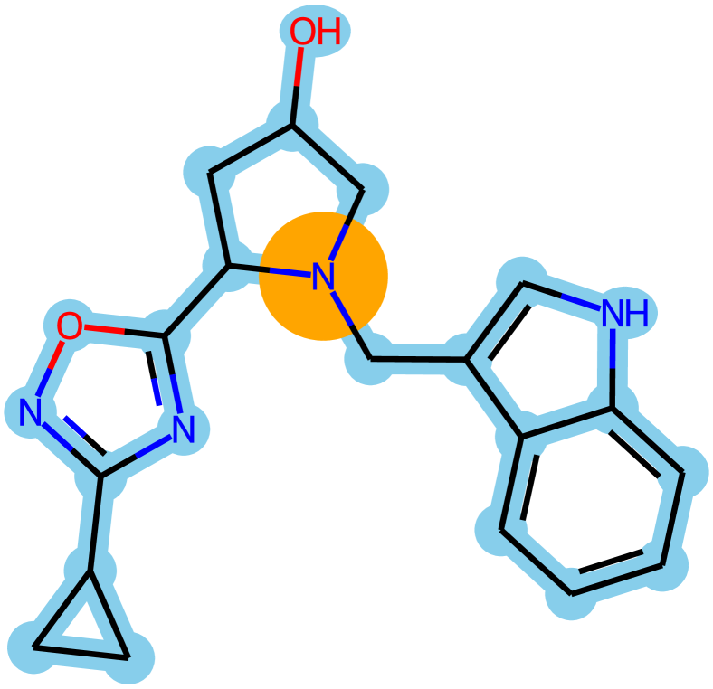 MoFlow 0.07
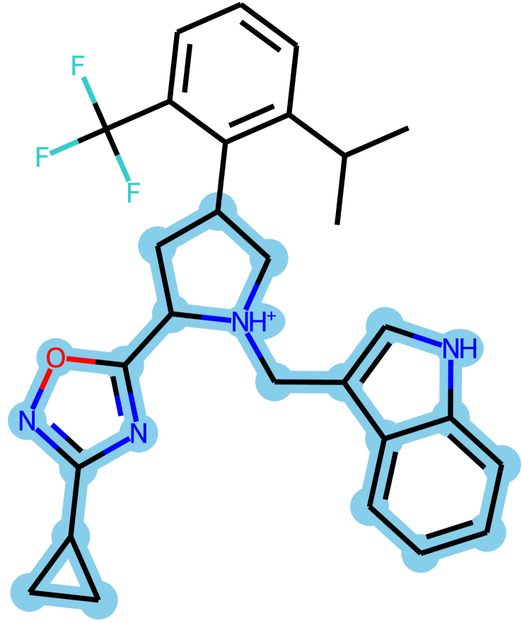 Modof-pipe 0.82
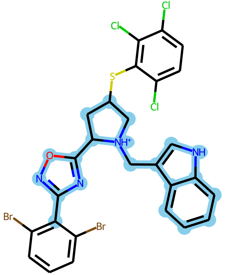 Modof-pipem 2.40
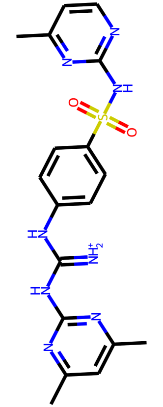 -0.85
-0.85
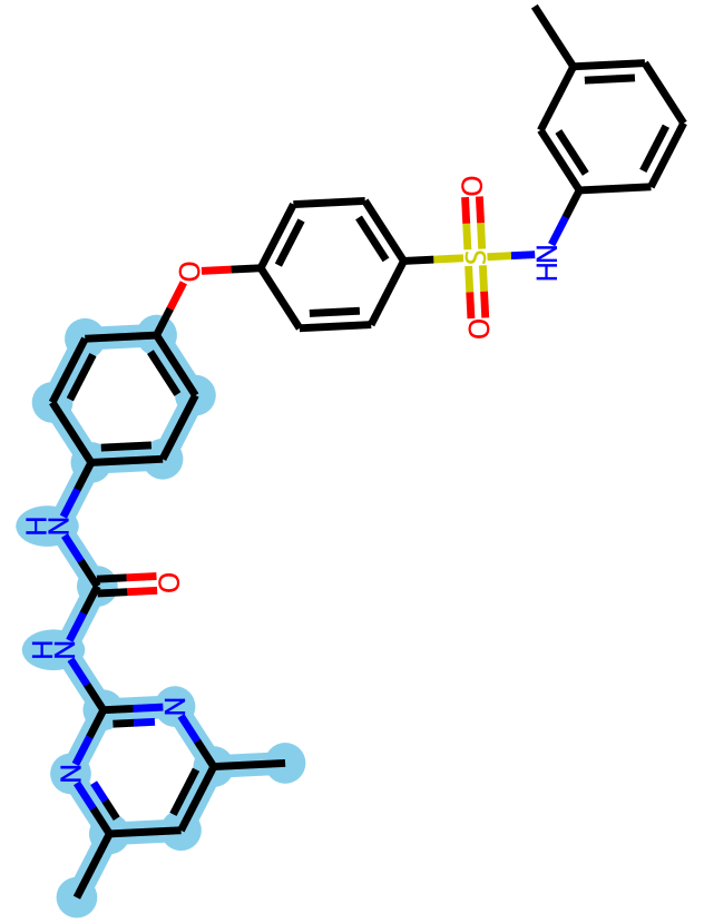 JTNN 3.37
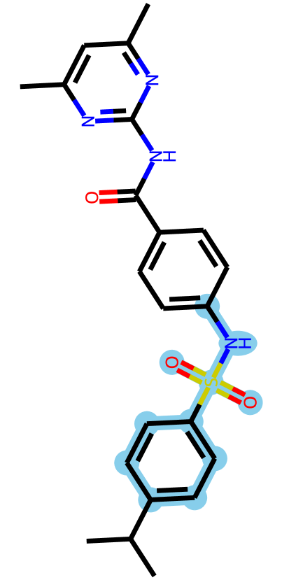 HierG2G 2.61
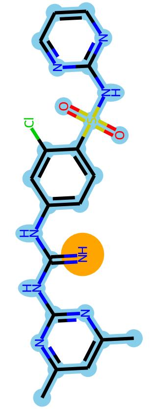 GraphAF 0.77
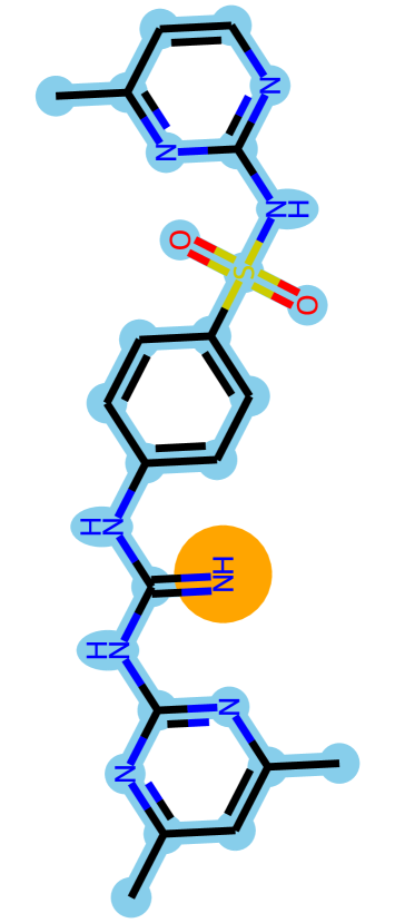 MoFlow 0.63
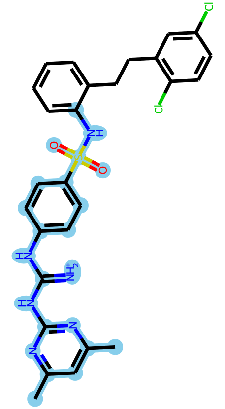 Modof-pipe 1.93
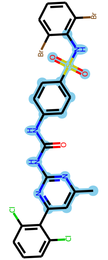 Modof-pipem 4.37
An important aspect of chemical optimization is to search for and explore a novel chemical subspace where molecules have better properties [59]. To analyze whether the optimized molecules given by Modof-pipe reside in a novel chemical subspace compared to the subspace of those before optimization, we conducted the following analysis. We clustered the following five groups of molecules all together: (1) the molecules in training pairs that have bad properties, denoted as ; (2) the molecules in training pairs that have good properties, denoted as ; (3) the molecules in the benchmark test dataset, denoted as (); (4) the optimized test molecules by Modof-pipe with similarity constraint =0.4, denoted as ; and (5) the rest, all the ZINC dataset molecules that are not in the above four groups. We did the clustering in a same way as in Section S3.1 using CLUTO. The clustering results represent how the ZINC chemical space looks, and how molecules are distributed in the ZINC chemical space.
Fig. S5 presents the results from 56 clusters that are sorted in the same way as in Section S3.1. Fig. 5(a) and Fig. 5(b) show that the test molecules and their optimized ones have roughly similar distributions over ZINC clusters (e.g., more distributed in cluster 40 - 50). This indicates that Modof-pipe optimization is not biased at a certain chemical subspace. On the other hand, the distributions still have some notable difference, for example, before optimization, about 8% of test molecules were in cluster 23; after optimization, only 4% of the optimized molecules are in cluster 23. Actually, among the 800 test molecules, 24.38% of the molecules changed to different clusters after Modof-pipe optimization. Compared to test molecules, among the training data, only about 9.20% of have their paired in a different cluster. Fig. S6 shows the examples of test molecules for which their optimized molecules changed to different clusters. The analysis results indicate that Modof-pipe is able to learn from training data (training chemical subspace), and also explore and transform into novel chemical subspaces. Note that Modof-pipe always constrains that the optimized molecules are at least -similar to those before optimization (in this analysis, =0.4). Under this constraint, the fact that Modof-pipe is able to find novel chemical subspaces for about 24% of test molecules indicates its strong exploration capability over the entire chemical space for molecule optimization.
Comparison on Retaining Molecule Scaffolds
Fig. S7 presents two examples of molecules optimized by the four baseline methods, Modof-pipe and Modof-pipem, with similarity constraint =0.4. In these two examples, JTNN tends to insert a new structure within the middle of the molecules. HierG2G could have either very minor (in Fig. 7(a)) or very dramatic (Fig. 7(b)) change to the major molecular scaffolds. Both GraphAF and MoFlow tend to have very small modifications and therefore pP improvement from these two methods is also small. Modof-pipe and Modof-pipem tend to change the periphery of the molecules but can guarantee to retain the major scaffolds of the molecules, with substantial pP improvement.
Model Complexity Comparison
| model | number of parameters |
|---|---|
| JT-VAE | 4.53M |
| GCPN | 6.00M |
| JTNN (=0.4) | 3.74M |
| JTNN (=0.6) | 3.15M |
| HierG2G | 6.80M |
| GraphAF | 1.86M |
| MoFlow | 130.35M |
| Modof (=0.0) | 0.56M |
| Modof (=0.2) | 0.54M |
| Modof (=0.4) | 1.89M |
| Modof (=0.6) | 0.51M |
Table S4 presents the number of parameters of baselines and our models. As shown in this table, the optimal Modof has 0.56M parameters with , 0.54M parameters with , 1.89M parameters with and 0.51M parameters with , which are far less than those in the best baselines. For example, JTNN has 3.74M parameters with and 3.15M with , and HierG2G has 6.8M parameters, that is, Modof uses at least 40% fewer parameters and 26% less training data but outperforms or achieves very comparable results as these state-of-the-art baselines.
Parameters for Reproducibility of pP Optimization
| Hyper-parameters | Space |
|---|---|
| hidden layer dimension | {32, 64, 128, 256} |
| atom/node embedding dimension | {32, 64, 128, 256} |
| / dimension | {8, 16, 32} |
| # iterations of | {3, 4, 5, 6} |
| # iterations of | {2, 3, 4} |
| # sampling | 20 |
We implemented our models using Python-3.6.9, Pytorch-1.3.1, RDKit-2019.03.4 and NetworkX-2.3. We trained the models using a Tesla P100 GPU and a CPU with 16GB memory on Red Hat Enterprise 7.7. We tuned the hyper-parameters of our models with the grid-search algorithm in the parameter space presented in Table S5. We determined the optimal hyper-parameters according to their corresponding pP property improvement over the validation molecules. To optimize a molecule, we randomly sampled =20 latent vectors in each Modof iteration.
For =, the optimal dimension of all the hidden layers is 128, and the dimension of latent embedding is 16 (i.e., 8 for and , respectively), in Modof. The optimal iterations of graph message passing and tree message passing are 6 and 4, respectively. For =, the optimal dimension of all the hidden layers is 128, and the dimension of latent embedding is 32, and the optimal iterations of and are 5 and 4, respectively. For =, the optimal dimension of all the hidden layers is 256, and the dimension of latent embedding is 32, and the optimal iterations of and are 6 and 3, respectively. For =, the optimal dimension of all the hidden layers is 128, the dimension of latent embedding is 32, and the optimal iterations of and are 4 and 3, respectively.
We optimized the models with learning rate 0.001 and batch size 32. During the training period, we did not use regularization and dropout and used default random number seeds in Pytorch to sample the noise variables employed in the reparameterization trick of VAE. The best performance was typically achieved within 7 epochs of training. We set the KL regularization weight in the loss function (Equation 11 in the main manuscript) as 0.1 in the first epoch, and increased its value by 0.05 every 500 batches until 0.5.
Fragment and Molecule Size Analysis in Training Data for pP Optimization
Among the training molecules for pP optimization, the top-5 most popular fragments that have been removed from are: O[C:1] (6.43%), N#[C:1] (4.56%), [O-][C:1] (3.23%), [NH3+][C:1] (2.44%), N[C:1]=O (2.17%); the top-5 most popular fragments to be attached into are: CCSc1cccc[c:1]1 (13.92%), Clc1ccc([C:1])cc1 (12.12%), Clc1c[c:1]ccc1 (6.24%), Clc1cccc[c:1]1 (4.67%), c1ccc2sc([C:1])nc2c1 (4.00%). These removal and attaching fragments are visualized in Fig. 1a and Fig. 1b in the main manuscript.
Overall, the removal fragments in training data are on average of 2.85 atoms and the new attached fragments are of 7.55 atoms. In addition, 39.48% molecules do not have fragments removed and only have new attached fragments, while only 1.78% molecules do not have new fragments attached and only have fragments removed. This shows that in training data, the optimization of pP is typically done via removing small fragments and then attaching larger fragments. This is also reflected in Table S3 (“#”, “#”) that out of each Modof iteration, the optimized molecules become larger. We observed the similar trend from JT-VAE and JTNN that their optimized molecules are also larger than those before optimization. In the benchmark data, larger molecules typically have better pP values (e.g., the correlation between molecule size and pP values is 0.42).
Experimental Results on DRD2 and QED Optimization
In addition to improving pP, another two popular benchmarking tasks for molecule optimization include improving molecule binding affinities against the dopamine D2 receptor (DRD2), and improving the drug-likeness estimated by quantitative measures (QED) [33]. Specifically, given a molecule that doesn’t bind well to the DRD2 receptor (e.g., with low binding affinities), the objective of optimizing DRD2 property is to modify the molecule into another one that will better bind to DRD2. How well the molecules bind to DRD2 is assessed by a support vector machine classifier developed by Olivecrona et al. [34], which predicts a DRD2 score to measure the binding. In the QED task, given a molecule that is not much drug-like, the objective of optimizing QED property is to modify this molecule into a more “drug-like” molecule. The drug-likeness of molecules is quantified by comparing them with approved drugs on eight widely used molecular properties such as the number of aromatic rings and molecular polar surface area [33]. Note that for these two tasks, Modof does not restrict the size of the optimized molecules.
Training Data Generation for DRD2 and QED Optimization
| description | DRD2 | QED |
| #training molecules | 59,696 | 83,161 |
| #training (, ) pairs | 125,469 | 92,045 |
| #validation molecules | 500 | 360 |
| #test molecules | 1,000 | 800 |
| average similarity of training (, ) pairs | 0.6803 | 0.6578 |
| average pairwise similarity between training and test molecules | 0.1366 | 0.1227 |
| average training molecule size | 28.76 | 23.22 |
| average training size | 28.81 | 24.38 |
| average training size | 28.66 | 22.06 |
| average test molecule size | 24.57 | 22.81 |
| average score | 0.1827 | 0.7500 |
| average score | 0.5366 | 0.8768 |
| average testing molecule score | 0.0067 | 0.7528 |
| average score improvement in training (, ) pairs | 0.4013 | 0.1355 |
We used the CheMBL dataset [60] processed by Olivecrona et al. [34]. This processed CheMBL dataset has 1,179,477 molecules in total, and each molecule is restricted to have 10 to 50 heavy atoms and only contains atoms in {H, B, C, N, O, F, Si, P, S, Cl, Br, I}. We constructed our training data from this processed CheMBL dataset as follows. We first identified 7,743,098 pairs of molecules with similarities from this CheMBL dataset. We selected this high similarity threshold because Modof requires training pairs different in only one fragment at one disconnection site, and thus should be very similar. Among these similar molecule pairs, we selected the pairs that satisfy the following property constraints, respectively: for the DRD2 optimization task, the DRD2 score difference of the two molecules in a pair should be at least 0.2, that is,
| (S1) |
for the QED optimization task, the QED score difference of the two molecules in a pair should be at least 0.1, that is,
| (S2) |
Among the molecule pairs that satisfied the above property constraints, respectively, we identified the pairs in which the two molecules are different only at one disconnection site. Through all these processes, we finally identified 125,469 training pairs for the DRD2 task and 92,045 training pairs for the QED task. The test set for the DRD2 and QED tasks is the benchmark datasets provided by Jin et al. [14] and contains 1,000 molecules and 800 molecules, respectively. Table S6 presents the data statistics for the DRD2 and QED tasks.
Disconnection sites are highlighted in yellow.


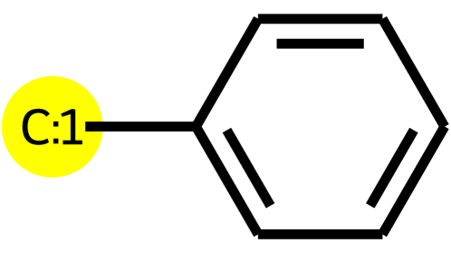
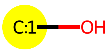
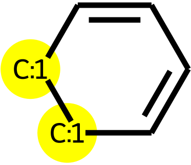
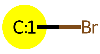

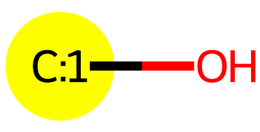
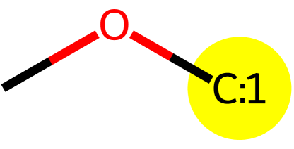

Fragment and Molecule Size Analysis for DRD2 and QED Optimization
Among the training molecules for the DRD2 optimization task, the top-5 most popular fragments that have been removed from are: CO[C3:1] (2.90%), C[C3:1] (2.29%), C1C[N:1]CCO1 (1.67%), c1cc[cH:1]cc1 (1.63%), O=[N+]([O-])[C:1] (1.61%); the top-5 most popular fragments to be attached into are: Cl[C:1] (4.21%) F[C:1] (4.13%) C[C:1] (1.95%) c1cc[c:1]cc1 (1.89%) O[C:1] (1.59%). Overall, the attaching fragments are on average of 6.46 atoms and the removed fragments are of 6.51 atoms. In addition, 7.08% molecules do not have new fragments attached and only have fragments removed, while 9.20% do not have fragments removed and only have fragments attached. Unlike in pP training data, molecules in DRD2 training data do not have significant difference in size when they have different DRD2 properties. Fig. S8 presents the popular removal and attaching fragments among DRD2 training molecules.
Among the training molecules for the QED optimization task, the top-5 most popular fragments that have been removed from are: c1cc[c:1]cc1 (4.04%), c1ccc([C:1])cc1 (2.52%), O[C:1] (2.20%), C1=C[C:1][C:1]C=C1 (2.03%), Br[C:1] (1.44%); the top-5 most popular fragments to be attached into are: C[C:1] (5.10%), O[C:1] (3.40%), CO[C:1] (2.69%), C[C:1]C (2.57%), c1cc[c:1]cc1 (2.55%). Overall, the attaching fragments are on average of 4.17 atoms and the removed fragments are of 6.78 atoms. In addition, 17.62% molecules do not have new fragments attached and only have fragments removed, while only 5.02% molecules do not have fragments removed and only have fragments attached. Unlike in pP and DRD2 training data, molecules in QED training data tend to be smaller when they have better QED properties. Fig. S9 presents the popular removal and attaching fragments among QED training molecules.
Baseline Methods
We used JTNN [14] and HierG2G [15] as the baseline methods to compare Modof with. These two methods have been demonstrated to achieve the state-of-the-art performance on DRD2 and QED optimization [15]. Note that in the original JTNN and HierG2G manuscripts, their training data are different from the training data we generated as in Section S11.1: in their training data, molecule pairs have a similarity difference not below 0.4 (); for the DRD2 task, the DRD2 score of molecule is in and in ; for the QED task, the QED score of molecule is in and to be . To allow a fair comparison, we also trained JTNN and HierG2G on Modof’s training data, and the corresponding models are denoted as JTNN(m) and HierG2G(m), respectively.
Same as in the pP task, in each iteration, Modof samples 20 times from its latent space and decodes 20 output molecules. In Modof-pipe, the best molecule which satisfies the corresponding similarity constraint and has positive improvement on DRD2 or QED at each iteration will be fed into the next iteration for further optimization. Each test molecule will be optimized with at most five iterations. In addition to Modof-pipe, Modof-pipem is also applied to enable multiple optimized molecules as output.
| model | () | (imprv 0.2) | ||||||||||
| rate% | imprvstd | simstd | rate% | imprvstd | simstd | rate% | imprvstd | simstd | ||||
| 0.4 | JTNN | 78.90 | 0.830.18 | 0.440.05 | 78.10 | 0.830.17 | 0.440.05 | 78.30 | 0.830.17 | 0.440.05 | ||
| HierG2G | 85.40 | 0.810.20 | 0.440.05 | 82.00 | 0.830.16 | 0.440.05 | 84.00 | 0.820.18 | 0.440.05 | |||
| JTNN(m) | 84.40 | 0.490.32 | 0.490.08 | 43.50 | 0.770.15 | 0.490.08 | 61.60 | 0.650.24 | 0.490.08 | |||
| HierG2G(m) | 91.50 | 0.530.32 | 0.490.08 | 51.80 | 0.780.15 | 0.490.08 | 70.20 | 0.660.24 | 0.490.08 | |||
| Modof-pipe | 98.80 | 0.690.29 | 0.480.07 | 74.90 | 0.830.14 | 0.480.07 | 89.00 | 0.750.22 | 0.480.07 | |||
| Modof-pipem | 99.10 | 0.820.22 | 0.460.05 | 88.60 | 0.880.12 | 0.460.05 | 95.90 | 0.840.18 | 0.460.05 | |||
| 0.5 | JTNN | 13.40 | 0.730.23 | 0.540.05 | 12.50 | 0.780.17 | 0.540.05 | 12.60 | 0.770.17 | 0.540.04 | ||
| HierG2G | 22.40 | 0.630.32 | 0.550.05 | 16.20 | 0.800.16 | 0.540.05 | 18.50 | 0.750.21 | 0.540.05 | |||
| JTNN(m) | 64.90 | 0.350.32 | 0.570.07 | 22.50 | 0.740.15 | 0.570.07 | 35.80 | 0.590.23 | 0.570.06 | |||
| HierG2G(m) | 78.10 | 0.390.33 | 0.570.07 | 30.80 | 0.750.15 | 0.560.06 | 45.80 | 0.610.24 | 0.570.06 | |||
| Modof-pipe | 94.20 | 0.490.34 | 0.560.05 | 47.70 | 0.790.15 | 0.560.05 | 66.80 | 0.660.24 | 0.560.05 | |||
| Modof-pipem | 97.80 | 0.630.32 | 0.540.04 | 66.60 | 0.820.14 | 0.540.04 | 83.20 | 0.720.23 | 0.540.04 | |||
| 0.6 | JTNN | 1.60 | 0.690.25 | 0.650.03 | 1.40 | 0.760.16 | 0.640.03 | 1.40 | 0.760.16 | 0.640.03 | ||
| HierG2G | 4.40 | 0.500.35 | 0.650.04 | 2.60 | 0.770.15 | 0.640.04 | 3.10 | 0.700.21 | 0.650.04 | |||
| JTNN(m) | 41.40 | 0.230.28 | 0.670.06 | 8.40 | 0.720.15 | 0.660.06 | 15.50 | 0.540.23 | 0.660.05 | |||
| HierG2G(m) | 52.00 | 0.240.28 | 0.660.06 | 10.50 | 0.720.14 | 0.660.05 | 19.70 | 0.540.23 | 0.660.05 | |||
| Modof-pipe | 79.60 | 0.270.31 | 0.650.04 | 19.70 | 0.750.15 | 0.640.03 | 32.40 | 0.590.24 | 0.640.03 | |||
| Modof-pipe-5 | 87.50 | 0.340.33 | 0.640.04 | 28.90 | 0.760.15 | 0.640.03 | 45.30 | 0.610.24 | 0.630.03 | |||
-
•
Columns represent: “rate%”: the percentage of optimized molecules in each group (, , ) over all test molecules; “imprv”: the average property improvement; “std”: the standard deviation; “sim”: the similarity between the original molecules and optimized molecules . Best rate% values are in bold.
Evaluation Metrics
We compared different methods by analyzing the following three groups of molecules:
-
•
Optimized molecules (): If an input molecule is optimized into with any better properties, that is, no constraints on how much better is than , and also satisfies the similarity constraint with (i.e., ), this molecule is considered as optimized.
-
•
under property improvement constraints (): We also measured the optimized molecules ( defined as above) that achieved a certain property improvement, following JTNN and HierG2G’s criteria:
-
(1)
For DRD2, the optimized molecules should have DRD2 score no less than 0.5, that is,
(S3) -
(2)
For QED, the optimized molecules should have QED score no less than 0.9, that is,
(S4)
-
(1)
-
•
following training data property constraints (): a potential issue with is that if in the training molecule pairs, the property improvement constraints are not satisfied, imposing the constraints in for evaluation is overkilling and tends to underestimate the model performance. Therefore, we also measured the optimized molecules ( defined as above) that achieved property improvement in a similar degree as in training data:
Among each of these three groups of molecules, we measured 1) the percentage of the optimized molecules from that group over all test molecules, referred to as success rate, denoted as rate%, 2) within each group, the average property improvement of optimized over , and 3) within each group, the average similarity values between and . Note that rate% in is identical to the success rate used in Jin et al. [14](JTNN) and Jin et al. [15](HierG2G).
Experimental Results
Experimental Results on Optimizing DRD2
Table S7 presents the overall comparison between the baseline methods JTNN, HierG2G, JTNN(m), HierG2G(m) and our methods Modof-pipe and Modof-pipem on optimizing the DRD2 property. Please note that JTNN and HierG2G used a training dataset generated based on their criteria [14]; JTNN(m), HierG2G(m), Modof-pipe and Modof-pipem used the training data generated as described in Section S11.1; all the methods were tested on the same benchmark test set provided by Jin et al. [14] that contains 1,000 molecules. We stratified JTNN, JTNN(m), HierG2G and HierG2G(m)’s optimized molecules ’s using their similarities with respect to corresponding ’s. We used the similarity thresholds =0.4, 0.5 and 0.6 for the stratification, which also define the similarity constraints in Modof-pipe and Modof-pipem. For Modof-pipem, the property improvement and optimized molecule similarities to those before optimization are always considered on the best optimized molecule among all the optimized molecules. Under each similarity constraint , the optimized molecules within each of the , and groups are always at least -similar to the molecules before optimization.
Table S7 shows that Modof-pipem consistently achieves the highest success rates of optimized molecules, when considering molecules that are ever optimized (in ), or optimized with a certain property improvement (in and ), under all the similarity constraints (=0.4, 0.5 and 0.6). With similarity constraint =0.4, that is, each optimized molecule has a similarity at least 0.4 with its corresponding before optimization, Modof-pipem is able to improve the DRD2 property for 99.10% of all the test molecules in ; this is a 8.31% improvement over the best baseline method HierG2G(m), which achieves a 91.5% success rate. Among the optimized molecules in , the average DRD2 property improvement (“imprvstd”) from Modof-pipem (0.820.22) is among the best compared to the results from other baseline methods (e.g., 0.830.18 from JTNN); the average pair-wise similarities between the test molecules and their optimized molecules from Modof-pipem (0.460.05) are also comparable to those of other methods. Compared to with =0.4, the optimized molecules in and have a lower success rate because not all the optimized molecules in have or DRD2 improvement no less than 0.2. However, Modof-pipem still achieves the best success rates (88.60% in and 95.90% in , respectively) compared to the baseline methods. In terms of the property improvement among the optimized molecules in , Modof-pipem achieves the best (0.880.12); in terms of pair-wise similarities, Modof-pipem has very comparable performance (0.460.05) compared to the baseline methods. The same conclusions hold true in .
With similarity constraint =0.5 and 0.6, we observed the same trends as those with =0.4: consistently in , and , Modof-pipem achieves the best success rates (rate%), best or competitive property improvement (imprvstd), and competitive pair-wise similarities (simstd) between the test molecules and their optimized molecules. Particularly, with =0.5 and 0.6, Modof-pipem’s success rates in , and were substantially higher than those of the baseline methods: for example, with =0.5 and 0.6 in , Modof-pipem has a 116.23% and 175.24%, respectively, higher rate% than that of HierG2G(m) (66.60% vs 30.80%; 28.90% vs 10.50%); in , Modof-pipem’s rate% is 81.66% and 129.95%, respectively, higher than that of HierG2G(m) (83.20% vs 45.80%; 45.30% vs 19.70%). This demonstrates the strong capability of Modof-pipem in optimizing molecules and improving DRD2 properties.
| model | (0.9) | (imprv0.1) | ||||||||||
| rate% | imprvstd | simstd | rate% | imprvstd | simstd | rate% | imprvstd | simstd | ||||
| 0.4 | JTNN | 71.00 | 0.160.04 | 0.470.06 | 60.50 | 0.170.03 | 0.470.06 | 67.38 | 0.170.03 | 0.470.07 | ||
| HierG2G | 86.50 | 0.170.04 | 0.460.06 | 75.12 | 0.180.03 | 0.460.06 | 82.38 | 0.170.03 | 0.460.06 | |||
| JTNN(m) | 93.50 | 0.130.06 | 0.550.10 | 40.50 | 0.170.03 | 0.540.09 | 68.50 | 0.150.03 | 0.540.09 | |||
| HierG2G(m) | 91.75 | 0.130.06 | 0.520.10 | 37.12 | 0.170.03 | 0.520.09 | 65.88 | 0.150.03 | 0.530.10 | |||
| Modof-pipe | 96.38 | 0.130.05 | 0.520.09 | 40.00 | 0.170.03 | 0.510.08 | 70.00 | 0.160.03 | 0.510.08 | |||
| Modof-pipe-5 | 99.12 | 0.150.04 | 0.480.07 | 66.25 | 0.180.03 | 0.480.07 | 87.62 | 0.170.03 | 0.480.07 | |||
| 0.5 | JTNN | 42.38 | 0.150.04 | 0.560.05 | 30.25 | 0.170.03 | 0.550.05 | 37.88 | 0.160.03 | 0.560.05 | ||
| HierG2G | 55.00 | 0.160.04 | 0.550.05 | 40.38 | 0.170.03 | 0.550.05 | 50.38 | 0.160.03 | 0.550.05 | |||
| JTNN(m) | 86.62 | 0.120.06 | 0.600.08 | 30.50 | 0.170.03 | 0.600.07 | 56.12 | 0.150.03 | 0.600.07 | |||
| HierG2G(m) | 84.25 | 0.110.06 | 0.590.08 | 26.75 | 0.170.03 | 0.590.06 | 53.25 | 0.150.03 | 0.600.07 | |||
| Modof-pipe | 89.25 | 0.120.05 | 0.590.07 | 27.25 | 0.170.03 | 0.580.06 | 53.62 | 0.150.03 | 0.580.06 | |||
| Modof-pipe-5 | 98.62 | 0.130.05 | 0.560.06 | 43.38 | 0.170.03 | 0.560.05 | 71.25 | 0.160.03 | 0.560.05 | |||
| 0.6 | JTNN | 17.62 | 0.130.05 | 0.650.05 | 10.12 | 0.160.03 | 0.650.04 | 13.38 | 0.150.03 | 0.650.04 | ||
| HierG2G | 20.25 | 0.140.06 | 0.650.05 | 12.00 | 0.170.03 | 0.650.04 | 15.75 | 0.160.03 | 0.650.04 | |||
| JTNN(m) | 73.62 | 0.100.07 | 0.680.07 | 18.88 | 0.170.03 | 0.660.06 | 38.62 | 0.150.03 | 0.660.05 | |||
| HierG2G(m) | 70.88 | 0.100.07 | 0.670.06 | 17.38 | 0.170.03 | 0.660.05 | 37.25 | 0.150.03 | 0.660.05 | |||
| Modof-pipe | 66.25 | 0.090.06 | 0.660.05 | 12.25 | 0.160.03 | 0.650.04 | 29.62 | 0.140.03 | 0.650.04 | |||
| Modof-pipe-5 | 89.25 | 0.090.07 | 0.660.05 | 18.62 | 0.170.03 | 0.650.04 | 39.50 | 0.150.03 | 0.650.04 | |||
-
•
Columns represent: “rate%”: the percentage of optimized molecules in each group (, , ) over all test molecules; “imprv”: the average property improvement; “std”: the standard deviation; “sim”: the similarity between the original molecules and optimized molecules . Best rate% values are in bold.
Experimental Results on Optimizing QED
Table S8 presents the overall comparison between the baseline methods JTNN, HierG2G, JTNN(m), HierG2G(m) and our methods Modof-pipe and Modof-pipem on optimizing the QED property. Overall, the trends are very similar with what we observed in DRD2 optimization: Modof-pipem achieves the best success rates in , and with all the similarity constraints (=0.4, 0.5 and 0.6), except in with =0.4 and 0.6, where Modof-pipem has the second best success rates (with =0.6, the difference with the best success rate is very minimum).
Parameters for Reproducibility of Optimizing DRD2 and QED
We tuned the hyper-parameters of our models for DRD2 and QED optimization tasks with the grid-search algorithms in the parameter spaces as presented in Table S9. We determined the optimal hyper-parameters according to the success rate rate% of Modof-pipe in under =0.4 over the validation molecules provided by Jin et al. [14]. In each iteration, we randomly sampled =20 latent vectors and output 20 optimized candidates.
For DRD2, the optimal dimension of all the hidden layers is 320 and the dimension of latent embedding is 64 (i.e., 32 for and , respectively). The optimal iterations of graph message passing and tree message passing are 6 and 5, respectively. The optimal Modof for DRD2 has 3.09M parameters and can achieve the best performance with 3 epochs of training. For QED, the optimal dimension of all the hidden layers is 256 and the dimension of latent embedding is 32 (i.e., 16 for and , respectively). The optimal iterations of graph message passing and tree message passing is 4. The optimal Modof for QED has 1.81M parameters and can achieve the best performance with 4 epochs of training. Other training details such as learning rate and KL regularization weight are the same as demonstrated in Section S9.8.
| Hyper-parameters | Space |
|---|---|
| hidden layer dimension | {64, 128, 256, 320} |
| atom/node embedding dimension | {64, 128, 256, 320} |
| / dimension | {8, 16, 32} |
| # iterations of | {4, 5, 6, 7} |
| # iterations of | {3, 4, 5} |
| # sampling | 20 |
Experimental Results on Multi-Property Optimization of DRD2 and QED
Here we demonstrate the effectiveness of Modof for multi-property optimization. We conduct experiments to simultaneously improve two molecular properties (QED and DRD2). Specifically, given a molecule that is not much drug-like (i.e., with a low DRD2 score) and doesn’t bind well to the DRD2 receptor (i.e., with a low QED score), the objective of the task is to modify this molecule to a drug-like molecule bound well to the DRD2 (i.e., with both high DRD2 and QED scores). The assessment of DRD2 and QED properties is as described in the Section S11.
Training Data Generation for Multi-Property Optimization
We used the training molecule pairs for DRD2 task derived from CheMBL dataset as in Section S11.1 to construct the training data for this multi-property optimization task. Recall that each molecule pair for the DRD2 task has similarity and satisfies the following property constraint:
| (S7) |
Among these molecule pairs, we first selected the pairs that also have differences on QED scores, that is,
| (S8) |
Among the molecule pairs that satisfied the above two property constraints, we first identified the pairs in which two molecules are different only at one disconnection site. We finally identified 14,230 training pairs for this task. The test set for this task includes 800 molecules that do not appear in the training pairs and have the property and . Table S10 presents the data statistics for this multi-property optimization task.
| description | DRD2 & QED |
|---|---|
| #training molecules | 10,121 |
| #training (, ) pairs | 14,230 |
| #validation molecules | 200 |
| #test molecules | 800 |
| average similarity of training (, ) pairs | 0.6721 |
| average pairwise similarity between training and test molecules | 0.1257 |
| average training molecule size | 30.08 |
| average training size | 32.42 |
| average training size | 27.16 |
| average test molecule size | 32.05 |
| average score | 0.1788 |
| average score | 0.4957 |
| average score | 0.5033 |
| average score | 0.6963 |
| average DRD2 score of test molecules | 0.1102 |
| average QED score of test molecules | 0.4241 |
| average DRD2 score improvement in training (, ) pairs | 0.4356 |
| average QED score improvement in training (, ) pairs | 0.2240 |
Fragment and Molecule Size Analysis for Multi-Property Optimization
Among the training molecules for the multi-property optimization task, the top-5 most popular fragments that have been removed from are: O=[N+]([O-])[C3:1] (5.17%), c1cc[c:1]cc1 (1.91%), c1ccc([C3:1])cc1 (1.90%), c1ccc2c(c1)ccc[c:1]2 (1.25%), CO[C3:1] (1.15%); the top-5 most popular fragments to be attached into are: F[C3:1] (5.14%), Cl[C3:1] (3.32%), C[C3:1] (2.99%), O[C3:1] (2.31%), c1cc[c:1]cc1 (2.14%). In addition, 16.75% do not have new fragments attached and only have fragments removed, while only a few do not have fragments removed and only have fragments attached. This is likely due to the fact that smaller molecules have better QED properties.
Baseline Methods
We used the same baselines JTNN and HierG2G as in the DRD2 and QED tasks in Section S11. These two methods have been demonstrated to achieve the state-of-the-art performance on DRD2 and QED optimization, respectively, and thus are strong baselines on the multi-property optimization task on DRD2 and QED. Note that the original JTNN and HierG2G did not have the experiments on this multi-property optimization task in their manuscripts. Therefore, we can only train JTNN and HierG2G with our dataset, and the corresponding models are denoted as and , respectively.
Same as in the single-property optimization task, in each iteration, Modof sampled 20 times from its latent space and decodes 20 output molecules. At each iteration, Modof-pipe and Modof-pipem used the sum of DRD2 and QED scores to select the best optimized molecules under the corresponding similarity constraint. The selected molecules were fed into the next iteration for further optimization. Each test molecule was optimized in at most five iterations.
| model | () | () | ( && ) | ||||||||||
|---|---|---|---|---|---|---|---|---|---|---|---|---|---|
| rate% | imprvstd | simstd | rate% | imprvstd | simstd | rate% | imprvstd | simstd | |||||
| 0.4 | JTNN(m) | 10.62 | 0.530.20 | 0.540.11 | 21.00 | 0.270.13 | 0.550.12 | 8.62 | 0.820.22 | 0.550.11 | |||
| HierG2G(m) | 15.62 | 0.580.18 | 0.510.10 | 26.00 | 0.300.13 | 0.510.10 | 14.50 | 0.850.21 | 0.510.10 | ||||
| Modof-pipe | 48.88 | 0.630.17 | 0.510.10 | 54.00 | 0.320.13 | 0.490.08 | 24.62 | 0.920.20 | 0.490.08 | ||||
| Modof-pipem | 67.75 | 0.710.15 | 0.470.07 | 82.25 | 0.360.13 | 0.480.07 | 38.88 | 0.950.21 | 0.480.06 | ||||
| 0.5 | JTNN(m) | 6.88 | 0.530.19 | 0.600.09 | 13.12 | 0.260.12 | 0.620.10 | 5.88 | 0.820.21 | 0.600.09 | |||
| HierG2G(m) | 8.38 | 0.550.17 | 0.590.08 | 15.25 | 0.240.12 | 0.600.08 | 7.88 | 0.800.21 | 0.600.08 | ||||
| Modof-pipe | 41.25 | 0.580.17 | 0.590.07 | 44.75 | 0.270.12 | 0.590.07 | 16.62 | 0.820.20 | 0.590.07 | ||||
| Modof-pipem | 58.38 | 0.660.15 | 0.560.06 | 69.25 | 0.320.12 | 0.570.06 | 27.25 | 0.840.23 | 0.570.07 | ||||
| 0.6 | JTNN(m) | 2.88 | 0.490.15 | 0.680.06 | 7.25 | 0.240.11 | 0.700.07 | 2.62 | 0.750.18 | 0.680.06 | |||
| HierG2G(m) | 4.38 | 0.530.15 | 0.660.05 | 8.12 | 0.230.12 | 0.670.06 | 4.12 | 0.750.20 | 0.660.05 | ||||
| Modof-pipe | 26.88 | 0.530.16 | 0.670.06 | 29.12 | 0.240.11 | 0.670.05 | 9.12 | 0.750.19 | 0.670.05 | ||||
| Modof-pipem | 34.12 | 0.580.17 | 0.660.05 | 43.88 | 0.270.11 | 0.660.05 | 13.00 | 0.780.22 | 0.660.06 | ||||
-
•
Columns represent: “ ()”: the optimized molecules that have a DRD2 score no less than 0.5; “ ()”: the optimized molecules that have a QED score no less than 0.6; “ ( && )”: the optimized molecules that have a DRD2 score no less than 0.5 and at the same time a QED score no less than 0.6; “rate%”: the percentage of optimized molecules in each group over all test molecules; “imprv”: the average property improvement on DRD2 or QED for the group () or (), or the average of sum of property improvements on DRD2 and QED scores for the group ( && ); “std”: the standard deviation; “sim”: the similarity between the original molecules and optimized molecules . Best rate% values are in bold.
Evaluation Metrics
Similarly to that in Section S11.3, we compared different methods by analyzing on different groups of molecules as follows in the test set with respect to different property constraints:
-
•
for DRD2: The optimized molecules should have DRD2 score no less than 0.5, that is,
(S9) -
•
for QED: The optimized molecules should have QED score no less than 0.6, that is,
(S10) -
•
for DRD2 and QED: The optimized molecules should have DRD2 score no less than 0.5 and QED score no less than 0.6, that is,
(S11)
Note that in this multi-property optimization task, molecules that have been optimized to have or may or may not satisfy the QED or DRD2 constraint. The group for DRD2 or for QED only includes the optimized molecules that satisfy the DRD2 or QED constraint alone. The group for DRD2 and QED includes the optimized molecules that satisfy both the DRD2 and QED constraints. In other words, this group is the intersection of the above two groups. Among each of these three groups of molecules, we used the success rate rate%, the average property improvement of over , and the average similarity values between and to compare the different results.
Experimental Results
Table S11 presents the overall comparison between the baseline methods and and our methods Modof-pipe and Modof-pipem on the multi-property optimization problem. All the methods were trained for 30 epochs on the same training data as generated in Section S12.1. We then tuned the hyper-parameters and found the best model for each method using a validation set with 200 molecules. The selected best models were tested on the test set that contains 800 molecules. Following Section S11.4, we used the similarity thresholds =0.4, 0.5 and 0.6 to stratify the optimized molecules of all the methods.
Table S11 shows that Modof-pipe and Modof-pipem significantly outperform two baseline methods and on the success rates of optimized molecules under all the similarity constraints (=0.4, 0.5 and 0.6). With similarity constraint =0.4, that is, each optimized molecule has a similarity at least 0.4 with its corresponding before optimization, Modof-pipe and Modof-pipem is able to achieve 24.62% and 38.88% success rates on the group (&&), respectively; these are 69.79% and 168.14% better than the best baseline method (14.50% in (&&)), respectively. With other similarity constraints =0.5 and 0.6, we observed the same trend that Modof-pipe and Modof-pipem consistently outperformed two baseline methods on the results of group (&&). This demonstrates the strong capability of Modof-pipe and Modof-pipem on the multi-property optimization problem.
In addition, Table S11 shows that Modof-pipe and Modof-pipem also outperformed the two baseline methods and with a wide margin on the success rates in group and . With similarity constraint =0.4, Modof-pipe and Modof-pipem were able to achieve 54.00% and 82.25% success rates on the group , respectively; these are 107.69% and 216.34% better the best baseline method (26.00% in (&&)), respectively. This demonstrates that Modof-pipe and Modof-pipem have stronger capabilities to optimize molecules under the similarity constraint towards better properties. Compared to these rate% values on the group in single-property optimization as in Table S11 (54.00% for Modof-pipe and 82.25% for Modof-pipem on QED optimization), the smaller success rates in the multi-property optimization (24.62% for Modof-pipe and 38.88% for Modof-pipem) also indicate that multi-property optimization is a challenging problem.
Parameters for Reproducibility of Multi-Property Optimization
We tuned the hyper-parameters of our models with the grid-search algorithms in the parameter spaces as presented in Table S9. The optimal hyper-parameters were determined according to the success rates rate% of Modof-pipe in the group (&&) under =0.4 over the 200 validation molecules. The optimal dimension of all the hidden layers is 128 and the dimension of the latent embedding is 64 (i.e., 32 for and , respectively). The optimal iterations of graph message passing and tree message passing is 4. The optimal Modof model has 0.51M parameters and can achieve the best performance with 8 epochs of training.
Additional Discussions
Local Greedy Optimization
A limitation of Modof-pipe is that it employs a local greedy optimization strategy: in each iteration, the input molecules to Modof will be optimized to the best, and if the optimized molecules do not have better properties, they will not go through additional Modof iterations. Table S2 shows that at =0.4, about 4% of such molecules in total (under “#n%”) stop in the middle of 5-iteration optimization. However, it is possible that such optimized molecules with declined properties might be further optimized in the later Modof iterations. Fig. 1d in the main manuscript shows an example of such molecules, where has worse properties than after the second iteration of optimization, due to the replacement of two chlorine atoms with one fluorine atom which decreases P but slightly increases SA. However, can be further optimized into of better properties in the third iteration, due to the addition of a more hydrophobic chlorophenyl group. Note that in our experiments (Table S2), Modof-pipe always stops if no property improvement is observed. Instead, we can exhaustively optimize each molecule through the entire Modof-pipe and identify the global optimality. In Modof-pipem, the top results from each iteration, regardless whether their properties are improved or not, will be further optimized in the next iteration. Therefore, it mitigates the local optimal issue.
Multi-Property Optimization
In addition to partition coefficient, there are a lot of factors that need to be considered in order to optimize a lead, or in general, to develop a molecule into a drug. For example, toxicity and synthesizability are another two important factors for a promising drug candidate; potency, metabolism, cell permeability and side effects are also important for a successful drug. Almost all the existing computational methods can only optimize one single property, or a few properties that can be simply (linearly) combined as one objective [61, 62] (e.g., pP is a linear combination of P, synthesis accessibility and ring size; in our experiments presented in the Supplementary Information Section S12, it is a linear combination of DRD2 and QED scores). These methods can be used to optimize one property after another (i.e., in a sequential order) by training and applying one model for each property of interest. However, this sequential optimization is typically suboptimal as later optimization on one property could alter the property optimized earlier.
Unfortunately, to develop one computational model that can best optimize multiple properties simultaneously toward global optimality is non-trivial [63, 64], and represents a challenging future research direction for generative models. There are many reasons contributing to the difficulty of multi-property optimization for computational drug development. First of all, it could be not trivial to set up appropriate mathematical objective or loss functions for the machine learning process. Existing methods use simple combinations (e.g., linear) of multiple objective or loss functions, each with respect to one specific desired drug property. Such simple combinations (e.g., via arithmetic mean or geometric mean) may already impose biases on the multiple properties to be optimized. For example, in pP, the implicit bias is that hydrophobicity and synthesis accessibility are independent, which may or may not be true [22], since the estimated hydrophobicity (P) tends to be larger on larger molecules but the synthesis accessibility score would be penalized by larger molecule size. Learning with respect to a biased objective or loss function may lead to incorrect solutions. Even with the loss function accurately provided, it may still be highly non-trivial to solve or approximate the underlying mathematical or machine learning problems given their combinatorial nature. It is very likely the loss function is non-convex and its components cannot be easily decoupled, and therefore, it is very challenging to utilize existing learning strategies (e.g., alternating minimization [65], teacher’s forcing [66]). Meanwhile, it is in general very challenging to develop new, effective learning algorithms for multi-objective optimization [67]. Limited training data is another barrier. To train a truly multi-property optimization model, which is very likely more complex than a single-property optimization model, molecules satisfying concurrent constraints on multiple properties are needed. This would lead to a small set of eligible molecules to train a complex model, and thus the model cannot be well trained.
Target-Specific Molecule Optimization
Most of the existing molecule optimization methods focus on optimizing properties that are general for all the drug candidates, regardless of the protein targets that these drug candidates are desired to bind to. There are quite a few such common properties that successful drugs need to exhibit, such as high solubility, low toxicity and small size, which ensure the general usability of the existing molecule optimization methods. However, it is also important that molecule optimization can be tailored to a given protein target, pathway or disease. There exist some studies on molecule optimization with respect to Dopamine receptor D2 (DRD2) [14, 15] and Epidermal Growth Factor Receptor (EGFR) [68], but they do not consider the target information in the modeling, and also are limited by a small number of training molecules. Our methods have demonstrated good performance on optimizing with respect to DRD2 (Supplementary Information Section S11.4), but the limitation is that they cannot be easily adapted to incorporate additional information from protein targets, or in general any information rather than molecule structures that could be helpful for drug development purposes (e.g., dose response, toxicity profiles). To optimize a molecule with respect to a certain protein target via deep learning methods, new techniques are needed to deal with the target information (e.g., 3D structures of the binding pockets) and modify molecule function groups (and molecule 3D structures) accordingly, particularly when the training data (e.g., known, accurate binding conformations and binding pocket structures) are much less than what we have for general molecule property optimization.
Optimization in Other Areas
In addition for drug development, the Modof framework could also be used for compounds or substance property optimization in other application areas, such as band gaps for solar cells, organic light emitting diodes and dyes [69], melting or boiling points for volatiles, materials and plastics [70], and solubility for batteries [71]. This could be done by replacing the properties and their measurements of molecules in the loss function of Modof with those of compounds or substances in the respective application areas. Given the fact that Modof is data-driven, learns only from pairs of molecules which have difference in the interested properties, and does not require any application or domain-specific knowledge, it is flexible enough to be adapted to other applications where compound or substance properties can be measured and compared.
Algorithms of Modof
Algorithm S1 describes the encoding process of Modof. Modof-encoder takes a pair of molecules as input and encodes the difference of the molecules into vector . Algorithm S2 describes the decoding process of Modof. Modof-decoder modifies into according to the latent difference vector . Specifically, in the modification procedure, Modof-decoder first identifies the scaffolds of molecules which should be retained after the optimization, and removes fragments that are not in the scaffolds to get the intermediate representation. Modof-decoder then modifies the intermediate molecule representation into by sequentially attaching new nodes to in a breadth-first order as in Algorithm S3. Algorithm S4 describes Modof-pipe optimization. Given a molecule , similarity constraint , the maximal number of samplings , and the maximum number of iterations allowed maxIters, our Modof-pipe iteratively optimizes into a new molecule with better property () under the similarity constraint (). Algorithm S5 describes Modof-pipem optimization. Given a molecule , similarity constraint , the maximal number of samplings , the maximum number of iterations allowed maxIters, the maximum number of input molecules in each iteration and the maximum number of output molecules of Modof-pipem, in the -th iteration, our Modof-pipem optimizes each input molecule, denoted as , into decoded molecules, denoted as under the similarity constraint. Modof-pipem then selects no more than unique best molecules from for further optimization in the next +1 iteration. The best molecules among all decoded molecules will be returned as the final output of Modof-pipem.
References
- 1. Jorgensen, W. L. Efficient drug lead discovery and optimization. Acc. Chem. Res. 42, 724–733 (2009).
- 2. Verdonk, M. L. & Hartshorn, M. J. Structure-guided fragment screening for lead discovery. Curr. Opin. Drug Discov. Devel. 7, 404 (2004).
- 3. de Souza Neto, L. R. et al. In silico strategies to support fragment-to-lead optimization in drug discovery. Front. Chem. 8 (2020).
- 4. Hoffer, L. et al. Integrated strategy for lead optimization based on fragment growing: the diversity-oriented-target-focused-synthesis approach. J. Med. Chem. 61, 5719–5732 (2018).
- 5. Gerry, C. J. & Schreiber, S. L. Chemical probes and drug leads from advances in synthetic planning and methodology. Nat. Rev. Drug Discov. 17, 333 (2018).
- 6. Sattarov, B. et al. De novo molecular design by combining deep autoencoder recurrent neural networks with generative topographic mapping. J. Chem. Inf. Model. 59, 1182–1196 (2019).
- 7. Sanchez-Lengeling, B. & Aspuru-Guzik, A. Inverse molecular design using machine learning: Generative models for matter engineering. Science 361, 360–365 (2018).
- 8. Jin, W., Barzilay, R. & Jaakkola, T. Junction tree variational autoencoder for molecular graph generation. vol. 80 of Proceedings of Machine Learning Research, 2323–2332 (Stockholmsmässan, Stockholm Sweden, 2018).
- 9. You, J., Liu, B., Ying, Z., Pande, V. & Leskovec, J. Graph convolutional policy network for goal-directed molecular graph generation. In Bengio, S. et al. (eds.) Advances in Neural Information Processing Systems 31, 6410–6421 (2018).
- 10. Murray, C. & Rees, D. The rise of fragment-based drug discovery. Nat. Chem. 1, 187–92 (2009).
- 11. Hajduk, P. J. & Greer, J. A decade of fragment-based drug design: strategic advances and lessons learned. Nat. Rev. Drug Discov. 6, 211–219 (2007).
- 12. Shi, C. et al. Graphaf: a flow-based autoregressive model for molecular graph generation. In 8th International Conference on Learning Representations, Addis Ababa, Ethiopia, April 26-30, 2020 (2020).
- 13. Zang, C. & Wang, F. Moflow: An invertible flow model for generating molecular graphs. In Gupta, R., Liu, Y., Tang, J. & Prakash, B. A. (eds.) KDD ’20: The 26th ACM SIGKDD Conference on Knowledge Discovery and Data Mining, Virtual Event, CA, USA, August 23-27, 2020, 617–626 (2020).
- 14. Jin, W., Yang, K., Barzilay, R. & Jaakkola, T. S. Learning multimodal graph-to-graph translation for molecule optimization. In 7th International Conference on Learning Representations, New Orleans, LA, USA, May 6-9, 2019 (2019).
- 15. Jin, W., Barzilay, R. & Jaakkola, T. S. Hierarchical generation of molecular graphs using structural motifs. In Proceedings of the 37th International Conference on Machine Learning, 13-18 July 2020, Virtual Event, vol. 119 of Proceedings of Machine Learning Research, 4839–4848 (2020).
- 16. Podda, M., Bacciu, D. & Micheli, A. A deep generative model for fragment-based molecule generation. In Chiappa, S. & Calandra, R. (eds.) Proceedings of the Twenty Third International Conference on Artificial Intelligence and Statistics, vol. 108 of Proceedings of Machine Learning Research, 2240–2250 (2020).
- 17. Ji, C., Zheng, Y., Wang, R., Cai, Y. & Wu, H. Graph polish: A novel graph generation paradigm for molecular optimization. CoRR abs/2008.06246 (2020). 2008.06246.
- 18. Lim, J., Hwang, S.-Y., Moon, S., Kim, S. & Kim, W. Y. Scaffold-based molecular design with a graph generative model. Chem. Sci. 11, 1153–1164 (2020).
- 19. Ahn, S., Kim, J., Lee, H. & Shin, J. Guiding deep molecular optimization with genetic exploration. In Larochelle, H., Ranzato, M., Hadsell, R., Balcan, M. & Lin, H. (eds.) Advances in Neural Information Processing Systems 33: Annual Conference on Neural Information Processing Systems 2020, December 6-12, 2020, virtual (2020).
- 20. Nigam, A., Friederich, P., Krenn, M. & Aspuru-Guzik, A. Augmenting genetic algorithms with deep neural networks for exploring the chemical space. In 8th International Conference on Learning Representations, Addis Ababa, Ethiopia, April 26-30, 2020 (2020).
- 21. Wildman, S. A. & Crippen, G. M. Prediction of physicochemical parameters by atomic contributions. J. Chem. Inf. Comput. Sci. 39, 868–873 (1999).
- 22. Ertl, P. & Schuffenhauer, A. Estimation of synthetic accessibility score of drug-like molecules based on molecular complexity and fragment contributions. J. Cheminf. 1, 8 (2009).
- 23. Sterling, T. & Irwin, J. J. Zinc 15–ligand discovery for everyone. J. Chem. Inf. Model. 55, 2324–2337 (2015).
- 24. Gómez-Bombarelli, R. et al. Automatic chemical design using a data-driven continuous representation of molecules. ACS Cent. Sci. 4, 268–276 (2018).
- 25. Abu-Aisheh, Z., Raveaux, R., Ramel, J.-Y. & Martineau, P. An exact graph edit distance algorithm for solving pattern recognition problems. In Proceedings of the International Conference on Pattern Recognition Applications and Methods - Volume 1, 271–278 (Setubal, PRT, 2015).
- 26. Sanfeliu, A. & Fu, K. A distance measure between attributed relational graphs for pattern recognition. IEEE Trans. Syst. Man Cybern. SMC-13, 353–362 (1983).
- 27. Lipinski, C. A. Lead-and drug-like compounds: the rule-of-five revolution. Drug Discov. Today Technol. 1, 337–341 (2004).
- 28. Ghose, A. K., Viswanadhan, V. N. & Wendoloski, J. J. A knowledge-based approach in designing combinatorial or medicinal chemistry libraries for drug discovery. 1. a qualitative and quantitative characterization of known drug databases. J. Comb. Chem. 1, 55–68 (1999).
- 29. Whiteson, S., Tanner, B., Taylor, M. E. & Stone, P. Protecting against evaluation overfitting in empirical reinforcement learning. In 2011 IEEE Symposium on Adaptive Dynamic Programming and Reinforcement Learning, 120–127 (2011).
- 30. Zhang, C., Vinyals, O., Munos, R. & Bengio, S. A study on overfitting in deep reinforcement learning. CoRR abs/1804.06893 (2018). 1804.06893.
- 31. Lipinski, C. A., Lombardo, F., Dominy, B. W. & Feeney, P. J. Experimental and computational approaches to estimate solubility and permeability in drug discovery and development settings. Adv. Drug Deliv. Rev. 46, 3–26 (2001).
- 32. Rokitskaya, T. I., Luzhkov, V. B., Korshunova, G. A., Tashlitsky, V. N. & Antonenko, Y. N. Effect of methyl and halogen substituents on the transmembrane movement of lipophilic ions. Phys. Chem. Chem. Phys. 21, 23355–23363 (2019).
- 33. Bickerton, G. R., Paolini, G. V., Besnard, J., Muresan, S. & Hopkins, A. L. Quantifying the chemical beauty of drugs. Nat. Chem. 4, 90–98 (2012).
- 34. Olivecrona, M., Blaschke, T., Engkvist, O. & Chen, H. Molecular de-novo design through deep reinforcement learning. J. Cheminf. 9 (2017).
- 35. Kusner, M. J., Paige, B. & Hernández-Lobato, J. M. Grammar variational autoencoder. In Precup, D. & Teh, Y. W. (eds.) Proceedings of the 34th International Conference on Machine Learning, Sydney, NSW, Australia, 6-11 August 2017, vol. 70 of Proceedings of Machine Learning Research, 1945–1954 (2017).
- 36. De Cao, N. & Kipf, T. MolGAN: An implicit generative model for small molecular graphs. ICML 2018 workshop on Theoretical Foundations and Applications of Deep Generative Models (2018).
- 37. Zhou, Z., Kearnes, S., Li, L., Zare, R. N. & Riley, P. Optimization of molecules via deep reinforcement learning. Sci. Rep. 9, 1–10 (2019).
- 38. Wainberg, M., Merico, D., Delong, A. & Frey, B. J. Deep learning in biomedicine. Nat. Biotechnol. 36, 829–838 (2018).
- 39. Kim, S. et al. PubChem in 2021: new data content and improved web interfaces. Nucleic Acids Res. 49, D1388–D1395 (2020).
- 40. Gao, W. & Coley, C. W. The synthesizability of molecules proposed by generative models. J. Chem. Inf. Model. (2020).
- 41. Segler, M. H. S., Preuss, M. & Waller, M. P. Planning chemical syntheses with deep neural networks and symbolic AI. Nature 555, 604–610 (2018).
- 42. Kishimoto, A., Buesser, B., Chen, B. & Botea, A. Depth-first proof-number search with heuristic edge cost and application to chemical synthesis planning. In Wallach, H. M. et al. (eds.) Advances in Neural Information Processing Systems 32: Annual Conference on Neural Information Processing Systems 2019, December 8-14, 2019, Vancouver, BC, Canada, 7224–7234 (2019).
- 43. Stokes, J. M. et al. A deep learning approach to antibiotic discovery. Cell 180, 688–702.e13 (2020).
- 44. Jumper, J. et al. Highly accurate protein structure prediction with AlphaFold. Nature 596, 583–589 (2021).
- 45. Liu, J. & Ning, X. Multi-assay-based compound prioritization via assistance utilization: A machine learning framework. J. Chem. Inf. Model. 57, 484–498 (2017).
- 46. Liu, J. & Ning, X. Differential compound prioritization via bidirectional selectivity push with power. J. Chem. Inf. Model. 57, 2958–2975 (2017).
- 47. Gilmer, J., Schoenholz, S. S., Riley, P. F., Vinyals, O. & Dahl, G. E. Neural message passing for quantum chemistry. In Proceedings of the 34th International Conference on Machine Learning - Volume 70, 1263–1272 (2017).
- 48. Xu, K., Hu, W., Leskovec, J. & Jegelka, S. How powerful are graph neural networks? In 7th International Conference on Learning Representations, New Orleans, LA, USA, May 6-9, 2019 (2019).
- 49. Kingma, D. P. & Welling, M. Auto-encoding variational bayes. In Bengio, Y. & LeCun, Y. (eds.) 2nd International Conference on Learning Representations, Banff, AB, Canada, April 14-16, 2014, Conference Track Proceedings (2014).
- 50. Wildman, S. A. & Crippen, G. M. Prediction of physicochemical parameters by atomic contributions. J. Chem. Inf. Comput. Sci. 39, 868–873 (1999).
- 51. Reddi, S. J., Kale, S. & Kumar, S. On the convergence of adam and beyond. In 6th International Conference on Learning Representations, Vancouver, BC, Canada, April 30 - May 3, 2018, Conference Track Proceedings (2018).
- 52. Chen, Z. A deep generative model for molecule optimization via one fragment modification. http://doi.org/10.5281/zenodo.4667928 (2021).
- 53. Krenn, M., Häse, F., Nigam, A., Friederich, P. & Aspuru-Guzik, A. Selfies: a robust representation of semantically constrained graphs with an example application in chemistry. CoRR abs/1905.13741 (2019).
- 54. Ryu, S., Lim, J., Hong, S. H. & Kim, W. Y. Deeply learning molecular structure-property relationships using attention- and gate-augmented graph convolutional network. arXiv: Learning (2018).
- 55. Hung, A. W. et al. Route to three-dimensional fragments using diversity-oriented synthesis. Proceedings of the National Academy of Sciences 108, 6799–6804 (2011).
- 56. Karypis, G. Cluto a clustering toolkit (2002).
- 57. Hagberg, A., Swart, P. & S Chult, D. Exploring network structure, dynamics, and function using networkx. Tech. Rep., Los Alamos National Lab.(LANL), Los Alamos, NM (United States) (2008).
- 58. Ritchie, T. J. & Macdonald, S. J. The impact of aromatic ring count on compound developability – are too many aromatic rings a liability in drug design? Drug Discov. Today 14, 1011 – 1020 (2009).
- 59. Lipinski, C. & Hopkins, A. Navigating chemical space for biology and medicine. Nature 432, 855–861 (2004).
- 60. Gaulton, A. et al. The ChEMBL database in 2017. Nucleic Acids Res. 45, D945–D954 (2016).
- 61. Li, Y., Zhang, L. & Liu, Z. Multi-objective de novo drug design with conditional graph generative model. J. Cheminf. 10 (2018).
- 62. Jin, W., Barzilay, R. & Jaakkola, T. S. Multi-objective molecule generation using interpretable substructures. In Proceedings of the 37th International Conference on Machine Learning, 13-18 July 2020, Virtual Event, vol. 119 of Proceedings of Machine Learning Research, 4849–4859 (2020).
- 63. Marler, R. & Arora, J. Survey of multi-objective optimization methods for engineering. Struct. Multidiscip. Optim. 26, 369–395 (2004).
- 64. Nicolaou, C. A. & Brown, N. Multi-objective optimization methods in drug design. Drug Discov. Today Technol. 10, e427–e435 (2013).
- 65. Boyd, S., Parikh, N., Chu, E., Peleato, B. & Eckstein, J. Distributed optimization and statistical learning via the alternating direction method of multipliers. Found. Trends Mach. Learn. 3, 1–122 (2011).
- 66. Williams, R. J. & Zipser, D. A learning algorithm for continually running fully recurrent neural networks. Neural Comput. 1, 270–280 (1989).
- 67. Coello, C., Veldhuizen, D. & Lamont, G. Evolutionary Algorithms for Solving Multi-Objective Problems Second Edition (2007).
- 68. Winter, R. et al. Efficient multi-objective molecular optimization in a continuous latent space. Chem. Sci. 10, 8016–8024 (2019).
- 69. Lile, J. R. D., Kang, S. G., Son, Y.-A. & Lee, S. G. Do HOMO–LUMO energy levels and band gaps provide sufficient understanding of dye-sensitizer activity trends for water purification? ACS Omega 5, 15052–15062 (2020).
- 70. Sivaraman, G. et al. A machine learning workflow for molecular analysis: application to melting points. Mach. learn.: sci. technol. 1, 025015 (2020).
- 71. Sorkun, M. C., Khetan, A. & Er, S. AqSolDB, a curated reference set of aqueous solubility and 2d descriptors for a diverse set of compounds. Sci. Data 6 (2019).