Partitions of Correlated N-Qubit Systems

Abstract

The production and manipulation of quantum correlation protocols will play a central role where the quantum nature of the correlation can be used as a resource to yield properties unachievable within a classical framework is a very active and important area of research. In this work, we provide a description of a measure of correlation strength between quantum systems, especially for multipartite quantum systems.

1 Introduction

In quantum information science, the non-classical correlations in entanglement play a fundamental role in many protocols. For example, many different topics such as phase transition, magnetism, and Bell’s inequalities can be analysed by the use of correlations. It is well known that the correlation between a system and its environment is also a key ingredient in the description of open quantum systems. One of the fundamental challenges of measuring correlations in quantum and classical systems is that the state of the system can not be directly observed. To obtain information one needs to reconstruct the state of the system. This observation is complicated in quantum systems and the process of tomography is required. There are a variety of ways to quantify quantum correlations [1, 2, 3], including the method to quantify spatial correlations in general quantum dynamics [4, 5], in noisy quantum channels [6, 7, 8], computation [9] and quantum Schur partitions [10].

It is an important task to distinguish and quantify classical and quantum correlations in a quantum system. One such example with fundamental informational meaning is the quantum mutual information [11, 12, 13, 14, 15, 16]

$$I\left({\rho}\right)=S\left({\rho}_{\alpha}\right)+S\left({\rho}_{\beta}\right)-S\left({\rho}_{\alpha\beta}\right)$$ (1)

where ${\rho}_{\alpha(\beta)}=\text{Tr}_{\beta(\alpha)}[{\rho}_{\alpha\beta}]$ is the the reduced density matrix on the subsystem $A(B)$ and $S(\rho)=-\text{Tr}[\rho\log\rho]$ denotes the von Neumann entropy. In characterizing correlation one the key questions is to ascertain to what extent it can be split into classical and quantum correlations [11]. Two well-known properties which depend upon the quantum nature of the correlation are quantum entanglement and discord. Entanglement can be used as a resource for achieving for many nonlocal information processing tasks [17, 18] that cannot be created between spatially separated subsystems using local operations and classical communication (LOCC) [19]. However, in many other tasks, this measure is known to play no or very minor role [20, 21, 22], an alternative measure for quantum correlations called quantum discord [23, 24, 3, 25, 26, 27, 28, 29, 30], is used as a necessary resource [31, 32, 33], although there is ongoing controversies in the notions of classicality [34].

In this work we examine the information approach to correlation strength for multipartite quantum systems, initially proposed in [41], that is simply the information content of the correlation that a given system possesses. The quantum mutual information is the only sensible measure of correlation strength. The index of correlation for two systems is just the quantum generalization of the classical mutual information and, for pure states, is equal to twice the entropy of entanglement.

2 Properties of Correlation

One of the most important and interesting features of a quantum mechanical description of the world is the existence of correlations that cannot be explained within a wholly classical theory. There are several useful measures of the correlation between two quantum systems which all point to this divide between quantum and classical. Describing the correlation between three or more systems is, however, more problematical. The interplay between the various pairwise correlations cannot be easily categorized for a multi-component quantum system. These multi-component pairwise correlations have interesting features in the quantum domain, such as the property of monogamy. Here we seek to define a single measure for the total correlation of a multi-component system. We have already suggested such a measure, but does this quantity accord with the general properties we might require of a measure of the total correlation?

Let us consider the general features we might require of any measure of the ‘amount’ of correlation that a given system possesses. Firstly, we would require that any such measure is basis-independent. It should not depend on any particular choice of observable basis but must be a property of the state. It should return a single number, greater than or equal to zero, that gives a measure of the amount of correlation that a given state posseses. Secondly we would require this measure to be additive. If our total system, comprised of $A$ and $B$, is such that there is no correlation between these component sub-systems, then the total correlation must simply be the sum of the correlation within $A$ and the correlation within $B$. If we were given $A$ without reference to $B$ then we could, in principle, determine the strength of correlation of the constituent parts of $A$. Our assessment of this strength of correlation within $A$ will not change if we subsequently learn that $A$ is, in fact, correlated with $B$. Our first two general required properties for our measure of correlation, which we label $I$, are then

(i)

$I\left(\hat{\rho}\right)\geq 0$

(ii)

$I\left(\hat{\rho}\otimes\hat{\sigma}\right)=I\left(\hat{\rho}\right)+I\left(\hat{\sigma}\right)$

Property (ii) is suggestive of a logarithmic measure and also specifies what is meant by identifying $I$ as a measure of ‘internal’ correlation. The requirement that the measure returns a positive number implies that it is a trace of some function of the density operator. Hence we seek a measure of the form

$$I\left(\hat{\rho}\right)=\text{Tr}\left[f\left(\hat{\rho}\right)\right]\geq 0$$ (2)

If the eigenvalues of $\hat{\rho}$ and $\hat{\sigma}$ are $\rho_{j}$ and $\sigma_{k}$ then property (ii) gives us the requirement that for states of the form $\hat{\rho}\otimes\hat{\sigma}$ we have

$$\sum\limits_{j}\sum\limits_{k}f\left(\rho_{j}\sigma_{k}\right)=\sum_{j}f\left(\rho_{j}\right)+\sum_{k}f\left(\sigma_{k}\right)$$ (3)

A function satisfying Eq. (3) will be some linear combination of the entropy functionals $S\left(\hat{\Omega}\right)=-$Tr$\left[\hat{\Omega}\ln\hat{\Omega}\right]$ for the components $\hat{\Omega}\in\left\{\hat{\rho},\hat{\sigma},\hat{\rho}\otimes\hat{\sigma}\right\}$. This is, of course, nothing more than a generalization of the derivation of the information function in communication theory where a similar condition to property (ii) applied to single events yields the Cauchy functional form for the information function.

Let us suppose we choose a particular partition of a system into just two components which we label $\alpha$ and $\beta$, then property (ii) implies that the total correlation is of the form

$$I\left(\hat{\rho}\right)=I\left(\hat{\rho}_{\alpha}\right)+I\left(\hat{\rho}_{\beta}\right)+E\left(\hat{\rho}_{\alpha},\hat{\rho}_{\beta}\right)$$ (4)

where $E\left(\hat{\rho}_{\alpha},\hat{\rho}_{\beta}\right)$ is a measure of the correlation between the chosen $\alpha$ and $\beta$ partition, and which must also be a linear combination of entropy functionals. $E\left(\hat{\rho}_{\alpha},\hat{\rho}_{\beta}\right)$ can then be interpreted as an ‘external’ correlation between our chosen partitions. The external correlation is thus

$$E\left(\hat{\rho}_{\alpha},\hat{\rho}_{\beta}\right)=I\left(\hat{\rho}\right)-I\left(\hat{\rho}_{\alpha}\otimes\hat{\rho}_{\beta}\right)$$ (5)

which has the natural interpretation as just the difference in the correlation when our system is viewed as a complete system and when the component parts are viewed without reference to one another. The requirement that the measure be a linear combination of the entropies implies that for a two-component system we must have $E\left(\hat{\rho}_{\alpha},\hat{\rho}_{\beta}\right)=\lambda S\left(\hat{\rho}_{\alpha}\right)+\mu S\left(\hat{\rho}_{\beta}\right)+\nu S\left(\hat{\rho}\right)$. Applying this to a system in which the $\alpha$ and $\beta$ components represent identical systems with no internal correlation yields our measure of external correlation as

$$E\left(\hat{\rho}_{\alpha},\hat{\rho}_{\beta}\right)=S\left(\hat{\rho}_{\alpha}\right)+S\left(\hat{\rho}_{\beta}\right)-S\left(\hat{\rho}\right)$$ (6)

which has been termed the ‘index of correlation’ and for pure states of the total system it is twice the entropy of entanglement. For classical systems this measure has the natural, and fundamental, interpretation that it is the amount of information contained in the external correlation between components $\alpha$ and $\beta$. Where these components have no internal degree of correlation then $E\left(\hat{\rho}_{\alpha},\hat{\rho}_{\beta}\right)$ is just the internal correlation of the total system.

Let us now consider a three-component system such that $I$ for any single component is zero. We label these components as $A,B$ and $C$. Clearly we can notionally split this into just two systems so that we have either $\left[AB,C\right],\left[BC,A\right]$ or $\left[AC,B\right]$. The total correlation $I\left[ABC\right]$ cannot depend on our choice of notional cut so that we have a further property

(iii)

the correlation of a multi-component system is invariant of how we choose to partition the system. The correlation between the components of our chosen partition, however, can vary according to our choice of partition. Internal and external correlations of the component parts of any partition are thus relative to a particular choice of partitioning.

The amount of correlation in our three component system (where each component has no degree of internal correlation) can be expressed as a linear combination of the entropies so that $I\left[ABC\right]$ must be of the form

$$I\left[ABC\right] =\lambda S\left(\hat{\rho}_{A}\right)+\mu S\left(\hat{\rho}_{B}\right)+\nu S\left(\hat{\rho}_{C}\right)$$

$$+xS\left(\hat{\rho}_{AB}\right)+yS\left(\hat{\rho}_{AC}\right)+zS\left(\hat{\rho}_{BC}\right)+gS\left(\hat{\rho}\right)$$

As for the two-component system, consideration of three identical uncorrelated systems fixes this quantity to be

$$I\left[ABC\right]=S\left(\hat{\rho}_{A}\right)+S\left(\hat{\rho}_{B}\right)+S\left(\hat{\rho}_{C}\right)-S\left(\hat{\rho}\right)$$ (8)

with the obvious generalization to an $n$-component system of

$$I\left[12\ldots n\right]=\sum\limits_{k=1}^{n}S\left(\hat{\rho}_{k}\right)-S\left(\hat{\rho}\right)$$ (9)

This has the natural and appealing interpretation that the correlation contained in an $n$-component system is the difference in the information obtained when looking at joint properties and the information obtained when looking at each system in isolation. It is straightforward to show that Eq. (9) satisfies the three natural requirements above for a measure of correlation.

3 Correlated Quantum Systems

Consider $N$ quantum systems (assumed to possess no degree of internal correlation) which we label by the index $1\leq k\leq N$, then the total information content of the correlation that exists between the systems is given by [42, 43]

$$I\left(N\right)=\sum\limits_{k=1}^{N}S_{k}-S$$ (10)

where $S_{k}$ are the individual sub-system entropies and $S$ is the entropy of the complete system. The word total here simply refers to the totality of information that is carried by the correlation between all the subsystems. The interpretation of Eq. (10) is that the information contained in the correlation is the difference in the information content when considering properties of the sub-systems alone and when considering the complete system. This difference in information is clearly ’residing’ in the correlation and manifests in correlated joint properties. Actually using, or accessing, this correlational information directly is another matter entirely. The arguments above show that there is information in the correlation, but not how to access that or to use it for coding, for example. The entropies are defined in the usual way through the von Neumman entropy as

$$S =-\text{Tr}\left\{\rho\ln\rho\right\}$$

$$S_{k} =-\text{Tr}_{k}\left\{\rho_{k}\ln\rho_{k}\right\}$$

$$\text{ with \ \ }\rho_{k} =\text{Tr}_{\text{all }j\neq k}~{}\left\{\rho\right\}$$ (11)

The index of correlation (1) has different upper bounds for quantum and classical systems. Consider a system of $N$ quantum sub-systems where, $wlog$, we have that

$$S_{1}\geq S_{2}\geq\ldots\geq S_{N}$$ (12)

If these were classical systems we would have that

$$\sup\left\{S_{1},S_{2},\ldots,S_{N}\right\}\leq S\leq S_{1}+S_{2}+\ldots+S_{N}$$ (13)

Hence, classically the upper bound on the total information content of the correlation is given by

$$I_{C}\left(N\right)\leq{\displaystyle\sum\limits_{j=2}^{N}}S_{j}$$ (14)

For quantum systems, however, the total entropy can be equal to zero so that an upper bound for the information content of the correlation is

$$I_{Q}\left(N\right)\leq{\displaystyle\sum\limits_{j=1}^{N}}S_{j}$$ (15)

The difference between the two quantities is bounded by

$$I_{Q}\left(N\right)-I_{C}\left(N\right)\leq S_{1}$$ (16)

or by dropping the ordering convention of (3) more generally as

$$I_{Q}\left(N\right)-I_{C}\left(N\right)\leq\sup\left\{S_{1},S_{2},\ldots,S_{N}\right\}$$ (17)

The correlation in the classical and quantum cases is bounded by

$$0 \leq I_{C}\left(N\right)\leq\inf\left\{S_{1},S_{2},\ldots,S_{N}\right\}$$

$$0 \leq I_{Q}\left(N\right)\leq 2\inf\left\{S_{1},S_{2},\ldots,S_{N}\right\}$$ (18)

where by ‘classical’ and ‘quantum’ here we mean that given a system of correlated objects a classical description of those objects necessarily satisfies the entropy bound (4), but a quantum description has a lower bound of zero for its entropy because of the potential for the system being in a pure state. If we use a tilde to denote the maximum possible entropy attainable by a system (or sub-system) then we can describe the region $0\leq I\left(N\right)\leq\inf\left\{\tilde{S}_{1},\tilde{S}_{2},\ldots,\tilde{S}_{N}\right\}$ as a classical region, in that classical states exist for the system under consideration with this strength of correlation. A system having a strength of correlation in this region is not necessarily classical. There are correlated quantum states with a strength of correlation in this region which will, nevertheless, display non-classical correlation properties. However, given such a quantum state in this region, it is always possible to find at least one classical state of the system which possesses the same correlation strength. The region $\inf\left\{\tilde{S}_{1},\tilde{S}_{2},\ldots,\tilde{S}_{N}\right\}\leq I\left(N\right)\leq 2\inf\left\{\tilde{S}_{1},\tilde{S}_{2},\ldots,\tilde{S}_{N}\right\}$ is a strength of correlation that cannot be attained by any classical state of the system. Correlation strengths, as measured by (1), which have a value in this region can only be attained by quantum states of the system. It is with these remarks in mind that we describe these regions of correlation strength as classical and quantum, respectively. Although we have not been able to prove this in general, it seems reasonable to argue that correlation strengths in the quantum region will lead to observable consequences in the correlation properties that are non-classical. One example of such an observable consequence might be a violation of a suitable Bell-type inequality.

3.1 Partitioning of the Systems

We can assign an arbitrary single partition on the system so that the complete system is now split into 2 components such that component $\alpha$ contains $n$ sub-systems and component $\beta$ contains $m$ sub-systems where $n+m=N$. The index of correlation can now be written as

$$I\left(N\right)=I^{int}\left(\alpha\right)+I^{int}\left(\beta\right)+I^{ext}\left(\alpha,\beta\right)$$ (19)

where $I^{int}\left(\alpha\right)$ gives the ‘internal’ correlation (as measured by the index of correlation (1)) for the component system comprising $n$ sub-systems, and $I^{ext}\left(\alpha,\beta\right)$ gives the ‘external’ correlation between the two component parts of the partition where we think each of component being treated as a single entity. Of course, such a partition is merely notional unless we perform some physical action to separate the components $\alpha$ and $\beta$. The overall correlation $I\left(N\right)$ is independent of our notional partition, but the ‘internal’ and ‘external’ components are not. The notions of internal and external are relative to a chosen partition.

A simple way of making the partition physically real is to physically separate our quantum system into 2 distinct ‘boxes’. We might then give one box to Alice (say) and one box to Bob. We can now ask whether (given an ensemble of such boxes) there are measurements Alice (or Bob) can do to reveal evidence of correlation amongst the sub-systems in their respective boxes. What we have termed ‘internal’ correlation is simply the information content of the correlation in each box considered separately.

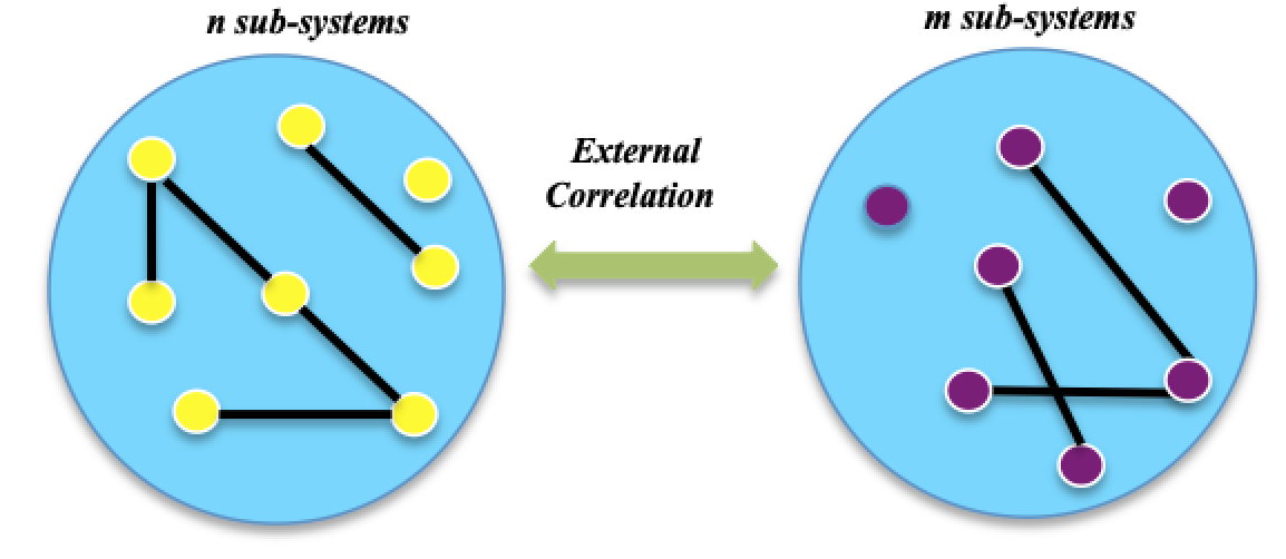
Figure 1: Schematic representation of the subsystems $n$ and $m$.

The index of correlation, whether applied to a complete $n+m$ system or to an individual component of the partition, returns a single number. If we fix the overall total correlation $I\left(N\right)$ to be some value, then this does not specify the state uniquely and there are many possible states of the complete system that will yield this value for the index of correlation. So if we have two density operators $\rho\left(1\right)$ and $\rho\left(2\right)$ that yield the same value for total index of correlation we have

$$I_{1}^{int}\left(\alpha\right)+I_{1}^{int}\left(\beta\right)+I_{1}^{ext}\left(\alpha,\beta\right)=I_{2}^{int}\left(\alpha\right)+I_{2}^{int}\left(\beta\right)+I_{2}^{ext}\left(\alpha,\beta\right)$$ (20)

or equivalently

$$\left[I_{1}^{int}\left(\alpha\right)+I_{1}^{int}\left(\beta\right)\right]-\left[I_{2}^{int}\left(\alpha\right)+I_{2}^{int}\left(\beta\right)\right]=I_{2}^{ext}\left(\alpha,\beta\right)-I_{1}^{ext}\left(\alpha,\beta\right)$$ (21)

Thus, for the same value of $I\left(N\right)$, increasing the degree of external correlation between the components of a given partition reduces the combined degree of internal correlation and vice versa. Indeed, if we consider a partition such that there is no external correlation between the 2 components then the density operator for the total system is separable and can be written in the form $\rho=\rho_{\alpha}\otimes\rho_{\beta}$.

3.2 Maximising the Total Correlation

Let us now consider states of the complete system such that the index of correlation for the complete system, $I\left(N\right)$, is maximised. This occurs when the total system is in a pure state. If we consider the sub-systems, $1,2,\ldots,N$ to be the same physical objects (thus $N$ electrons, or $N$ two-level atoms, for example) then the maximum value that $I\left(N\right)$ can take is just $I^{\max}\left(N\right)=NS^{\max}$ where $S^{\max}$ is the maximum entropy that a single sub-system can attain. For pure states of the complete system (whether maximally correlated or not) when we partition the space into just 2 components, the entropies of those components are equal. This follows from the Araki-Lieb triangle inequality which states that, for any two quantum systems $A$ and $B$, we have

$$\left|S_{A}-S_{B}\right|\leq S\leq S_{A}+S_{B}$$ (22)

For pure states of a system comprising of $N$ quantum systems, split into just 2 partitions of $n$ and $m$ objects we therefore have that

$$0 \leq I^{int}\left(\alpha\right)+I^{int}\left(\beta\right)\leq NS^{\max}$$

$$0 \leq I^{ext}\left(\alpha,\beta\right)\leq NS^{\max}$$ (23)

where if we maximise $I^{int}\left(\alpha\right)+I^{int}\left(\beta\right)$ we minimise $I^{ext}\left(\alpha,\beta\right)$, and vice versa.

In general, therefore, where the sub-systems are the same physical entities, in order to globally maximise the total correlation we require the following 2 conditions to be met

(i)

the total system must be in a pure state

(ii)

each individual sub-system must be in a state of maximum entropy so that the global maximum correlation strength is given by

$$I^{\max}\left(N\right)=\sum\limits_{k=1}^{N}\tilde{S}_{k}=NS^{\max}$$

In what follows we shall restrict ourselves to pure states of the total $N$-component system. With this condition we can view the total state as a purification of the $n$-component partition (or the $m$-component partition). As remarked above, the entropies of these two component partitions are equal if the total system is in a pure state.

4 Correlated Systems of $4$ Qubits

To begin with we shall consider $N=4$ so that we have just 4 qubits. This example is sufficient to illustrate many of the properties of the correlation between larger systems of qubits. We shall consider states of these 4 qubits that maximise $I\left(N\right)$ which, for 4 qubits, takes the value $4\ln 2$. Clearly, these states have to be pure states of 4 qubits. For 4 qubits there are only 2 possible $\left(n,m\right)$ partitions which are $\left(1,3\right)$ and $\left(2,2\right)$ and we consider the partitions $\left(3,1\right)$ and $\left(1,3\right)$ to be physically equivalent, by symmetry. Labelling the individual qubits as $a,b,c,d,\ldots$ it is clear from above that for a total state of $N$ qubits to maximise the information content of the correlations we must have that $S_{a}=S_{b}=S_{c}=\ldots=\ln 2$. Equivalently, we require that the reduced density operator for any single qubit to be of the form $\left(\left|0\right\rangle\left\langle 0\right|+\left|1\right\rangle\left\langle 1\right|\right)/2$.

4.1 Minimising $I^{ext}\left(\alpha,\beta\right)$

A state that (globally) maximises both $I\left(N\right)$ and $I^{int}\left(\alpha\right)+I^{int}\left(\beta\right)$ is not possible for the $\left(1,3\right)$ partition of 4 qubits. Such a state is, however, possible for the $\left(2,2\right)$ partition and an example of such a state is given by

$$\left|\psi\right\rangle_{S}=\frac{1}{\sqrt{2}}\left(\left|00\right\rangle_{ab}+\left|11\right\rangle_{ab}\right)\otimes\frac{1}{\sqrt{2}}\left(\left|00\right\rangle_{cd}+\left|11\right\rangle_{cd}\right)$$ (24)

where the states to the left of the tensor product in this expression refer to one component partition (containing the qubits labelled $a$ and $b$) and those to the right the other. This state minimises the external correlation between the chosen component partitions and is, thus, separable being a tensor product of two maximally correlated states of 2 qubits. It satisfies the constraint that the correlation of the total 4 qubit system is maximised.

It is important to note that, in general for a given $\left|\psi\right\rangle$ which maximises $I\left(N\right)$, the external correlation between partitions is invariant under permutations of particles within each component partition, but not invariant to permutations of particles between the partitions. As we shall see the GHZ state of $N$ qubits is a highly symmetric state in that the external correlation is invariant under permutations between partitions, and also invariant of the number of particles within each partition. The 4 qubit state (10) gives a nice example of the effect of permutation between the partitions. If we swap one particle from $\alpha$ with a particle from $\beta$ the resultant density operator is not separable in terms of the reduced density operators of the new $\alpha$ and $\beta$ components.

4.2 Maximising $I^{ext}\left(\alpha,\beta\right)$

An example of a state that (globally) maximises both $I\left(N\right)$ and $I^{ext}\left(\alpha,\beta\right)$ for the $\left(2,2\right)$ partition is given by

$$\left|\psi\right\rangle_{UE}=\frac{1}{2}\left(\left|00,00\right\rangle+\left|01,01\right\rangle+\left|10,10\right\rangle+\left|11,11\right\rangle\right)$$ (25)

where the comma in the state label distinguishes between the component partitions. If we label the individual qubits as $a,b,c,d$ and the two component partitions as $\alpha$ and $\beta$, so that the component partition $\alpha$ is comprised of the qubits $a$ and $b$, then it is easy to see that state (15) yields the reduced density operators

$$\rho_{\alpha\left(\beta\right)} =\frac{1}{2}\left(\left|00\right\rangle\left\langle 00\right|+\left|01\right\rangle\left\langle 01\right|+\left|10\right\rangle\left\langle 10\right|+\left|11\right\rangle\left\langle 11\right|\right)$$

$$\rho_{a\left(b\right)} =\frac{1}{2}\left(\left|0\right\rangle\left\langle 0\right|+\left|1\right\rangle\left\langle 1\right|\right)$$ (26)

It is clear that, given just one of the 2 component partitions, no evidence of correlation can be detected by any measurement. This is a general property of any state of $N$ systems that (globally) maximises the external correlation of a partition (for $N$ even this simply implies a partition such that $n=m=N/2$). This property is often expressed as a condition for ‘maximal’ entanglement in that this maximally ‘mixes’ the component systems.

4.3 Intermediate States

Now that we’ve seen examples of extremal states (maximally correlated states of 4 qubits that maximise the internal correlation, or the external correlation) we consider a state intermediate between these extremes. An obvious candidate is the GHZ state of 4 qubits, an example of which is given by

$$\left|\psi\right\rangle_{GHZ}=\frac{1}{\sqrt{2}}\left(\left|0000\right\rangle+\left|1111\right\rangle\right)$$ (27)

For this state the reduced density operators in the $\left(2,2\right)$ partition are given by

$$\rho_{\alpha(\beta)} =\frac{1}{2}\left(\left|00\right\rangle\left\langle 00\right|+\left|11\right\rangle\left\langle 11\right|\right)$$

$$\rho_{a(b)} =\frac{1}{2}\left(\left|0\right\rangle\left\langle 0\right|+\left|1\right\rangle\left\langle 1\right|\right)$$ (28)

The internal correlation of one component is, therefore, $I^{int}\left(\alpha\right)=\ln 2$ and the external correlation between the components is $I^{ext}\left(\alpha,\beta\right)=2\ln 2$. We can see that as we vary the state from $\left|\psi\right\rangle_{GHZ}$ to $\left|\psi\right\rangle_{S}$, whilst keeping $I\left(N\right)$ fixed at its maximum value of $4\ln 2$, we have that

$$\ln 2\leq I^{int}\left(\alpha\right)\leq 2\ln 2$$ (29)

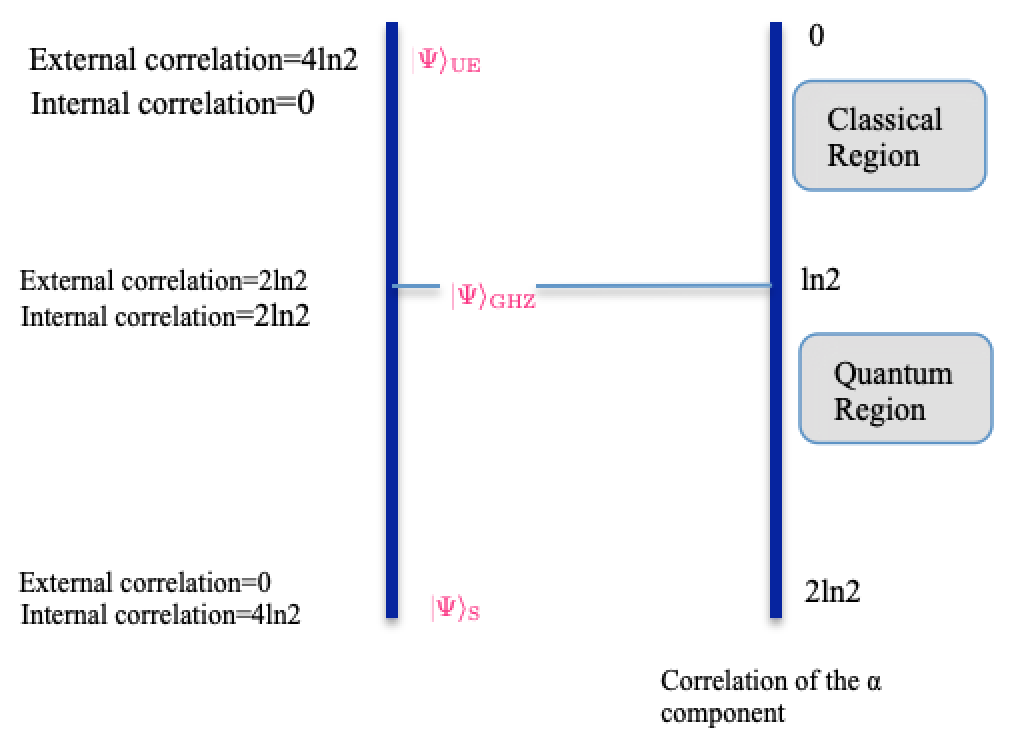
Figure 2: Schematic representation of the system and correlations considered.

but is this is precisely the non-classical region for the correlation of 2 qubits as expressed by (8). If we are given a 2-qubit component of a maximally correlated state of 4 qubits, then the GHZ state $\left|\psi\right\rangle_{GHZ}$ acts as a boundary between classical and quantum regions of the correlations for that component. This is summarized in the figure below. The states on the left hand side of this figure represent all possible purifications of 2 qubits, for the chosen partition, obtained by adding 2 extra qubits, that yield a maximally correlated pure state. In order to satisfy the requirement that this purification gives a maximally correlated state of 4 qubits we must have that

$$\rho_{a(b)}=\frac{1}{2}\left(\left|0\right\rangle\left\langle 0\right|+\left|1\right\rangle\left\langle 1\right|\right)$$ (30)

In the quantum regime for the correlations of 2 qubits we can see that a purification can be achieved by adding a single extra qubit. States of 2 qubits in this region can be purified by adding a single extra qubit giving a pure state of 3 qubits of the form

$$\left|\xi\right\rangle=\mu\left|0\right\rangle\otimes\left|\pi_{1}\right\rangle+\nu\left|1\right\rangle\otimes\left|\pi_{2}\right\rangle$$ (31)

which (except for the initial GHZ state at the boundary between the regions) is not a maximally correlated state of 3 qubits. Thus the states of 2 qubits, such that each individual qubit is in a maximally mixed state, which display non-classical correlation properties are precisely those that can be purified by the addition of a single qubit. In the classical regime for the correlations of 2 qubits we need at least 2 qubits to effect a purification, for the chosen partition. It seems reasonable to suppose that in this quantum region (where the 2 qubits originate from a maximally-correlated state of 4 qubits) we will obtain a violation of a suitably-chosen Bell inequality for the 2 qubits.

It should be noted that where the initial state is placed on the left hand side of figure 2 is dependent on which 2 qubits are chosen for the partition. If we begin with an initial state of the 4 qubits given by equation (15) then the above discussion assumes that qubits $a$ and $b$ were chosen for one partition and qubits $c$ and $d$ for the other. If, however, we choose the partitions $\left(a,c\right)$ and $\left(b,d\right)$ then, for these partitions, the external correlation is maximised whilst the internal correlation is zero.

5 Equal Partitions of Correlated Systems of $N$ Qubits

We now consider the effect of a single partition, as above, on systems of $N$ qubits. As we are going to consider a partitioning into 2 collections of equal numbers of qubits we shall take $N$ even so that $N=2n$ and label the qubits as $a_{1},a_{2},\ldots a_{2n}$. We consider pure states of the $2n$ qubits such that the entropy of any single qubit is $S\left(a_{k}\right)=\ln 2$ (that is, 1 bit) and that $I\left(N\right)=2n\ln 2$ (the pure state maximises the information content of the correlation for the entire system of $2n$ qubits). With these conditions we can write the internal and external correlations as

$$I^{ext}\left(\alpha,\beta\right) =2S\left(\alpha\right)$$

$$I^{int}\left(\alpha\right) =n\ln 2-S\left(\alpha\right)$$

$$I^{int}\left(\beta\right) =n\ln 2-S\left(\alpha\right)$$ (32)

As before, we can consider an ‘extremal’ state that maximises the external correlation which is

$$\left|\psi\right\rangle_{UE}=\frac{1}{\sqrt{2^{n}}}\sum\limits_{s}\left|s,s\right\rangle$$ (33)

where $s$ is an index, written in binary, such that $0\leq s\leq 2^{n}-1$ and the comma distinguishes the $\alpha$ and $\beta$ components. The index $s$ is just a bit string that ranges over the $2^{n}-1$ levels of the $\alpha$ and $\beta$ components. The internal correlations of the $\alpha$ and $\beta$ components.$I^{int}\left(\alpha\right)=I^{int}\left(\beta\right)=0$ for this state. As an example of the opposite extreme we can consider the state

$$\left|\psi\right\rangle_{S}=\frac{1}{\sqrt{2}}\left(\left|0\right\rangle^{n}+\left|1\right\rangle^{n}\right)\otimes\frac{1}{\sqrt{2}}\left(\left|0\right\rangle^{n}+\left|1\right\rangle^{n}\right)$$ (34)

which separates the $\alpha$ and $\beta$ components into two (maximally correlated) pure states. The state $\left|\psi\right\rangle_{S}$ maximises the internal correlations of the $\alpha$ and $\beta$ components but there is no external correlation and $I^{ext}\left(\alpha,\beta\right)=0$. As above we consider a GHZ state of the $2n$ qubits as an example of a state intermediate between these 2 extremes and this can be written as

$$\left|\psi\right\rangle_{GHZ}=\frac{1}{\sqrt{2}}\left(\left|0\right\rangle^{2n}+\left|1\right\rangle^{2n}\right)$$ (35)

The properties of internal and external correlations for these states are summarized in the figure below.

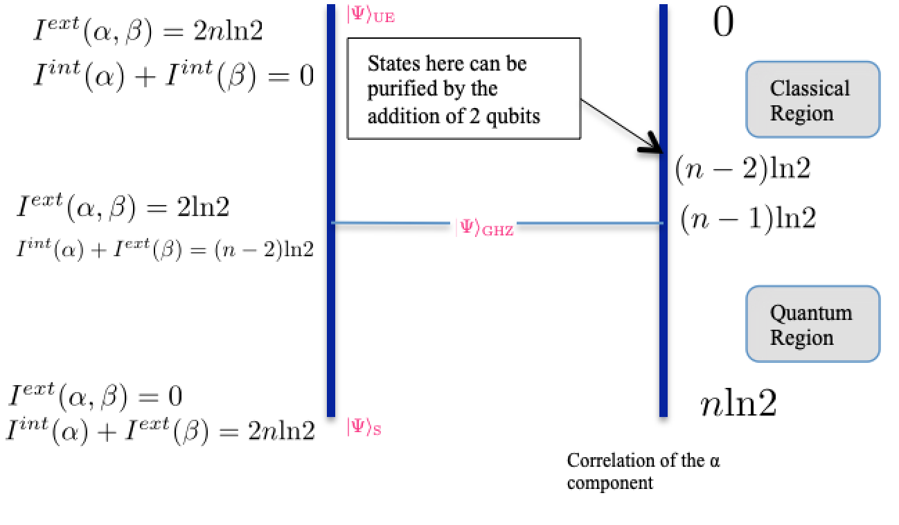
Figure 3: Schematic representation of the system and correlations considered.

The GHZ state again forms a kind of boundary between ‘classical’ and ‘quantum’. States of the $\alpha$-partition which yield $I^{int}\left(\alpha\right)$ in this quantum region are, necessarily, quantum mechanical in nature. States which yield $I^{int}\left(\alpha\right)$ in the ‘classical’ region may indeed display non-classical features, but in this region it is possible to find a classical state of the $n$ qubits with the same correlation strength. States of $n$ qubits, where each individual qubit has an entropy of $S\left(a_{k}\right)=\ln 2$, that can be purified by the addition of a single qubit, are in this quantum region. In the ‘classical’ region we need to add 2, or more, qubits to achieve a purification. The resultant purifications achieved are not maximally correlated states of $n+k$ qubits (where $k$ is the number of qubits we need to add to achieve purification), except for the case of the $n$-qubit $\alpha$ component that has arisen from the GHZ state of $2n$ qubits.

The GHZ state has a high degree of symmetry in the following sense. If we start with our $2n$ qubits prepared in the GHZ state and partition into $\left(n,m\right)$ qubits, then for this state the external correlation $I^{ext}\left(\alpha,\beta\right)=2\ln 2$, independently of where we make the cut or the number of qubits in each partition. The external correlation for the GHZ state is invariant under permutations of the particles in a given partition, and is invariant of the number of particles in each partition.

6 Conclusions

We have studied a measure of correlation strength for multipartite quantum systems, that is the information content of the correlation. It is important to emphasize that this is a measure of correlation strength only; it does not distinguish the precise nature of the correlation itself. However, we have shown that if this correlation strength is above a certain value then that can only be achieved by quantum mechanisms. This is defined as a natural extension of the index of correlation for bipartite systems. The index of correlation for two systems is just the quantum generalization of the classical mutual information and, for pure states, is equal to twice the entropy of entanglement. This information-based measure arises as a consequence of imposing certain natural conditions on any measure of correlation strength. In this note we have used this measure, together with the notion of partitioning, to derive some general properties of the correlation of interacting quantum systems. The term partitioning is only notional unless we take steps to physically create the partitions, but it allows us to identify the various entropy and correlation invariants of the interaction. Once these invariants have been identified it only requires very elementary techniques to establish these general properties.

6.1 Acknowledgments

BT greatly acknowledge supports from the Center for Cyber-Physical Systems (C2PS)-Khalifa University, Abu Dhabi, UAE.

References

- [1] Adesso, G., T. R. Bromley, and M. Cianciaruso. Measures and applications of quantum correlations. J. Phys. A Math. Theor. 2016, 49, 473001.
- [2] Horodecki, M., and J. Oppenheim. (Quantumness in the context of) Resource Theories. Int. J. Mod. Phys. B 2013 27, 1345019.
- [3] Modi, K., A. Brodutch, H. Cable, T. Paterek, and V. Vedral. The classical-quantum boundary for correlations: Discord and related measures. Rev. Mod. Phys. 2012, 84, 1655.
- [4] Postler, L.,Á. Rivas, P. Schindler, A. Erhard, R. Stricker, D. Nigg, T. Monz, R. Blatt, and M. Müller Experimental quantification of spatial correlations in quantum dynamics. Quantum 2018, 2, 90.
- [5] Ángel Rivas,, and M. Müller (2015), Quantifying spatial correlations of general quantum dynamics. New Journal of Physics 2015, 17(6), 062001.
- [6] Jacopo Trapani, Berihu Teklu, Stefano Olivares, and Matteo G. A. Paris Quantum phase communication channels in the presence of static and dynamical phase diffusion. Phys. Rev. A 2015, 92, 012317.
- [7] Berihu Teklu, Jacopo Trapani, Stefano Olivares, and Matteo G. A. Paris Noisy quantum phase communication channels. Phys. Scr. 2015, 90, 074027.
- [8] Hamza Adnane, Berihu Teklu, and Matteo G. A. Paris Quantum phase communication channels with non-deterministic noiseless amplifier. J. Opt. Soc. Am.B 2019, 36, 2938-2945.
- [9] A. Galindo, M.A. Martin-Delgado. Information and Computation: Classical and Quantum Aspects Rev.Mod.Phys. 2002, 74, 347-423.
- [10] Miguel A. Martin-Delgado. An Exclusion Principle for Sum-Free Quantum Numbers. https://arxiv.org/abs/2009.14491.
- [11] Nan Li and Shunlong Luo. Total versus quantum correlations in quantum states. Phys. Rev. A 2007, 26, 032327.
- [12] S. M. Barnett and S. J. D. Phoenix. Entropy as a measure of quantum optical correlation. Phys. Rev. A 1989, 40, 2404
- [13] S. M. Barnett and S. J. D. Phoenix, Information theory, squeezing, and quantum correlations. Phys. Rev. A 1991, 44, 535.
- [14] Adami and N. J. Cerf, von Neumann capacity of noisy quantum channels. Phys. Rev. A 1997, 56, 3470.
- [15] V. Vedral. The role of relative entropy in quantum information theory. Rev. Mod. Phys. 2002, 74, 197.
- [16] R. Horodecki, Informationally coherent quantum systems. Phys. Lett. A 1994, 187, 145.
- [17] A. K. Ekert. Quantum Cryptography Based on Bell’s Theorem. Phys. Rev. Lett. 1991, 67, 661.
- [18] Charles H. Bennett, Gilles Brassard, Claude Crepeau, Richard Jozsa, Asher Peres, and William K. Wootters. Teleporting an unknown quantum state via dual classical and Einstein-Podolsky-Rosen channels. Phys. Rev. Lett. 1993, 70, 1895.
- [19] R. F. Werner. Quantum states with Einstein-Podolsky-Rosen correlations admitting a hidden-variable model. Phys. Rev. A 1989, 40, 4277.
- [20] E. Knill and R. Laflamme. Power of One Bit of Quantum Information. Phys. Rev. Lett. 1998, 81, 5672.
- [21] S. L. Braunstein, C. M. Caves, R. Jozsa, N. Linden, S. Popescu, and R. Schack. Separability of Very Noisy Mixed States and Implications for NMR Quantum Computing. Phys. Rev. Lett. 1999, 83, 1054.
- [22] B. P. Lanyon, M. Barbieri, M. P. Almeida, and A. G. White. Experimental Quantum Computing without Entanglement. Phys. Rev. Lett. 2008, 101, 200501.
- [23] L. Henderson and V. Vedral. Classical, quantum and total correlations. J. Phys. A: Math. Gen. 2001, 34, 6899.
- [24] H. Ollivier and W. H. Zurek. Quantum Discord: A Measure of the Quantumness of Correlations. Phys. Rev. Lett. 2001, 88, 017901. The classical-quantum boundary for correlations: Discord and related measures. Rev. Mod. Phys. 2012 84, 1655.
- [25] A. Misra, A. Biswas, A. K. Pati, A. Sen(De), and U. Sen. Quantum correlation with sandwiched relative entropies: Advantageous as order parameter in quantum phase transitions. Phys. Rev. E 2015, 91, 052125.
- [26] J. Maziero, L. C. Celeri, R. M. Serra, V. Vedral. Classical and quantum correlations under decoherence. Phys. Rev. A 2009, 80, 044102
- [27] J. Maziero, H. C. Guzman, L. C. Celeri, M. S. Sarandy, and R. M. Serra. Quantum and classical thermal correlations in the spin- chain. Phys. Rev. A 2010 , 82, 012106.
- [28] R. Auccaise, J. Maziero, L. C. Celeri, D. O. Soares-Pinto, E. R. deAzevedo, T. J. Bonagamba, R. S. Sarthour, I. S. Oliveira, and R. M. Serra. Experimentally Witnessing the Quantumness of Correlations. Phys. Rev. Lett. 2011 , 107, 070501.
- [29] R. Auccaise, L. C. Celeri, D. O. Soares-Pinto, E. R. deAzevedo, J. Maziero, A. M. Souza, T. J. Bonagamba, R. S. Sarthour, I. S. Oliveira, and R. M. Serra Environment-Induced Sudden Transition in Quantum Discord Dynamics Phys. Rev. Lett. 2011 , 107, 140403 .
- [30] J. Maziero, L. C. Celeri, R. M Serra, M. S Sarandy. Long-range quantum discord in critical spin systems. Physics Letters A 2012 , 18, 1540-1544.
- [31] M. Horodecki, P. Horodecki, R. Horodecki, J. Oppenheim, A. Sen, U. Sen, and B. Synak-Radtke. Local versus nonlocal information in quantum-information theory: Formalism and phenomena. Phys. Rev. A 2005, 71, 062307.
- [32] A. Datta, A. Shaji, and C. M. Caves. Quantum Discord and the Power of One Qubit. Phys. Rev. Lett. 2008, 100, 050502.
- [33] V. Madkok and A. Datta. Quantum discord as a resource in quantum communication. Int. J. Mod. Phys. B 2013, 27, 1345041.
- [34] A. Ferraro and M. G. A. Paris. Nonclassicality Criteria from Phase-Space Representations and Information-Theoretical Constraints Are Maximally Inequivalent. Phys. Rev. Lett. 2012, 108, 260403.
- [35] T. J. Osborne and F. Verstraete. General monogamy in-equality for bipartite qubit entanglement Phys. Rev. Lett. 2006 96, 220503.
- [36] G. Adesso and F. Illuminati. Continuous variable tangle, monogamy inequality, and entanglement sharing in Gaussian states of continuous variable systems New J. Phys. 2006 8, 15.
- [37] Hiroshima, G. Adesso, and F. Illuminati. Monogamy in-equality for distributed Gaussian entanglement Phys. Rev. Lett. 2007 98, 050503.
- [38] M. Koashi and A. Winter. Monogamy of quantum entanglement and other correlations, Phys. Rev. A 2004, 69, 022309.
- [39] Y.-C. Ou and H. Fan. Monogamy inequality in terms of negativity for three-qubit states Phys. Rev. A 2007 75, 062308.
- [40] J. S. Kim. Negativity and tight constraints of multiqubit entanglement. Phys. Rev. A 2018 97, 012334.
- [41] S. M. Barnett and S. J. D. Phoenix. Information-Theoretic limits to Quantum Cryptography. Phys. Rev. A 1993, 48, R5.
- [42] F Herbut. On mutual information in multipartite quantum states and equality in strong subadditivity of entropy. J. Phys. A: Math. Gen. 2004 37, 3535.
- [43] Jonas Maziero. Distribution of Mutual Information in Multipartite States. Braz. J. Phys. 2014 44, 194.