Complementary probe of dark matter blind spots by lepton colliders and gravitational waves

Abstract

We study how to unravel the dark matter blind spots by phase transition gravitational waves in synergy with collider signatures at electroweak one-loop level taking the inert doublet model as an example. We perform a detailed Monte Carlo study at the future lepton colliders in the favored parameter space, which is consistent with current dark matter experiments and collider constraints. Our studies demonstrate that the Circular Electron Positron Collider and other future lepton colliders have the potential to explore the dark matter blind spots.

I Introduction

In recent years, there is a growing number of cosmological and astrophysical evidence on the existence of the mysterious dark matter (DM) including the galaxy rotation curve, the precise cosmic microwave background spectrum, the bullet cluster collision, the gravitational lensing effects, and so on Bertone and Hooper (2018). However, the absence of DM signals at the DM direct search and LHC has almost pushed DM parameter space to the blind spots, where the coupling between DM and the standard model (SM) particles is too small to be detected directly in the DM detectors. This situation may point us towards some new approaches to explore these DM parameter spaces, such as the future gravitational wave (GW) experiments and the future lepton colliders. After the discovery of GW by LIGO, GW becomes a novel and realistic approach to understand and explore the fundamental physics, including the mysterious DM. Meanwhile, the proposed future lepton colliders may also help to unravel the DM nature due to their clean backgrounds and high sensitivity.

In this work, we revise the well-studied inert doublet model (IDM) Barbieri et al. (2006), which can provide natural DM candidates Barbieri et al. (2006); Lopez Honorez and Yaguna (2010). The current DM direct search has constrained the Higgs-DM coupling to be very small. The DM direct search might be difficult to observe the possible DM signals. However, the inert scalars including the DM could trigger a strong first-order phase transition (SFOPT) and produce the phase transition GWs. Meanwhile, they could modify the Higgs-Z boson coupling and the triple Higgs coupling through loop effects. These modifications could be exploited by the precise measurements of the process $e^{+}e^{-}\to hZ$ with its various decay channels at future lepton colliders, such as Circular Electron Positron Collider (CEPC) Dong et al. (2018); An et al. (2019), Future Circular Collider (FCC-ee) Abada et al. (2019), and International Linear Collider (ILC) Fujii et al. (2017). In this work, we focus on the detailed Monte Carlo (MC) simulations of the lepton collider signals up to one-loop level in complement to the corresponding GW signals induced by this DM model. The details of SFOPT and collider simulations are given in the Appendixes A and B.

The work is organized as the following: In section II, we review the IDM, the DM blind spots from various constraints and the condition of a SFOPT. The detailed discussions of the phase transition GW spectra are given in section III. Then we focus on the MC simulations of the signals at future lepton colliders at the one-loop level in section IV. Lastly, the conclusion is given in section V.

II Dark matter and strong first-order phase transition in the inert doublet model

The well-studied IDM could provide a natural DM candidate and improve the naturalness Barbieri et al. (2006); Lopez Honorez and Yaguna (2010). This model could also produce a SFOPT Chowdhury et al. (2012). The tree-level scalar potential at zero temperature of the IDM can be written as the following:

$$V= \mu^{2}_{1}|\Phi|^{2}+\mu^{2}_{2}|\eta|^{2}+\frac{1}{2}\lambda_{1}|\Phi|^{4}+\frac{1}{2}\lambda_{2}|\eta|^{4}$$

$$+\lambda_{3}|\Phi|^{2}|\eta|^{2}+\lambda_{4}|\Phi^{\dagger}\eta|^{2}+\frac{1}{2}\{\lambda_{5}(\Phi^{\dagger}\eta)^{2}+h.c.\}\,\,,$$ (1)

where $\Phi$ is the SM Higgs doublet and $\eta$ is the inert doublet. The vacuum stability puts the conditions Barbieri et al. (2006); Lopez Honorez and Yaguna (2010)

$$\lambda_{1}>0,\ \lambda_{2}>0,\ \sqrt{\lambda_{1}+\lambda_{2}}+\lambda_{3}>0,\ \lambda_{3}+\lambda_{4}\pm|\lambda_{5}|>0\,\,.$$ (2)

At zero temperature, the two doublet scalar fields can be expanded as

$$\Phi=\begin{pmatrix}G^{+}\\ \frac{1}{\sqrt{2}}(h+v+iG^{0})\end{pmatrix},\ \eta=\begin{pmatrix}H^{+}\\ \frac{1}{\sqrt{2}}(H+iA)\end{pmatrix},$$ (3)

where SM Higgs boson $h$ has 125 GeV mass and the vacuum expectation value (VEV) $v=246$ GeV. $G^{+}$ and $G^{0}$ are the Nambu-Goldstone bosons. At zero temperature, the scalar masses can be obtained as

$$m_{h}^{2} =\lambda_{1}v^{2},$$ (4)

$$m_{H}^{2} =\mu_{2}^{2}+\frac{1}{2}(\lambda_{3}+\lambda_{4}+\lambda_{5})v^{2},$$ (5)

$$m_{A}^{2} =\mu_{2}^{2}+\frac{1}{2}(\lambda_{3}+\lambda_{4}-\lambda_{5})v^{2},$$ (6)

$$m^{2}_{H^{\pm}} =\mu_{2}^{2}+\frac{1}{2}\lambda_{3}v^{2}\,\,.$$ (7)

These new inert scalars could contribute to the modification of the $T$ parameter $\Delta T$, which could be approximated as

$$\Delta T\simeq\frac{1}{6\pi e^{2}v^{2}}(m_{H^{\pm}}-m_{H})(m_{H^{\pm}}-m_{A})\,\,.$$ (8)

If $m_{A}^{2}=m^{2}_{H^{\pm}}$ or $m_{H}^{2}=m^{2}_{H^{\pm}}$, $\Delta T\simeq 0$. A simple and natural way to avoid large $T$ parameter deviation $\Delta T$ is to assume $m_{A}^{2}=m^{2}_{H^{\pm}}$. To satisfy this condition, one assumes

$$\lambda_{4}=\lambda_{5}<0,~{}~{}\lambda_{3}>0\,\,,$$ (9)

which would be consistent with all the constraints from electroweak precise measurements, DM direct searches and the collider data. The T parameter constraint does not require the signs of these couplings. Thus, the choices of these signs are just for simplicity and for the constraints from the DM direct searches and the collider data, as in Ref. Chowdhury et al. (2012). Therefore, we have degenerated pseudoscalar and charged scalar masses

$$m_{A}^{2}=m^{2}_{H^{\pm}}=\mu_{2}^{2}+\frac{1}{2}\lambda_{3}v^{2}\,\,.$$ (10)

Under the above assumptions, the particle $H$ ($m_{H}^{2}=\mu_{2}^{2}+\lambda_{L}v^{2}$) is the lightest particle and can be the natural DM candidate Barbieri et al. (2006); Lopez Honorez and Yaguna (2010). And the DM-Higgs boson coupling is defined as $\lambda_{L}=(\lambda_{3}+\lambda_{4}+\lambda_{5})/2$. The loop correction does not change our results since $\Delta T$ is very small by assuming $m_{A}^{2}=m^{2}_{H^{\pm}}$. And DM constraint has a slight modification after including the loop correction.

However, the DM direct search has put strong constraints on this DM-Higgs coupling for different DM masses. For example, the XENON1T data have pushed the DM-nucleon spin-independent elastic scatter cross section up to $\sigma_{\text{SI}}=4.1\times 10^{-47}~{}\text{cm}^{2}$ for about 30 GeV DM mass at $90\%$ confidence level Aprile et al. (2018). These constraints almost reach the blind spots of the IDM, which means the DM-Higgs coupling $\lambda_{L}$ should be extremely small. The favored channel is the Higgs funnel region, where the DM mass is about half of the Higgs boson mass ($m_{H}\simeq m_{h}/2$). For this Higgs funnel region, we can estimate the cross section as

$$\sigma_{\rm SI}\simeq\frac{\lambda_{L}^{2}f_{N}^{2}}{\pi}\left(\frac{m_{N}^{2}}{m_{H}m_{h}^{2}}\right)^{2}$$ (11)

with $f_{N}\simeq 0.3$. Here, we first do some simple estimations using the above equation to get the constraint of DM-Higgs coupling from the DM direct search. Here and after, we use $\sc{micrOMEGAs}$ Barducci et al. (2018) to do the precise calculations. We show the constraint below

$$\lambda_{L}\lesssim 0.003\,\,.$$ (12)

These blind spots are difficult for future direct observation of DM signal at DM direct search experiments. In this work, we study how to use future lepton colliders in synergy with GW to explore the DM blind spots. The corresponding DM relic abundance for the blind spots of the Higgs funnel region should satisfy the Plank 2018 result Aghanim et al. (2018):

$$\Omega_{\text{DM}}h^{2}=0.11933\pm 0.00091\,\,.$$ (13)

Since the DM mass is about half of the Higgs mass, the dominant DM annihilation process is the Higgs-mediated $s$ channel $HH\to h\to W^{\pm*}W^{\mp}$ with off-shell $W$ boson, namely, the ratio of the channel’s contribution is about $52\%$. The second important channel is the $HH\to h\to b\bar{b}$ with the contribution about $32\%$. We use the $\sc{micrOMEGAs}$ Barducci et al. (2018) to precisely calculate the DM relic abundance including the important resonant effects.

Besides the still allowed DM candidate in the blind spots, the IDM in the blind spots could also trigger a SFOPT, which can further produce phase transition GW signals, and have a possibility to explain the electroweak baryogenesis. When $\lambda_{3}$, $\lambda_{4}$, $\lambda_{5}$ are $\mathcal{O}(1)$, a SFOPT can be triggered Chowdhury et al. (2012); Borah and Cline (2012); Gil et al. (2012); Cline and Kainulainen (2013); AbdusSalam and Chowdhury (2014); Blinov et al. (2015); Cao et al. (2018); Huang and Yu (2018); Laine et al. (2017); Senaha (2019); Huang and Senaha (2019); Kainulainen et al. (2019). The subtle point is the cancellation between the three couplings, which can make the DM-Higgs coupling very small to satisfy the DM direct search. We show the detailed discussions of the phase transition in Appendix A.

Numerically, we use the package $\sc{micrOMEGAs}$ Barducci et al. (2018) to consider all the precise constraints from DM relic abundance $\Omega_{\text{DM}}h^{2}$, DM direct search $\sigma_{\text{SI}}$, collider constraints Belyaev et al. (2018), and use $\sc{CosmoTransitions}$ Wainwright (2012) to calculate the phase transition dynamics. Taking all the above discussions into consideration, we choose the following benchmark point $m_{h}=125$ GeV $m_{A}=m_{H^{\pm}}=300$ GeV, $m_{H}=62.66$ GeV, $\mu_{2}=61.69$ GeV, which corresponds to $\lambda_{L}=(m_{H}^{2}-\mu_{2}^{2})/v^{2}=0.002$. This benchmark point set can explain the whole DM and satisfy the DM direct search. Taking this set of benchmark points, the relic density, DM direct search, collider constraints and a SFOPT can be satisfied simultaneously.

III Gravitational wave spectra

There are three well-known sources to produce phase transition GWs during a SFOPT, namely, sound wave, turbulence and bubble wall collisions. For most particle physics models beyond the SM, the dominant source is the sound wave mechanism, which usually produces more significant and long-lasting signal Hindmarsh et al. (2014, 2015, 2017) compared to turbulence and bubble wall collisions. To obtain the GW spectra, we need to calculate the phase transition dynamics, which is quantified by several phase transition parameters. We can calculate these parameters from the finite-temperature effective potential $V_{\rm eff}$, which is given in the appendix A. The first parameter is the phase transition strength parameter $\alpha$. There are several different definitions of $\alpha$, and we use the conventional definition below

$$\alpha=\frac{\Delta V_{\rm eff}-T\frac{\partial\Delta V_{\rm eff}}{\partial T}}{\rho_{R}}\,\,,$$ (14)

where $\rho_{R}=\pi^{2}g_{\rm eff}T_{+}^{4}/30$. $T_{+}$ should be the temperature of the plasma surrounding the bubbles where GWs have been produced. It is important to choose the correct $T_{+}$ Wang et al. (2020a), which is usually chosen as the nucleation temperature $T_{n}$ (At $T_{n}$, one bubble is nucleated in one Hubble radius.) or the percolation temperature $T_{p}$ (At $T_{p}$, about $34\%$ of false vacuum has been converted to true vacuum and a large numbers of bubbles have collided and percolated.). The phase transition strength parameters calculated at the nucleation temperature $T_{n}$ and the percolation temperature $T_{p}$ are denoted by $\alpha_{n}$ and $\alpha_{p}$, respectively. The second parameter is the mean bubble separation $R_{*}$, which is given by

$$R_{*}=n_{b}^{-1/3}\,\,,$$ (15)

where $n_{b}$ is the bubble number density Turner et al. (1992).

From the recent numerical simulations Hindmarsh et al. (2014, 2015, 2017), the simulated GW spectrum from the sound wave can be written as

$$h^{2}\Omega_{\rm sw}(f)\simeq 1.64\times 10^{-6}(H_{*}\tau_{\rm sw})(H_{*}R_{*})K^{2}\left(\frac{100}{g_{*}}\right)^{1/3}(f/f_{\rm sw})^{3}\left(\frac{7}{4+3(f/f_{\rm sw})^{2}}\right)^{7/2},$$ (16)

with the peak frequency

$$f_{\rm sw}\simeq 2.6\times 10^{-5}~{}\text{Hz}\frac{1}{H_{*}R_{*}}\left(\frac{T_{*}}{100~{}\rm GeV}\right)\left(\frac{g_{*}}{100}\right)^{1/6}\,\,.$$ (17)

$\tau_{\rm sw}$ is the sound wave duration time,

$$\tau_{\rm sw}=\min\left[\frac{1}{H_{*}},\frac{R_{*}}{\overline{U}_{f}}\right]\,\,,$$ (18)

and the kinetic energy fraction

$$K=\frac{\kappa_{v}\alpha}{1+\alpha}\,\,.$$ (19)

$H_{*}$ is the Hubble parameter at $T_{*}$. The efficiency parameter $\kappa_{v}$ is the fraction of vacuum energy converted into the fluid bulk kinetic energy. The root-mean-square fluid velocity $\overline{U}_{f}^{2}$ is approximated as Hindmarsh et al. (2017); Caprini et al. (2020); Ellis et al. (2019)

$$\overline{U}_{f}^{2}\approx\frac{3}{4}K\,\,.$$ (20)

The duration time $\tau_{\rm sw}$ determines whether the sound wave spectrum is suppressed or not. Qualitatively, for $H_{*}\tau_{\rm sw}<1$, the GW spectrum is suppressed by a factor of $H_{*}R_{*}/\overline{U}_{f}$, namely, $\Omega_{\rm sw}\propto K^{3/2}$. In the opposite direction, there is no suppression, and the GW spectrum scales as $\Omega_{\rm sw}\propto K^{2}$.

Many models predict the suppressed sound wave spectrum, and hence the contributions from turbulence and bubble collisions might not be negligible. The GW spectrum from turbulence is still controversial Kosowsky et al. (2002); Gogoberidze et al. (2007); Niksa et al. (2018); Caprini et al. (2020) and we use the following formula as an estimation Caprini et al. (2009, 2016):

$$h^{2}\Omega_{\rm turb}(f)\simeq 1.14\times 10^{-4}H_{*}R_{*}\left(\frac{\kappa_{\rm turb}\alpha}{1+\alpha}\right)^{3/2}\left(\frac{100}{g_{*}}\right)^{1/3}\frac{(f/f_{\rm turb})^{3}}{(1+f/f_{\rm turb})^{11/3}(1+8\pi f/H_{*})}\,\,.$$ (21)

The efficiency factor $\kappa_{\rm turb}$ is given by the recent simulations Hindmarsh et al. (2015). The Hubble rate at $T_{*}$ is given by

$$H_{*}=1.65\times 10^{-5}~{}\text{Hz}\left(\frac{T_{*}}{100~{}\rm GeV}\right)\left(\frac{g_{*}}{100}\right)^{1/6}\,\,.$$ (22)

Thus, we can obtain the peak frequency of turbulence $f_{\rm turb}$

$$f_{\rm turb}\simeq 7.91\times 10^{-5}~{}\text{Hz}\frac{1}{H_{*}R_{*}}\left(\frac{T_{*}}{100~{}\rm GeV}\right)\left(\frac{g_{*}}{100}\right)^{1/6}.$$ (23)

To obtain more reliable GW spectra, we need to first know the bubble wall velocity and energy budget which are explicitly model dependent. The GW spectra strongly depend on the bubble wall velocity. Most of the previous studies on the GW spectra in a given new physics model just take the bubble wall velocity as an input parameter. Explicitly, the bubble wall velocity is determined by the friction force of thermal plasma acting on the bubble wall. The friction force is further determined by the deviation of massive particle populations from the thermal equilibrium. Here, we estimate a more realistic bubble wall velocity as $v_{b}=0.3$ based on the Refs. Moore and Prokopec (1995); Wang et al. (2020b), where the friction force is similar to the SM case. The precise calculations of the bubble wall velocity for a given new physics model are complicated, which is beyond the scope of this paper. We notice that this model is similar to the model discussed in Refs. Moore and Prokopec (1995); Wang et al. (2020b), and hence choose the approximated values as in these references. This bubble wall velocity is smaller than the sound speed $v_{s}=\sqrt{3}/3$, and thus this case belongs to the deflagration mode, which can be further used to successfully explain the electroweak baryogenesis. For the energy budget, the model-independent formula is used in most of the previous studies. The model-dependent studies find that there are modifications of the energy budget considering more realistic sound speed in the broken phase and symmetric phase during a SFOPT Giese et al. (2021); Wang et al. (2021). However, the phase transition strength is weak and the corresponding correction of the energy budget is not significant in this work Giese et al. (2021); Wang et al. (2021). We can still use the model-independent energy budget formula as an estimation.

We could first give some qualitative discussions on our predictions of the GW spectra. In our previous work Wang et al. (2020a), we classified the SFOPT into four cases. This model belongs to the weakest type, namely, the slight supercooling, which corresponds to $\alpha_{p}\leq 0.1$. In this case, $\alpha_{n}$ can be a good approximation to $\alpha_{p}$ since $\alpha_{p}-\alpha_{n}\ll 0.1$. For slight supercooling, the GW signal is too weak and difficult to be detected by the Laser Interferometer Space Antenna (LISA) Caprini et al. (2020). The signal may be within the sensitivity of Ultimate-Decihertz Interferometer Gravitational wave Observatory (U-DECIGO) Kudoh et al. (2006), and big bang observer (BBO) Corbin and Cornish (2006).

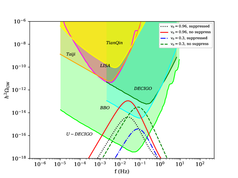
Figure 1: The GW spectra for IDM. The colored regions represent the expected sensitivities of the future GW experiments. Different lines depict different GW spectra for different bubble wall velocities and sound wave duration.

Combining the above discussions, we show the GW spectra from the three sources in Fig. 1 for the benchmark points. The colored regions represent the expected sensitivity for the future GW experiments, LISA Amaro-Seoane et al. (2017); Caprini et al. (2016, 2020); LIS , TianQin Luo et al. (2016); Hu et al. (2018); Mei et al. (2020), Taiji Hu and Wu (2017); Ruan et al. (2020), DECIGO Seto et al. (2001); Kawamura et al. (2011), U-DECIGO Kudoh et al. (2006), and BBO Corbin and Cornish (2006). The red line represents the GW spectra for the bubble wall velocity $v_{b}=0.96$ without suppression, while the black dotted line depicts the GW spectra for the bubble wall velocity $v_{b}=0.96$ with suppression. The blue dash-dotted line and the green dashed line corresponds to the GW spectra with and without suppression for the wall velocity $v_{b}=0.3$, respectively. It is obvious that the bubble wall velocity and suppression effects are significant. For our benchmark points in the IDM, our estimation favors the wall velocity $v_{b}=0.3$ with suppression effect. Since this type belongs to the slight supercooling case, the GW spectra are too weak to be detected by LISA, Taiji, TianQin, and DECIGO. However, they can reach the sensitivity of U-DECIGO or BBO.

After having the GW spectra of the signal, the detectability of the GW signal needs to be quantified by defining the conventional signal-to-noise ratio (SNR):

$$\text{SNR}=\sqrt{\mathcal{T}_{\text{obs}}\int_{f_{\text{min}}}^{f_{\text{max}}}\mathrm{d}f\left[\frac{h^{2}\Omega_{\text{GW}}(f)}{h^{2}\Omega_{\text{det}}(f)}\right]^{2}}\,,$$ (24)

where $\mathcal{T}_{\text{obs}}$ is the total observation time and $h^{2}\Omega_{\text{det}}(f)$ is the nominal sensitivity of a given GW experiment configuration to cosmological sources. We simply assume four-years mission duration time with a duty cycle of 75% $\mathcal{T}_{\text{obs}}$, and take $\mathcal{T}_{\text{obs}}\simeq 9.46\times 10^{7}\,$s, which is guaranteed by the LISA LIS . For the benchmark points with the wall velocity $v_{b}=0.3$ and the suppression effect, the SNR is about nine. We can see that U-DECIGO is capable to detect the signals with enough observation time.

It is worth noticing that there are large theoretical uncertainties in the predictions of the GW spectra. In the above discussions, we clarify the dominant uncertainties from model-dependent bubble wall velocity, definition of the phase transition parameters, the suppression effects in sound wave Guo et al. (2021), model-dependent kinetic energy fraction, and so on. In Fig. 1, we choose more conservative estimations in our calculations. Considering the large uncertainties and taking progressive estimations, the GW signal could be within the sensitivity of DECIGO and the marginal region of LISA. In a recent study Croon et al. (2020), the three-dimensional approach could significantly reduce the uncertainties. We leave the three-dimension study for this IDM in our future work.

IV Precise predictions at future lepton colliders

The SM $hZ$ leading-order cross section ($e^{+}e^{-}\to hZ\to\mu^{+}\mu^{-}h$) at 240 GeV CEPC is 6.77 fb calculated by $\sc{Whizard~{}1.95}$ Kilian et al. (2011). At the lepton collider, the Higgs-strahlung process offers an unique opportunity for a model-independent precise measurement of the $hZZ$ coupling strength. At the CEPC Dong et al. (2018); An et al. (2019) with an integrated luminosity of $5.6~{}\mathrm{ab}^{-1}$, the precision of $\sigma_{hZ}$ could achieve about $0.5\%$ with a ten-parameter fit to the CEPC and high luminosity LHC (HL-LHC) data An et al. (2019), which corresponds to the uncertainty of $hZZ$ coupling 0.25%. The uncertainty could further reach 0.12% with a seven-parameter effective field theory (EFT) fit De Blas et al. (2019). At the ILC, the projected uncertainty of $hZZ$ coupling for the ILC EFT analysis could reach 0.18% when combining HL-LHC, 250 GeV ILC and 500 GeV ILC data Bambade et al. (2019). At the FCC-ee, combining HL-LHC, 240 GeV and 365 GeV FCC-ee data, the $hZZ$ uncertainty also reach 0.16%. The above measurements are all based on the recoil mass technique to give model-independent constraints, where the $Z$ boson decays to $e^{+}e^{-}$, $\mu^{+}\mu^{-}$ or $q\bar{q}$ and the Higgs boson decay final states do not need to be considered. In a specific model, when the Higgs decay mode could be determined, the $hZZ$ coupling could be measured more precisely.

Due to the loop effects of the new particles, the $hZZ$ coupling strength is modified in the IDM. The one-loop electroweak corrections of the $hZZ$ vertex in the IDM are calculated in Arhrib et al. (2015); Kanemura et al. (2016). In this study, we adopt the one-loop electroweak corrections in the Ref. Kanemura et al. (2016). After considering the one-loop electroweak radiative effects, the Lorentz structures of the $hZZ$ coupling become Barklow et al. (2018):

$$\mathcal{L}_{hZZ}=M^{2}_{Z}(\frac{1}{v}+\frac{a_{Z}}{2\Lambda})Z_{\mu}Z^{\nu}h+\frac{b_{Z}}{2\Lambda}Z_{\mu\nu}Z^{\mu\nu}h+\frac{\tilde{b}_{Z}}{2\Lambda}{Z}_{\mu\nu}\tilde{Z}^{\mu\nu}h\,\,,$$ (25)

where $Z_{\mu\nu}\equiv\partial_{\mu}Z_{\nu}-\partial_{\nu}Z_{\mu}$ and $\tilde{Z}_{\mu\nu}\equiv\frac{1}{2}\epsilon_{\mu\nu\rho\sigma}Z^{\rho\sigma}$. The detailed expressions of $a_{Z}$, $b_{Z}$, $\tilde{b}_{Z}$ can be found in Ref. Kanemura et al. (2016). The first term is similar to the SM and will affect the total cross section, while the second and the third term will affect final state angular distributions as well as the total cross sections.

We integrate the next-leading-order (NLO) electroweak correction of the $hZZ$ vertex in the $e^{+}e^{-}\to\mu^{+}\mu^{-}h$ process in the SM as well as in the IDM into the $\sc{Whizard}$ code. The $hZ$ cross sections with the one-loop contributions to the $hZZ$ coupling at the different center-of-mass energy are listed in Table. 1. The deviation of the $e^{+}e^{-}\to\mu^{+}\mu^{-}h$ NLO cross section between the IDM and the SM is defined as:

$$\Delta\sigma\equiv(\sigma_{IDM}^{NLO}-\sigma_{SM}^{NLO})/\sigma_{SM}^{NLO},$$ (26)

where $\sigma_{IDM}^{NLO}$ and $\sigma_{SM}^{NLO}$ are the cross sections with the electroweak one-loop contributions of the $hZZ$ coupling in the IDM and in the SM. $\Delta\sigma$ is about $-0.2\%$ within our benchmark parameters at the 240 GeV. Although the deviation is slight, it still can be searched at the future electron-positron colliders with the model-independent measurements. It is worth noting that the deviation depends on the beam polarization, $\Delta\sigma$ reaches the minimum for the pure left-hand electron and right-hand positron, where ILC could play an important role.

Table 1: The electroweak one-loop cross sections for the $e^{+}e^{-}\to\mu^{+}\mu^{-}h$ process in the SM model and the IDM model when the center-of-mass energies are 240 GeV and 250 GeV. The parameters are $m_{h}=125$ GeV, $m_{A}=m_{H^{\pm}}=300$ GeV, $m_{H}=62.66$ GeV, $\mu_{2}=61.69$ GeV.

$240$ GeV	total $\sigma$	$e^{-}_{L}e^{+}_{R}$	$e^{-}_{R}e^{+}_{L}$
SM NLO (fb)	6.244	15.203	9.749
IDM NLO (fb)	6.230	15.159	9.750
$\Delta\sigma$	-0.22%	-0.289%	0%
$250$ GeV
SM NLO (fb)	6.615	16.158	10.376
IDM NLO (fb)	6.623	16.126	10.375
$\Delta\sigma$	-0.12%	-0.20%	0%

Furthermore, considering that in the above future collider predictions, the common procedure is first to measure the $hZ$ production cross section and the $hZZ$ coupling by the model-independent measurement of the Higgs decay final states with the recoil mass technique. Then, measure the branching ratios of each Higgs decay channel. The precision is sacrificed for the model independence. However, since the deviation of the $hZ$ production cross section in the IDM and SM is very small, it is hard to be distinguished with the above model-independent measurements in those future colliders. In order to suppress the background and increase the measurement significance, we could directly measure the $e^{+}e^{-}\to Zh\to l^{+}l^{-}b\bar{b}$ process to suppress the backgrounds with the explicit Higgs decay channel $h\to b\bar{b}$, because in our scenario the Higgs boson decay is considered the same as the SM Higgs. Then, the result will be folded back to the $hZ$ cross section with the SM $h\to b\bar{b}$ branching ration. In this case, a lot of backgrounds in the model-independent analysis will be exceedingly suppressed, such as two fermion production ($e^{+}e^{-}\to l^{+}l^{-}$), as well as four leptonic fermion production $e^{+}e^{-}\to ZZ/WW\to llll(ll\nu\nu)$ and so on. Thus, the $hZZ$ coupling measurement resolution will increase, comparing with the above predictions in the future colliders. Because we cannot fully simulate the future collider MC analysis, we will perform the fast simulation, analyze with the explicit $h\to b\bar{b}$ model measurement and recoil mass measurement, respectively. As a comparison, the model-independent measurement for the $hZZ$ coupling is listed in the Appendix B. By comparing two results, we can estimate the $hZZ$ constraints with the full simulation in the future collider. It will be clear that the ability to search the anomalous $hZZ$ coupling at the future Higgs factories will be more greatly enhanced than the above $\Delta hZZ$ uncertainties with the model independent method.

We will perform the search for $e^{+}e^{-}\to Zh\to l^{+}l^{-}b\bar{b}$ in the following section and state the recoil mass results in the Appendix B to show the possible measurement accuracy. By comparing two methods, we will understand how much the $\Delta hZZ$ uncertainties are improved from the model independent to the model dependent method. Thus, we could estimate the possible uncertainties for the full simulation at the future lepton colliders. The MC events are simulated with the following features:

• The signal events are generated by $\sc{Whizard}$ 1.95 with unpolarized beams at the center-of-mass energy $\sqrt{s}=240$ GeV, where the one-loop electroweak corrections to the $hZZ$ vertex in the IDM are coded into the $\sc{Whizard}$.

• All other SM processes are considered as the backgrounds, which are generated by $\sc{Whizard}$ 1.95 at the leading order. The details of the background event generations at the CEPC can be found in Ref. Mo et al. (2016). According to the final-state fermion number, the SM backgrounds are mainly classified into three groups: two fermion case (2f) (include Bhabha, $e^{+}e^{-}\to\mu^{+}\mu^{-}/\tau\tau/qq$), four fermion case (4f) (include $ZZ$/$WW$/single $Z/W$ production then $Z/W$ decay to fermions and so on), $hZ$ production and other $hZ$ decay channels except the signal.

• The hadronization for the signal and background events are accomplished by $\sc{Pythia6}$ Sjostrand et al. (2006). The bremsstrahlung and ISR effects are also considered for both the signal and the background processes.

• All the event samples are then simulated with CEPC detector configuration by using the default CEPC detector card in the $\sc{Delphes}$-v3.4.2 de Favereau et al. (2014). To cluster final particles into jets, the anti-$k_{t}$ jet algorithm with jet parameter $\Delta R$=0.5 is applied with the $\sc{FastJet}$ package.

• $2\mu^{\pm}2b$ or $2e^{\pm}2b$ are required in the final states. The b-tagging efficiency is 80%, mistagging rate is 10% for c-qaurk jet and 0.1% for light quark jets.

IV.1 Preselection

At the first step, a pair of muon or electrons, whose energies are larger than 5 GeV with different signs, are selected. If there are more than two leptons in the event, the lepton pair is selected by minimizing the following $\chi^{2}$-function:

$$\chi^{2}(M_{l^{+}l^{-}},M^{\texttt{rec}}_{l^{+}l^{-}})=(M_{l^{+}l^{-}}-M_{Z})^{2}+(M^{\texttt{rec}}_{l^{+}l^{-}}-M_{h})^{2},$$ (27)

where $M_{l^{+}l^{-}}$ is the invariant mass of the lepton pair and $M^{\texttt{rec}}_{l^{+}l^{-}}$ is the recoil mass of the lepton pair, which is defined as:

$${M^{\texttt{rec}}_{l^{+}l^{-}}}^{2}=(\sqrt{s}-E_{l^{+}l^{-}})^{2}-|\vec{p}_{l^{+}l^{-}}|^{2}.$$ (28)

A further preselection cut is applied at this stage for choosing the lepton pair: $M_{l^{+}l^{-}}\in[50,150]$ GeV, $M^{\texttt{rec}}_{l^{+}l^{-}}\in[50,160]$ GeV.

After selecting the lepton pair, a photon is identified as the bremsstrahlung or the final state radiation photon from a lepton. If the polar angle of the photon with respect to the lepton $\theta_{l^{\pm}-\gamma}$ is larger than $0.99$, the four-momentum of the photon is combined to the lepton.

For the jets, we also require that two b-jets are tagged with the leading jet energy larger than 20 GeV and the nextleading jet energy larger than 5 GeV. If there are more than two b-jets, the $\chi^{2}$-function of the $M_{b\bar{b}}$ and $M^{\texttt{rec}}_{b\bar{b}}$ is also used:

$$\chi^{2}(M_{b\bar{b}},M^{\texttt{rec}}_{b\bar{b}})=(M_{b\bar{b}}-M_{h})^{2}+(M^{\texttt{rec}}_{b\bar{b}}-M_{Z})^{2},$$ (29)

where $M_{b\bar{b}}$ is the invariant mass of the b-jet pair and $M^{\texttt{rec}}_{b\bar{b}}$ is the corresponding recoil mass.

IV.2 The multivariate analysis method

Two multivariate analysis (MVA) methods based on the gradient boosted decision tree (BDTG) method Quinlan (1987), which is included in TMVA package Brun and Rademakers (1997), are used to improve the sensitivity. The first BDTG is trained for the lepton-related variables ($\text{MVA}_{\mu}$) with the signal and all possible background processes to wipe up reducible backgrounds. $\text{MVA}_{\mu}$ is trained using the following ten input variables, where the related input variable distributions can be found in Fig. 2:

• the invariant mass of the lepton pair $M_{l^{+}l^{-}}$, which should be close to the $Z$ boson mass;

• the transverse momentum of the lepton pair $P^{T}_{l^{+}l^{-}}$ (for the signal, it should peak at about 60 GeV—in contrast, for the background, it is rather flat and widely distributed);

• the polar angle of the lepton pair cos $\textrm{cos}\theta_{l^{+}l^{-}}$ (the signal $Zh$ events are the typical 2-to-2 production, while two fermion events will prefer the beam region);

• the recoil mass of the lepton pair $M^{\texttt{rec}}_{l^{+}l^{-}}$ (for the signal, it is close to the Higgs boson mass, while it will be close to the $Z$ boson mass in the main backgrounds);

• the visible energy $E_{\text{vis}}$, which is defined as the sum of the energies of all visible final states;

• the opening angle between the two leptons $\textrm{cos}\theta_{l^{+}-l^{-}}$;

• the lepton energies $E_{l^{\pm}}$;

• the polar angle of each lepton $\textrm{cos}\theta_{l^{+}}$, $\textrm{cos}\theta_{l^{-}}$.

Since most of the reducible background will be discarded with the lepton-related MVA cut and other kinematic cuts, the second BDTG is only trained for the jet-related variables ($\text{MVA}_{j}$), which will be less noise disturbance. The jet-related MVA will only train with the signal and $ZZ\to l^{+}l^{-}b\bar{b}$ process events, which is the main irreducible background. The jet-related MVA is trained using the following six input variables, where the related input variable distributions can be found in Fig. 3:

• the energy of each b-jet $E_{b}$;

• the polar angle of each $\textrm{cos}\theta_{b}$;

• the invariant mass of the $b\bar{b}$, $M_{b\bar{b}}$, which should be close to the $h$ boson mass for the signal and be in turn closed to the $Z$ boson mass for the background;

• the recoil mass of the lepton pair $M^{\texttt{rec}}_{b\bar{b}}$, which are both close to the $Z$ boson mass for the signal and background

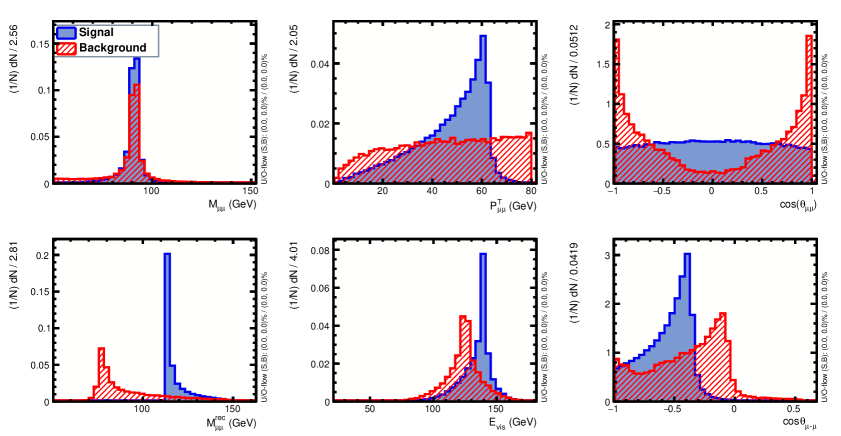
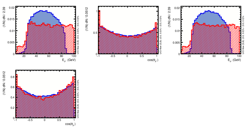
Figure 2: The input variables distributions for the lepton-related MVA. The variables are $M_{\mu^{+}\mu^{-}}$, $P^{T}_{\mu^{+}\mu^{-}}$, $\textrm{cos}\theta_{\mu^{+}\mu^{-}}$, $M^{\texttt{rec}}_{\mu^{+}\mu^{-}}$, $E_{\text{vis}}$, $\textrm{cos}\theta_{\mu^{+}-\mu^{-}}$, $E_{\mu^{+}}$, $\textrm{cos}\theta_{\mu^{+}}$, $E_{\mu^{-}}$, $\textrm{cos}\theta_{\mu^{-}}$, respectively.

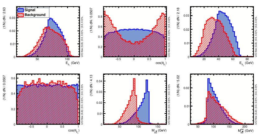
Figure 3: The input observable distributions for the jet-related MVA. The variables are $E_{b_{1}}$, $\textrm{cos}\theta_{b_{1}}$, $E_{b_{2}}$, $\textrm{cos}\theta_{b_{2}}$, $M_{b\bar{b}}$, $M^{\texttt{rec}}_{b\bar{b}}$, respectively.

,

The outputs of the two MVA are in Fig. 4, where the signal and backgrounds are well separated. After the kinematic cuts, the MVA cuts will be applied to further suppress the irreducible backgrounds.

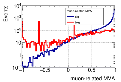
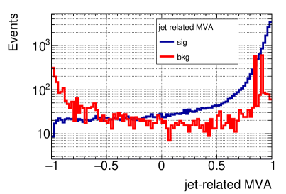
Figure 4: The lepton-related MVA output and the jet-related MVA output.

IV.3 Event selection and results

The background suppression is performed by maximizing signal significance, which is defined as $N_{sig}/\sqrt{(N_{sig}+N_{bkg})}$, where $N_{sig}$ and $N_{bkg}$ are the event numbers of the signal and background processes. The event numbers after cuts for the muon channel and electron channel are summarized in Tables 2 and 3, where the luminosity is 5600 $fb^{-1}$. The significance for the $Z\to\mu^{+}\mu^{-}$ channel is 114, while for the $Z\to e^{+}e^{-}$ channel is 109, which correspond to the uncertainties $\Delta\sigma(\mu^{+}\mu^{-}h)$ = 0.88% and $\Delta\sigma(e^{+}e^{-}h)$ =0.92%. Since the $Z\to b\bar{b}$ is well measured, and the Higgs decay is supposed to be the same as the SM Higgs boson, the above uncertainty is mainly caused by the anomalous $hZZ$ coupling. We cross-check our results with the CEPC experimental $\mu^{+}\mu^{-}h$ and $e^{+}e^{-}h$ measurements Bai et al. (2020). In the CEPC analysis, the Higgs bosons decaying to$b\bar{b}$, $c\bar{c}$ and $gg$ are combined together the significance after cuts are 96.4 for $\mu^{+}\mu^{-}h$ and 68.3 for $e^{+}e^{-}h$ after extrapolating the luminosity to 5600 $fb^{-1}$. Considering NLO effects and removing non-bjet backgrounds in their analysis, our results are consistent with theirs.

In order to include the full detector simulation effects, we apply the enhanced factor $k_{exp}$, which includes the detector effects, template fit and EFT fit effects. $k_{exp}$ is defined by $\frac{\Delta\sigma_{fast}}{\Delta\sigma_{full}}$, where $\Delta\sigma_{fast}$ is our result with the fast MC simulation and recoil mass method, and $\Delta\sigma_{full}$ is picked from the CEPC full simulation analysis with also the recoil mass method An et al. (2019). $k_{exp}$ is about 5.3, and the detailed calculation as well as the discussion can be found in Appendix B. After dividing $k_{exp}$, the uncertainty of $\Delta\sigma$ with explicit final state searching will reach 0.166% for $\Delta\sigma(\mu^{+}\mu^{-}h)$ and 0.173% for $\Delta\sigma(e^{+}e^{-}h)$. They are both smaller than the deviation induced by the IDM at 240 GeV in Table 1. If combining the different Higgs and $Z$ decay channels, the detective potential of the IDM model will be further improved. Thus, there is the opportunity to measure the deviation from the SM model by the loop effects in the IDM model at the CEPC.

Table 2: The cut table of $Z\to\mu^{+}\mu^{-}$ channel, when the luminosity is $\int Ldt=5600~{}fb^{-1}$.

$\int Ldt=5600~{}fb^{-1}$	$\mu^{+}\mu^{-}h_{\text{IDM}}$	2f	4f	Higgs	total backgrounds	efficiency	S/B	significance
Preselection	18547.4	7878	56776.1	140.4	64794.5	1	0.29	64.25
$M_{\mu^{+}\mu^{-}}\in[73,120]$ GeV	18000.6	6060	48647.6	131.8	54839.3	0.97	0.33	66.7
$P^{T}_{\mu^{+}\mu^{-}}\in[10,70]$ GeV	17679	3030	38429.5	129.5	41589	0.95	0.43	72.62
$E_{vis}\in[50,300]$ GeV	17679	3030	38429.5	124.1	41583.6	0.95	0.43	72.62
$M^{\texttt{rec}}_{\mu^{+}\mu^{-}}\in[110,155]$ GeV	17665.8	2424	6799.5	124	9347.5	0.95	1.89	107.48
$M_{b\bar{b}}\in[50,130]$ GeV	17514.9	2424	6306.7	114.8	8845.6	0.94	1.98	107.88
$M^{\texttt{rec}}_{b\bar{b}}\in[70,140]$ GeV	16244.1	1212	4549	77.5	5838.5	0.88	2.78	109.31
$\text{MVA}_{\mu}\in[-0.74,1]$	16240.7	1212	3793.9	77.5	5083.3	0.88	3.19	111.22
$\text{MVA}_{j}\in[-0.62,1]$	15829.8	1212	2166	68.1	3446.1	0.85	4.59	114.02

Table 3: The cut table of $Z\to e^{+}e^{-}$ channel, when the luminosity is $\int Ldt=5600~{}fb^{-1}$.

$\int Ldt=5600~{}fb^{-1}$	$e^{+}e^{-}h_{\text{IDM}}$	2f	4f	Higgs	total backgrounds	efficiency	S/B	significance
Preselection	18790.3	9090	88126.9	240.6	97457.5	1	0.19	55.11
$M_{e^{+}e^{-}}\in[73,120]$ GeV	17780.2	5454	62034.1	131	67619.1	0.95	0.26	60.84
$P^{T}_{e^{+}e^{-}}\in[10,70]$ GeV	17439.3	2424	51180.8	128.7	53733.5	0.93	0.32	65.37
$E_{vis}\in[50,300]$ GeV	17439.3	2424	51176.5	123.6	53724.1	0.93	0.32	65.37
$M^{\texttt{rec}}_{e^{+}e^{-}}\in[110,155]$ GeV	17411.8	606	8772.4	123.4	9501.8	0.93	1.83	106.13
$M_{b\bar{b}}\in[50,130]$ GeV	17183.7	606	8218.9	114.4	8939.3	0.91	1.92	106.32
$M^{\texttt{rec}}_{b\bar{b}}\in[70,140]$ GeV	15960.8	606	6151.0	76.6	6833.6	0.85	2.34	105.72
$\text{MVA}_{e}\in[-0.74,1]$	15959.1	606	5060.1	76.6	5742.7	0.85	2.78	108.33
$\text{MVA}_{j}\in[-0.62,1]$	15905	606	4604.6	75.4	5286	0.85	3.01	109.26

V Conclusion

We have performed the MC simulation of the lepton collider signals at electroweak one-loop level at future lepton colliders in synergy with the GW signals. The signals at future GW detectors and lepton colliders could make complementary exploration on the blind spots of this DM model. There is the opportunity to measure the deviation from the SM model by the loop effects in the IDM model at the future lepton colliders. In the future, if we observe the predicted GW signal at U-DECIGO, we would expect that the corresponding collider signals could be observed at the future lepton collider, and vice versa. Based on the study here, we will investigate more generic DM models with the blind spots, which might give more stronger collider and GW signals.

Appendix A Strong first-order phase transition

To discuss the phase transition dynamics in the IDM, we first write the Higgs doublet field $\Phi$ in terms of the background field $h$, namely,

$$\Phi=\begin{pmatrix}0\\ \frac{1}{\sqrt{2}}h\end{pmatrix}\,\,.$$ (30)

Further, the effective potential at the finite temperature can be obtained as

$$V_{\mathrm{eff}}(h,T)=V_{0}(h)+V_{\rm CW}(h)+V_{\rm ther}(h,T)+V_{\rm daisy}(h,T)\,\,.$$

$V_{0}(h)=\frac{\mu_{1}^{2}h^{2}}{2}+\frac{\lambda_{1}h^{4}}{4}$ is the tree-level potential. $V_{\rm CW}(h)$ is the Coleman-Weinberg potential at zero temperature. $V_{\rm ther}(h,T)$ is the thermal correction. $V_{\rm daisy}(h,T)$ represents the daisy resummation.The state-of-the-art calculations of the finite-temperature effective potential and its phase transition behavior are the recent two-loop investigations by Refs. Laine et al. (2017); Senaha (2019). Their results show that the one-loop effective potential in the high temperature expansion is rather reliable in the IDM Laine et al. (2017); Senaha (2019) and the corrections compared to one-loop results are small Laine et al. (2017); Senaha (2019). To clearly see the phase transition dynamics and simplify the following discussions on the phase transition GW signals, we only consider the one-loop effective potential including the daisy resummation. Since we only consider the IDM, only the Higgs doublet gets VEV. The phase transition along the Higgs field direction is favored in the benchmark points, which is well studied in previous literature Chowdhury et al. (2012); Borah and Cline (2012); Gil et al. (2012); Cline and Kainulainen (2013); AbdusSalam and Chowdhury (2014); Blinov et al. (2015); Cao et al. (2018); Huang and Yu (2018); Laine et al. (2017); Senaha (2019); Huang and Senaha (2019); Kainulainen et al. (2019).

The leading-order thermal corrections to the effective potential in the Landau gauge can be written as

$$V_{\rm ther}(h,T)=\frac{T^{4}}{2\pi^{2}}\left(\sum_{i=\mathrm{bosons}}n_{i}J_{B}\left[m^{2}_{i}(h)/T^{2}\right]+\sum_{i=\mathrm{fermions}}n_{i}J_{F}\left[m^{2}_{i}(h)/T^{2}\right]\right),$$ (31)

where the $J$ functions are defined as

$$J_{B}(x) =\int_{0}^{\infty}dt\;t^{2}\ln\left[1-\exp\left(-\sqrt{t^{2}+x}\right)\right]\,\,,$$ (32)

$$J_{F}(x) =\int_{0}^{\infty}dt\;t^{2}\ln\left[1+\exp\left(-\sqrt{t^{2}+x}\right)\right]\,\,.$$ (33)

Under high-temperature expansions, we have

$$T^{4}J_{B}\left[m^{2}/T^{2}\right] =-\frac{\pi^{4}T^{4}}{45}+\frac{\pi^{2}}{12}T^{2}m^{2}-\frac{\pi}{6}T\left(m^{2}\right)^{3/2}-\frac{1}{32}m^{4}\ln\frac{m^{2}}{a_{b}T^{2}}+\mathcal{O}\left(m^{2}/T^{2}\right)\,\,,$$ (34)

$$T^{4}J_{F}\left[m^{2}/T^{2}\right] =\frac{7\pi^{4}T^{4}}{360}-\frac{\pi^{2}}{24}T^{2}m^{2}-\frac{1}{32}m^{4}\ln\frac{m^{2}}{a_{f}T^{2}}+\mathcal{O}\left(m^{2}/T^{2}\right)\,\,,$$ (35)

where $a_{b}=16a_{f}=16\pi^{2}\exp(3/2-2\gamma_{E})$. In the above definition, the degree of freedom for the fermions is a negative integer to ensure a positive $T^{2}$ term. The positive $T^{2}$ terms for both bosons and fermions in the above expressions enable the symmetry restoration at high temperatures. The nonanalytic $m^{3}$ term in Eq. (34) can be responsible for the thermal barrier and the SFOPT between the high-temperature phase and the low-temperature phase.

The field-dependent masses of the gauge bosons and the top quark at zero temperature are given by

$$m_{W}^{2}(h) = \frac{g^{2}}{4}h^{2},\ m_{Z}^{2}(h)=\frac{g^{2}+g^{\prime 2}}{4}h^{2},m_{t}^{2}(h)=\frac{y_{t}^{2}}{2}h^{2},$$

where $y_{t}$ is the top Yukawa coupling, $g$ and $g^{\prime}$ are the gauge coupling of $SU(2)_{L}$ and $U(1)_{Y}$ gauge group, respectively. The field-dependent thermal scalar masses are

$$m_{h}^{2} =\lambda_{1}h^{2}\,\,,$$ (36)

$$m_{H}^{2} =\mu_{2}^{2}+\frac{1}{2}(\lambda_{3}+\lambda_{4}+\lambda_{5})h^{2}\,\,,$$ (37)

$$m_{A}^{2} =\mu_{2}^{2}+\frac{1}{2}(\lambda_{3}+\lambda_{4}-\lambda_{5})h^{2}\,\,,$$ (38)

$$m^{2}_{H^{+}} =\mu_{2}^{2}+\frac{1}{2}\lambda_{3}h^{2}\,\,.$$ (39)

In the above formulas, we have considered the contribution from daisy resummation in the Arnold-Espinosa scheme, which reads as

$$V_{daisy} \supset -\frac{T}{12\pi}\sum_{i={\rm b}}n_{b}\left(\left[m_{i}^{2}(h,T)\right]^{3/2}-\left[m_{i}^{2}(h)\right]^{3/2}\right)\,\,.$$

Here, the thermal field-dependent masses $m_{i}^{2}(h,T)\equiv m_{i}^{2}(h)+\Pi_{i}(h,T)$, where $\Pi_{i}(h,T)$ is the bosonic field $i$’s self-energy in the IR limit.

All the scalar particles can get a thermal mass by replacing

$$\mu_{2}^{2}\to\mu_{2}^{2}+c_{2}T^{2}$$ (40)

$$\mu_{1}^{2}\to\mu_{1}^{2}+c_{1}T^{2}$$ (41)

with the thermal correction coefficients

$$c_{1}=\frac{3\lambda_{1}+2\lambda_{3}+\lambda_{4}}{12}+\frac{3g^{2}+g^{{}^{\prime}2}}{16}+\frac{y_{t}^{2}}{4}\,\,,$$ (42)

$$c_{2}=\frac{3\lambda_{2}+2\lambda_{3}+\lambda_{4}}{12}+\frac{3g^{2}+g^{{}^{\prime}2}}{16}\,\,.$$ (43)

There is no thermal mass corrections for the fermions and the transverse component of the gauge bosons at leading order. Only the longitudinal component of the gauge boson has the thermal mass corrections, namely,

$$\Pi_{W}(T)=2g^{2}T^{2}\,\,,$$ (44)

$$\Pi_{B}(T)=2g^{{}^{\prime}2}T^{2}\,\,.$$ (45)

To calculate the effective potential in IDM, the degrees of freedom for each particles running in the loop are shown below:

$$n_{W^{\pm}}=4,\ n_{Z}=2,\ n_{\pi}=3\,\,,$$

$$\ n_{h}=n_{H}=n_{H^{+}}=n_{H^{+}}=1,\ n_{t}=-12\,\,.$$

Appendix B The analysis with the model-independent method

We perform the model-independent measurement for the $hZZ$ coupling in Table 4. The analysis algorithms are the same as the CEPC/ILC experimental analysis with the recoil mass technique. In the whole analysis, only $Z$ decay products, i.e., $\mu^{+}\mu^{-}$, are used to constitute the kinematics as $M_{\mu^{+}\mu^{-}}$, $P^{T}_{\mu^{+}\mu^{-}}$, no information from the h decay products are involved. Thus, the measurement for $hZZ$ coupling would not depend on model-specific assumptions on the properties of the Higgs boson. However, this method will also decrease the significance when searching new phenomena. For example, in the following analysis, with the same datasets, the maximum significance is about 38, which is obviously smaller than the results with explicit Higgs decay final states in Table 2.

The corresponding uncertainty with model-independent measurement is $\Delta\sigma\sim 2.6\%$. It is similar to the result in the CEPC report Dong et al. (2018), which only applied the kinematic cuts. In our paper, the parton-level event generation and hadronizations are completely the same with the generation in CEPC, including the luminosity, the simulation event number and weight, and so on. The difference only comes from the detector simulation and following signal analysis. In CEPC collaboration’s analysis with full detector simulation events, after the normal kinematic cuts, they applied the template fit and the parameter fit to combine the CEPC and HL-LHC data An et al. (2019), then $\Delta\sigma$ will further reach the report value 0.5%. In this work, we use the CEPC default Delphes Card for detector simulation in Delphes and we only add normal kinematic cuts for signal analysis, without template fit and the parameter fit. As a result, comparing our results and the CEPC results, the ratio of the significance would reflect the differences from the detector simulation and the following analysis procedures. Thus, in this note, we define the enhanced factor $k_{exp}$ to include the full-simulation effects, template fit cut effect, EFT fitting with LHC data and all other related effects. $k_{exp}$ of the CEPC collaboration reported $\Delta\sigma$ to our simulated value is about 5.3. We also assume $k_{exp}$ is the same for the $Z\to e^{+}e^{-}$ channel and the $Z\to\mu^{+}\mu^{-}$ channel. We will use this enhanced factor to estimate the measurement uncertainties of $hZZ$ with the explicit Higgs decay final states at the CEPC in Sec. IV.3.

Table 4: The cut table of $Z\to\mu^{+}\mu^{-}$ channel with a model-independent measurements, when the luminosity is $\int Ldt=5600~{}fb^{-1}$.

$\int Ldt=5600~{}fb^{-1}$	$\mu^{+}\mu^{-}h_{\text{IDM}}$	2f	4f	Higgs	total	efficiency	S/B	significance
Preselection	19841	1.89$\times 10^{6}$	717156	12195.9	2.62$\times 10^{6}$	1	0.008	12.21
$M_{\mu^{+}\mu^{-}}\in[73,120]$ GeV	19238.5	1.51$\times 10^{6}$	486730	11764.5	2.01$\times 10^{6}$	0.97	0.01	13.52
$P^{T}_{\mu^{+}\mu^{-}}\in[10,70]$ GeV	18890.9	481428	402934	11552.8	895915	0.95	0.02	19.75
$E_{vis}\in[50,300]$ GeV	18890.9	466789	308576	11187.9	786553	0.95	0.02	21.05
$\text{MVA}_{\mu}\in[-0.74,1]$	18877.7	158664	64050.7	10582.6	233297	0.95	0.08	37.59
$M^{\texttt{rec}}_{\mu^{+}\mu^{-}}\in[110,155]$ GeV	18864.4	154942	62779	10575.7	228297	0.95	0.08	37.94

References

- Bertone and Hooper (2018) G. Bertone and D. Hooper, Rev. Mod. Phys. 90, 045002 (2018), arXiv:1605.04909 [astro-ph.CO] .
- Barbieri et al. (2006) R. Barbieri, L. J. Hall, and V. S. Rychkov, Phys. Rev. D 74, 015007 (2006), arXiv:hep-ph/0603188 .
- Lopez Honorez and Yaguna (2010) L. Lopez Honorez and C. E. Yaguna, JHEP 09, 046 (2010), arXiv:1003.3125 [hep-ph] .
- Dong et al. (2018) M. Dong et al. (CEPC Study Group), (2018), arXiv:1811.10545 [hep-ex] .
- An et al. (2019) F. An et al., Chin. Phys. C 43, 043002 (2019), arXiv:1810.09037 [hep-ex] .
- Abada et al. (2019) A. Abada et al. (FCC), Eur. Phys. J. ST 228, 261 (2019).
- Fujii et al. (2017) K. Fujii et al., (2017), arXiv:1710.07621 [hep-ex] .
- Chowdhury et al. (2012) T. A. Chowdhury, M. Nemevsek, G. Senjanovic, and Y. Zhang, JCAP 02, 029 (2012), arXiv:1110.5334 [hep-ph] .
- Aprile et al. (2018) E. Aprile et al. (XENON), Phys. Rev. Lett. 121, 111302 (2018), arXiv:1805.12562 [astro-ph.CO] .
- Barducci et al. (2018) D. Barducci, G. Belanger, J. Bernon, F. Boudjema, J. Da Silva, S. Kraml, U. Laa, and A. Pukhov, Comput. Phys. Commun. 222, 327 (2018), arXiv:1606.03834 [hep-ph] .
- Aghanim et al. (2018) N. Aghanim et al. (Planck), (2018), arXiv:1807.06209 [astro-ph.CO] .
- Borah and Cline (2012) D. Borah and J. M. Cline, Phys. Rev. D 86, 055001 (2012), arXiv:1204.4722 [hep-ph] .
- Gil et al. (2012) G. Gil, P. Chankowski, and M. Krawczyk, Phys. Lett. B 717, 396 (2012), arXiv:1207.0084 [hep-ph] .
- Cline and Kainulainen (2013) J. M. Cline and K. Kainulainen, Phys. Rev. D 87, 071701 (2013), arXiv:1302.2614 [hep-ph] .
- AbdusSalam and Chowdhury (2014) S. S. AbdusSalam and T. A. Chowdhury, JCAP 05, 026 (2014), arXiv:1310.8152 [hep-ph] .
- Blinov et al. (2015) N. Blinov, S. Profumo, and T. Stefaniak, JCAP 07, 028 (2015), arXiv:1504.05949 [hep-ph] .
- Cao et al. (2018) Q.-H. Cao, F. P. Huang, K.-P. Xie, and X. Zhang, Chin. Phys. C 42, 023103 (2018), arXiv:1708.04737 [hep-ph] .
- Huang and Yu (2018) F. P. Huang and J.-H. Yu, Phys. Rev. D 98, 095022 (2018), arXiv:1704.04201 [hep-ph] .
- Laine et al. (2017) M. Laine, M. Meyer, and G. Nardini, Nucl. Phys. B 920, 565 (2017), arXiv:1702.07479 [hep-ph] .
- Senaha (2019) E. Senaha, Phys. Rev. D 100, 055034 (2019), arXiv:1811.00336 [hep-ph] .
- Huang and Senaha (2019) F. P. Huang and E. Senaha, Phys. Rev. D 100, 035014 (2019), arXiv:1905.10283 [hep-ph] .
- Kainulainen et al. (2019) K. Kainulainen, V. Keus, L. Niemi, K. Rummukainen, T. V. Tenkanen, and V. Vaskonen, JHEP 06, 075 (2019), arXiv:1904.01329 [hep-ph] .
- Belyaev et al. (2018) A. Belyaev, G. Cacciapaglia, I. P. Ivanov, F. Rojas-Abatte, and M. Thomas, Phys. Rev. D 97, 035011 (2018), arXiv:1612.00511 [hep-ph] .
- Wainwright (2012) C. L. Wainwright, Comput. Phys. Commun. 183, 2006 (2012), arXiv:1109.4189 [hep-ph] .
- Branco et al. (2012) G. C. Branco, P. M. Ferreira, L. Lavoura, M. N. Rebelo, M. Sher, and J. P. Silva, Phys. Rept. 516, 1 (2012), arXiv:1106.0034 [hep-ph] .
- Hindmarsh et al. (2014) M. Hindmarsh, S. J. Huber, K. Rummukainen, and D. J. Weir, Phys. Rev. Lett. 112, 041301 (2014), arXiv:1304.2433 [hep-ph] .
- Hindmarsh et al. (2015) M. Hindmarsh, S. J. Huber, K. Rummukainen, and D. J. Weir, Phys. Rev. D 92, 123009 (2015), arXiv:1504.03291 [astro-ph.CO] .
- Hindmarsh et al. (2017) M. Hindmarsh, S. J. Huber, K. Rummukainen, and D. J. Weir, Phys. Rev. D 96, 103520 (2017), [Erratum: Phys.Rev.D 101, 089902 (2020)], arXiv:1704.05871 [astro-ph.CO] .
- Wang et al. (2020a) X. Wang, F. P. Huang, and X. Zhang, JCAP 05, 045 (2020a), arXiv:2003.08892 [hep-ph] .
- Turner et al. (1992) M. S. Turner, E. J. Weinberg, and L. M. Widrow, Phys. Rev. D 46, 2384 (1992).
- Caprini et al. (2020) C. Caprini et al., JCAP 03, 024 (2020), arXiv:1910.13125 [astro-ph.CO] .
- Ellis et al. (2019) J. Ellis, M. Lewicki, J. M. No, and V. Vaskonen, JCAP 06, 024 (2019), arXiv:1903.09642 [hep-ph] .
- Kosowsky et al. (2002) A. Kosowsky, A. Mack, and T. Kahniashvili, Phys. Rev. D 66, 024030 (2002), arXiv:astro-ph/0111483 .
- Gogoberidze et al. (2007) G. Gogoberidze, T. Kahniashvili, and A. Kosowsky, Phys. Rev. D 76, 083002 (2007), arXiv:0705.1733 [astro-ph] .
- Niksa et al. (2018) P. Niksa, M. Schlederer, and G. Sigl, Class. Quant. Grav. 35, 144001 (2018), arXiv:1803.02271 [astro-ph.CO] .
- Caprini et al. (2009) C. Caprini, R. Durrer, and G. Servant, JCAP 12, 024 (2009), arXiv:0909.0622 [astro-ph.CO] .
- Caprini et al. (2016) C. Caprini et al., JCAP 04, 001 (2016), arXiv:1512.06239 [astro-ph.CO] .
- Moore and Prokopec (1995) G. D. Moore and T. Prokopec, Phys. Rev. D 52, 7182 (1995), arXiv:hep-ph/9506475 .
- Wang et al. (2020b) X. Wang, F. P. Huang, and X. Zhang, (2020b), arXiv:2011.12903 [hep-ph] .
- Giese et al. (2021) F. Giese, T. Konstandin, K. Schmitz, and J. Van De Vis, JCAP 01, 072 (2021), arXiv:2010.09744 [astro-ph.CO] .
- Wang et al. (2021) X. Wang, F. P. Huang, and X. Zhang, Phys. Rev. D 103, 103520 (2021), arXiv:2010.13770 [astro-ph.CO] .
- Kudoh et al. (2006) H. Kudoh, A. Taruya, T. Hiramatsu, and Y. Himemoto, Phys. Rev. D 73, 064006 (2006), arXiv:gr-qc/0511145 .
- Corbin and Cornish (2006) V. Corbin and N. J. Cornish, Class. Quant. Grav. 23, 2435 (2006), arXiv:gr-qc/0512039 .
- Amaro-Seoane et al. (2017) P. Amaro-Seoane et al. (LISA), (2017), arXiv:1702.00786 [astro-ph.IM] .
- (45) https://www.cosmos.esa.int/web/lisa/lisa-documents.
- Luo et al. (2016) J. Luo et al. (TianQin), Class. Quant. Grav. 33, 035010 (2016), arXiv:1512.02076 [astro-ph.IM] .
- Hu et al. (2018) X.-C. Hu, X.-H. Li, Y. Wang, W.-F. Feng, M.-Y. Zhou, Y.-M. Hu, S.-C. Hu, J.-W. Mei, and C.-G. Shao, Class. Quant. Grav. 35, 095008 (2018), arXiv:1803.03368 [gr-qc] .
- Mei et al. (2020) J. Mei et al. (TianQin), (2020), 10.1093/ptep/ptaa114, arXiv:2008.10332 [gr-qc] .
- Hu and Wu (2017) W.-R. Hu and Y.-L. Wu, Natl. Sci. Rev. 4, 685 (2017).
- Ruan et al. (2020) W.-H. Ruan, Z.-K. Guo, R.-G. Cai, and Y.-Z. Zhang, Int. J. Mod. Phys. A 35, 2050075 (2020), arXiv:1807.09495 [gr-qc] .
- Seto et al. (2001) N. Seto, S. Kawamura, and T. Nakamura, Phys. Rev. Lett. 87, 221103 (2001), arXiv:astro-ph/0108011 .
- Kawamura et al. (2011) S. Kawamura et al., Class. Quant. Grav. 28, 094011 (2011).
- Guo et al. (2021) H.-K. Guo, K. Sinha, D. Vagie, and G. White, JCAP 01, 001 (2021), arXiv:2007.08537 [hep-ph] .
- Croon et al. (2020) D. Croon, O. Gould, P. Schicho, T. V. I. Tenkanen, and G. White, (2020), arXiv:2009.10080 [hep-ph] .
- Kilian et al. (2011) W. Kilian, T. Ohl, and J. Reuter, Eur. Phys. J. C 71, 1742 (2011), arXiv:0708.4233 [hep-ph] .
- De Blas et al. (2019) J. De Blas, G. Durieux, C. Grojean, J. Gu, and A. Paul, JHEP 12, 117 (2019), arXiv:1907.04311 [hep-ph] .
- Bambade et al. (2019) P. Bambade et al., (2019), arXiv:1903.01629 [hep-ex] .
- Arhrib et al. (2015) A. Arhrib, R. Benbrik, J. El Falaki, and A. Jueid, JHEP 12, 007 (2015), arXiv:1507.03630 [hep-ph] .
- Kanemura et al. (2016) S. Kanemura, M. Kikuchi, and K. Sakurai, Phys. Rev. D 94, 115011 (2016), arXiv:1605.08520 [hep-ph] .
- Barklow et al. (2018) T. Barklow, K. Fujii, S. Jung, M. E. Peskin, and J. Tian, Phys. Rev. D 97, 053004 (2018), arXiv:1708.09079 [hep-ph] .
- Mo et al. (2016) X. Mo, G. Li, M.-Q. Ruan, and X.-C. Lou, Chin. Phys. C 40, 033001 (2016), arXiv:1505.01008 [hep-ex] .
- Sjostrand et al. (2006) T. Sjostrand, S. Mrenna, and P. Z. Skands, JHEP 05, 026 (2006), arXiv:hep-ph/0603175 .
- de Favereau et al. (2014) J. de Favereau, C. Delaere, P. Demin, A. Giammanco, V. Lemaître, A. Mertens, and M. Selvaggi (DELPHES 3), JHEP 02, 057 (2014), arXiv:1307.6346 [hep-ex] .
- Quinlan (1987) J. Quinlan, International Journal of Man-Machine Studies 27, 221 (1987).
- Brun and Rademakers (1997) R. Brun and F. Rademakers, Nuclear Instruments and Methods in Physics Research Section A: Accelerators, Spectrometers, Detectors and Associated Equipment 389, 81 (1997), new Computing Techniques in Physics Research V.
- Bai et al. (2020) Y. Bai, C. Chen, Y. Fang, G. Li, M. Ruan, J.-Y. Shi, B. Wang, P.-Y. Kong, B.-Y. Lan, and Z.-F. Liu, Chin. Phys. C 44, 013001 (2020), arXiv:1905.12903 [hep-ex] .