GAEA: Graph Augmentation for Equitable Access via Reinforcement Learning

Abstract

Disparate access to resources by different subpopulations is a prevalent issue in societal and sociotechnical networks. For example, urban infrastructure networks may enable certain racial groups to more easily access resources such as high-quality schools, grocery stores, and polling places. Similarly, social networks within universities and organizations may enable certain groups to more easily access people with valuable information or influence. Here we introduce a new class of problems, Graph Augmentation for Equitable Access (GAEA), to enhance equity in networked systems by editing graph edges under budget constraints. We prove such problems are NP-hard, and cannot be approximated within a factor of $(1-\tfrac{1}{3e})$. We develop a principled, sample- and time- efficient Markov Reward Process (MRP)-based mechanism design framework for GAEA. Our algorithm outperforms baselines on a diverse set of synthetic graphs. We further demonstrate the method on real-world networks, by merging public census, school, and transportation datasets for the city of Chicago and applying our algorithm to find human-interpretable edits to the bus network that enhance equitable access to high-quality schools across racial groups. Further experiments on Facebook networks of universities yield sets of new social connections that would increase equitable access to certain attributed nodes across gender groups.

Introduction

Designing systems and infrastructures to enable equitable access to resources has been a longstanding problem in economics, planning, and public policy. A classical setting where equity is a strong design criterion is facility location for public goods such as schools, grocery stores, and voting booths (Mumphrey, Seley, and Wolpert 1971; McAllister 1976; Mandell 1991). Since individual-level fairness is often impossible for these spatially-structured problems, the focus has been on group-level fairness; several metrics have been proposed and optimized (Marsh and Schilling 1994), including simultaneous optimization of several metrics (Gupta et al. 2020). In this paper, we take up the same challenge of equitable access to resources, but for network-structured rather than spatially-structured problems. We specifically consider editing the edges of graphs under budget constraints to improve equity in group-level access, under a diffusion model of mobility dynamics. We use the demographic parity metric (Verma and Rubin 2018). In economics, a common measure of (in)equity called the Gini index is often used to characterize the statistical dispersion in income or wealth, but also access to resources at individual or group levels (Cole et al. 2018; Malakar, Mishra, and Patwardhan 2018), which we also measure.

Facility location problems (not considering equity) have been well-studied in network settings for applications in epidemiology (Nowzari, Preciado, and Pappas 2016; Zhang et al. 2019), surveillance (Leskovec et al. 2007), and influence maximization (Li et al. 2018; Kempe, Kleinberg, and Tardos 2003). These involve changing node properties of a graph; contrarily we edit the edges of graphs. Formally we prove our graph editing problem—Graph Augmentation for Equitable Access (GAEA)—is a generalization of facility location and that it is NP-hard.

In urban transportation networks, different racial, ethnic, or socioeconomic groups may have varying access to high-quality schools, libraries, grocery stores, and voting booths, which in turn lead to disparate health and educational outcomes, and political power. Interventions to enhance equity in transportation networks may include increasing public transit for the most effective paths to resources such as high-quality schools. From an implementation perspective, changing bus routes may be easier than relocating schools. We do not consider strategic aspects of congestion in transportation networks (Youn, Gastner, and Jeong 2008).

In social networks within organizations like schools, people in different racial or gender groups may have varying access to specific people that hold valuable information or have significant influence, whom we cast as network resources. This in turn may lead to disparate outcomes in social life. Interventions to enhance equity include encouraging friendship between specific individuals in the social network. This can be done, e.g. in university settings by offering free meals for two specific people to meet: what we call buddy lunches.

Since AI models are embedded in numerous consequential sociotechnical systems, ensuring equity in their operation has emerged as a fundamental challenge (Dwork and Ilvento 2018; Mehrabi et al. 2019). Of more relevance to us, however, AI techniques are being used to design equitable public policies e.g. for taxation (Zheng et al. 2020). Here we use AI methods for system/infrastructure redesign to increase equitable access to resources for settings such as transportation networks (Hay and Trinder 1991; Bowerman, Hall, and Calamai 1995) and social networks (Abebe et al. 2019; Fish et al. 2019). In particular, we develop a Markov Reward Process (MRP) framework and a principled, sample- and time-efficient reinforcement learning technique for the GAEA optimization. Our approach produces interpretable, localized graph edits and outperforms deterministic baselines on both synthetic and real-world networks.

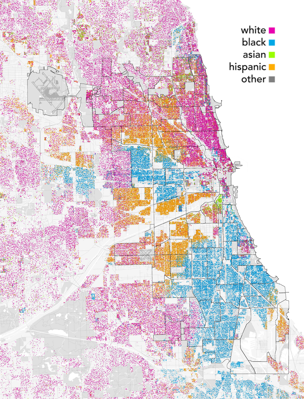
(a) Chicago demographics by race/ethnicity

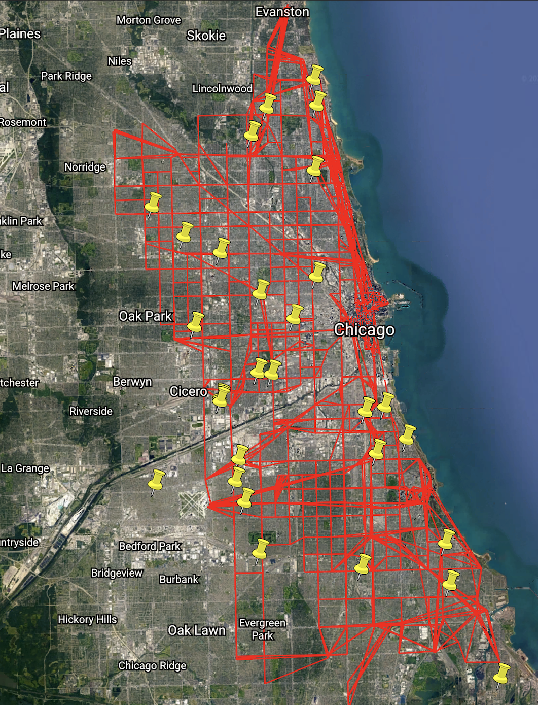
(b) Chicago transit network and school locations

Figure 1: Chicago demographics and infrastructure, (a) shows demographics, demonstrating highly segregated areas of the city by race and ethnicity; (b) shows a transit network (red) we collected for this work, induced from Chicago Transit Authority bus routes. We also show (yellow) the location of schools within our dataset from the Chicago Public Schools.

We demonstrate the effectiveness of our approach on real-world transportation network data from the City of Chicago. Chicago is the most spatially segregated city in the United States via 2010 census data (Logan 2014). At the same time, prior work shows this segregation yields significant disparity in education (Groeger, Waldman, and Eads 2018) and health (Orsi, Margellos-Anast, and Whitman 2010) outcomes by race and ethnicity, particularly among White, Black, and Hispanic communities. In the Chicago Public School District $299$—constituting the entire city of Chicago—White students are the equivalent of $3$ academic years ahead of Black students, and $2.3$ years ahead of Hispanic students. Our technique yields an edited graph which reduces disparity in physical access to high-quality schools.

We also present a similar analysis for gender in university social networks using the node-attributed Facebook100 network data (Traud, Mucha, and Porter 2012).

Contributions

Our main contributions are as follows.

• The novel Graph Augmentation for Equitable Access (GAEA) problem, which generalizes facility location, and which we prove is NP-hard.

• Markov Reward Process framework to address this difficult optimization problem, yielding principled, sample- and time-efficient mechanism design based on reinforcement learning.

• Demonstration of efficacy in both synthetic and real-world networks (transportation and social), showing performance improvement over deterministic baselines.

Related Work

Equity in AI

Recent work on fairness in machine learning has expanded very rapidly. Mehrabi et al. (2019) outline $23$ definitions of bias introduced from underlying AI models, $6$ definitions of discrimination (i.e. the prejudicial and disparate impacts of bias), and $10$ definitions of fairness which mitigate these impacts. There is a similar zoo of definitions for equity in facility location (Marsh and Schilling 1994). We focus here on demographic parity.

This is the first work measuring and mitigating inequity within an arbitrarily-structured graph environment.

Graph Diffusion, Augmentation, and Reinforcement Learning

Our formulation of equitable access lies within a larger body of work on diffusion in graphs. Prior work has examined event detection time in sensor networks (Leskovec et al. 2007), or influence maximization in social networks (Li et al. 2018; Kempe, Kleinberg, and Tardos 2003). The problem can also be viewed as maximization of graph connectivity, maximization of spectral radius, or maximization of closeness centrality of reward nodes (Crescenzi et al. 2016).

Graph augmentation is a class of combinatorial graph problems to identify the minimum-sized set of edges to add to a graph to satisfy some connectivity property, such as $k$-connectivity or strong connectedness (Hsu and Ramachandran 1993): our objective is not such a straightforward combinatorial property.

Prior work in graph reinforcement learning primarily focuses on coordinating agents with respect to local structure for cooperative and/or competitive tasks (Carion et al. 2019). Our work differs in that we learn a system design policy rather than coordination among active agents.

Problem Definition

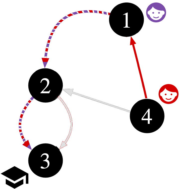
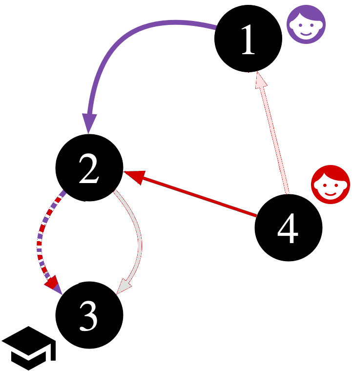
Figure 2: A before and after equitable graph augmentation of a toy schematic showing school access between two disparate populations distributed spatially different from each other. Individuals from the group traverse along the edges of their respective color.

Toy Example

Figure 2 shows a toy example of our problem. Assume we have a fixed topology where new edges can form, shown in the figure as gray arrows. We have two distinct population of purple and red individuals distributed differently over the nodes of the graph. Based on the graph edges, each group has different levels of access to the same resources, in this case access to schools. The individuals of purple population can access the school at node 3 in two hops 1-2-3, whereas individuals of red population have to traverse one extra hop i.e. 4-1-2-3 to access the same resource.

Suppose we have a budget to edit one edge, forming the edge 4-2 will match the red and purple population’s access to school. If we have one more edge in the budget, augmenting the additional edge 2-3 will improve access for both populations equitably. This sequence of edge augmentations that improve resource access for the overall population and at the same time maintains equity among subpopulations is what this work strives to achieve. We restrict edge formation to a predefined topology, since arbitrary edge formations are not feasible in many real sociotechnical graphs, e.g. in spatial graphs, an edge between two nodes that are arbitrarily far apart cannot be formed.

Preliminaries

Let graph $\mathbb{G}=(V,E)$ have vertex set $V=\{v_{1},\dots,v_{n}\}$ of size $n$ and edge set $E=\{e_{i,j}\}$ of size $m$. Edges are unweighted and directed. Let $G$ be a set of groups such as racial or gender groups. Let reward nodes be a subset of nodes $R\subseteq V$.

We consider a particle $p_{g}\in V$ of group $g\in G$ as an instance of starting node positions sampled from a group-specific distribution $\mu_{0}(g)$. Letting $d(p_{g},r)$ be the shortest path for particle $p_{g}$ along edges $E$ of $\mathbb{G}$ to reach a reward node in $R$, we define a utility function for each group as:

$${u_{g}(p_{g};E)={\operatorname*{\mathbb{E}}}_{{p_{g}\sim\mu(g)}}\tfrac{1}{d(p_{g},r)}\mbox{.}}$$ (1)

The utility function is parameterized by the edge set $E$. For simplicity, we refer to $u_{g}(p_{g};E)$ as just $u_{g}$ and define the utility of the entire group $g$ as:

$${U_{g}={\operatorname*{\mathbb{E}}}_{{{p_{g}\sim\mu(g)}}}[u_{g}]\mbox{.}}$$ (2)

We define $\overline{U}_{G}=\sum_{c\in G}U_{g}/|G|$ as mean utility of all groups and inequity as deviation of group utilities from the mean. i.e $\sum_{g\in G}{|U_{g}-\overline{U}_{G}|}$. To minimize inequity is to minimize this difference. Finally, let a graph augmentation function for a budget $B$ be defined as:

$${e:\mathbb{G},B\rightarrow\mathbb{G}^{\prime}}$$ (3)

where $\mathbb{G}^{\prime}=(V,E\cup E^{u})$, $E^{u}$ is the edge augmentation to the graph $\mathbb{G}$ constrained by budget $B$, under Hamming distance $\mathcal{D}(\mathbb{G}-\mathbb{G}^{\prime})<B$.

Methods

Now let us formalize our problem definition.

Find: $\mathbb{G}^{\prime}=e(\mathbb{G},B)$

Where: $\mathbb{G}^{\prime}=\operatorname*{argmax}\limits_{\begin{subarray}{c}s.t.\sum_{g\in G}{|U_{g}-\overline{U}_{G}|}=0\\ {{\mathcal{D}}(\mathbb{G}-\mathbb{G}^{\prime})<B}\end{subarray}}{\operatorname*{\mathbb{E}}}_{{g\in G}}[U_{g}]$

Problem 1 Graph Augmentation for Equitable Access

Greedy Baseline

For prior baseline, to the best of our knowledge we are not aware of earlier works that does budgeted discrete equitable graph augmentation that maximize utility of disparate groups. That said, we observe that without equitable access across groups, optimizing for maximum utility, $U_{g}$ alone reduces the problem to maximizing centrality of the reward nodes $r\in R$. Hence we extend the greedy improvement for any monotone submodular $U_{g}$ proposed by (Crescenzi et al. 2016) to the equitable group access setting, which we call Greedy Equitable Centrality Improvement (GECI) baseline. For a given edge set $E$, we define neighborhood $N_{g}(E)$ as all nodes $u\in V$ and $u\not\in E$ that are in the shortest path to reward node $r$ less than $T$ steps for candidate from group $g$. With budget $B$, the GECI method is defined in Method 2.

Input: A directed graph $\mathbb{G}=(V,E)$, neighborhood function $N_{g}$, and budget $B$

$E^{u}:=\emptyset$

for  $b=1,2,\dots,B$ do

       $E^{e}:=E\cup E^{u}$ $g_{\min}:=\operatorname*{argmin}{\{U_{g}(E^{e})|g\in G)\}}$

       for  $u\in V|u\in N_{g_{min}}(E^{e})$ do

             for $v\in V|v\in E^{e}$ do

                   Compute $U_{g_{\min}}(E^{e}\cup\{(u,v)\})$

      $u_{\max},v_{\max}:=\operatorname*{argmax}{\{U_{g_{\min}}(E^{e}\cup\{(u,v)\})\}}$

       $E^{u}:=E^{u}\cup\{(u_{\max},v_{\max})\}$

return $E^{u}$

Method 2 Greedy equitable centrality improvement

For every augmentation of edge $E^{u}$, we pick the group $g_{\min}$ that is most disadvantageous or in other words the group with least group utility $U_{g}$. We then pick a pair of nodes $(u_{\max},v_{\max})$ to form an edge augmentation, such that nodes $v_{\max}$ and $u_{\max}$ are in $E$ and in the neighborhood $N_{g_{min}}$ respectively and result in maximum change in most disadvantageous group’s utility $U_{g_{\min}}$, for the candidate group $g_{\min}$, We update the edge augmentation set $E^{u}:=E^{u}\cup\{(u_{\max},v_{\max})\}$. The graph augmentation step is repeated until the budget $B$ is exhausted.

Optimization Formulation

Let us consider the GAEA problem from an optimization perspective. Let $U_{g}$ be the expected utility of a group. Then Pareto optimality of utilities of all groups can be framed as:

$${J=\max\limits_{\begin{subarray}{c}s.t.\sum_{g\in G}{|U_{g}-\overline{U}_{G}|}=0\\ \sum_{g\in G}{\left\lVert E^{u}\right\rVert_{0}<B}\end{subarray}}{\operatorname*{\mathbb{E}}}_{{g\in G}}[U_{g}]}\mbox{.}$$ (4)

The first constraint in (4) is the equity constraint while the second is the budget constraint. The constraints are non-differentiable, especially the number of discrete edges to edit, and cannot be solved directly using typical algorithms. Hence we develop our learning approach.

Equitable Mechanism Design in MRP

We frame the graph, $\mathbb{G}=(V,E)$, and dynamic process of reaching reward nodes by particles of different group, $g\in G$, as mechanism design of a finite-horizon Markov Reward Process (MRP). The MRP consists of a finite set of states, $S$; dynamics of the system defined by a set of Markov state transition probability $P$; a reward function, $R\in\mathbb{R}^{|S|}$; and a horizon defined by the maximum time step $T$ reachable in a random walk. Here states $S$ corresponds to vertices $V$ of the graph $\mathbb{G}$, and the transition dynamics are parameterized by $P=D^{-1}E$, with diagonal matrix $D(i,i)=\sum_{j}E_{(i,j)}$. Unlike Markov Decision Processes (MDP), MRP does not optimize for a policy, instead optimizing for dynamics that maximize the state value function.

The state value function of the MRP for a particle, $p_{g}$ of group $g$, spawned at state $s_{0}$ is given by:

$${v_{g}(s_{0})=\sum_{t=0}^{T-1}\gamma^{t}RP^{t}s_{0}\mbox{,}}$$ (5)

where $\gamma\in[0,1]$ is the discount factor. This $\gamma$ encourages the learning system to choose shorter paths reachable under the horizon $T$. The expected value function for the group, $g$, is:

$${V^{g}={\operatorname*{\mathbb{E}}}_{{s_{0}\sim\mu(g)}}[v^{g}(s_{0})]\mbox{.}}$$ (6)

We parameterize the transition probability as $P=D^{-1}E^{e}$, where $E^{e}=E+A\odot E^{u}$ and diagonal matrix $D$ satisfies $D(i,i)=\sum_{j}E^{e}(i,j)$.

Here $E\in\{0,1\}^{|S|\times|S|}$ is the edge-adjacency matrix of the unedited original graph $\mathbb{G}$. Further, $A\in\{0,1\}^{|S|\times|S|}$ is a mask adjacency matrix corresponding to given topology, used to restrict the candidate edges for edit. This restriction is useful for spatial graphs where very distant nodes cannot realistically form an edge. The set $E^{u}\in\{0,1\}^{|S|\times|S|}$ is the learned discrete choice of edges that are augmented. To make discrete edge augmentation $E^{u}$ differentiable, we perform continuous relaxation, with reparameterization trick using Gumbel sigmoid (Jang, Gu, and Poole 2016), defined by

$${E^{u}{(i,j)}=\frac{1}{(1+\exp(-(\phi(\vec{0})+g_{i})/\tau)},\forall i,j\in S}$$ (7)

where, $g_{i}=-\log(-\log(\mathbb{U}))$ and $\mathbb{U}$ are the Gumbel noise and uniform random noise respectively. Over the period of training, the temperature $\tau$ is attenuated. As $\tau\to 0$, $E_{g}^{u}$ becomes discrete. Hence we gradually attenuate $\tau\leftarrow\tau*\nu$ at every epoch with a decay factor $\nu$ . Note that the function $\phi(\cdot)$ in (7) takes the zero vector as input, which effectively forces the function to learn only the bias term and makes the choice of edits independent of the input state. The problem objective under MRP framing is:

$${E^{u}=\operatorname*{argmax}\limits_{\begin{subarray}{c}s.t.\sum_{g\in G}|V_{g}-\overline{V}_{G}|=0\\ \sum_{g\in G}\left\lVert E^{u}\right\rVert_{0}<B\end{subarray}}\sum_{g\in G}V_{g}\mbox{.}}$$ (8)

Here $\overline{V}_{G}={\sum_{g\in G}V_{g}}/{|G|}$. We recast the constrained optimization as unconstrained optimization using augmented Lagrangian (Nocedal and Wright 2006), as:

$$\begin{multlined}{J=-\min_{E^{u}}\sum_{g\in G}{V^{g}}\\ -\mu_{1}(\sum_{g\in G}{V_{g}-\overline{V_{G}})}^{2}-\mu_{2}(\min(0,\sum_{g\in G}{\left\lVert E^{u}\right\rVert_{0}-B))}^{2}\\ -\lambda_{1}(\sum_{g\in G}{|V_{g}-\overline{V_{G}}|)}-\lambda_{2}(\min(0,\sum_{g\in G}{\left\lVert E^{u}\right\rVert_{0}-B)}).}\end{multlined}{J=-\min_{E^{u}}\sum_{g\in G}{V^{g}}\\ -\mu_{1}(\sum_{g\in G}{V_{g}-\overline{V_{G}})}^{2}-\mu_{2}(\min(0,\sum_{g\in G}{\left\lVert E^{u}\right\rVert_{0}-B))}^{2}\\ -\lambda_{1}(\sum_{g\in G}{|V_{g}-\overline{V_{G}}|)}-\lambda_{2}(\min(0,\sum_{g\in G}{\left\lVert E^{u}\right\rVert_{0}-B)}).}$$ (10)

Here $\mu_{1}$ and $\mu_{2}$ are problem-specific hyperparameters. The Lagrangians of (10), $\lambda_{1}$ and $\lambda_{2}$, are updated at every epoch:

$${\lambda_{1}^{new}\leftarrow\lambda_{1}^{old}+{\mu_{1}}(\sum_{g\in G}{|V_{g}-\overline{V}_{G}|})},$$ (11)

$${\lambda_{2}^{new}\leftarrow\lambda_{2}^{old}+{\mu_{2}}(\min(0,\sum_{g\in G}\left\lVert E^{u}\right\rVert_{0}-B))}.$$ (12)

This objective effectively learns the dynamics $P$, of the MRP. Since (10) optimizes for Pareto optimality over multiple objectives, the resulting gradient of the stochastic minibatch will tend to be noisy. To prevent such noisy gradient, we train only on either the main objective or one of the constraints at any minibatch. We devise a training schedule where the objective $J$ is optimized without constraint and as it saturates we introduce the equity constraint followed by the edit budget constraint and finally as losses saturate, we force discretizing the edge selection by gradually annealing the temperature $\tau$ of the Gumbel sigmoid. These scheduling schemes are problem-specific and are hyperparameter-tuned for best results. We detail this scheduling strategy in Method 3.

Facility Location as Special Case

An alternative to augmenting edges $E^{u}$ in a graph $\mathbb{G}$ is to make resources equitably accessible to particles $p_{g}~{}\mu(g)$ of different groups $g\in G$ by selecting optimal placement of reward nodes without changing the edges: a facility location problem (Leskovec et al. 2007; Fish et al. 2019). With minor changes to our MRP framework, equitable facility placement can be solved. Specifically, the dynamics of the MRP, $P$ are fixed and the objective is parameterized by the reward vector $R\in\{0,1\}^{|S|}$. The optimization in (8) can be adapted to:

$${R^{u}=\operatorname*{argmax}\limits_{\begin{subarray}{c}s.t.\sum_{g\in G}|V_{g}-\overline{V}_{G}|=0\\ \left\lVert R\right\rVert_{0}<B\end{subarray}}\sum_{g\in G}V_{g}}$$ (13)

$${R^{u}(s)=\tfrac{1}{(1+\exp(-(\phi(\vec{0})+g_{s})/\tau)},\forall s\in S}$$ (14)

Besides a small change to the objective, the original MRP framework works for equitable facility placement as well.

Input: The original weight matrix $W_{g}^{0}$

Initialize $\tau=1,\lambda_{1}=0,\lambda_{2}=0,\mu_{1},\mu_{2},\alpha$

$update\_constraint=True$

for until convergence do

      for Each ADAM optimized minibatch do

           Sample $s_{0}\sim\mu(g)$

           if update_constraint then

                $\theta\leftarrow\theta-\alpha\nabla_{\theta}(-\mu_{1}(\sum_{g\in G}{|V_{g}-\overline{V_{G}}|)}^{2}+\lambda_{1}(\sum_{g\in G}{|V_{g}-\overline{V_{G}}|))}$

                $\theta\leftarrow\theta-\alpha\nabla_{\theta}(-\mu_{2}(\min(0,\sum_{g\in G}{E_{g}-B))}^{2}-\lambda_{2}(\min(0,\sum_{g\in G}{E_{g}-B})))$

               

                else

                     $\theta\leftarrow\theta-\alpha\nabla(\sum_{g\in G}{V^{g}})$

                    

                     update_constraint $\leftarrow$ not update_constraint

                    

                    if equity schedule condition is met then

                          Update $\lambda_{1}$ (Equation 11)

                         

                          if edit schedule condition is met then

                               Update $\lambda_{2}$ (Equation 12)

                              

                               if temperature schedule condition is met then

                                    $\tau\leftarrow\tau*\nu$

                                   

                                   

                                   

Method 3 Equitable mechanism design in MRP

Theoretical Analyses

Computational Complexity of GAEA

Theorem 1.

The GAEA problem is in class NP-hard that cannot be approximated within a factor of $(1-\frac{1}{3e})$.

Proof.

Consider a subproblem of GAEA: maximization of expected utility of a single group and hence no constraints on equity. Let us assume there is only one reward node $r\in V$ and drop the constraint of the node being reachable in $T$ steps. Now the problem reduces to augmenting a set of edges, $E^{u}=\{E^{u}(i,j)\not\in E\}$, to improve closeness $c_{r}=1/d_{vr}$ of reward nodes $r$. Here $d_{vr}$ is distance to vertex $v$ from reward node $r$; the optimization problem reduces to

$${E^{u}=\operatorname*{argmax}\limits_{\begin{subarray}{c}s.t.\left\lVert E^{u}\right\rVert_{0}<B\end{subarray}}{c_{r}}}\mbox{.}$$ (15)

The GAEA problem now reduces to the Maximum Closeness Improvement Problem (Crescenzi et al. 2016) which through Maximum Set Cover, has been proven to be NP-hard and cannot be approximated within a factor of $(1-\frac{1}{3e})$, unless P = NP (Feige 1998). ∎

Computational Complexity of Facility Placement

Facility placement is proven to be submodular (Leskovec et al. 2007). For the unit-cost case there exists a greedy solution that is $(1-\frac{1}{e})$-approximate. There is a tighter problem-dependent $\frac{1}{2}(1-\frac{1}{e})$ bound (Leskovec et al. 2007).

Complexity Analysis

EMD-MRP

Here we analyze the time complexity of each minibatch while training in our MRP. The complexity of the forward pass is mainly in estimating the expected value function of each group $v_{g}(s_{0})=\sum_{t=0}^{T-1}\gamma^{t}RP^{t}s_{0}$, which is dominated by the computation of $P^{t}s$. This can be done by recursively computing $Ps$ for $T$ time steps, resulting in minibatch complexity $O(B\cdot|G|\cdot T\cdot|V|^{2})$. Alternatively $P^{t}$ can be computed once every minibatch, with complexity $O(|V|^{2.37})$ (Le Gall 2014), resulting in overall complexity of $O(T\cdot|V|^{2.37}+\mathbb{B}\cdot|G|\cdot|V|^{2})$. For large networks $|V|\gg BGT$, and the complexity reduces to $O(|V|^{2})$.

GECI

Introducing group equity into the work of Crescenzi et al. (2016), the time complexity of greedy improvement strategy becomes $O(B\cdot|E|\cdot|V|\cdot|G|\cdot O(U_{g}))$, where $O(U_{g})$ is the complexity of computing the utility of a group.

On Mixing Time

Here we analyze the mixing time of EDM-MRP formulation. Let us add a virtual absorption node $r_{a}$ to the graph $\mathbb{G}$, such that all reward nodes $r\in R$ almost surely transition to $r_{a}$. The state distribution at time step $t$ is given by $s_{t}=P^{t}s_{0}$. At optimality, in a connected graph, the objective is to have all nodes reach a reward node within timestep $T$ and therefore reach absorption node $r_{a}$ within $T+1$ timesteps, which results in a steady-state distribution $\lim_{t\to\infty}s_{t}=r_{a}$. The convergence speed of $s_{0}$ to $r_{a}$ is given by the asymptotic convergence factor (Xiao and Boyd 2004):

$${\rho(P)=\underset{s_{0}\neq r_{a}}{\sup}\underset{t\to\infty}{\lim}{\Big{(}\frac{{||s_{t}-r_{a}||}_{2}}{{||s_{0}-r_{a}||}_{2}}\Big{)}}^{1/t},s_{0}\sim\mu(g)\forall g\in G}$$ (16)

and associated convergence time

$${T+1=\tfrac{1}{\log(1/\rho)}}\mbox{.}$$ (17)

While discount factor $\gamma$ relates to expected episode length $T$ (Littman 1994) by

$${T=\tfrac{1}{1-\gamma}}\mbox{.}$$ (18)

Let $\rho_{g_{adv}}$ and $\rho_{g_{dis-adv}}$ be the convergence factors corresponding to the most advantageous and disadvantageous group that require least $T_{g_{adv}}$ and most $T_{g_{dis-adv}}$ timesteps to $r_{a}$. The constraints of the optimization is to make $T_{g_{dis-adv}}$ match $T_{g_{adv}}$ with discrete edits to graph $\mathbb{G}$ less than budget $B$. For such matching to happen, from (18) the choice of $\gamma$ should be.

$${\gamma\leq 1-\tfrac{1}{T_{g_{adv}}}}\mbox{.}$$ (19)

Hence the optimal dynamics $P^{*}$ is bounded by choice of the discount factor $\gamma$, in (6) of the MRP which in turn is influenced by the given graph’s $\mathbb{G}$ inequity of convergence factors $\rho(P_{dis-adv})$ - $\rho(P_{adv})$ and budget $B$.

Evaluation: Synthetic Graphs

Many real-world sociotechnical networks can be approximated by synthetic graphs; hence we evaluate our method on several synthetic graph models that yield instances of graphs with a desired set of properties. We evaluate our proposed graph editing method with respect to the parameters of the graph model.

Erdös-Rényi Random Graph (ER)

The Erdös-Rényi random graph is parameterized by $p$, the uniform probability of an edge between two nodes. The expected node degree is therefore $p|N|$, where $|N|$ is the number of nodes in $G$. We use this model to measure the effectiveness of our method with varying graph densities. As the density increases, it will be more difficult to affect the reward of nodes through uncoordinated edge changes.

Preferential Attachment Cluster Graph (PA)

The Preferential Attachment Cluster Graph graph model (Holme and Kim 2002) is an extension of the Barabási–Albert graph model. This model is parameterized by $m$ added edges per new node, and the probability $p$ of adding an edge to close a triangle between three nodes.

Chung-Lu Power Law Graph (CL)

The Chung and Lu (2002) model yields a graph with expected degree distribution of an input degree sequence $d$. We sample a power-law degree distribution, yielding a model parameterized by $\gamma$ for $P(k)\sim k^{-\gamma}$. This is the likelihood of sampling a node of degree $k$. In this model, $\gamma=0$ yields a random-degree graph and increasing $\gamma$ yields more skewed distribution (fewer high-degree nodes and more low-degree nodes). We use this graph model to measure performance with respect to node centrality. As $\gamma$ increases, routing is more likely through high-degree nodes (their centrality increases). We place rewards at high-degree nodes.

Stochastic Block Model (SBM)

The Stochastic Block Model (Holland, Laskey, and Leinhardt 1983) samples edges within and between $M$ clusters. The model is parameterized by an $[M\times M]$ edge probability matrix. Typically, intra-block edges have a higher probability: $m_{i,i}>m_{i,j},\textrm{where }j\neq i$.We use this model to measure performance at routing between clusters. In this setting, we instantiate two equal-sized clusters with respective intra- and inter-cluster probability: $[0.1,0.01]$. We sample particles starting within each cluster. This experiment measures ability to direct particles into a sparsely connected area of the graph. This may be relevant in social or information graphs where rewards are only available in certain communities.

Edge and Particle Definitions

For each graph ensemble, we create a graph edge set, which we then sample two or more edge-weight sets and sets of diffusion particles. For simplicity we will cover sampling two, for red and a black diffusion particles. For all synthetic experiments, for black diffusion particles we define edge weights proportional to node degree:

$${w_{i,j}=\mathrm{deg}(i)\cdot\mathrm{deg}(j)\mbox{.}}$$ (20)

For red particles, we define edge weights inversely proportional to degree nodes analogous to the above. For each diffusion step, a particle at node $i$ transitions to a neighboring node by sampling from the normalized distribution weight of edge incident to $i$. This weighting means black particles probabilistically favor diffusion through high-degree nodes, whereas red particles favor diffusion through low-degree nodes. We use random initial placement of particles within the graph. The difference in edge diffusion dynamics thus constitute bias within the environment.

Problem Instances: Reward Placement

For each synthetic graph ensemble, we specify two different problems by varying the definition of reward nodes on the graph. For the high-degree problem, we sample $k=3$ nodes proportional to their degree:

$${P(i)=\tfrac{\mathrm{deg}(i)}{\sum_{j\in V}{\mathrm{deg}(j)}}\mbox{.}}$$ (21)

For the low-degree problem, we sample $k=3$ nodes inversely proportional to their degree, analogous to the above. This means that especially in power-law graphs such as PA and CL, black particles which favor high-degree nodes are advantaged and should have a higher expected reward. However, we also hypothesize that black particles could be advantaged in the low-degree placement, because routing necessarily occurs through high-degree nodes for graphs with highly skewed degree distributions. Overall, we hypothesize the low-degree problem instance is relatively harder for graph augmentation methods.

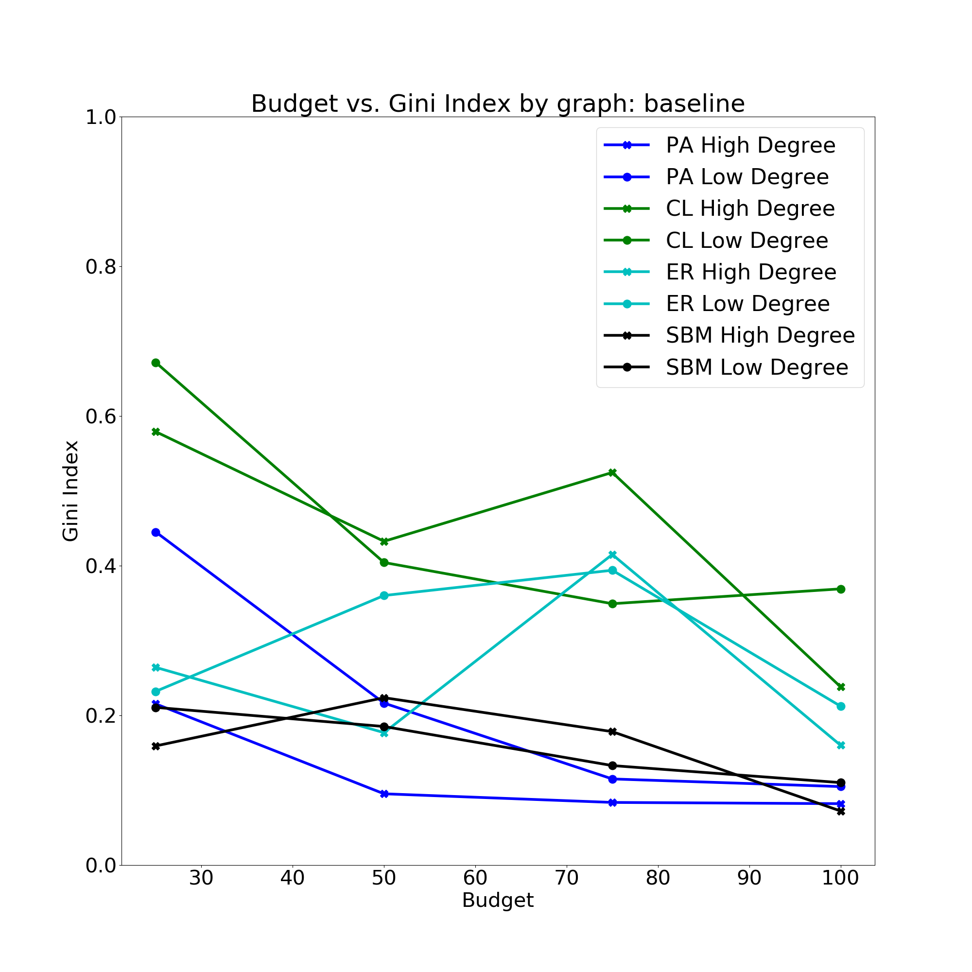
(a) GECI baseline

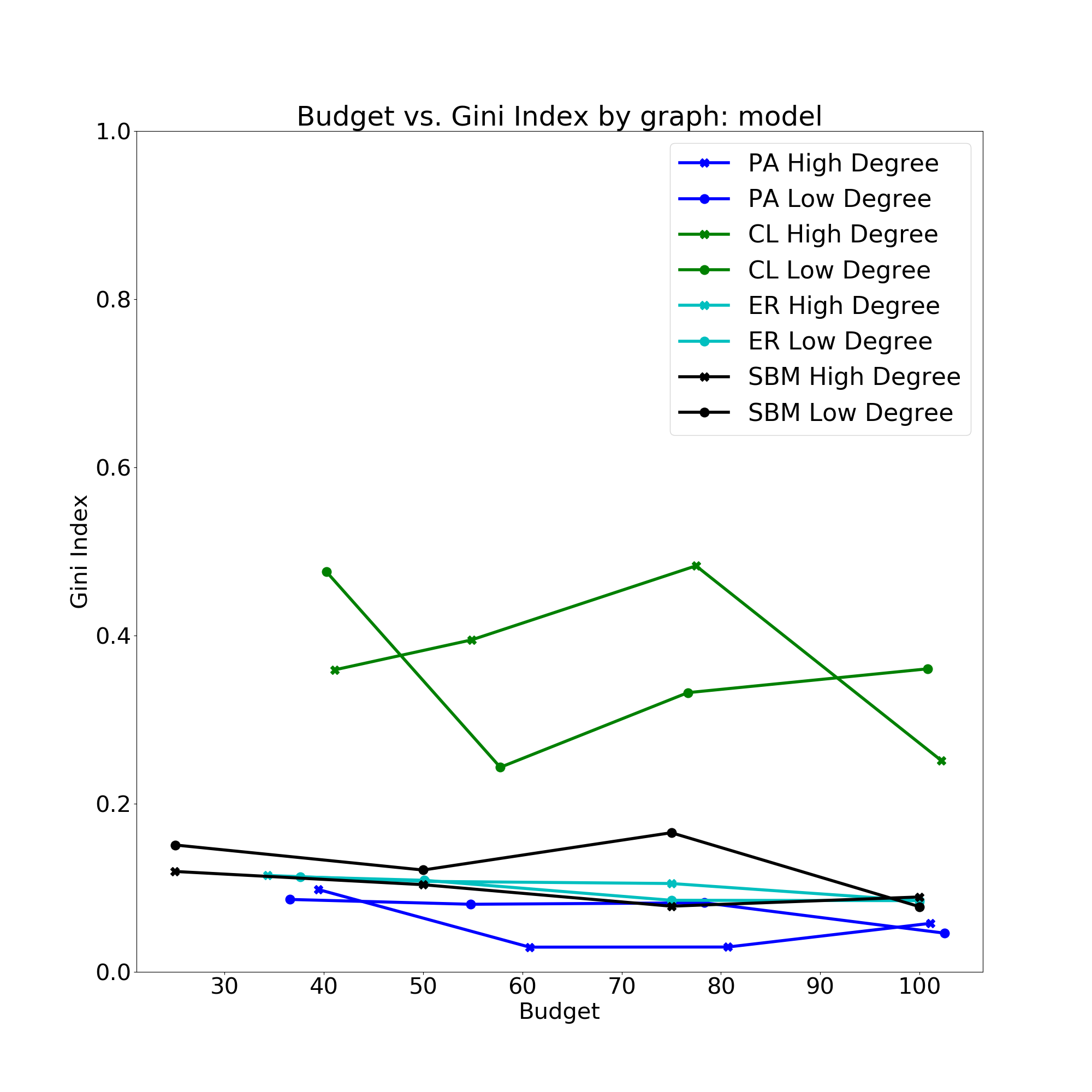
(b) Proposed method

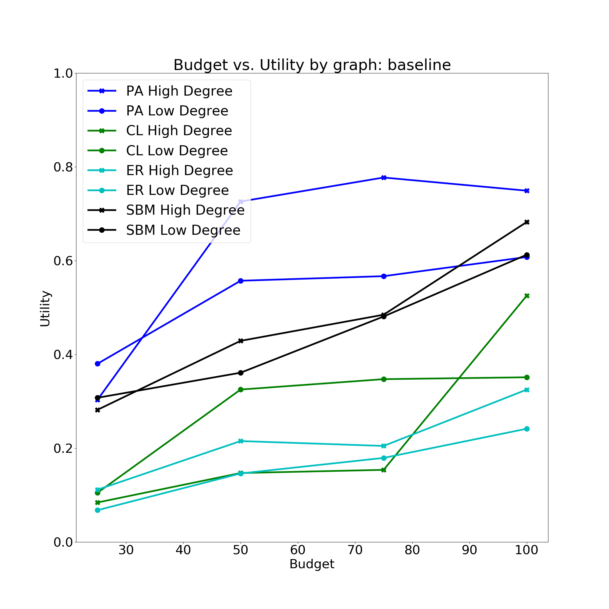
(c) GECI baseline

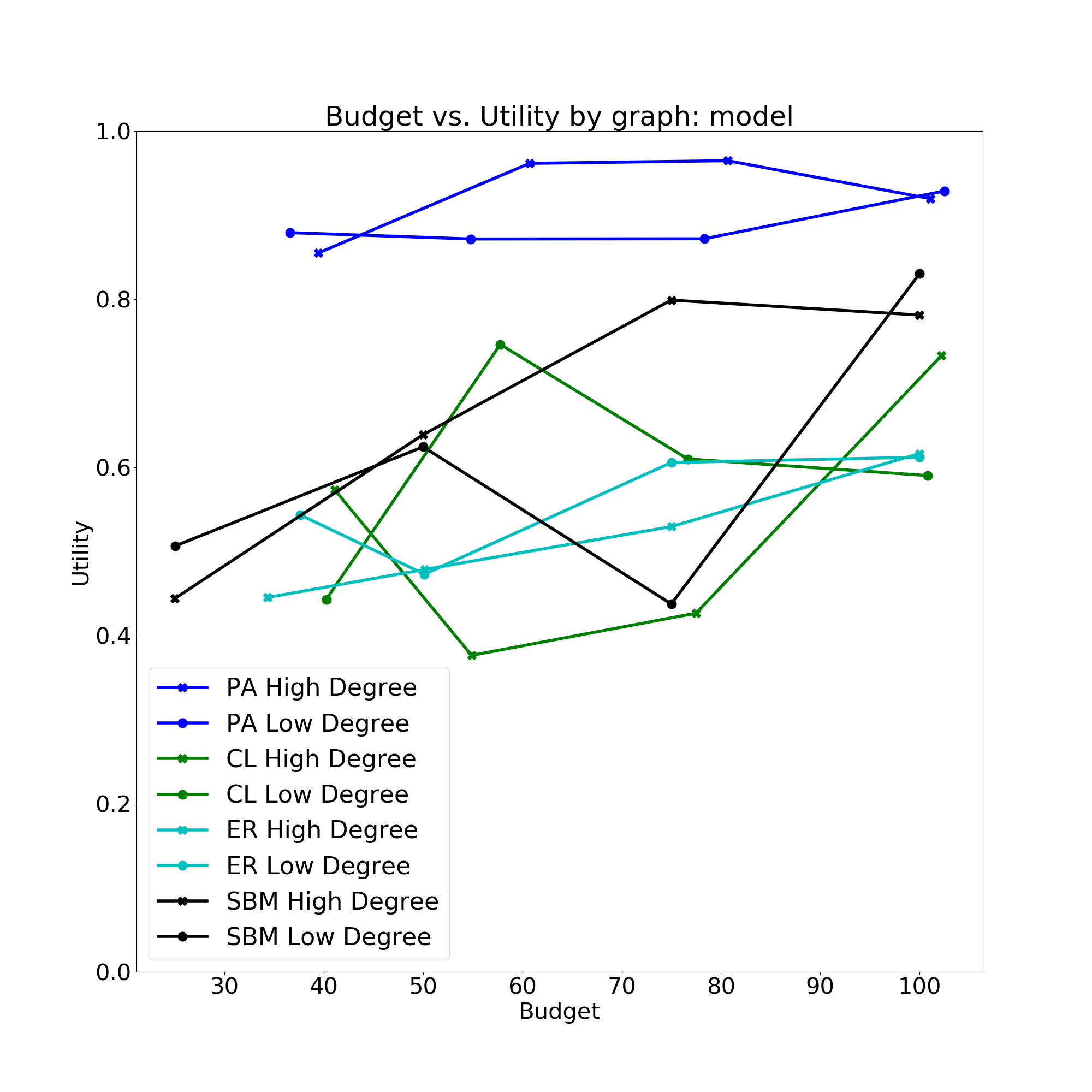
(d) Proposed model

Figure 3: (a-b) Budget vs Gini Index. This shows the Gini Index for varying budgets for (a) the GECI baseline and (b) our proposed method. Our proposed model performs better, particularly at a smaller budget. (c-d) Budget vs Utility. This shows the utility for varying budgets for (c) the GECI baseline and (d) our proposed method. Our proposed method outperforms the deterministic baseline on all graphs at all budgets.

Evaluation

We evaluate equity and utility for the graph produced by our method, comparing against the input graph and the baseline editing method. To define utility, we estimate the expected reward per group by repeated Monte Carlo sampling of weighted walks through the graph. First, we sample the starting node of an individual with respect to their initial distribution, then estimate their expected reward over weighted walks from the starting node. Repeatedly sampling individuals yields an expected utility for the graph with respect to each group. We measure the total expected reward per population (utility), and the difference in expected reward between classes (equity). Further, while our model only optimizes the expectation, it performs surprisingly well at minimizing the Gini Index.

Evaluation Metrics

Average Reward

We measure three graphs in experiments: the initial graph before editing, and outputs of the GECI baseline and our proposed method. We simulate 5000 weighted walks by the initial distributions of each particle type. Average reward is aggregated across these particle types.

Gini Index

The Gini Index is a measure of inequality. It measures the cumulative proportion of a population vs. the cumulative share of value (e.g. reward) for the population. At equality, the cumulative fraction of the population is equal to the cumulative reward. The measure is the deviation from this $x=y$ line, with $1$ being total inequality, and $0$ total equality.

Synthetic Results

Figure 3 overviews our synthetic results. We see that on all graphs and over almost all budgets, the proposed model outperforms the baseline. Further, we especially see that in the low-budget scenario, our model outperforms on Gini Index. Our model outperforms the baseline as much as $0.5$ in utility under the same budget. In particular, PA and ER graphs improve the most. Figure 4 gives the main empirical result of our synthetic experiments. On the $8$ experiments of $4$ different synthetic graphs, we plot the utility vs. the Gini Index across Monte Carlo simulations of the original, baseline, and proposed method graphs. The bottom-right reflects the best performance. Notice the proposed model outperforms the baseline on all synthetic graphs. Particularly notable, the Chung-Lu Power Law graph is the worst performing original graph in terms of both utility and Gini Index. However, on the low-degree problem instance, our method nearly doubles the utility performance of the baseline.

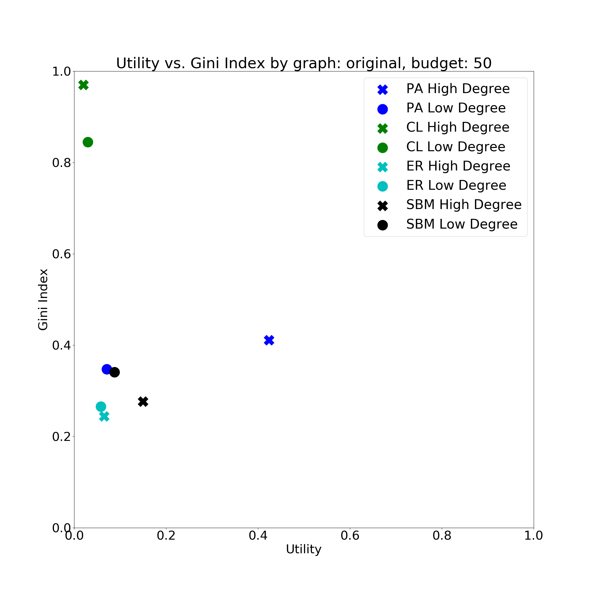
(a) Unedited Graph

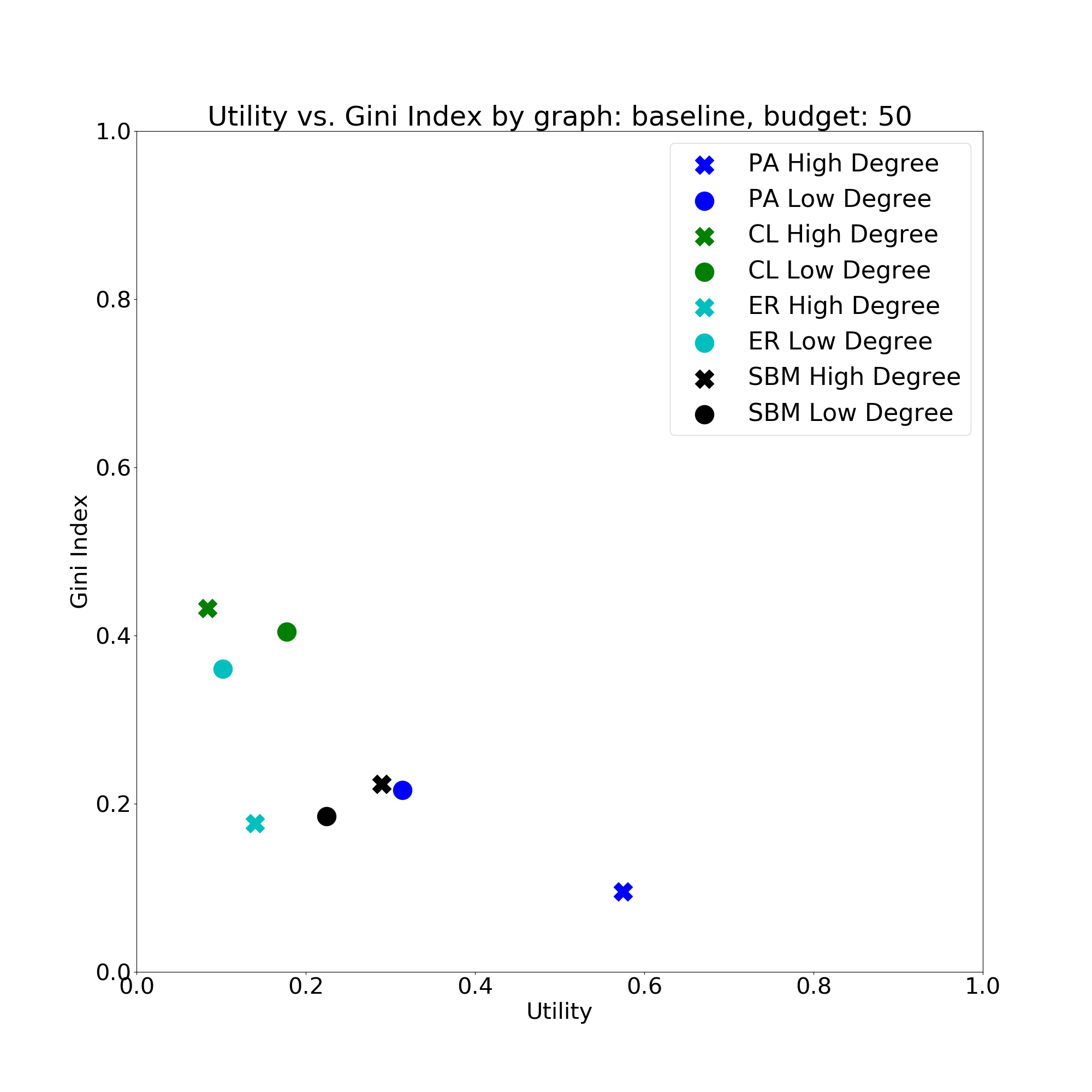
(b) GECI Baseline

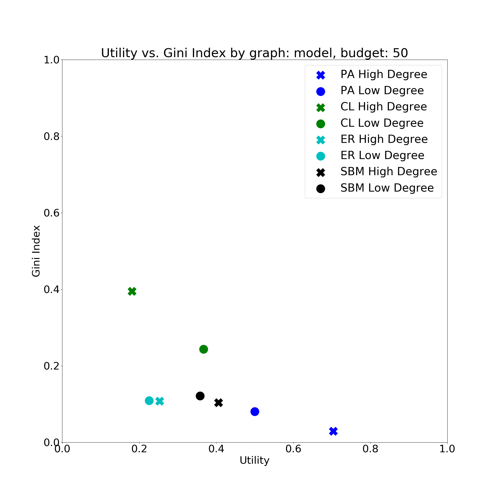
(c) Proposed method

Figure 4: A comparison of Utility vs. Gini Index across 8 synthetic experiments. Bottom-right is best. The proposed method performs best on all experiments.

Facility Placement

As discussed, our proposed model also solves the facility placement problem. The problem selects a number of nodes which maximizes the reward for particles sampled onto the graph from initial distributions. Figure 5 shows a simple experiment adapting our model for this problem. For brevity, we only show a small example experiment. In black, we see the curve of the Gini Index decreasing on increased budget of $15$ for a synthetic PA graph of size $|N|=200$. At the same time, the average utility increases to approximately the same budget. Note the initial location of PA high-degree under budget $3$ using the greedy PA high-degree heuristic (Figure 4(a)). This is approximately 4 for both Gini Index and Reward. Our method maintains far lower Gini Index. Therefore this node set largely covers the transition dynamics of the initial distributions.

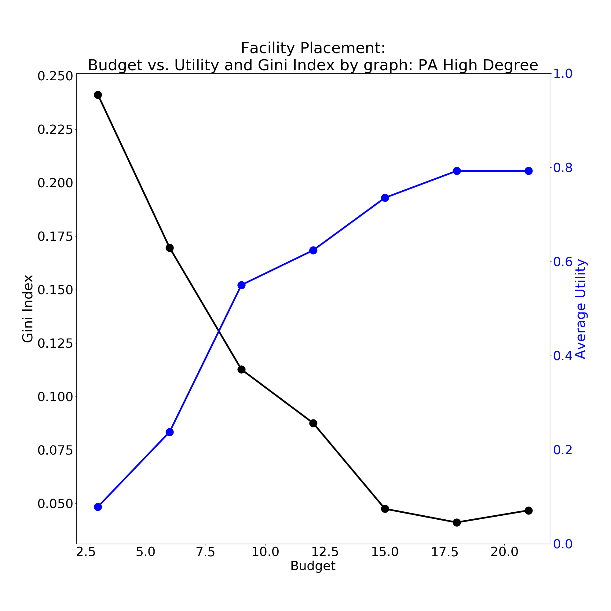
Figure 5: Facility placement results showing varying budget (facilities) vs. total Gini index and utility.

Chicago Schools
	Initial	GECI	Proposed Model
Avg. Utility	0.20	0.21	0.90
Gini Index	0.62	0.65	0.07

Table 1: Chicago Public School with budget 400

Real-World Applications

Equitable School Access in Chicago

In this section we study school inequity in the city of Chicago. We infer a coarse transportation network using the trajectory data of public bus lines from the Chicago Transit Authority (CTA). Nodes are given by route intersections, and edges are inferred from neighboring preceding and following intersections. This yields a graph with $2011$ nodes and $7984$ edges. We collect school location and quality evaluation data from the Chicago Public School (CPS) data portal. We use the $2018$-$2019$ School Quality Rating Policy assessment and select elementary or high schools with an assessment of ”Level 1+,” corresponding to “exceptional performance” of schools over the $90$th percentile. We select only non-charter, “network” schools which represent typical public schools. We use geolocation provided by CPS to create nodes within the graph. We attach these nodes to the graph using $2$-nearest neighbor search to the transportation nodes. Finally, we collect tract-level demographic data from the $2010$ census. We sample three classes of particle onto the network, representing White, Black, and Hispanic individuals by their respective empirical distribution over census tracts. We then randomly sample nodes within that tract to assign the particle’s initial position. We equally set initial edge weights for all groups, with weights inversely proportional to edge distance.

Table 1 shows the result for a budget of $400$ edges in the Chicago transportation network. We see that the baseline is surprisingly ineffective at increasing reward. Our method successfully optimizes for both utility and equity, achieving a very high performance on both metrics. Note that both the baseline and our proposed model make the same number of edits on the graph. We hypothesize the baseline performs poorly on graphs with a high diameter such as infrastructure graphs. Recall we similarly saw the baseline performs poorly on ER (Figure 4(b)), which has relatively dense routing. In contrast, our model learns the full reward function over the topology and can discover edits at the edge of its horizon.

Equitable Access in University Social Networks

To demonstrate the versatility of the proposed methods, we also apply them to reducing inequity in social networks. Social networks within universities and organizations may enable certain groups to more easily access people with valuable information or influence. We report experiments for university social networks using the Facebook100 data (Traud, Mucha, and Porter 2012).

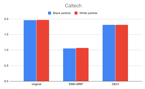
(a) Caltech.

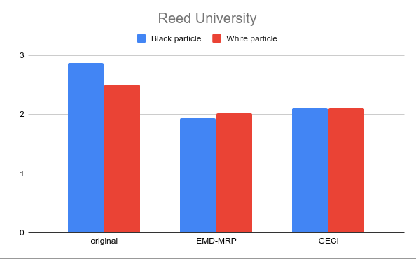
(b) Reed College.

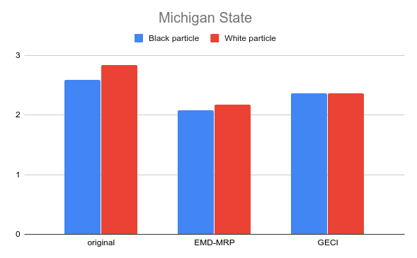
(c) Michigan State.

Figure 6: Mean shortest path of gender groups from the influence nodes

The Facebook100 dataset contains friendship networks at 100 US universities at some time in 2005. The node attributes of this network include: dorm, gender, graduation year, and academic major. Analyzing Facebook networks of universities yield sets of new social connections that would increase equitable access to certain attributed nodes across gender groups. We define popular seniors as the reward nodes and the objective is for freshmen of both genders to have equitable access to these influential nodes. In this experiment we mask the specific gender information by the term white and black particles. We demonstrate our method on three universities.

The results are in Figures 6(a), 6(b), and 6(c) which show the mean shortest path of gender groups from the influence nodes at Caltech, Reed College, and Michigan State University, respectively. Table 2 shows the intra-group Gini index. With sufficient hyperparameter tuning, our RL method within our novel MDP framework consistently outperforms the greedy GECI baseline on intra-group Gini index and minimizing overall shortest path of the freshman from the influence node across groups. On the other hand the difference between average shortest distance between groups, GECI maintains tighter margin when compared to our EMD-MRP approach. This is explained in the slackness in the constrained optimization of the EMD-MRP approach.

	Caltech	Reed	Mich. State
num. nodes, $|V|$	770	963	163806
num. edges, $|E|$	33312	37624	163806
num. editable edges $|A|$	336597	474439	3958660

Table 2: Graph properties of university social networks

	Original	EMD-MRP	GECI
Reed	0.214	0.093	0.153
Caltech	0.092	0.065	0.812
Michigan State	0.115	0.086	0.157

Table 3: Intra-group Gini Index

Conclusion

In this work, we proposed the Graph Augmentation for Equitable Access problem, which entails editing of graph edges, to achieve equitable diffusion dynamics-based utility across disparate groups. We motivated this problem through the application of equitable access in graphs, and in particular applications, equitable access in infrastructure and social networks. We evaluated our method on extensive synthetic experiments on 4 different synthetic graph models and 8 total experimental settings. We also evaluated on real-world settings.

There are many avenues for future work. First, our reward function is somewhat limiting. Ideally, individuals could collect rewards on the graph in a number of ways. Second, we measured a particular equal opportunity fairness which has a practical mapping to our application setting. However, other definitions of group or subgroup-level fairness may not be easily translatable to a graph routing/exploration problem.

Appendix

In this appendix, we provide some further details on the experiments in the main text.

Training Trajectories

Fig. 7 are the train trajectories on synthetic graphs. They indicate the trends of mean utility across, difference in utility across group and the budget constraint. The kinks in these learning curve are due to different scheduling schemes kicking in. Refer to Table 4 for these scheduling details for synthetic graph

(a) Mean Utility

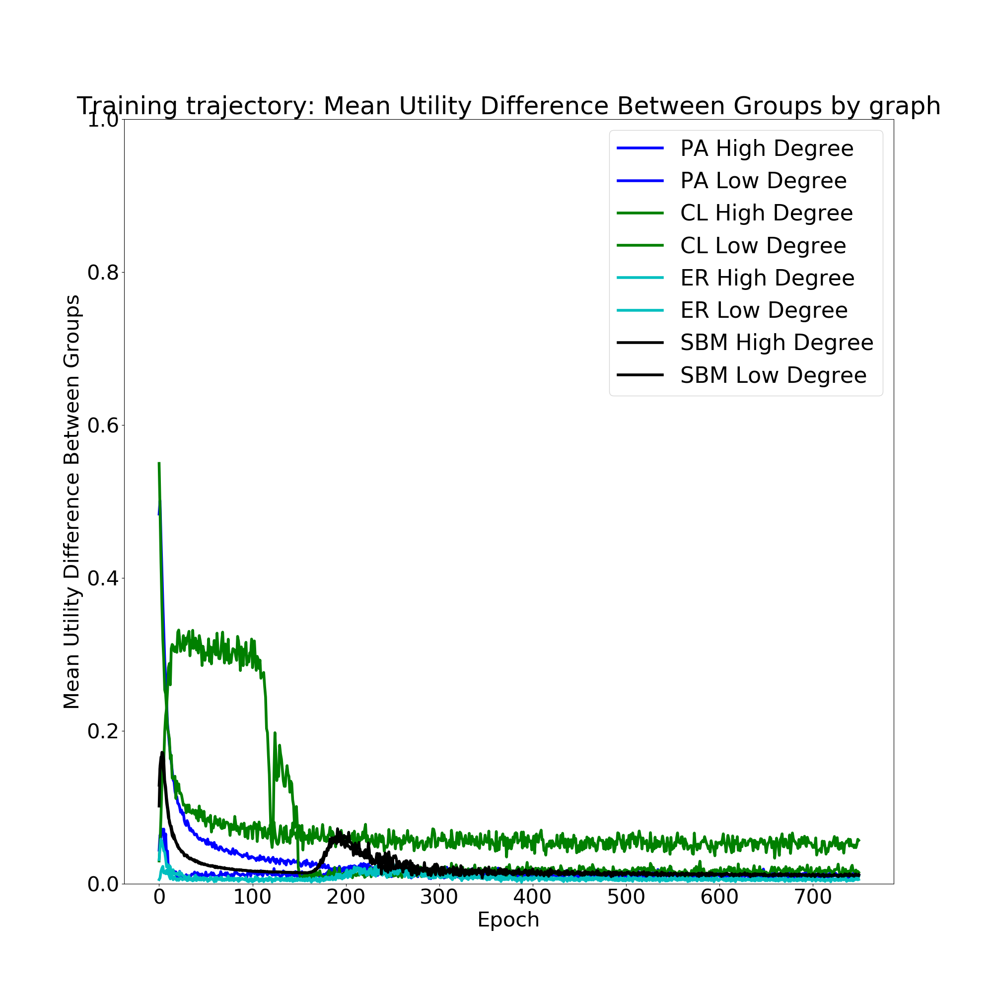
(b) Mean Utility Difference between groups

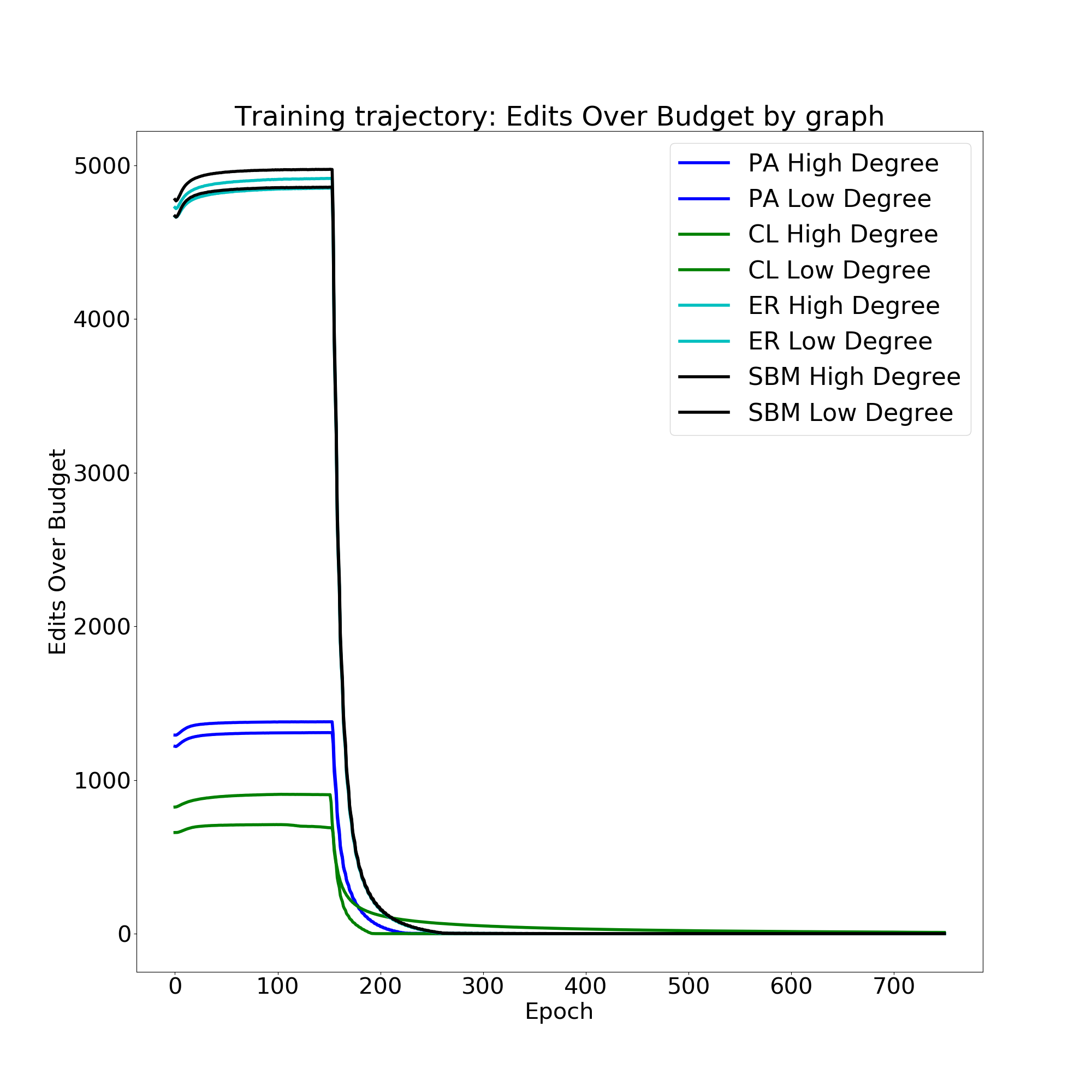
(c) Number of edits over budget

Figure 7: Training trajectories for the proposed model and the effect of training schedules are visualized.

Reproduciblity

Table 4 lists hyperparameters that were used for the different networks we experimented with.

.
	Synthetic Graphs	Road Networks	Social Networks
Budget, $B$	400	400	$0.2|V|$
Number of groups, $|G|$	2	3	2
MRP event horizon, $T$	10	10	3
Discount Factor, $\gamma$	0.99	0.99	0.7
Budget Lagrangian learning coefficient, $\mu_{1}$	$0.1$	$1$	$10000$
Equity Lagrangian learning coefficient, $\mu_{2}$	$1\times 10^{-6}$	$1\times 10^{-6}$	$1\times 10^{-6}$
Number of epochs, $E$	700	500	1000
Equity constraint schedule	$E>0$	$E>0$	$E>0$
Budget constraint schedule	$E>100$	$E>100$	$E>100$
Graph augmentation discretization schedule, $\tau\to\nu.\tau$	$E>200$	$E>200$	$E>300$
Temperature attenuation factor, $\nu$	0.999	0.995	0.995

Table 4: Hyperparameters used for different networks.

References

- Abebe et al. (2019) Abebe, R.; Immorlica, N.; Kleinberg, J.; and Lucier, B. 2019. Triadic Closure Alleviates Network Segregation. In Joint Workshop on AI for Social Good (NeurIPS ’19).
- Bowerman, Hall, and Calamai (1995) Bowerman, R.; Hall, B.; and Calamai, P. 1995. A multi-objective optimization approach to urban school bus routing: Formulation and solution method. Transportation Research Part A: Policy and Practice 29(2): 107–123. doi:10.1016/0965-8564(94)E0006-U.
- Carion et al. (2019) Carion, N.; Usunier, N.; Synnaeve, G.; and Lazaric, A. 2019. A Structured Prediction Approach for Generalization in Cooperative Multi-Agent Reinforcement Learning. In Wallach, H.; Larochelle, H.; Beygelzimer, A.; d'Alché-Buc, F.; Fox, E.; and Garnett, R., eds., Advances in Neural Information Processing Systems 32, 8128–8138. Curran Associates, Inc.
- Chung and Lu (2002) Chung, F.; and Lu, L. 2002. Connected components in random graphs with given expected degree sequences. Annals of Combinatorics 6(2): 125–145.
- Cole et al. (2018) Cole, M. J.; Bailey, R. M.; Cullis, J. D. S.; and New, M. G. 2018. Spatial inequality in water access and water use in South Africa. Water Policy 20(1): 37–52. doi:10.2166/wp.2017.111.
- Crescenzi et al. (2016) Crescenzi, P.; D’angelo, G.; Severini, L.; and Velaj, Y. 2016. Greedily improving our own closeness centrality in a network. ACM Transactions on Knowledge Discovery from Data 11(1): 1–32.
- Dwork and Ilvento (2018) Dwork, C.; and Ilvento, C. 2018. Fairness Under Composition. In 10th Innovations in Theoretical Computer Science Conference (ITCS 2019), 33:1–33:20. doi:10.4230/LIPIcs.ITCS.2019.33.
- Feige (1998) Feige, U. 1998. A threshold of for approximating set cover. Journal of the ACM 45(4): 634–652.
- Fish et al. (2019) Fish, B.; Bashardoust, A.; Boyd, D.; Friedler, S.; Scheidegger, C.; and Venkatasubramanian, S. 2019. Gaps in Information Access in Social Networks? In Proceedings of the World Wide Web Conference (WWW ’19), 480–490. doi:10.1145/3308558.3313680.
- Groeger, Waldman, and Eads (2018) Groeger, L. V.; Waldman, A.; and Eads, D. 2018. Miseducation: Is there racial inequality at your school? Retreived from https://projects.propublica.org/miseducation .
- Gupta et al. (2020) Gupta, S.; Jalan, A.; Ranade, G.; Yang; and Zhuang, S. 2020. Too Many Fairness Metrics: Is There a Solution? In Ethics of Data Science Conference. doi:10.2139/ssrn.3554829.
- Hay and Trinder (1991) Hay, A.; and Trinder, E. 1991. Concepts of Equity, Fairness, and Justice Expressed by Local Transport Policymakers. Environment and Planning C: Politics and Space 9(4): 453–465. doi:10.1068/c090453.
- Holland, Laskey, and Leinhardt (1983) Holland, P. W.; Laskey, K. B.; and Leinhardt, S. 1983. Stochastic blockmodels: First steps. Social Networks 5(2): 109–137.
- Holme and Kim (2002) Holme, P.; and Kim, B. J. 2002. Growing scale-free networks with tunable clustering. Physical Review E 65(2): 026107.
- Hsu and Ramachandran (1993) Hsu, T.-S.; and Ramachandran, V. 1993. Finding a Smallest Augmentation to Biconnect a Graph. SIAM Journal on Computing 22(5): 889–912. doi:10.1137/0222056.
- Jang, Gu, and Poole (2016) Jang, E.; Gu, S.; and Poole, B. 2016. Categorical reparameterization with Gumbel-softmax. arXiv:1611.01144 [stat.ML].
- Kempe, Kleinberg, and Tardos (2003) Kempe, D.; Kleinberg, J.; and Tardos, E. 2003. Maximizing the Spread of Influence through a Social Network. In Proceedings of the Ninth ACM SIGKDD International Conference on Knowledge Discovery and Data Mining (KDD ’03), 137–146. doi:10.1145/956750.956769.
- Le Gall (2014) Le Gall, F. 2014. Powers of tensors and fast matrix multiplication. In Proceedings of the 39th International Symposium on Symbolic and Algebraic Computation, 296–303.
- Leskovec et al. (2007) Leskovec, J.; Krause, A.; Guestrin, C.; Faloutsos, C.; VanBriesen, J.; and Glance, N. 2007. Cost-Effective Outbreak Detection in Networks. In Proceedings of the 13th ACM SIGKDD International Conference on Knowledge Discovery and Data Mining (KDD ’07), 420–429. doi:10.1145/1281192.1281239.
- Li et al. (2018) Li, Y.; Fan, J.; Wang, Y.; and Tan, K. 2018. Influence Maximization on Social Graphs: A Survey. IEEE Transactions on Knowledge and Data Engineering 30(10): 1852–1872. doi:10.1109/TKDE.2018.2807843.
- Littman (1994) Littman, M. L. 1994. Markov games as a framework for multi-agent reinforcement learning. In Machine learning proceedings 1994, 157–163. Elsevier.
- Logan (2014) Logan, J. 2014. Diversity and Disparities: America Enters a New Century. Russell Sage Foundation.
- Malakar, Mishra, and Patwardhan (2018) Malakar, K.; Mishra, T.; and Patwardhan, A. 2018. Inequality in water supply in India: an assessment using the Gini and Theil indices. Environment, Development and Sustainability 20: 841–864. doi:10.1007/s10668-017-9913-0.
- Mandell (1991) Mandell, M. B. 1991. Modelling Effectiveness-Equity Trade-Offs in Public Service Delivery Systems. Management Science 37(4): 377–499. doi:10.1287/mnsc.37.4.467.
- Marsh and Schilling (1994) Marsh, M. T.; and Schilling, D. A. 1994. Equity measurement in facility location analysis: A review and framework. European Journal of Operational Research 74(1): 1–17. doi:10.1016/0377-2217(94)90200-3.
- McAllister (1976) McAllister, D. M. 1976. Equity and Efficiency in Public Facility Location. Geographical Analysis 8(1): 47–63. doi:10.1111/j.1538-4632.1976.tb00528.x.
- Mehrabi et al. (2019) Mehrabi, N.; Morstatter, F.; Saxena, N.; Lerman, K.; and Galstyan, A. 2019. A survey on bias and fairness in machine learning. arXiv:1908.09635 [cs.LG].
- Mumphrey, Seley, and Wolpert (1971) Mumphrey, A. J.; Seley, J. E.; and Wolpert, J. 1971. A Decision Model for Locating Controversial Facilities. Journal of the American Institute of Planners 37(6): 397–402. doi:10.1080/01944367108977389.
- Nocedal and Wright (2006) Nocedal, J.; and Wright, S. 2006. Numerical Optimization. Springer Science & Business Media.
- Nowzari, Preciado, and Pappas (2016) Nowzari, C.; Preciado, V. M.; and Pappas, G. J. 2016. Analysis and Control of Epidemics: A Survey of Spreading Processes on Complex Networks. IEEE Control Systems Magazine 36(1): 26–46. doi:10.1109/MCS.2015.2495000.
- Orsi, Margellos-Anast, and Whitman (2010) Orsi, J. M.; Margellos-Anast, H.; and Whitman, S. 2010. Black–White Health Disparities in the United States and Chicago: A 15-Year Progress Analysis. American Journal of Public Health 100(2): 349–356. doi:10.2105/AJPH.2009.165407.
- Traud, Mucha, and Porter (2012) Traud, A. L.; Mucha, P. J.; and Porter, M. A. 2012. Social structure of Facebook networks. Physica A: Statistical Mechanics and its Applications 391(16): 4165–4180. doi:10.1016/j.physa.2011.12.021.
- Verma and Rubin (2018) Verma, S.; and Rubin, J. 2018. Fairness Definitions Explained. In 2018 IEEE/ACM International Workshop on Software Fairness (FairWare). doi:10.23919/FAIRWARE.2018.8452913.
- Xiao and Boyd (2004) Xiao, L.; and Boyd, S. 2004. Fast linear iterations for distributed averaging. Systems & Control Letters 53(1): 65–78.
- Youn, Gastner, and Jeong (2008) Youn, H.; Gastner, M. T.; and Jeong, H. 2008. Price of Anarchy in Transportation Networks: Efficiency and Optimality Control. Physical Review Letters 101(12): 128701. doi:10.1103/PhysRevLett.101.128701.
- Zhang et al. (2019) Zhang, Y.; Ramanathan, A.; Vullikanti, A.; Pullum, L.; and Prakash, B. A. 2019. Data-driven efficient network and surveillance-based immunization. Knowledge and Information Systems 61(3): 1667–1693. doi:10.1007/s10115-018-01326-x.
- Zheng et al. (2020) Zheng, S.; Trott, A.; Srinivasa, S.; Naik, N.; Gruesbeck, M.; Parkes, D. C.; and Socher, R. 2020. The AI Economist: Improving Equality and Productivity with AI-Driven Tax Policies. arXiv:2004.13332 [econ.GN].