Resonant four-photon scattering of collinear laser pulses in plasma

Abstract

Exact four-photon resonance of collinear planar laser pulses is known to be prohibited by the classical dispersion law of electromagnetic waves in plasma. We show here that the renormalization produced by an arbitrarily small relativistic electron nonlinearity removes this prohibition. The laser frequency shifts in collinear resonant four-photon scattering increase with laser intensities. For laser pulses of frequencies much greater than the electron plasma frequency, the shifts can also be much greater than the plasma frequency and even nearly double the input laser frequency at still small relativistic electron nonlinearities. This may enable broad range tunable lasers of very high frequencies and powers. Since the four-photon scattering does not rely on the Langmuir wave, which is very sensitive to plasma homogeneity, such lasers would also be able to operate at much larger plasma inhomogeneities than lasers based on stimulated Raman scattering in plasma.

I Introduction

Resonant interactions of collinear waves are particularly important because collinear wave packets are less susceptible to transverse slippage and could overlap longer, thus facilitating significant nonlinear transformations at relatively small intensities. However, low order resonant interactions of collinear waves may be forbidden for some classes of wave frequency dependence on wave number, $\omega(k)$.

In particular, the synchronism conditions for resonant two-into-two wave scattering of collinear waves read

$$k_{1}+k_{2}=k_{3}+k_{4}\,,$$ (1)

$$\omega_{1}+\omega_{2}=\omega_{3}+\omega_{4}\,,\;\;\;\omega_{j}=\omega(k_{j}),\;\;\;j=1,2,3,4.$$ (2)

These reduce, by a simple change of variables

$$k_{1}=k+q_{1}\,,\;\;k_{2}=k-q_{1}\,,\;\;k_{3}=k+q_{3}\,,\;\;k_{4}=k-q_{3}\,,$$ (3)

to the equation

$$f(k,q_{1})=f(k,q_{3})\,,\;\;\;f(k,q)=\omega(k+q)+\omega(k-q)\,.$$ (4)

For a monotonic in $q$ function $f(k,q)$, Eq. (4) has only the trivial solution $q_{3}=q_{1}$, for which output waves are identical with input waves, so that there is no “real” scattering.

In principle, even an arbitrarily small nonlinearity could cause a non-zero shift between wave numbers of output and input waves, thus enabling a real scattering. We will explore this possibility for the relativistic electron nonlinearity of electromagnetic waves in plasma.

The classical dispersion law for electromagnetic waves of physically “infinitely small” amplitudes in plasma is

$$\omega(k)=\sqrt{c^{2}k^{2}+\omega_{e}^{2}}\,,\;\;\;\;\omega_{e}=\sqrt{4\pi n_{0}e^{2}/m}\,,$$ (5)

where $c$ is the speed of light in vacuum, $m$ is the electron rest mass, $-e$ is the electron charge, and $n_{0}$ is the electron concentration of plasma. Under the convention $k>0$, $k_{1}>k_{2}$ and $k_{3}>k_{4}$, both $q_{1}$ and $q_{3}$ are by definition positive. For $q>0$ and $\omega(k)$ given by Eq. (5),

$$\frac{\partial f(k,q)}{c^{2}\partial q}=\frac{k+q}{\omega(k+q)}-\frac{k-q}{\omega(k-q)}>0\,,$$ (6)

so that $f(k,q)$ is a monotonically increasing function of $q>0$, which prohibits non-trivial resonant collinear four-photon scattering.

The renormalized resonant process to be explored could remove this prohibition by producing non-zero opposite frequency shifts of pulses 1 and 2. We will conventionally call the scattering “up-shifting” if it shifts up the higher frequency $\omega_{1}$, as schematically shown on the right Fig. 1, or “down-shifting” if it shifts down the higher frequency $\omega_{1}$, as on the left Fig. 1.

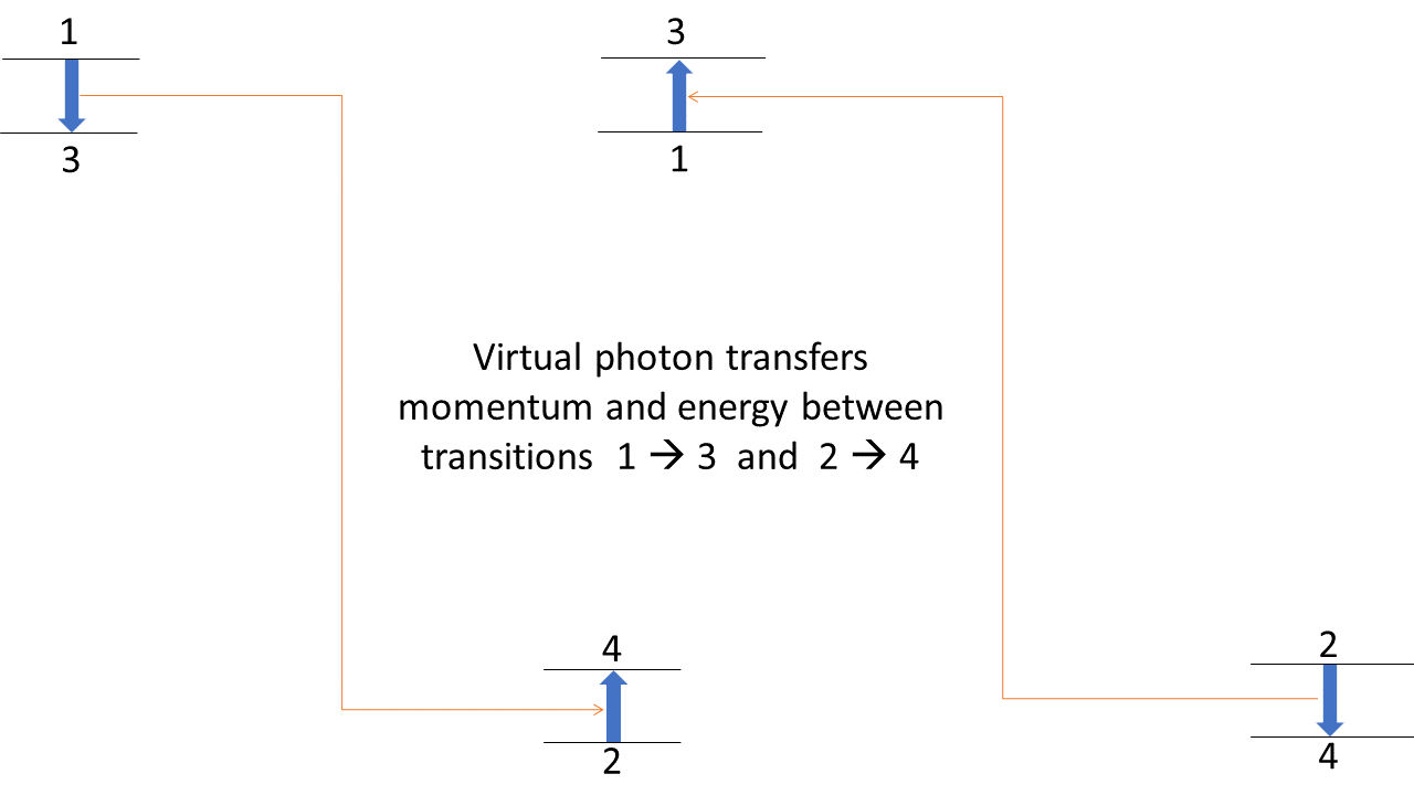
Figure 1: Opposite transitions of the input photons 1 and 2 into the output photons 3 and 4, respectively, coupled via a virtual photon exchange.

The dispersion law Eq. (5) prohibits also a photon decay into two or three photons. A photon may decay into a photon and electrostatic Langmuir wave of frequency close to the plasma frequency $\omega_{e}$. This process, called resonant stimulated Raman scattering, received significant attention 1974-PhysFluids-Drake-ParamInstEMWavesPlasma ; 1975-PhysFuids-Forslund-laser-scattering ; 1983-PhysFluids-Estabrook-Kruer ; 1992-PhysFluidsB-McKinstrie-SRFS-RelModul ; 1992-PRL-Antonsen-Mora ; 1993-PhysFluidsB-Antonsen-Mora . We will assume that the Raman scattering is suppressed, which could relatively easily occur due to small inhomogeneities in plasma frequency, detuning the resonance, or due to a longitudinal slippage between the electromagnetic and electrostatic waves having very different group velocities.

II Nonlinear Evolution Equation

To facilitate the forthcoming calculations, we will use the nonlinear evolution equation for dimensionless vector-potential $\boldsymbol{a}=e\boldsymbol{A}/mc^{2}$ of electromagnetic field derived in 2020-PRE-Malkin-4photonMJlasers . This general equation is much simplified in the special case of plane waves propagating along the axis $z$ and polarized along the axis $x$, so that $\boldsymbol{a}=a\boldsymbol{e_{x}}$,

$$(\partial^{2}_{t}-c^{2}\partial^{2}_{z}+\omega_{e}^{2}){a}=$$ (7)

$$\omega_{e}^{2}{a}[1-(\partial^{2}_{t}+\omega_{e}^{2})^{-1}c^{2}\partial_{zz}]a^{2}/2+O(a^{5}).$$

Though structurally similar to averaged cubic nonlinear wave equations, Eq. (7) does not assume any space or time averaging and, therefore, is applicable even for sets of laser pulses of very different wavelengths and frequencies, in contrast to the averaged wave equations used for describing stimulated Raman scattering of laser pulses in plasma 1974-PhysFluids-Drake-ParamInstEMWavesPlasma ; 1975-PhysFuids-Forslund-laser-scattering ; 1983-PhysFluids-Estabrook-Kruer ; 1992-PhysFluidsB-McKinstrie-SRFS-RelModul ; 1992-PRL-Antonsen-Mora ; 1993-PhysFluidsB-Antonsen-Mora .

For completeness, we give here a simplified derivation of Eq. (7). The derivation starts from the Maxwell equations in Coulomb gauge and Hamilton-Jacobi equation for electron motion in electromagnetic fields LandauLifshitz-ClassicalTheoryFields-1975-ch3 (kinetic effects are neglected, because all the beating phase velocities and electron quiver velocities considered here are much larger than electron thermal velocities):

$$\boldsymbol{H}=\nabla\times\boldsymbol{A},\quad\boldsymbol{E}=-\partial_{ct}\boldsymbol{A}-\nabla\Phi,\quad\nabla\cdot\boldsymbol{A}=0,$$ (8)

$$\Box\boldsymbol{A}\equiv\partial^{2}_{ct}\boldsymbol{A}-\Delta\boldsymbol{A}=4\pi\boldsymbol{J}/c-\partial_{ct}\nabla\Phi,$$ (9)

$$\boldsymbol{J}=-en\boldsymbol{P}/\sqrt{m^{2}+P^{2}/c^{2}},\quad\Delta\Phi=4\pi e(n-n_{0}),$$ (10)

$$\!\!\!\!\!\boldsymbol{P}=e\boldsymbol{A}/c+\nabla S,\;\;\partial_{t}S=e\Phi-c\sqrt{m^{2}c^{2}+P^{2}}+mc^{2}.\!$$ (11)

For dimensionless electromagnetic potentials, electron momentum and action,

$$\!\boldsymbol{A}=mc^{2}\boldsymbol{a}/e,\;\,\Phi=mc^{2}\phi/e,\;\,\boldsymbol{P}=mc\boldsymbol{p},\;\,S=mc^{2}s,\!\!\!$$ (12)

the equations can be reduced to the form

$$c^{2}\Box\boldsymbol{a}=-\boldsymbol{p}(1+p^{2})^{-1/2}(\omega_{e}^{2}+c^{2}\Delta\phi)-c\partial_{t}\nabla\phi,$$ (13)

$$\nabla\cdot\boldsymbol{a}=0,\;\;\boldsymbol{p}=\boldsymbol{a}+c\nabla s,\;\;\partial_{t}s=\phi-\sqrt{1+p^{2}}+1.$$ (14)

For collinear plane waves, all quantities depend, apart from on time, only on the longitudinal spacial variable $z$. Then, according to the equation $\nabla\cdot\boldsymbol{a}=0$, $\boldsymbol{a}$ has zero $z$-component, and Eqs. (13)-(14) take the form

$$\left[\partial^{2}_{t}-c^{2}\partial^{2}_{z}+\frac{\omega_{e}^{2}+c^{2}(\partial^{2}_{z}\phi)}{\sqrt{1+a^{2}+(c\partial_{z}s)^{2}}}\right]\boldsymbol{a}=0\,,$$ (15)

$$\frac{\omega_{e}^{2}+c^{2}(\partial^{2}_{z}\phi)}{\sqrt{1+a^{2}+(c\partial_{z}s)^{2}}}\,c\partial_{z}s+c\partial_{t}\partial_{z}\phi=0\,,$$ (16)

$$\partial_{t}s=\phi-\sqrt{1+a^{2}+(c\partial_{z}s)^{2}}+1\,.$$ (17)

For mildly relativistic electron quiver velocities in laser pulses, $a\ll 1$, Eqs. (15)-(17) can be expanded in powers of the small parameter $a$. To calculate the 4-photon coupling, the expansion should include terms up to cubic in $a$. In a uniform plasma, $\nabla\omega_{e}=0$, with the laser beatings well off the Raman resonance, and leading terms of the electrostatic potential $\phi$ and action $s$ expansions quadratic in $a$ (as will be immediately seen from the result), the expanded Eqs. (15)-(17) take the form

$$\left[\partial^{2}_{t}-c^{2}\partial^{2}_{z}+\omega_{e}^{2}(1-a^{2}/2)+c^{2}(\partial^{2}_{z}\phi)\right]\boldsymbol{a}=O(a^{5})\,,$$ (18)

$$\omega_{e}^{2}s+\partial_{t}\phi=O(a^{4})\,,$$ (19)

$$\partial_{t}s=\phi-a^{2}/2+O(a^{4})\,.$$ (20)

Exclusion of $s$ from Eqs. (19)-(20) gives the equation

$$(\partial^{2}_{t}+\omega_{e}^{2})\phi=a^{2}\omega_{e}^{2}/2+O(a^{4})\,,$$ (21)

which can be used now to exclude $\phi$ from Eq. (18),

$$(\partial^{2}_{t}-c^{2}\partial^{2}_{z}+\omega_{e}^{2})\boldsymbol{a}=$$ (22)

$$\boldsymbol{a}[1-c^{2}\partial^{2}_{z}(\partial^{2}_{t}+\omega_{e}^{2})^{-1}]a^{2}\omega_{e}^{2}/2+O(a^{5})\,.$$

For all waves polarized in the same direction, $\boldsymbol{a}=a\boldsymbol{e_{x}}$, Eq. (22) reduces to Eq. (7).

III Renormalized dispersion

For four-wave sets considered here,

$$a=\sum_{j=1}^{j=4}a_{j}\exp[\imath(k_{j}z-\omega_{j}t)]+c.c.+\delta a\,,$$ (23)

where $\delta a$ represents small non-resonant beatings generated by nonlinearity. For “infinitely small” pulses 3 and 4, $|a_{3}|,|a_{4}|\lll|a_{1}|,|a_{2}|$ , only pulses 1 and 2 contribute to renormalization of dispersion relations.

Substituting Eq. (23) in Eq. (7) and collecting all terms varying like $\exp[\imath(k_{j}z-\omega_{j}t)]$ lead to the following renormalized dispersion relations:

$$F_{j,l}=3-\frac{c^{2}(k_{j}-k_{l})^{2}}{(\omega_{j}-\omega_{l})^{2}-\omega_{e}^{2}}-\frac{c^{2}(k_{j}+k_{l})^{2}}{(\omega_{j}+\omega_{l})^{2}-\omega_{e}^{2}}\,,$$ (24)

$$c^{2}k_{1}^{2}+\omega_{e}^{2}-\omega_{1}^{2}\approx\omega_{e}^{2}\,\left(|a_{1}|^{2}F_{1,1}/2+|a_{2}|^{2}F_{1,2}\right)\,,$$

$$c^{2}k_{2}^{2}+\omega_{e}^{2}-\omega_{2}^{2}\approx\omega_{e}^{2}\,\left(|a_{2}|^{2}F_{2,2}/2+|a_{1}|^{2}F_{1,2}\right)\,,$$

$$c^{2}k_{3}^{2}+\omega_{e}^{2}-\omega_{3}^{2}\approx\omega_{e}^{2}\,\left(|a_{1}|^{2}F_{1,3}+|a_{2}|^{2}F_{2,3}\right)\,,\;\;\;$$

$$\;\;\;c^{2}k_{4}^{2}+\omega_{e}^{2}-\omega_{4}^{2}\approx\omega_{e}^{2}\,\left(|a_{1}|^{2}F_{1,4}+|a_{2}|^{2}F_{2,4}\right)\,.$$ (25)

These relations can be simplified for laser frequencies significantly exceeding the plasma frequency. The terms having sums of laser frequencies in denominators can be approximately replaced then by their vacuum value 1. Neglecting corrections containing extra small factors of order of $\omega_{e}^{2}/\omega_{j}^{2}$, Eqs. (24)-(25) reduce to:

$$F_{j,l}\approx 2-\frac{c^{2}(k_{j}-k_{l})^{2}}{(\omega_{j}-\omega_{l})^{2}-\omega_{e}^{2}}$$ (26)

$$\omega_{1}\approx ck_{1}+\frac{\omega_{e}^{2}}{2\omega_{1}}\left(1-|a_{1}|^{2}-|a_{2}|^{2}F_{1,2}\right),$$

$$\omega_{2}\approx ck_{2}+\frac{\omega_{e}^{2}}{2\omega_{2}}\left(1-|a_{2}|^{2}-|a_{1}|^{2}F_{1,2}\right),$$

$$\omega_{3}\approx ck_{3}+\frac{\omega_{e}^{2}}{2\omega_{3}}\left(1-|a_{1}|^{2}F_{1,3}-|a_{2}|^{2}F_{2,3}\right)\,,$$

$$\;\;\;\;\;\;\omega_{4}\approx ck_{4}+\frac{\omega_{e}^{2}}{2\omega_{4}}\left(1-|a_{1}|^{2}F_{1,4}-|a_{2}|^{2}F_{2,4}\right)\,.$$ (27)

IV Four-photon resonance

The renormalized dispersion law Eqs. (26)-(27) gives the following frequency mismatch in the temporal synchronism condition for four-photon scattering:

$$\delta\omega\equiv\omega_{1}+\omega_{2}-\omega_{3}-\omega_{4}\approx$$ (28)

$$\frac{\omega_{e}^{2}k(q_{1}^{2}-q_{3}^{2})}{ck_{1}k_{2}k_{3}k_{4}}(1-|a_{1}|^{2}-|a_{2}|^{2})+$$

$$\frac{\omega_{e}^{2}(k_{1}|a_{1}|^{2}+k_{2}|a_{2}|^{2})}{2ck_{1}k_{2}}\left(1-F_{1,2}\right)-$$

$$\frac{\omega_{e}^{2}|a_{1}|^{2}}{2ck_{3}k_{4}}\left[k_{3}(1-F_{1,4})+k_{4}(1-F_{1,3})\right]-$$

$$\frac{\omega_{e}^{2}|a_{2}|^{2}}{2ck_{3}k_{4}}\left[k_{3}(1-F_{2,4})+k_{4}(1-F_{2,3})\right]\,.$$

The four-photon resonance condition, $\delta\omega=0$, at which $F_{1,3}=F_{2,4}$ and $F_{2,3}=F_{1,4}$, can be presented in the form

$$2k(q_{1}^{2}-q_{3}^{2})\approx k_{3}k_{4}(k_{1}|a_{1}|^{2}+k_{2}|a_{2}|^{2})(F_{1,2}-1)+$$

$$k_{1}k_{2}(k_{4}|a_{1}|^{2}+k_{3}|a_{2}|^{2})(1-F_{1,3})+$$

$$k_{1}k_{2}(k_{3}|a_{1}|^{2}+k_{4}|a_{2}|^{2})(1-F_{1,4})\,.$$ (29)

For $|a_{2}|\approx|a_{1}|$, it simplifies to

$$(q_{1}^{2}-q_{3}^{2})/|a_{1}|^{2}\approx k_{3}k_{4}(F_{1,2}-1)-k_{1}k_{2}F\,,$$ (30)

$$F=F_{1,3}+F_{1,4}-2\,.$$ (31)

We will use this condition below to calculate the resonant manifold in the space of parameters $k$, $q_{1}$, $q_{3}$, $k_{e}\equiv\omega_{e}/c$ and $|a_{1}|$. But first, we will derive a general formula for the rate of the resonant four-photon scattering, in order to be able to calculate this rate right away in each regime.

V Four-photon scattering rate

The dominant terms producing scattering via the above four-photon resonance in Eq. (7) give the following evolution equations for very small slowly varying amplitudes of scattered pulses $3$ and $4$:

$$2\imath\omega_{3}\partial_{t}a_{3}\approx a_{1}a_{2}a_{4}^{*}\omega_{e}^{2}F,$$ (32)

$$2\imath\omega_{4}\partial_{t}a_{4}\approx a_{1}a_{2}a_{3}^{*}\omega_{e}^{2}F\,.$$ (33)

In the growing mode, the phases are synchronized as

$$\arg{a_{1}}+\arg{a_{2}}+\arg{F}=\arg{a_{3}}+\arg{a_{4}}+\pi/2,$$ (34)

and

$$|a_{3}|\sqrt{\omega_{3}}\approx|a_{4}|\sqrt{\omega_{4}}\propto\exp{\gamma t},$$ (35)

$$\gamma\approx\frac{\omega_{e}^{2}\,|Fa_{1}a_{2}|}{2\sqrt{\omega_{3}\omega_{4}}}.$$ (36)

VI Small resonant shift $|q_{3}-q_{1}|\ll k_{e}$

First, consider the resonance condition Eq. (30) in the limit $|a_{1}|\rightarrow 0$. Well off the Raman resonances, corresponding to zeros of $F_{1,j}$ denominators on the right hand side, it implies $q_{3}\rightarrow q_{1}$. Then, $k_{3}\rightarrow k_{1}$, $k_{4}\rightarrow k_{2}$, $F_{1,3}\rightarrow 2$, $F_{1,4}\rightarrow F_{1,2}$ and Eq. (30) reduces to

$$q_{3}^{2}-q_{1}^{2}\approx|a_{1}|^{2}\,k_{1}k_{2}\,.$$ (37)

As seen, $q_{3}>q_{1}$, so that the scattering up-shifts the photon 1, like in the scheme on the right Fig. 1. The scattering rate Eq. (36), with $F$ from Eqs. (31) and (26), in resonance Eq. (37), is

$$\gamma\approx\frac{\omega_{e}^{2}\,|a_{1}|^{2}}{2\sqrt{\omega_{1}\omega_{2}}}\left|\frac{(q_{1}+q_{3})^{2}-2k_{e}^{2}}{(q_{1}+q_{3})^{2}-k_{e}^{2}}\right|.$$ (38)

Thus, even an arbitrarily small relativistic electron nonlinearity enables non-trivial resonant collinear four-photon scattering with a non-zero frequency up-shift.

For regimes which are well off the Raman resonances at $q_{3}+q_{1}\approx k_{e}$ and $q_{1}\approx k_{e}/2$, formulas Eqs. (37)-(38) remain applicable as long as $q_{3}-q_{1}\ll k_{e}$, namely, at

$$|a_{1}|^{2}\ll\frac{k_{e}^{2}+2k_{e}q_{1}}{k_{1}k_{2}}\,.$$ (39)

VII Large resonant shift $|q_{3}-q_{1}|\gg k_{e}$

For $|q_{3}-q_{1}|\gg k_{e}$, Eqs. (30) and (36), supplemented by (26) and (31), approximately reduce to

$$\frac{q_{1}^{2}-q_{3}^{2}}{k_{e}^{2}|a_{1}|^{2}}\approx\frac{2k_{1}k_{2}(q_{1}^{2}+q_{3}^{2})}{(q_{1}^{2}-q_{3}^{2})^{2}}-\frac{k^{2}-q_{3}^{2}}{4q_{1}^{2}-k_{e}^{2}},$$ (40)

$$\gamma\approx\frac{ck_{e}^{4}\,|a_{1}|^{2}(q_{1}^{2}+q_{3}^{2})}{(q_{1}^{2}-q_{3}^{2})^{2}\,\sqrt{k^{2}-q_{3}^{2}}}\,.$$ (41)

Eq. (40) can be rewritten in the form

$$Y\approx\frac{X^{3}}{X^{2}-2QX-4Q}\,,\;\;\;\;Q=4-\frac{k_{e}^{2}}{q_{1}^{2}}\,,$$ (42)

$$X=\frac{q_{3}^{2}}{q_{1}^{2}}-1\,,\;\;\;\;Y=\frac{k_{1}k_{2}k_{e}^{2}|a_{1}|^{2}}{q_{1}^{2}(q_{1}^{2}Q+k_{e}^{2}|a_{1}|^{2})}\,.$$ (43)

For the down-shifting regimes, $q_{1}-q_{3}\gg k_{e}\Longrightarrow Q\approx 4$, Eqs. (42)-(43) approximately reduce to

$$\frac{k_{1}k_{2}k_{e}^{2}|a_{1}|^{2}}{4q_{1}^{4}}\approx Y\approx\frac{X^{3}}{X^{2}-8X-16}\,,\;\;\;X=\frac{q_{3}^{2}}{q_{1}^{2}}-1\,.$$ (44)

This resonant manifold is shown in the Fig. 2. As seen, $q_{3}/q_{1}$ increasing from 0 to 1 corresponds to $Y$ monotonically decreasing from $1/7$ to 0. The parameters need to satisfy the requirement

$$1\gg|a_{1}|^{2}\approx\frac{4q_{1}^{4}Y}{k_{1}k_{2}k_{e}^{2}}\,.$$ (45)

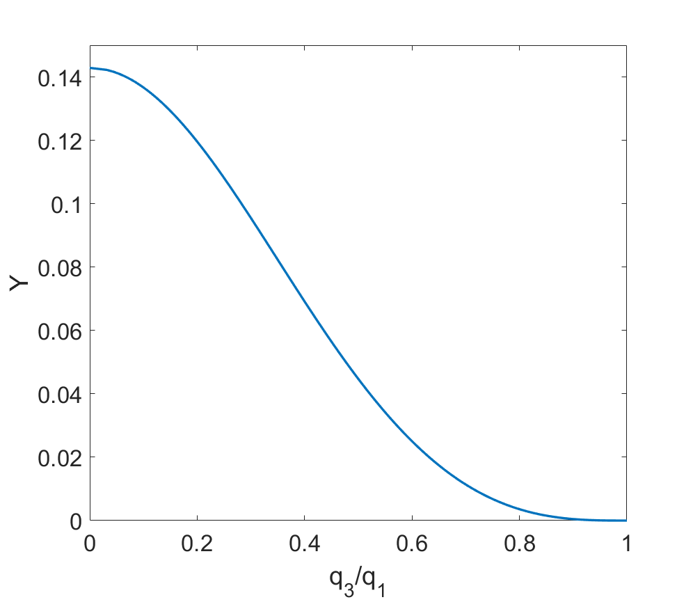
Figure 2: The resonant manifold Eq. (44) for down-shifting regimes $q_{1}-q_{3}\gg k_{e}$.

According to Eq. (44), at $k_{e}/q_{1}\ll 1-q_{3}/q_{1}\ll 1$

$$\frac{X}{2}\approx-\frac{q_{1}-q_{3}}{q_{1}}\,,\;\;\;\frac{k_{1}k_{2}k_{e}^{2}|a_{1}|^{2}}{4q_{1}^{4}}\approx Y\approx\frac{(q_{1}-q_{3})^{3}}{2q_{1}^{3}}\ll 1\,.$$

The down-shift is indeed much greater than the Raman scattering down-shift, $q_{1}-q_{3}\gg k_{e}$, at

$$|a_{1}|^{2}\gg\frac{2k_{e}q_{1}}{k_{1}k_{2}}\,.$$ (46)

The growth rate Eq. (41) at $1-q_{3}/q_{1}\ll 1$ is

$$\gamma\approx\frac{ck_{e}^{8/3}q_{1}^{2/3}|a_{1}|^{2/3}}{2^{1/3}(k_{1}k_{2})^{7/6}}\,.$$ (47)

As was schematically shown on the left in Fig. 1, the down-shifting four-photon scattering ($q_{3}<q_{1}$) makes photon wave-numbers closer to the average wave-number $k$. This tendency might be viewed as a dynamic counterpart of the tendency to Bose-Einstein condensation in kinetic regimes of four-wave scattering 1992-ZakharovLvovFalkovich-KolmogorovTurb ; 1996-PRL-Malkin ; 2015-PRE-Falkovich ; 2018-PRE-Malkin-OpticalTurb . The caveat is that all waves and beatings involved here are of the same nature. Otherwise, the tendency may change to up-shifting, like in the regime Eq. (37) where the four-photon scattering is noticeably mediated by quasi-electrostatic beatings.

For the up-shifting regimes, $q_{3}-q_{1}\gg k_{e}$, the resonant manifold given by Eqs. (42)-(43) is located at $Q>0$, $X>Q+\sqrt{Q^{2}+4Q}\,$. It is shown in the Fig. 3. At $X\gg 2+2Q$, Eq. (42) approximately reduces to $Y\approx X+2Q$.

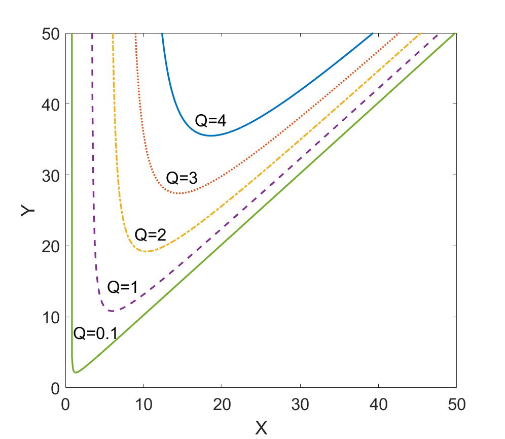
Figure 3: The resonant manifold Eq. (42) for up-shifting regimes $q_{3}-q_{1}\gg k_{e}$.

Eq. (43) can be rewritten in the form

$$Y=\frac{k_{1}k_{2}}{q_{1}^{2}(Z^{-1}+1)}\,,\;\;\;\;Z=\frac{k_{e}^{2}|a_{1}|^{2}}{q_{1}^{2}Q}>0\,.$$ (48)

For $X\gg 2+2Q$, when $Y\approx X\approx q_{3}^{2}/q_{1}^{2}\gg 1$, it follows

$$q_{3}\approx k/\sqrt{1+Z^{-1}}\,.$$ (49)

The parameters need to satisfy the requirement

$$1\gg|a_{1}|^{2}=(4q_{1}^{2}/k_{e}^{2}-1)Z\,.$$ (50)

The allowed $Z\ll(4q_{1}^{2}/k_{e}^{2}-1)^{-1}$ is small, $Z\ll 1$, at $4q_{1}^{2}/k_{e}^{2}-1\gtrsim 1$, but can be larger, $Z\gtrsim 1$, at $0<4q_{1}^{2}/k_{e}^{2}-1\ll 1$. To stay well off the Raman resonance at $2q_{1}\approx k_{e}$, having the width $|2q_{1}-k_{e}|\sim k_{e}^{2}|a_{1}|/2k$ in the regime $|a_{1}|\gg k_{e}/k$ of strongly coupled Stokes and anti-Stokes waves 1983-PhysFluids-Estabrook-Kruer ; 1992-PhysFluidsB-McKinstrie-SRFS-RelModul , it should be $Z^{-1}\gg k_{e}/k|a_{1}|$. This can be also put in the form $k_{4}=k-q_{3}\approx kZ^{-1}/2\gg k_{e}/2|a_{1}|$, or

$$|a_{1}|\gg k_{e}/2k_{4}\,.$$ (51)

The four-photon scattering rate Eq. (41) in the regime Eq. (49) is

$$\gamma\approx\frac{ck_{e}^{4}|a_{1}|^{2}(Z+1)^{3/2}}{k^{3}Z}\,.$$ (52)

For $Z\ll 1$, it reduces to

$$\gamma\approx\frac{ck_{e}^{4}|a_{1}|^{2}}{k^{3}Z}\approx\frac{ck_{e}^{2}(4q_{1}^{2}-k_{e}^{2})}{k^{3}}$$ (53)

and does not depend on the laser intensity. This behavior departs from that of the common four-wave scattering rate proportional to the wave intensity. It also departs from behavior of the modified rate Eq. (47) proportional to the cubic root of intensity as common for strongly coupled four-wave scattering regimes. The rate Eq. (53) contains the small factor $(4q_{1}^{2}-k_{e}^{2})/k^{2}$ instead of the common small factor proportional to intensity (apart from the factor $\omega_{e}^{2}/\omega$ common for all regimes).

For $1\ll Z\ll k|a_{1}|/k_{e}$, when the resonant four-photon scattering nearly doubles the laser frequency $k_{3}\equiv k+q_{3}\approx 2k-k/2Z$, the rate Eq. (52) reduces to

$$\gamma\approx\frac{ck_{e}^{4}|a_{1}|^{2}\sqrt{Z}}{k^{3}}\approx\frac{ck_{e}^{5}|a_{1}|^{3}}{k^{3}\sqrt{4q_{1}^{2}-k_{e}^{2}}}\,.$$ (54)

In contrast to the case Eq. (53), this rate depends on laser intensity even more strongly than does the common four-photon scattering rate.

The rate Eq. (52), as a function of $Z$, is minimal at $Z=2$, where

$$\gamma\approx\frac{3\sqrt{3}\,ck_{e}^{4}|a_{1}|^{2}}{2k^{3}}\,,\;\;\;\;k_{3}\approx 1.8k\,.$$ (55)

Even around this minimum, the rate can be sufficient to accomplish the scattering within small enough propagation distances.

For example, at $Z=1$, $k\approx 20\,k_{e}$ and $|a_{1}|^{2}\approx 0.1$, the resonant four-photon scattering produces the output laser pulse 3 of 1.7 the input laser frequency. The small-amplitude pulse 3 grows exponentially with the propagation distance and one exponentiation occurs within the length $c/\gamma\approx 9\times 10^{4}\,\lambda$. For the input laser wavelength of, say, $\lambda=1/3\,\mu$m, this length is $c/\gamma\approx 3$ cm.

VIII Summary

A new class of basic nonlinear processes has been identified, whereby collinear laser pulses can undergo an exactly resonant four-photon scattering, prohibited according to the classical dispersion law. The resonance is made possible by the intensity-dependent nonlinear frequency renormalization of the laser pulses. Despite being a higher order nonlinear process than the three-wave process of stimulated Raman scattering, the resonant renormalized four-photon scattering can occur in a relatively small propagation distance, so as to be of experimental interest in laboratory settings. Moreover, it can have important advantages over the stimulated Raman scattering:

• Because it does not rely on the Langmuir wave, which is very sensitive to plasma homogeneity, the four-photon scattering can tolerate much larger plasma inhomogeneities than can stimulated Raman scattering.

• Due to the smallness of longitudinal slippage between collinear laser pulses at large laser-to-plasma frequency ratios, the four-photon scattering can normally operate even for much shorter laser pulses than can stimulated Raman scattering.

• Frequency shifts produced by the resonant renormalized four-photon scattering can be tuned over a broad range by varying the intensity of the pulses, while the stimulated Raman scattering can shift the laser frequency only by the electron plasma frequency.

• For laser frequencies much greater than the electron plasma frequency, frequency shifts produced by the resonant renormalized four-photon scattering frequency can also be much greater than the electron plasma frequency at still just a mildly relativistic electron nonlinearity.

• The frequency shift can in fact be almost as large as the laser frequency, leading to output frequencies nearly twice the input frequency. The large frequency upshifts may enable an all-optical resonant frequency multiplication cascade in collinear geometry, which would be free of challenges associated with the transverse slippage of non-collinear laser pulses 2020-PRE-Malkin-4photonMJlasers .

IX Acknowledgment

The work is supported by Grants NNSA DENA0003871 and AFOSR FA9550-15-1-0391.

References

• (1) J. F. Drake, P. K. Kaw, Y. C. Lee, G. Schmid, C. S. Liu, and M. N. Rosenbluth, Parametric instabilities of electromagnetic waves in plasmas, The Physics of Fluids 17, 778–785 (1974).
https://doi.org/10.1063/1.1694789
• (2) D. W. Forslund, J. M. Kindel, and E. L. Lindman, Theory of stimulated scattering processes in laser-irradiated plasmas, The Physics of Fluids 18, 1002–1016 (1975).
https://doi.org/10.1063/1.861248
• (3) K. Estabrook and W. L. Kruer, Theory and simulation of one-dimensional Raman backward and forward scattering, The Physics of Fluids 26, 1892–1903 (1983).
https://doi.org/10.1063/1.864336
• (4) C. J. McKinstrie and R. Bingham, Stimulated Raman forward scattering and the relativistic modulational instability of light waves in rarefied plasma, Physics of Fluids B: Plasma Physics 4, 2626–2633 (1992).
https://doi.org/10.1063/1.860178
• (5) T. M. Antonsen and P. Mora, Self-focusing and Raman scattering of laser pulses in tenuous plasmas, Phys. Rev. Lett. 69, 2204–2207 (1992).
https://link.aps.org/doi/10.1103/PhysRevLett.69.2204
• (6) T. M. Antonsen and P. Mora, Self-focusing and Raman scattering of laser pulses in tenuous plasmas, Physics of Fluids B: Plasma Physics 5, 1440–1452 (1993).
https://doi.org/10.1063/1.860884
• (7) V. M. Malkin and N. J. Fisch, Towards megajoule x-ray lasers via relativistic four-photon cascade in plasma, Phys. Rev. E 101, 023 211 (2020).
https://doi.org/10.1103/PhysRevE.101.023211
• (8) L. D. Landau and E. M. Lifshitz, Chapter 3 - Charges in Electromagnetic Fields, in The Classical Theory of Fields (Fourth Edition) (Pergamon, Amsterdam, 1975), Vol. 2 of Course of Theoretical Physics, pp. 43 – 65.
https://doi.org/10.1016/B978-0-08-025072-4.50010-1
• (9) V. E. Zakharov, V. S. L’vov, and G. Falkovich, Kolmogorov spectra of turbulence 1. Wave turbulence (Springer, Berlin, 1992).
https://doi.org/10.1007/978-3-642-50052-7
• (10) V. M. Malkin, Kolmogorov and Nonstationary Spectra of Optical Turbulence, Phys. Rev. Lett. 76, 4524–4527 (1996).
https://doi.org/10.1103/PhysRevLett.76.4524
• (11) G. Falkovich and N. Vladimirova, Cascades in nonlocal turbulence, Phys. Rev. E 91, 041 201 (2015).
https://doi.org/10.1103/PhysRevE.91.041201
• (12) V. M. Malkin and N. J. Fisch, Transition between inverse and direct energy cascades in multiscale optical turbulence, Phys. Rev. E 97, 032 202 (2018).
https://doi.org/10.1103/PhysRevE.97.032202