Modeling the effects of dynamic range compression on signals in noise

Abstract

Hearing aids use dynamic range compression (DRC), a form of automatic gain control, to make quiet sounds louder and loud sounds quieter. Compression can improve listening comfort, but it can also cause distortion in noisy environments. It has been widely reported that DRC performs poorly in noise, but there has been little mathematical analysis of these distortion effects. This work introduces a mathematical model to study the behavior of DRC in noise. Using statistical assumptions about the signal envelopes, we define an effective compression function that models the compression applied to one signal in the presence of another. This framework is used to prove results about DRC that have been previously observed experimentally: that when DRC is applied to a mixture of signals, uncorrelated signal envelopes become negatively correlated; that the effective compression applied to each sound in a mixture is weaker than it would have been for the signal alone; and that compression can reduce the long-term signal-to-noise ratio in certain conditions. These theoretical results are supported by software experiments using recorded speech signals.

1 Introduction

Hearing aids often perform poorly where people with hearing loss need help most: in noisy environments with many competing sound sources. One challenge for hearing aids in noise is a nonlinear processing technique known as dynamic range compression (DRC), which makes quiet sounds louder and loud sounds quieter (Souza, 2002; Allen, 2003; Kates, 2005). Compression is used in all modern hearing aids, but it can cause distortion when applied to multiple overlapping signals. For example, a sudden loud noise can reduce the gain applied to speech sounds. This effect is well documented empirically, but has been little studied mathematically. To better understand the performance of DRC in noisy environments, this work applies tools from signal processing theory to model the effects of DRC on mixtures of multiple signals.

The auditory systems of people with hearing loss have reduced dynamic range compared to those of normal-hearing listeners: Quiet sounds need to be amplified in order to be audible, but loud sounds can cause discomfort. Hearing aids with DRC apply level-dependent amplification so that the output signal has a smaller dynamic range than the input signal. A typical DRC system is shown in Fig. 1. An envelope detector tracks the level of the input signal over time in one or more frequency bands while a compression function adjusts the amplification to keep the signal level within a comfortable range. Both the envelope detector and the compression function are nonlinear processes, so changes in one signal can affect the processing applied to other signals.

This interaction between signals can be difficult to measure, but hearing researchers have found three quantifiable effects of compression in noise. First, as one signal grows louder, it reduces the gain applied to the mixture, thereby lowering the level of the other signal(s) in the output. This effect has been called co-modulation (Stone and Moore, 2004) or across-source modulation (Stone and Moore, 2007). Second, noise can reduce the effect of a compressor, especially at low signal-to-noise ratios (SNR) (Souza et al., 2006). If one signal has much higher level than another, the DRC system will apply gain based on the stronger signal and will have little effect on the dynamic range of the weaker signal. Finally, at high SNR, compressors tend to amplify low-level noise more strongly than the higher-level signal of interest, which can reduce the average SNR (Souza et al., 2006; Rhebergen et al., 2009; Alexander and Masterson, 2015). This effect has been observed in commercial hearing aids and shown to impair speech comprehension (Naylor and Johannesson, 2009; Miller et al., 2017).

The adverse effects of noise on DRC systems have been well documented empirically, but the problem has received little mathematical analysis, which could provide more insight than empirical evidence alone. This work applies signal processing research methods to the DRC distortion problem: First, we make simplifying assumptions to develop a tractable mathematical model of a complex system. Next, we use that model to prove theorems that explain the behavior of the system. Finally, we validate those theoretical results using realistic experiments.

Figure 1: A typical DRC system performs automatic gain control in each of several frequency bands or channels.

Compression systems are difficult to analyze because of the complex interactions between the envelope detector and compression function, both of which are nonlinear. Using the simplifying assumption that envelopes are additive in signal mixtures, we can separate the effects of the envelope detector from those of the compression function. To characterize the interaction between signals in a mixture, we introduce the effective compression function (ECF), which relates the input and output levels of one signal in the presence of another. The ECF is used to explain the three effects described above: that compression induces negative correlation between signal envelopes (Section 4), that noise reduces the effect of compression (Section 5), and that compression can reduce average SNR in certain conditions (Section 6). Each section includes a theorem about the effect and simulation experiments that illustrate it. Wherever possible, these results are compared to those reported in the hearing literature.

2 Dynamic Range Compression of a Single Signal

Because most modern hearing aids are digital, we formulate the DRC system in discrete time. Let the sequence $\tilde{x}[t]$ be a sampled audio signal at the input of the DRC system, where $t$ is the sample index. Let $\tilde{y}[t]$ be the output of the system.

2.1 Filterbank decomposition

In hearing aids, DRC is often performed separately in several frequency bands. A filterbank splits the signal into $B$ channels corresponding to different bands, which may be uniform or nonuniform and may or may not overlap. Let $x[t,b]$ and $y[t,b]$ be the filterbank representations of $\tilde{x}[t]$ and $\tilde{y}[t]$, respectively, in channels $b=1,\dots,B$.

The number and structure of channels are known to have significant effects on the performance of DRC systems in noise (Naylor and Johannesson, 2009; Alexander and Masterson, 2015; Rallapalli and Alexander, 2019). The levels of signals in narrower bands fluctuate more rapidly than the levels of wideband signals, and so systems with more channels tend to compress signals more strongly and to produce greater distortion effects. The experiments in this work use a Mel-spaced filterbank with 6 bands, which are roughly uniformly spaced at lower frequencies and exponentially spaced at higher frequencies.

2.2 Envelope detection

The gain applied by DRC is calculated from the signal envelope, which tracks the signal level over time. Signal level is typically defined in terms of either magnitude ($|x|$) or power ($x^{2}$); this work uses power. Let the nonnegative signal $v_{x}[t,b]$ be the envelope of the input signal $x[t,b]$ at time index $t$ and channel $b$. In the theoretical analysis presented here, the envelope is an abstract property of a signal. For example, it can be thought of as the time-varying statistical variance of a random process of which the signal $x[t,b]$ is a realization. In real DRC systems, the envelope is estimated from the observed signal.

Because hearing aids must process signals with imperceptible delay, a practical envelope detector estimates signal level based on a moving average of past samples. Most DRC systems respond faster to increases in signal level (attack mode) than to decreases in signal level (release mode). Short attack times, typically a few milliseconds, help to suppress sudden loud sounds. Longer release times, from tens to hundreds of milliseconds, ensure that gain is not increased too quickly during brief pauses (Jenstad and Souza, 2005).

There are many ways of implementing an envelope detector (Giannoulis et al., 2012). A representative detector, which is used in the experiments throughout this work, is the nonlinear recursive filter (Kates, 2008)

$$v_{x}[t,b]=\begin{cases}\beta_{\text{a}}v_{x}[t\!-\!1,b]\!+\!(1\!-\!\beta_{\mathrm{a}})\left|x[t,b]\right|^{2},\\ &\text{if }\left|x[t,b]\right|^{2}\geq v_{x}[t\!-\!1,b]\\ \beta_{\text{r}}v_{x}[t\!-\!1,b]\!+\!(1\!-\!\beta_{\mathrm{r}})\left|x[t,b]\right|^{2},&\text{otherwise},\end{cases}$$ (1)

for $b=1,\dots,B,$ where $\beta_{\mathrm{a}}$ and $\beta_{\mathrm{r}}$ are constants that determine the attack and release times.

Because envelope detection is a nonlinear process, it contributes to the distortion effects of DRC systems. The theorems in this work do not depend directly on the choice of attack and release time, but these parameters do affect the distribution of envelope samples: A slowly-changing envelope detector will measure a narrower dynamic range than a fast-changing detector for the same signal. Many distortion effects are therefore more severe for fast-acting than for slow-acting compression (Jenstad and Souza, 2005; Naylor and Johannesson, 2009; Alexander and Masterson, 2015; Reinhart et al., 2017; Alexander and Rallapalli, 2017).

2.3 Compression function

Figure 2: A compression function $\mathcal{C}_{b}$, shown here on a logarithmic scale, maps input levels to output levels.

A compression function $\mathcal{C}_{b}$ determines the mapping between input and output level in each channel:

$$v_{y}[t,b]=\mathcal{C}_{b}\left(v_{x}[t,b]\right),\quad b=1,\dots,B,$$ (2)

where $v_{y}[t,b]$ is the target output level. The amplification applied in each channel is then

$$g[t,b]=\sqrt{\frac{v_{y}[t,b]}{v_{x}[t,b]}},\quad b=1,\dots,B,$$ (3)

so that the output is

$$y[t,b]=g[t,b]x[t,b],\quad b=1,\dots,B.$$ (4)

Note that the target output level $v_{y}[t,b]$ is not necessarily equal to the measured envelope of $y[t,b]$ because the envelope is a nonlinear moving average of present and past levels. Since this distinction is not important to our analysis, similar notation will be used for both.

Although compression functions are defined here in terms of input and output level (i.e., power), they are often visualized and described on a logarithmic scale, such as in dB SPL (sound pressure level). A typical “knee-shaped” compression function is shown in Fig. 2: It features a linear region in which gain is constant, a compressive region where the output level increases by less than the input level, and and a limiting region that prevents the output from exceeding a maximum safe level.

The strength of compression can be characterized by the compression ratio (CR), which is the inverse of the slope of the compression function on a log-log scale. For example, in a 3:1 compression system, the output level increases by 1 dB for every 3 dB increase in the input level. For a DRC system with constant compression ratio $\mathrm{CR}$, the compression function is given by the power-law relationship

$$\mathcal{C}_{b}(v)=g_{0}^{2}[b]v^{1/\mathrm{CR}},$$ (5)

where $g_{0}^{2}[b]$ is a constant gain factor. Thus, for a 3:1 compressor, the output level is proportional the cube root of the input level. In limiters, $\mathcal{C}_{b}(v)$ is constant and so the compression ratio is infinite.

While most compressors reported in the literature use some combination of linear, power-law, and limiting compression functions, many others are possible. For example, cascaded feedback systems can be used to design smoothly curved compression functions with roughly logarithmic shapes (Lyon, 2017). In digital systems, $\mathcal{C}_{b}$ can be arbitrary. To make our analysis as general as possible, we allow the compression function to be any mapping between nonnegative numbers such that the output level grows no faster than the input level.

Definition 1.

A function $\mathcal{C}_{b}(v)$ is a compression function if it is concave, nonnegative, and nondecreasing for all $v>0$.

To describe how much a compression function reduces the dynamic range of a signal, we could compute its compression ratio. Because the compression ratio can be infinite, however, it is more convenient to work with its inverse, the compression slope.

Definition 2.

For all points $v$ at which a compression function $\mathcal{C}_{b}(v)$ is differentiable, the compression slope $\mathrm{CS}_{b}(v)$ is the slope of $\mathcal{C}_{b}(v)$ on a log-log scale:

$$\mathrm{CS}_{b}(v) =\frac{\mathrm{d}}{\mathrm{d}u}\ln\mathcal{C}_{b}\left(e^{u}\right)\mid_{u=\ln v}$$ (6)

$$=\frac{\mathcal{C}^{\prime}_{b}(v)}{\mathcal{C}_{b}(v)}v.$$ (7)

For example, if $\mathcal{C}_{b}(v)=g_{0}^{2}[b]v^{\alpha}$, then $\mathrm{CS}_{b}(v)=\alpha$ for all $v$. The smaller the compression slope, the more the dynamic range of the signal is reduced.

3 Modeling Compression of Sound Mixtures

Figure 3: A simplified model separates the effects of the filterbank and envelope detector from those of the compression functions $\mathcal{C}_{b}$. The former is assumed to act independently across component signals, while the latter act independently across time and channels.

Hearing aids are often used in noisy environments with multiple sound sources. Because DRC is a nonlinear process, these signals interact and cause distortion. This distortion is especially difficult to analyze because DRC involves two nonlinear operations: envelope detection and level-dependent amplification. To create a tractable model, we make a simplifying assumption about the signal envelopes that allows us to separate the effects of these nonlinarities, as shown in Fig. 3. Under this model, the filterbank and envelope detector determine the relationship between input signals and envelope values; they are modeled as acting independently on each source signal. The compression function determines the output levels from these envelopes; it acts independently at each time index and within each channel.

3.1 Envelope model

Suppose that the input to the system is $\tilde{x}[t]=\tilde{s}_{1}[t]+\tilde{s}_{2}[t]$, where $\tilde{s}_{1}[t]$ and $\tilde{s}_{2}[t]$ are two discrete-time signals. Because a filterbank is a linear system, the filterbank representation of the input is

$$x[t,b]=s_{1}[t,b]+s_{2}[t,b],\quad b=1,\dots,B,$$ (8)

where $s_{1}[t,b]$ and $s_{2}[t,b]$ are the filterbank representations of $\tilde{s}_{1}[t]$ and $\tilde{s}_{2}[t]$, respectively.

Because envelope detection is a nonlinear process, the additivity property of Eq. (8) does not hold in general for the signal envelopes measured by practical envelope detectors. However, to simplify our analysis, the signal envelopes can be modeled as obeying additivity.

Assumption 1.

The envelopes $v_{s_{1}}[t,b]$, $v_{s_{2}}[t,b]$, and $v_{x}[t,b]$ of $s_{1}[t,b]$, $s_{2}[t,b]$, and $x[t,b]$ satisfy

$$v_{x}[t,b]=v_{s_{1}}[t,b]+v_{s_{2}}[t,b],\quad b=1,\dots,B.$$ (9)

To justify this assumption, suppose that $s_{1}[t,b]$ and $s_{2}[t,b]$ are sample functions of zero-mean random processes that are uncorrelated with each other. Then $\mathbb{E}\left[|x[t,b]|^{2}\right]=\mathbb{E}\left[|s_{1}[t,b]|^{2}\right]+\mathbb{E}\left[|s_{2}[t,b]|^{2}\right]$, where $\mathbb{E}$ denotes the statistical expectation. If $v_{x}[t,b]$ were any linear transformation of the sequence $\mathbb{E}\left[|x[t,b]|^{2}\right]$, then the envelopes would satisfy Assumption 1. This statistical model is useful because the instantaneous level $\left|x[t,b]\right|^{2}$ from Eq. (1) can be thought of as an estimator of the variance $\mathbb{E}\left[|x[t,b]|^{2}\right]$. If $\beta_{\mathrm{a}}=\beta_{\mathrm{r}}$, then the recursive filter would be a linear transformation of this estimator. This model does not reflect the peak-tracking behavior of envelope detectors with $\beta_{\mathrm{a}}\neq\beta_{\mathrm{r}}$. However, the simulation experiments in this work do include peak tracking.

3.2 Output model

Care is also required in analyzing the components of the output of a nonlinear system. Let $\tilde{y}[t]=\tilde{r}_{1}[t]+\tilde{r}_{2}[t]$, where $\tilde{r}_{1}[t]$ is the component of the output corresponding to $\tilde{s}_{1}[t]$ and $\tilde{r}_{2}[t]$ is the component corresponding to $\tilde{s}_{2}[t]$. For systems with the additivity property, like linear filters, these components can be calculated by applying the same system to $\tilde{s}_{1}$ and $\tilde{s}_{2}$. For nonlinear systems like DRC, each component of the output depends on both components of the input, so it can be difficult to meaningfully decompose the output into distinct components. For example, in certain musical genres, DRC is used to produce deliberately strong distortion so that the original signals are barely recognizable in the output. In hearing aids, however, the effects of DRC should be perceptually transparent: The distortion should be subtle enough that an approximate notion of additivity can apply.

In this work, the output components are determined by calculating the level-dependent amplification sequence $g[t,b]$ based on the mixture $x[t,b]$, then applying it to each component:

$$y[t,b] =g[t,b]x[t,b]$$ (10)

$$=g[t,b]\left(s_{1}[t,b]+s_{2}[t,b]\right)$$ (11)

$$=\underbrace{g[t,b]s_{1}[t,b]}_{r_{1}[t,b]}+\underbrace{g[t,b]s_{2}[t,b]}_{r_{2}[t,b]}$$ (12)

for all time indices $t$ and channels $b=1,\dots,B$. This decomposition is used in the mathematical analysis below. Similarly, in the software simulations presented here, the separate input signals are stored in memory alongside their mixture and the amplification sequence is applied separately to each, allowing the output components to be computed exactly. In laboratory experiments with real hearing aids, many researchers use a linearization technique known as phase inversion (Hagerman and Olofsson, 2004) to estimate the output components due to each source signal.

3.3 Effective compression function

Figure 4: Gain applied to a mixture signal as a function of the signal envelopes $v_{s_{1}}[t,b]$ and $v_{s_{2}}[t,b]$ for $\mathcal{C}_{b}(v)=v^{1/3}$ under Assumption 1. The length of the arrows is proportional to the power gain $g^{2}[t,b]$ in dB and the dashed curve shows the equilibrium mixture level $\mathcal{C}_{b}(v_{s_{1}}+v_{s_{2}})=v_{s_{1}}+v_{s_{2}}$. The axes are scaled so that this equilibrium level is 0 dB.

The additive models for the envelope and output signals, while imperfect, allow us to study the dominant source of nonlinearity in a DRC system: the compression function. Although the signals $s_{1}[t,b]$ and $s_{2}[t,b]$ may have different levels, the amplification $g[t,b]$ applied to both of them is the same and is computed from the overall level of the input signal:

$$g[t,b] =\sqrt{\frac{\mathcal{C}_{b}(v_{x}[t,b])}{v_{x}[t,b]}}.$$ (13)

Under Assumption 1, the amplification is

$$g[t,b]=\sqrt{\frac{\mathcal{C}_{b}(v_{s_{1}}[t,b]+v_{s_{2}}[t,b])}{v_{s_{1}}[t,b]+v_{s_{2}}[t,b]}},$$ (14)

resulting in the output levels

$$v_{r_{1}}[t,b] =\frac{\mathcal{C}_{b}(v_{s_{1}}[t,b]+v_{s_{2}}[t,b])}{v_{s_{1}}[t,b]+v_{s_{2}}[t,b]}v_{s_{1}}[t,b]$$ (15)

$$v_{r_{2}}[t,b] =\frac{\mathcal{C}_{b}(v_{s_{1}}[t,b]+v_{s_{2}}[t,b])}{v_{s_{1}}[t,b]+v_{s_{2}}[t,b]}v_{s_{2}}[t,b],$$ (16)

for channels $b=1,\dots,B$. The gain and therefore the output levels are functions of both input signal levels, as illustrated in Fig. 4. The gain applied to $s_{1}[t,b]$ in the presence of $s_{2}[t,b]$ is weaker than it would have been for $s_{1}[t,b]$ alone. To characterize this effect, we can define an effective compression function that relates the input and output levels of one signal in the presence of another.

Definition 3.

The effective compression function (ECF) $\hat{\mathcal{C}}_{b}(v_{1}|v_{2})$ applied to a signal with level $v_{1}>0$ in the presence of a signal with level $v_{2}\geq 0$ is given by

$$\hat{\mathcal{C}}_{b}(v_{1}|v_{2})=\frac{\mathcal{C}_{b}(v_{1}+v_{2})}{v_{1}+v_{2}}v_{1},$$ (17)

where $\mathcal{C}_{b}(v)$ is the compression function applied to the mixture level $v_{1}+v_{2}$.

Using this definition, Eqs. (15) and (16) become

$$v_{r_{1}}[t,b] =\hat{\mathcal{C}}_{b}(v_{s_{1}}[t,b]|v_{s_{2}}[t,b])$$ (18)

$$v_{r_{2}}[t,b] =\hat{\mathcal{C}}_{b}(v_{s_{2}}[t,b]|v_{s_{1}}[t,b])$$ (19)

for $b=1,\dots,B$. The ECF expresses the dependence between the levels of the two signal components. It can be used to mathematically characterize the distortion introduced by DRC systems in noisy environments, including the across-source modulation effect, the effective compression ratio, and the signal-to-noise ratio.

4 Across-Source Modulation Distortion

Dynamic range compression creates distortion in mixtures because the presence of one signal alters the gain applied to another signal. It has been observed experimentally (Stone and Moore, 2004, 2007, 2008; Alexander and Masterson, 2015) that when two signals are mixed together and passed through a compressor, their output envelopes become negatively correlated: As one sound becomes louder, the other sound becomes quieter. The across-source modulation coeffient, a measure of this negative correlation, was found to be correlated with reduced speech intelligibility (Stone and Moore, 2007, 2008).

4.1 Output levels are anticorrelated

The ECF can be used to study the across-source modulation phenomenon mathematically. Specifically, if the input envelopes $v_{s_{1}}[t,b]$ and $v_{s_{2}}[t,b]$ are statistically independent, then the covariance between the output levels in each channel is negative:

$$\boxed{\mathrm{Cov}(v_{r_{1}}[t,b],v_{r_{2}}[t,b])\leq 0,\quad b=1,\dots,B.}$$ (20)

To prove this, we first show that the ECF is nondecreasing in one envelope and nonincreasing in the other. Because lemmas and theorems in this work follow from the properties of compression functions, which do not depend directly on time or frequency, the time and channel indices $[t,b]$ are omitted in their statements and proofs.

Lemma 1.

Any effective compression function $\hat{\mathcal{C}}(v_{1}|v_{2})$ is nondecreasing in $v_{1}$ and nonincreasing in $v_{2}$ for $v_{1},v_{2}\geq 0$.

Proof.

Because $\mathcal{C}(v)$ is nondecreasing and $v_{2}$ is nonnegative, $\hat{\mathcal{C}}(v_{1}|v_{2})=\mathcal{C}(v_{1}+v_{2})\frac{v_{1}}{v_{1}+v_{2}}$ is the product of two nondecreasing functions of $v_{1}$ and is therefore nondecreasing. Because $\mathcal{C}(v)$ is concave and nonnegative, $\mathcal{C}(v)/v$ is nonincreasing for $v>0$. Then $\mathcal{C}(v_{1}+v_{2})/(v_{1}+v_{2})$ is nonincreasing in $v_{2}$. ∎

Next, we will need the following result about functions of random variables.

Lemma 2.

If $f(x)$ is nondecreasing, $g(x)$ is nonincreasing, $X$ is a random variable, and $\mathbb{E}[f(X)]$, $\mathbb{E}[g(X)]$, and $\mathbb{E}[f(X)g(X)]$ exist, then

$$\mathbb{E}\left[f(X)g(X)\right]\leq\mathbb{E}[f(X)]\mathbb{E}[g(X)].$$ (21)

Proof.

See Appendix A. ∎

We can now prove that independent envelopes become negatively correlated when compressed.

Theorem 1.

If $\hat{\mathcal{C}}(v_{1}|v_{2})$ is an effective compression function and $V_{1}$ and $V_{2}$ are independent random variables, then

$$\mathrm{Cov}\left(\mathcal{\hat{C}}(V_{1}|V_{2}),\mathcal{\hat{C}}(V_{2}|V_{1})\right)\leq 0.$$ (22)

Proof.

Because $\mathrm{Cov}\left(\hat{\mathcal{C}}(V_{1}|V_{2}),\hat{\mathcal{C}}(V_{2}|V_{1})\right)=\mathbb{E}\left[\hat{\mathcal{C}}(V_{1}|V_{2})\hat{\mathcal{C}}(V_{2}|V_{1})\right]-\mathbb{E}\left[\hat{\mathcal{C}}(V_{1}|V_{2})\right]\mathbb{E}\left[\hat{\mathcal{C}}(V_{2}|V_{1})\right]$, it is sufficient to show that

$$\mathbb{E}\left[\hat{\mathcal{C}}(V_{1}|V_{2})\hat{\mathcal{C}}(V_{2}|V_{1})\right]\leq\mathbb{E}\left[\hat{\mathcal{C}}(V_{1}|V_{2})\right]\mathbb{E}\left[\hat{\mathcal{C}}(V_{2}|V_{1})\right].$$ (23)

From Lemma 1, $\hat{\mathcal{C}}(v_{1}|v_{2})$ is a nondecreasing function of $v_{1}$ and a nonincreasing function of $v_{2}$. From iterated expectation and application of Lemma 2, we have

$$\mathbb{E}\left[\hat{\mathcal{C}}(V_{1}|V_{2})\hat{\mathcal{C}}(V_{2}|V_{1})\right]$$

$$=\mathbb{E}_{V_{2}}\left[\mathbb{E}_{V_{1}}\left[\hat{\mathcal{C}}(V_{1}|V_{2})\hat{\mathcal{C}}(V_{2}|V_{1})\mid V_{2}\right]\right]$$ (24)

$$\leq\mathbb{E}_{V_{2}}\left[\mathbb{E}_{V_{1}}\left[\hat{\mathcal{C}}(V_{1}|V_{2})|V_{2}\right]\mathbb{E}_{V_{1}}\left[\hat{\mathcal{C}}(V_{2}|V_{1})|V_{2}\right]\right].$$ (25)

Now, because $V_{1}$ and $V_{2}$ are independent, $\mathbb{E}_{V_{1}}[\hat{\mathcal{C}}(V_{1}|V_{2})|V_{2}]$ is a nonincreasing function of $V_{2}$ and $\mathbb{E}_{V_{1}}[\hat{\mathcal{C}}(V_{2}|V_{1})|V_{2}]$ is a nondecreasing function of $V_{2}$. Applying Lemma 2 once more,

$$\mathbb{E}\left[\hat{\mathcal{C}}(V_{1}|V_{2})\hat{\mathcal{C}}(V_{2}|V_{1})\right] \leq\mathbb{E}_{V_{2}}\left[\mathbb{E}_{V_{1}}\left[\hat{\mathcal{C}}(V_{1}|V_{2})|V_{2}\right]\right]$$

$$\quad\cdot\mathbb{E}_{V_{2}}\left[\mathbb{E}_{V_{1}}\left[\hat{\mathcal{C}}(V_{2}|V_{1})|V_{2}\right]\right]$$ (26)

$$=\mathbb{E}\left[\hat{\mathcal{C}}(V_{1}|V_{2})\right]\mathbb{E}\left[\hat{\mathcal{C}}(V_{2}|V_{1})\right].$$ (27)

∎

For linear gain, the theorem holds with equality because $\hat{\mathcal{C}}(v_{1}|v_{2})$ does not depend on $v_{2}$. The magnitude of the negative correlation depends on the compression function; stronger compression causes the ECFs and the conditional expectations to increase or decrease more quickly, resulting in a stronger negative correlation. The channel structure and time constants of the envelope detector affect the correlation indirectly by altering the distributions of $V_{1}$ and $V_{2}$.

4.2 Experiments

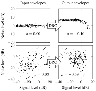
Figure 5: Sample input and output envelope pairs for mixtures of two signals in a DRC system. Top: Speech and white noise. Bottom: Speech and speech.

The ECF models the effects of level-dependent amplification for idealized statistical envelopes, but does not perfectly represent the behavior of real envelope detectors, especially their peak-tracking dynamics. To verify the predicted result under more realistic conditions, an experiment was conducted using mixtures of speech signals from the VCTK database (Veaux et al., 2017) and white Gaussian noise. All signals have the same overall level so that the input SNR is 0 dB. The DRC system has a constant compression ratio of 3:1, that is, a cube-root compression function, in all channels; the filterbank uses 6 Mel-spaced bands from 0 to 8 kHz; and the envelope detector is the filter from Eq. (1) with an attack time of 10 ms and a release time of 50 ms as defined by ANSI S3.22-1996 ($\beta_{\text{a}}=0.978$ and $\beta_{\text{r}}=0.996$ at a sample rate of 16 kHz). The input and output envelope samples were measured using the same envelope detector applied to $s_{1}[t,b]$, $s_{2}[t,b]$, $r_{1}[t,b]$, and $r_{2}[t,b]$.

Figure 5 illustrates the anticorrelation effects of DRC. Each plot shows pairs of envelope samples for two signals in a mixture: the input mixtures $(v_{s_{1}}[t,b],v_{s_{2}}[t,b])$ on the left and the output mixtures $(v_{r_{1}}[t,b],v_{r_{2}}[t,b])$ on the right. The top plots are for speech and white noise and the bottom plots are for two speech signals. The axes have been normalized so that the average input level is 0 dB. The correlation coefficient $\rho$ between samples is computed using the method of Stone and Moore (2007) and averaged across the six channels. The input levels are mostly uncorrelated between the two component signals, but the DRC system shifts the levels according to a vector field similar to that of Fig. 4, producing correlated output points. Because the white noise has nearly constant envelope, the effect of DRC is most apparent at high speech signal levels. When the speech signal is strong, both speech and noise are attenuated, bending the distribution of level pairs downward and producing a negative correlation. The DRC system has a similar effect on the speech mixture; each signal’s level decreases as the level of the other increases, producing a large negative correlation. In an experiment with similar compression parameters but a higher input SNR, Stone and Moore (2008) found an output correlation coefficient of $-0.11$ between speech signals.

It has been shown that the correlation effect is weaker for slower-acting compression, which averages signal levels over hundreds of milliseconds and therefore does not vary gain levels as quickly (Stone and Moore, 2007; Alexander and Masterson, 2015). In a slow-acting compressor, the envelope samples ($v_{s_{1}}[t,b],v_{s_{2}}[t,b]$) are not as widely spread in the $(v_{1},v_{2})$ plane and so they are less distorted by the gain field illustrated in Fig. 4.

5 Effective Compression Performance

The interaction between signals in a DRC system not only introduces distortion to the signal envelopes, it also makes the compressor itself less effective. Intuitively, if a signal of interest is weaker than a noise source, then the noise level will determine the gain applied to both signals and the target signal will not be compressed. Even when the target signal has a higher level, the noise will cause the gain to decrease more slowly than it should with respect to the target level.

To quantify the effect of noise on compression performance, we can measure the change in the output level of the target signal in response to a change in its input level and compare that relationship to the nominal compression ratio. In the hearing literature, it has been observed experimentally that the effective compression ratio of a DRC system is reduced in the presence of noise (Souza et al., 2006). In this section we prove the equivalent result that noise increases the effective compression slope, defined as the log-log slope of the ECF.

Definition 4.

If $\hat{\mathcal{C}}_{b}(v_{1}|v_{2})$ is differentiable with respect to $v_{1}$, then the effective compression slope $\hat{\mathrm{CS}}_{b}(v_{1}|v_{2})$ is given by

$$\hat{\mathrm{CS}}_{b}(v_{1}|v_{2}) =\frac{\partial}{\partial u}\hat{\mathcal{C}}_{b}(e^{u}|v_{2})|_{u=\ln v_{1}}$$ (28)

$$=\frac{\frac{\partial}{\partial v_{1}}\hat{\mathcal{C}}_{b}(v_{1}|v_{2})}{\hat{\mathcal{C}}_{b}(v_{1}|v_{2})}v_{1}.$$ (29)

5.1 Noise reduces compression performance

Using the properties of the ECF, it can be shown that the effective compression slope from Definition 4 is larger than the nominal compression slope from Definition 2—equivalently, the effective compression ratio is smaller than the nominal compression ratio—meaning that in noise the system is less compressive on each component signal than it would be without noise:

$$\boxed{\hat{\mathrm{CS}}_{b}(v_{s_{1}}|v_{s_{2}})\geq\mathrm{CS}_{b}(v_{s_{1}}+v_{s_{2}}),\quad b=1,\dots,B.}$$ (30)

The result follows from the concavity of the ECF.

Theorem 2.

If a compression function $\mathcal{C}(v)$ is differentiable at $v_{x}=v_{1}+v_{2}$, then its effective compression slope satisfies

$$\hat{\mathrm{CS}}(v_{1}|v_{2})\geq\mathrm{CS}(v_{x}),$$ (31)

with equality if $\mathcal{C}(v)$ is linear or if $v_{2}=0$.

Proof.

Because $\mathcal{C}(v)$ is defined to be concave and nonnegative for $v>0$, it follows that

$$\mathcal{C}(v)-v\mathcal{C}^{\prime}(v)\geq 0$$ (32)

for all $v$ at which $\mathcal{C}$ is differentiable, with equality if $\mathcal{C}$ is linear. The effective compression slope is given by

$$\hat{\mathrm{CS}}(v_{1}|v_{2}) =\frac{\frac{\partial}{\partial v_{1}}\hat{\mathcal{C}}(v_{1}|v_{2})}{\hat{\mathcal{C}}(v_{1}|v_{2})}v_{1}$$ (33)

$$=\frac{v_{x}}{\mathcal{C}(v_{x})}\left(\frac{\mathcal{C}^{\prime}(v_{x})v_{1}+\mathcal{C}(v_{x})}{v_{x}}-\frac{\mathcal{C}(v_{x})v_{1}}{v_{x}^{2}}\right)$$ (34)

$$=\frac{\mathcal{C}^{\prime}(v_{x})}{\mathcal{C}(v_{x})}v_{1}+1-\frac{v_{1}}{v_{x}}$$ (35)

$$=\frac{\mathcal{C}^{\prime}(v_{x})}{\mathcal{C}(v_{x})}v_{x}-\frac{\mathcal{C}^{\prime}(v_{x})}{\mathcal{C}(v_{x})}v_{2}+\frac{v_{2}}{v_{x}}$$ (36)

$$=\mathrm{CS}(v_{x})+\frac{v_{2}}{v_{x}\mathcal{C}(v_{x})}(\mathcal{C}(v_{x})-v_{x}\mathcal{C}^{\prime}(v_{x}))$$ (37)

$$\geq\mathrm{CS}(v_{x})$$ (38)

with equality if $\mathcal{C}$ is linear or if $v_{2}=0$. ∎

Equation (37) illustrates that the effective compression slope for a target signal increases with the level of the interfering signal. In fact, in the limit as $v_{s_{1}}/v_{x}$ approaches 0, the effective compression slope approaches 1, so that the system applies linear gain to the target signal. In the low-SNR regime, the gain applied to both signals is determined by the level of the interfering signal. The theorem shows, however, that even at high SNR the compression effect is slightly reduced.

5.2 Experiments

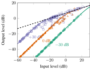
Figure 6: Effective compression function for speech and white noise at different SNRs. The dashed line shows the nominal compression function, the curves show the predicted effective compression functions, and the plotted points show envelope samples measured from the simulated DRC system.

Theorem 2 shows that under an idealized model, additive noise always reduces the effect of compression on a signal of interest. The model, however, does not account for correlations between signals, for the temporal dynamics of the envelope detector, or for peak-tracking effects. To verify this result experimentally, a DRC system was simulated using the same parameters as in the previous section. The signal of interest is a speech recording and the interfering signal is white noise with variable level.

Figure 6 shows the effective compression performance of the system for three signal-to-noise ratios. The dashed line shows the nominal compression function $\mathcal{C}_{b}(v)=v^{1/3}$ for all $b$. The solid curves are the theoretical effective compression functions $\hat{\mathcal{C}}_{b}(v_{s_{1}}|v_{s_{2}})$ for constant noise power $v_{s_{2}}$. The plotted points are samples of the measured input and output envelopes across all channels. Each curve is nearly linear at speech levels much lower than the noise level and closely matches the nominal compression curve at speech levels much higher than the noise level. At high SNR, the speech is compressed correctly, while at low SNR, the gain is determined by the noise level.

These results are consistent with previous work. Souza et al. (2006) measured the effective compression ratio (ECR) empirically using a simulated DRC system and the phase inversion method. The ECR was calculated as the dynamic range of the input envelope divided by the dynamic range of the output envelope, where the dynamic range is defined as the difference between the 95th and 5th percentiles of sample levels in the signals. The ratio was found to increase monotonically with SNR, from 1.06 at $-2$ dB to $1.12$ in quiet for a nominal compression ratio of 2:1. Using the method of Souza et al. (2006) and averaging across signal bands, the ECRs from the experiments here were 1.00 at $-30$ dB SNR, 1.14 at $0$ dB, and 1.69 at $+30$ dB with a nominal compression ratio of 3:1.

6 Signal-to-Noise Ratio

Of the three distortion effects discussed in this work, the impact of DRC on long-term signal-to-noise ratio is both the most studied empirically and the most challenging to analyze mathematically. The levels of the signal components in the output of a compression system depend on the input levels and temporal dynamics of both the signal of interest and the noise. Using the phase inversion method, Souza et al. (2006) found that simulated DRC processing reduced the SNR of a speech signal in speech-shaped noise while linear processing did not. Naylor and Johannesson (2009) observed this effect in commercial hearing aids and showed that it depends on the type of noise, filterbank structure, and envelope time constants. Brons et al. (2015) and Miller et al. (2017) demonstrated the effect in more recent hearing aids that include noise reduction algorithms, which are also nonlinear and can interact with DRC in complex ways (Kortlang et al., 2018). Like the other nonlinear distortion effects described here, SNR reduction appears to be more severe for fast compression (Alexander and Masterson, 2015; May et al., 2018). Reinhart et al. (2017) found that reverberant signals are less affected. Listening tests suggest that fast-acting compression can improve intelligibility with some types of noise but not others, and that these effects depend on the input SNR (Rhebergen et al., 2009, 2017; Kowalewski et al., 2018).

6.1 Signal-to-noise ratio in constant-envelope noise

While it is difficult to say much in general about the effect of compression on SNR, we can prove a result for an important special case: a target signal with a time-varying envelope and a noise signal with constant envelope. Information-rich signals such as speech tend to vary rapidly with time. Many classic speech enhancement algorithms, such as spectral subtraction, rely on the assumption that the noise spectrum is constant while the spectrum of the speech signal varies (Loizou, 2013). At times and frequencies where the input level is large, it is assumed that speech is present and the signal is amplified, while at lower levels the signal is attenuated to remove noise. Because these speech enhancement systems amplify high-level signals and attenuate low-level signals, they act as dynamic range expanders.

If a dynamic range expander can improve SNR, it stands to reason that a compressor might make it worse. To see why, let us analyze the effect of compression on the average SNR over time. Because the envelope is proportional to the power of a signal component, the average SNR at the input is given by

$$\mathrm{SNR}_{\mathrm{in}}[b]=\frac{\mathrm{mean}_{t}v_{s_{1}}[t,b]}{\mathrm{mean}_{t}v_{s_{2}}[t,b]},\quad b=1,\dots,B,$$ (39)

and the average SNR at the output is

$$\mathrm{SNR}_{\mathrm{out}}[b] =\frac{\mathrm{mean}_{t}v_{r_{1}}[t,b]}{\mathrm{mean}_{t}v_{r_{2}}[t,b]}$$ (40)

$$=\frac{\mathrm{mean}_{t}\hat{\mathcal{C}}_{b}(v_{s_{1}}[t,b]|v_{s_{2}}[t,b])}{\mathrm{mean}_{t}\hat{\mathcal{C}}_{b}(v_{s_{2}}[t,b]|v_{s_{1}}[t,b])}.$$ (41)

If the compression function were linear, then the input and output SNRs would be identical. For a concave compression function with convex gain, it can be shown that, if the noise envelope is constant, then the output SNR is lower than the input SNR:

$$\boxed{\mathrm{SNR}_{\mathrm{out}}[b]\leq\mathrm{SNR}_{\mathrm{in}}[b],\quad b=1,\dots,B.}$$ (42)

The proofs in this section rely on an additional technical condition on the compression function. Not only must $\mathcal{C}_{b}(v)$ be nonnegative and concave, the gain function $\mathcal{C}_{b}(v)/v$ must be convex. This condition is satisfied for many smooth compression functions, including linear, power-law, and logarithmic, but not for some functions with corners like that in Fig. 2. This condition ensures that the effective compression function is concave in its first argument and convex in its second.

Lemma 3.

If $\mathcal{C}(v)$ is a compression function and $\mathcal{C}(v)/v$ is convex for all $v>0$, then the effective compression function $\hat{\mathcal{C}}(v_{1}|v_{2})$ is concave in $v_{1}$ and convex in $v_{2}$.

Proof.

See Appendix B. ∎

This property, along with the condition that the interference signal has constant envelope, allows us to prove that the output SNR is no larger than the input SNR.

Theorem 3.

If $\mathcal{C}(v)$ is a compression function and $\mathcal{C}(v)/v$ is convex for all $v>0$, $v_{1}[t]>0$ for all $t$, and $v_{2}[t]=\bar{v}_{2}>0$ for all $t$, then

$$\mathrm{SNR}_{\mathrm{out}}\leq\mathrm{SNR}_{\mathrm{in}}$$ (43)

with equality if $v_{1}[t]$ is constant or $\mathcal{C}$ is linear.

Proof.

Since $v_{2}[t]$ is fixed, the output SNR can be written

$$\mathrm{SNR}_{\mathrm{out}}=\frac{\mathrm{mean}_{t}\hat{\mathcal{C}}(v_{1}[t]|\bar{v}_{2})}{\mathrm{mean}_{t}\hat{\mathcal{C}}(\bar{v}_{2}|v_{1}[t])}.$$ (44)

The numerator is the mean over $t$ of a concave function of $v_{1}[t]$. By Jensen’s inequality (Cover and Thomas, 2006),

$$\mathrm{mean}_{t}\hat{\mathcal{C}}(v_{1}[t]|\bar{v}_{2})\leq\hat{\mathcal{C}}(\mathrm{mean}_{t}v_{1}[t]|\bar{v}_{2}),$$ (45)

with equality when $\mathcal{C}$ is linear or $v_{1}[t]$ is constant. Similarly, the denominator is the mean over $t$ of a convex function of $v_{1}[t]$. Again applying Jensen’s inequality,

$$\mathrm{mean}_{t}\hat{\mathcal{C}}(\bar{v}_{2}|v_{1}[t])\geq\hat{\mathcal{C}}(\bar{v}_{2}|\mathrm{mean}_{t}v_{1}[t]),$$ (46)

with equality when $\mathcal{C}$ is linear or $v_{1}[t]$ is constant. Let $\bar{v}_{1}=\mathrm{mean}_{t}v_{1}[t]$. Since the numerator and denominator of (44) are both positive, we have

$$\mathrm{SNR}_{\mathrm{out}} \leq\frac{\hat{\mathcal{C}}(\bar{v}_{1}|\bar{v}_{2})}{\hat{\mathcal{C}}(\bar{v}_{2}|\bar{v}_{1})}$$ (47)

$$=\frac{\bar{v}_{1}\mathcal{C}(\bar{v}_{1}+\bar{v}_{2})/(\bar{v}_{1}+\bar{v}_{2})}{\bar{v}_{2}\mathcal{C}(\bar{v}_{1}+\bar{v}_{2})/(\bar{v}_{1}+\bar{v}_{2})}$$ (48)

$$=\frac{\bar{v}_{1}}{\bar{v}_{2}}$$ (49)

$$=\mathrm{SNR}_{\mathrm{in}}$$ (50)

with equality when $\mathcal{C}$ is linear or $v_{1}[t]$ is constant. ∎

6.2 Experiments

The equality condition in Theorem 3 suggests that the SNR-reducing effect of compression depends on the curvature of the compression function. Figure 7 compares the input and output SNRs for speech in white noise at different compression ratios. The simulations used a knee-shaped compression function like that in Fig. 2. Although this compressor does not meet the technical condition required for Lemma 3, the results still show the behavior predicted by the theorem. The SNR-reducing effect is greatest at high input SNRs; at low SNRs, the noise level determines the gain and the effective compression function is linear, so the SNR is not affected. Furthermore, higher compression ratios have stronger effects. This phenomenon has been observed in the hearing literature as well: Rhebergen et al. (2009) found similar input-output SNR curves for speech in stationary and interrupted noise (see Fig. 8 of that work). Naylor and Johannesson (2009) obtained similar results using commercial hearing aids configured with different compression ratios (see Fig. 4 of that work).

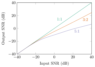
Figure 7: Effect of DRC with different compression ratios on long-term SNR of speech in white noise.

Theorem 3 applies only to constant-envelope noise. While this is an important special case, it does not reflect most real-world sound mixtures. When the target and noise signals both vary with time, the compressor reduces the dynamic range of both signals. The weaker signal will be amplified more and the stronger signal less, pushing their average output levels closer together. Figure 8 shows the results of the SNR experiment with 3:1 knee-shaped compression and different noise types. With white noise, the SNR is always reduced, as predicted by Theorem 3. With speech babble, generated by mixing fourteen VCTK speech clips, the SNR is slightly increased at low input SNRs. When the target and interference signals are both single-talker speech signals, the SNR is improved when it is negative but made worse when it is positive.

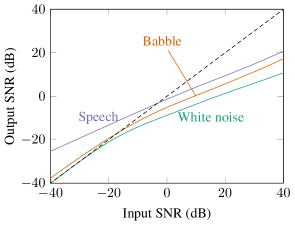
Figure 8: Effect of compression on long-term signal-to-noise ratio of mixtures of speech with different types of noise

These results align well with those observed in the hearing literature. Naylor and Johannesson (2009) found that output SNR is always reduced for speech in unmodulated noise, greatly reduced at positive input SNR and slightly reduced at negative input SNR for speech in modulated noise, and symmetrically increased at negative input SNR and decreased at positive input SNR for a mixture of two speech signals (see Fig. 3 of that work). Reinhart et al. (2017) performed experiments with different numbers of talkers and found a similar symmetric relationship for a mixture of two talkers. The SNR improvement at negative input SNRs declined with each additional interfering talker (see Fig. 3 of that work), consistent with the results for speech babble here.

7 Conclusions

The mathematical analysis above confirms the empirical evidence from the hearing literature that DRC causes distortion in noise. The effects of this distortion depend on the characteristics of the signals, especially their relative levels. The across-source modulation effect is most pronounced at SNRs near unity: when two signals are similar in level, they modulate each other, resulting in a negative correlation between their envelopes. At low SNR, the effective compression function for the target signal becomes nearly linear and the dynamic range of that signal is not changed. Compression algorithms are thus ineffective in challenging listening conditions where they would presumably help most. Meanwhile, at high SNR, the signal of interest is amplified by less than the noise, reducing average SNR.

Can anything be done to improve the performance of DRC systems in noise? The analysis shows that all these effects are caused by the concave curvature of the compression function, which is also what makes the system compressive. It seems, then, that distortion is inevitable whenever signals are compressed as a mixture.

A possible solution is to compress the component signals of a mixture independently, as music producers do when mixing instrumental and vocal recordings. Listening tests have shown improved intelligibility when signals are compressed before rather than after mixing (Stone and Moore, 2008; Rhebergen et al., 2009). Of course, real hearing aids do not have access to the unmixed source signals, so a practical multisource compression system must perform source separation. Hassager et al. (2017) used a single-microphone classification method to separate direct from reverberant signal components, helping to preserve spatial cues that can be distorted by DRC. May et al. (2018) proposed a single-microphone separation system that applies fast-acting compression to speech components and slow-acting compression to noise components; listening experiments with an oracle separation algorithm improved both quality and intelligibility (Kowalewski et al., 2020). Corey and Singer (2017) used a multimicrophone separation method to apply separate compression functions to each of several competing speech signals. The output exhibited better objective measures of across-source modulation distortion, effective compression performance, and SNR compared to a conventional system. It was later shown that larger wearable microphone arrays can provide better multisource compression performance than the small arrays contained in hearing aid earpieces (Corey, 2019).

The mathematical tools introduced in this work can help researchers to understand the distortion effects of conventional DRC systems in noise and to devise new approaches to nonlinear processing for mixtures of multiple signals. The effective compression function models interactions between signal envelopes at the input and output of a DRC system. However, it does not give insights about the effects of the envelope detector or filterbank, which are known to affect the magnitude of all three distortion effects. Further analysis could explain how channel structure and attack and release times affect the distribution of envelope samples.

Like the human auditory system itself, dynamic range compression is a complex nonlinear system that defies simple analysis. By modeling how DRC systems work in the presence of noise, we can design listening systems to help people hear better even in the most challenging environments.

Appendix A Proof of Lemma 2

Lemma 2.

If $f(x)$ is nondecreasing, $g(x)$ is nonincreasing, $X$ is a random variable, and $\mathbb{E}[f(X)]$, $\mathbb{E}[g(X)]$, and $\mathbb{E}[f(X)g(X)]$ exist, then

$$\mathbb{E}\left[f(X)g(X)\right]\leq\mathbb{E}[f(X)]\mathbb{E}[g(X)].$$ (51)

Proof.

Because $f(x)$ is nondecreasing and $g(x)$ is nonincreasing, for every $x$ and $y$ we have

$$\left[f(x)-f(y)\right]\left[g(x)-g(y)\right]\leq 0.$$ (52)

It is sufficient to show that $\mathbb{E}[f(X)g(X)]-\mathbb{E}[f(X)]\mathbb{E}[g(X)]\leq 0$. If $X$ has cumulative distribution function $P(x)$, then

$$\mathbb{E}[f(X)g(X)]-\mathbb{E}[f(X)]\mathbb{E}[g(X)]$$

$$=\int_{x}f(x)g(x)\,\mathrm{d}P(x)-\int_{x}f(x)\,\mathrm{d}P(x)\int_{y}g(y)\,\mathrm{d}P(y)$$ (53)

$$=\int_{x}\int_{y}f(x)[g(x)-g(y)]\,\mathrm{d}P(y)\mathrm{d}P(x)$$ (54)

$$=\int_{x}\int_{y<x}f(x)[g(x)-g(y)]\,\mathrm{d}P(y)\mathrm{d}P(x)$$

$$\quad+\int_{y}\int_{x<y}f(x)[g(x)-g(y)]\,\mathrm{d}P(x)\mathrm{d}P(y)$$ (55)

$$=\int_{x}\int_{y<x}f(x)[g(x)-g(y)]\,\mathrm{d}P(y)\mathrm{d}P(x)$$

$$\quad+\int_{x}\int_{y<x}f(y)[g(y)-g(x)]\,\mathrm{d}P(y)\mathrm{d}P(x)$$ (56)

$$=\int_{x}\int_{y<x}[f(x)-f(y)][g(x)-g(y)]\,\mathrm{d}P(y)\mathrm{d}P(x)$$ (57)

$$\leq 0.$$ (58)

Line (55) swaps the order of integration using Fubini’s theorem (Knapp, 2005) and line (56) exchanges the integration variables $x$ and $y$. ∎

Appendix B Proof of Lemma 3

Lemma 3.

If $\mathcal{C}(v)$ is a compression function and $\mathcal{C}(v)/v$ is convex for all $v>0$, then the effective compression function $\hat{\mathcal{C}}(v_{1}|v_{2})$ is concave in $v_{1}$ and convex in $v_{2}$.

Proof.

Starting with Definition 3 and letting $v_{1}=\lambda p+(1-\lambda)q$,

$$\hat{\mathcal{C}}(v_{1}|v_{2}) =\frac{\mathcal{C}(\lambda p+(1-\lambda)q+v_{2})}{\lambda p+(1-\lambda)q+v_{2}}(\lambda p+(1-\lambda)q)$$ (59)

$$=\mathcal{C}(\lambda(p+v_{2})+(1-\lambda)(q+v_{2}))$$ (60)

$$\quad-v_{2}\frac{\mathcal{C}(\lambda(p+v_{2})+(1-\lambda)(q+v_{2}))}{\lambda(p+v_{2})+(1-\lambda)(q+v_{2})}.$$ (61)

Because $\mathcal{C}(v)$ is concave and $\mathcal{C}(v)/v$ is convex,

$$\hat{\mathcal{C}}(v_{1}|v_{2}) \geq\lambda\mathcal{C}(p+v_{2})+(1-\lambda)\mathcal{C}(q+v_{2})$$ (62)

$$\quad-v_{2}\left(\lambda\frac{\mathcal{C}(p+v_{2})}{p+v_{2}}+(1-\lambda)\frac{\mathcal{C}(q+v_{2})}{q+v_{2}}\right)$$ (63)

$$=\lambda\frac{\mathcal{C}(p+v_{2})}{p+v_{2}}p+(1-\lambda)\frac{\mathcal{C}(q+v_{2})}{q+v_{2}}$$ (64)

$$=\lambda\hat{\mathcal{C}}(p|v_{2})+(1-\lambda)\hat{\mathcal{C}}(q|v_{2}).$$ (65)

Therefore $\hat{\mathcal{C}}(v_{1}|v_{2})$ is concave in $v_{1}$.

Similarly, letting $v_{2}=\lambda p+(1-\lambda)q$,

$$\hat{\mathcal{C}}(v_{1}|v_{2}) =\frac{\mathcal{C}(v_{1}+\lambda p+(1-\lambda)q)}{v_{1}+\lambda p+(1-\lambda)q}v_{1}$$ (66)

$$=\frac{\mathcal{C}(\lambda(v_{1}+p)+(1-\lambda)(v_{1}+q))}{\lambda(v_{1}+p)+(1-\lambda)(v_{1}+q)}v_{1}$$ (67)

$$\leq\lambda\frac{\mathcal{C}(v_{1}+p)}{v_{1}+p}v_{1}+(1-\lambda)\frac{\mathcal{C}(v_{1}+q)}{v_{1}+q}v_{1}$$ (68)

$$=\lambda\hat{\mathcal{C}}(v_{1}|p)+(1-\lambda)\hat{\mathcal{C}}(v_{1}|q).$$ (69)

Therefore $\hat{\mathcal{C}}(v_{1}|v_{2})$ is convex in $v_{2}$. ∎

References

- Alexander and Masterson (2015) Alexander, J. M., and Masterson, K. (2015). “Effects of WDRC release time and number of channels on output SNR and speech recognition,” Ear and Hearing 36(2), e35.
- Alexander and Rallapalli (2017) Alexander, J. M., and Rallapalli, V. (2017). “Acoustic and perceptual effects of amplitude and frequency compression on high-frequency speech,” The Journal of the Acoustical Society of America 142(2), 908–923.
- Allen (2003) Allen, J. B. (2003). “Amplitude compression in hearing aids,” in MIT Encyclopedia of Communication Disorders, edited by R. Kent (MIT Press), pp. 413–423.
- American National Standards Institute (1996) American National Standards Institute (1996). “Specification of hearing aid characteristics (ANSI S3.22-1996)” .
- Brons et al. (2015) Brons, I., Houben, R., and Dreschler, W. A. (2015). “Acoustical and perceptual comparison of noise reduction and compression in hearing aids,” Journal of Speech, Language, and Hearing Research 58(4), 1363–1376.
- Corey (2019) Corey, R. M. (2019). “Microphone array processing for augmented listening,” Ph.D. thesis, University of Illinois at Urbana-Champaign.
- Corey and Singer (2017) Corey, R. M., and Singer, A. C. (2017). “Dynamic range compression for noisy mixtures using source separation and beamforming,” in IEEE Workshop on Applications of Signal Processing to Audio and Acoustics (WASPAA).
- Cover and Thomas (2006) Cover, T. M., and Thomas, J. A. (2006). Elements of Information Theory (Wiley).
- Giannoulis et al. (2012) Giannoulis, D., Massberg, M., and Reiss, J. D. (2012). “Digital dynamic range compressor design—A tutorial and analysis,” Journal of the Audio Engineering Society 60(6), 399–408.
- Hagerman and Olofsson (2004) Hagerman, B., and Olofsson, Å. (2004). “A method to measure the effect of noise reduction algorithms using simultaneous speech and noise,” Acta Acustica United with Acustica 90(2), 356–361.
- Hassager et al. (2017) Hassager, H. G., May, T., Wiinberg, A., and Dau, T. (2017). “Preserving spatial perception in rooms using direct-sound driven dynamic range compression,” The Journal of the Acoustical Society of America 141(6), 4556–4566.
- Jenstad and Souza (2005) Jenstad, L. M., and Souza, P. E. (2005). “Quantifying the effect of compression hearing aid release time on speech acoustics and intelligibility,” Journal of Speech, Language, and Hearing Research 48(3), 651–667.
- Kates (2005) Kates, J. M. (2005). “Principles of digital dynamic-range compression,” Trends in Amplification 9(2), 45–76.
- Kates (2008) Kates, J. M. (2008). Digital Hearing Aids (Plural Publishing).
- Knapp (2005) Knapp, A. W. (2005). Basic Real Analysis (Birkhäuser).
- Kortlang et al. (2018) Kortlang, S., Chen, Z., Gerkmann, T., Kollmeier, B., Hohmann, V., and Ewert, S. D. (2018). “Evaluation of combined dynamic compression and single channel noise reduction for hearing aid applications,” International Journal of Audiology 57, S43–S54.
- Kowalewski et al. (2020) Kowalewski, B., Dau, T., and May, T. (2020). “Perceptual evaluation of signal-to-noise-ratio-aware dynamic range compression in hearing aids,” Trends in Hearing 24, 1–14.
- Kowalewski et al. (2018) Kowalewski, B., Zaar, J., Fereczkowski, M., MacDonald, E. N., Strelcyk, O., May, T., and Dau, T. (2018). “Effects of slow-and fast-acting compression on hearing-impaired listeners’ consonant–vowel identification in interrupted noise,” Trends in Hearing 22, 1–12.
- Loizou (2013) Loizou, P. C. (2013). Speech Enhancement: Theory and Practice (CRC Press).
- Lyon (2017) Lyon, R. F. (2017). Human and machine hearing (Cambridge University Press).
- May et al. (2018) May, T., Kowalewski, B., and Dau, T. (2018). “Signal-to-noise-ratio-aware dynamic range compression in hearing aids,” Trends in Hearing 22, 1–12.
- Miller et al. (2017) Miller, C. W., Bentler, R. A., Wu, Y.-H., Lewis, J., and Tremblay, K. (2017). “Output signal-to-noise ratio and speech perception in noise: effects of algorithm,” International Journal of Audiology 56(8), 568–579.
- Naylor and Johannesson (2009) Naylor, G., and Johannesson, R. B. (2009). “Long-term signal-to-noise ratio at the input and output of amplitude-compression systems,” Journal of the American Academy of Audiology 20(3), 161–171.
- Rallapalli and Alexander (2019) Rallapalli, V. H., and Alexander, J. M. (2019). “Effects of noise and reverberation on speech recognition with variants of a multichannel adaptive dynamic range compression scheme,” International Journal of Audiology 58(10), 661–669.
- Reinhart et al. (2017) Reinhart, P., Zahorik, P., and Souza, P. E. (2017). “Effects of reverberation, background talker number, and compression release time on signal-to-noise ratio,” The Journal of the Acoustical Society of America 142(1), EL130–EL135.
- Rhebergen et al. (2017) Rhebergen, K. S., Maalderink, T. H., and Dreschler, W. A. (2017). “Characterizing speech intelligibility in noise after wide dynamic range compression,” Ear and Hearing 38(2), 194–204.
- Rhebergen et al. (2009) Rhebergen, K. S., Versfeld, N. J., and Dreschler, W. A. (2009). “The dynamic range of speech, compression, and its effect on the speech reception threshold in stationary and interrupted noise,” The Journal of the Acoustical Society of America 126(6), 3236–3245.
- Souza (2002) Souza, P. E. (2002). “Effects of compression on speech acoustics, intelligibility, and sound quality,” Trends in Amplification 6(4), 131–165.
- Souza et al. (2006) Souza, P. E., Jenstad, L. M., and Boike, K. T. (2006). “Measuring the acoustic effects of compression amplification on speech in noise,” The Journal of the Acoustical Society of America 119(1), 41–44.
- Stone and Moore (2004) Stone, M. A., and Moore, B. C. (2004). “Side effects of fast-acting dynamic range compression that affect intelligibility in a competing speech task,” The Journal of the Acoustical Society of America 116(4), 2311–2323.
- Stone and Moore (2007) Stone, M. A., and Moore, B. C. (2007). “Quantifying the effects of fast-acting compression on the envelope of speech,” The Journal of the Acoustical Society of America 121(3), 1654–1664.
- Stone and Moore (2008) Stone, M. A., and Moore, B. C. (2008). “Effects of spectro-temporal modulation changes produced by multi-channel compression on intelligibility in a competing-speech task,” The Journal of the Acoustical Society of America 123(2), 1063–1076.
- Veaux et al. (2017) Veaux, C., Yamagishi, J., and MacDonald, K. (2017). “CSTR VCTK corpus: English multi-speaker corpus for CSTR voice cloning toolkit,” University of Edinburgh. https://doi.org/10.7488/ds/2645.