Common-spectrum process versus cross-correlation for gravitational-wave searches using pulsar timing arrays

Abstract

The North American Nanohertz Observatory for Gravitational Waves (NANOGrav) has recently reported strong statistical evidence for a common-spectrum red-noise process for all pulsars, as seen in their 12.5-yr analysis for an isotropic stochastic gravitational-wave background. However, there is currently very little evidence for quadrupolar spatial correlations across the pulsars in the array, which is needed to make a confident claim of detection of a stochastic background. Here we give a frequentist analysis of a very simple signal+noise model showing that the current lack of evidence for spatial correlations is consistent with the magnitude of the correlation coefficients for pairs of Earth-pulsar baselines in the array, and the fact that pulsar timing arrays are most-likely operating in the intermediate-signal regime. We derive analytic expressions that allow one to compare the expected values of the signal-to-noise ratios for both the common-spectrum and cross-correlation estimators.

I Introduction

A stochastic gravitational-wave background (GWB) is formed from the superposition of GW signals that are either too weak or too numerous to individually detect Maggiore (2000); Christensen (2018). Although we have not yet detected a stochastic background, we know from the advanced LIGO-Virgo detections of individual stellar-mass compact binaries Abbott et al. (2016a, 2017, 2020, 2020) that such a signal exists. So it is just a matter of time before we reach the sensitivity level needed to make a confident detection of the corresponding unresolved GWB signal. For the astrophysical GWB produced by stellar-mass binary black holes (BBHs) throughout the universe, we expect to reach this level by the time the advanced LIGO Aasi et al. (2015) and Virgo Acernese et al. (2015) detectors are operating at design sensitivity (in a couple of years time) Abbott et al. (2016b, 2018). For the analogous GWB produced by supermassive ($\sim\!10^{9}\leavevmode\nobreak\ M_{\odot}$) binary black holes (SMBBHs) associated with galaxy mergers throughout the universe Jaffe and Backer (2003), we may actually be a bit closer to reaching that sensitivity level Rosado et al. (2015); Taylor et al. (2016).

The North American Nanohertz Observatory for Gravitational Waves (NANOGrav) Ransom et al. (2019) has recently reported strong statistical evidence for a common-spectrum red-noise process for all pulsars, as seen in their 12.5-yr analysis for an isotropic stochastic signal Arzoumanian et al. (2020). But there is currently very little evidence for quadrupolar spatial correlations across the pulsars Hellings and Downs (1983), which is needed to make a confident claim of detection of a stochastic gravitational-wave background. As noted in their paper, the current lack of evidence for spatial correlations is consistent with the reduction in signal power that comes from the magnitude of the correlation coefficients for pairs of Earth-pulsar baselines being less than or equal to 0.5. Here we give an explicit proof of that statement in the context of a very simple signal+noise model. Using simple frequentist estimators of the amplitude of the GWB, we show that the common-spectrum (i.e., auto-correlation) estimator has a larger signal-to-noise ratio than a cross-correlation estimator in the intermediate-signal regime Siemens et al. (2013), even if there is no cross-correlated noise to compete against. The estimators that we use have similarities to various frequentist GWB statistics in the pulsar timing literature Anholm et al. (2009); Chamberlin et al. (2015); Rosado et al. (2015), but are purposefully simplified in order to highlight the difference between the auto-correlated and cross-correlated signal.

This simplification of the model leads to a few subtleties in how this model is related to the actual situation. In the simple toy model that we shall describe below, the detection of a red-noise process of any kind would establish the presence of a GWB (in technical terms, the measured signal-to-noise ratio relative to the white-noise-only null hypothesis would be sufficiently greater than zero). But in reality, pulsars have intrinsic red noise that must be distinguished from the common-mode effects of the GWB. While some red noise has long since been clearly detected in many pulsars, an analysis of the properties of the red noise is necessary to detect a common-mode process. We therefore define our signal-to-noise ratios relative to their variance in the presence of a potentially non-zero signal, thus taking into account the variance associated with the GWB itself Rosado et al. (2015). This is in contrast to the optimal statistic Chamberlin et al. (2015), which acts as a detection statistic by defining the noise using the characteristics of a noise-only model. While both of these statistics generically include intrinsic pulsar red noise, we omit this complication for clarity, essentially assuming we have modeled the intrinsic red noise perfectly. The argument of this paper is then that with the same data, in the intermediate-signal regime where modern pulsar timing arrays operate Siemens et al. (2013), one can estimate the amplitude of a GWB using the auto-correlations more precisely than one can estimate it using the cross-correlations. This is essentially what is happening with the NANOGrav 12.5-yr data set, where the auto-correlations can be measured well enough to detect a common-spectrum red-noise process, but the cross-correlations alone cannot yet be measured well enough to provide the unique indication that this is a gravitational-wave signal.

The rest of the paper is organized as follows: In Sec. II, we define our simple signal+noise model, and in Sec. III we calculate the expected signal-to-noise ratios of the amplitude of a potential GWB for the optimal common-spectrum and cross-correlation estimators, in both the weak-signal and intermediate-signal regimes. Our main finding is that the optimal common-spectrum estimator has a larger expected signal-to-noise ratio than the optimal cross-correlation estimator in the intermediate-signal regime, in broad agreement with the results of NANOGrav’s 12.5-yr analysis. We conclude in Sec. IV with a brief discussion, comparing the main results obtained here to expectations for ground-based detectors, and more sophisticated statistical analyses, like those actually performed on the 12.5-yr data Arzoumanian et al. (2020).

II Toy model

We consider a pulsar timing array consisting of $N$ pulsars, with uncorrelated white Gaussian noise described by power spectra

$$P_{n_{a}}(f)=2\sigma_{a}^{2}\,\Delta t\,,\qquad a=1,2,\cdots,N\,,$$ (1)

and a GWB with total auto-correlated power

$$P_{\rm gw}(f)=\frac{A_{\rm gw}^{2}}{12\pi^{2}}\left(\frac{f}{f_{\rm yr}}\right)^{2\alpha}f^{-3},\qquad{\alpha=-2/3}\,,$$ (2)

where $\alpha=-2/3$ is the spectral index appropriate for GW-driven emission from inspiraling SMBBHs Phinney (2001). In the above expressions, $P(f)$ are one-sided power spectral densities for the timing residuals (units of $P(f)$ are ${\rm s}^{2}/{\rm Hz}$); $\sigma_{a}^{2}$ are the noise variances for the pulsars (not necessarily equal to one another); $\Delta t$ is the sampling period (typically one to three weeks for pulsar timing observations); and $f_{\rm yr}\equiv 1/{\rm yr}$ is a reference frequency for evaluating the GWB amplitude.

For simplicity, we will assume that there are only two frequency bins

$$f_{l}\equiv f_{\rm low}\,,\qquad f_{h}\equiv f_{\rm high}\,,$$ (3)

and that the pulsar white noise for all pulsars is much larger than the power in the GWB at high frequencies, so that $P_{n_{a}}(f_{h})\gg P_{\rm gw}(f_{h})$. At low frequencies, the pulsar white noise can be either much greater or much less than the power in the GWB. We call these two regimes the weak-signal and intermediate-signal regimes, respectively Siemens et al. (2013) (Figure 1):

$$P_{\rm gw}(f_{l})\ll P_{n_{a}}(f_{l})\quad\&\quad P_{\rm gw}(f_{h})\ll P_{n_{a}}(f_{h}) ({\rm weak\ signal\ regime})\,,$$ (4)

$$P_{\rm gw}(f_{l})\gg P_{n_{a}}(f_{l})\quad\&\quad P_{\rm gw}(f_{h})\ll P_{n_{a}}(f_{h}) ({\rm intermediate\ signal\ regime})\,.$$ (5)

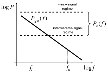
Figure 1: Power spectra for both the GWB and pulsar white noise, allowing for different levels of pulsar noise. For all cases, the pulsar white noise dominates the power in the GWB at high frequencies, $P_{n}(f_{h})\gg P_{\rm gw}(f_{h})$. In the weak-signal regime $P_{\rm gw}(f_{l})\ll P_{n}(f_{l})$, while the intermediate-signal regime has $P_{\rm gw}(f_{l})\gg P_{n}(f_{l})$. For our toy model, we consider only two discrete frequencies $f_{l}$ and $f_{h}$.

The unknown signal and noise parameters are $\sigma_{a}^{2}$ and $A_{\rm gw}^{2}$. But to simplify the analysis, we will work with rescaled parameters $\bar{\sigma}_{a}^{2}$ and $\bar{A}_{\rm gw}^{2}$ so that

$$P_{n_{a}}(f)=\bar{\sigma}_{a}^{2}\,,\quad P_{\rm gw}(f)=\bar{A}{}_{\rm gw}^{2}\,f^{-13/3}\,,\quad a=1,2,\cdots,N\,.$$ (6)

The timing-residual data for the $N$ pulsars can be written in the frequency domain as

$$\tilde{d}_{a}(f)=\tilde{h}_{a}(f)+\tilde{n}_{a}(f)\,,\qquad a=1,2,\cdots,N\,,$$ (7)

where the tildes denote Fourier transforms of the corresponding time-series. The data covariance matrix is given by

$$\tilde{C}(f)=\left(\begin{array}[]{cccc}P_{1}(f)&P_{12}(f)&\cdots&P_{1N}(f)\\ P_{21}(f)&P_{2}(f)&\cdots&P_{2N}(f)\\ \vdots&\vdots&\ddots&\vdots\\ P_{N1}(f)&P_{N2}(f)&\cdots&P_{N}(f)\\ \end{array}\right)\,,$$ (8)

where

$$P_{a}(f)\equiv P_{n_{a}}(f)+P_{\rm gw}(f)\,,\quad P_{ab}(f)=P_{ba}(f)\equiv\chi_{ab}\,P_{\rm gw}(f)\,,$$ (9)

and $\chi_{ab}\equiv\chi(\zeta_{ab})$ is the value of the Hellings-and-Downs correlation function Hellings and Downs (1983) evaluated at the angular separation $\zeta_{ab}$ between two Earth-pulsar baselines (Figure 2).

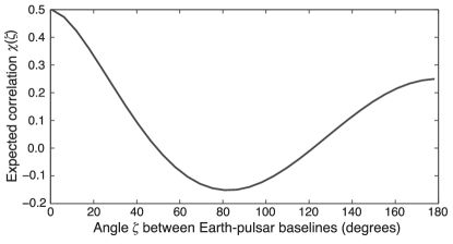
Figure 2: Hellings-and-Downs curve, which gives the expected correlation between the timing residuals measured by two Earth-pulsar baselines as a function of the angle $\zeta$ between the two baselines.

Note that we are assuming here that there is no cross-correlated noise, so that only the GWB power spectrum appears in the off-diagonal terms, multiplied by the Hellings-and-Downs coefficients.

It is also important to emphasize that $P_{\rm gw}(f)$ is the total auto-correlated power induced by the GWB in the timing residuals for each Earth-pulsar baseline. This auto-correlated power has contributions from both the Earth-term and pulsar-term components of the GWB timing-residual response Hellings and Downs (1983), while only the Earth-term components of the response are correlated across pulsars in the array and contribute to $\chi(\zeta)$. This is the reason for the factor of $0.5$ in the normalization of the Hellings-and-Downs curve (Figure 2) at zero angular separation. The total auto-correlated power corresponds to a single Earth-pulsar baseline, while the Hellings-and-Downs curve gives the expected correlation coefficient for two distinct Earth-pulsar baselines, even though the lines-of-sight to the two pulsars might be the same.

The standard estimators for the total auto-correlated and cross-correlated power spectra are

$$\hat{P}_{a}(f)\equiv\frac{2}{T}|\tilde{d}_{a}(f)|^{2}\,,\qquad\hat{P}_{ab}(f)\equiv\frac{2}{T}{\rm Re}[\tilde{d}_{a}(f)\tilde{d}_{b}^{*}(f)]\,,$$ (10)

where $T$ is the total observation time, and the factor of 2 has been included to make these one-sided power spectrum estimates. Since we only have two frequencies to work with, we have $2N$ complex data points

$$\tilde{d}_{al}\equiv\tilde{d}_{a}(f_{l})\,,\quad\tilde{d}_{ah}\equiv\tilde{d}_{a}(f_{h})\,,\qquad a=1,2,\cdots,N\,,$$ (11)

from which to construct estimators for the $N+1$ parameters $\bar{\sigma}_{a}^{2}$ and $\bar{A}_{\rm gw}^{2}$.

Given the inequalities in (5), it immediately follows that the white noise variances $\bar{\sigma}_{a}^{2}$, can be estimated simply from the high-frequency estimators of the auto-correlated power:

$$\hat{\bar{\sigma}}_{a}^{2}\equiv\hat{P}_{a}(f_{h})=\frac{2}{T}|\tilde{d}_{ah}|^{2}\,,\qquad a=1,2,\cdots,N\,.$$ (12)

Similarly, the amplitude $\bar{A}_{\rm gw}^{2}$ of the power in the GWB can be estimated from either the difference between the auto-correlated power at low frequency and the white noise estimators at high frequency:

$$\hat{A}_{a}^{2}\,f_{l}^{-13/3}\equiv\hat{P}_{a}(f_{l})-\hat{\bar{\sigma}}^{2}_{a}=\frac{2}{T}\left(|\tilde{d}_{al}|^{2}-|\tilde{d}_{ah})|^{2}\right)\,,\qquad a=1,2,\cdots,N\,,$$ (13)

or the cross-correlated power at low frequencies

$$\hat{A}_{ab}^{2}\,f_{l}^{-13/3}\equiv{\hat{P}_{ab}(f_{l})}/{\chi_{ab}}=\frac{2}{T}{{\rm Re}[\tilde{d}_{al}\tilde{d}_{bl}^{*}]}/{\chi_{ab}}\,,\qquad ab=12,13,\cdots\,,$$ (14)

where the number of distinct pulsar pairs $ab$ is given by $N_{\rm pairs}\equiv N(N-1)/2$. (We do not consider cross-correlation estimators evaluated at high frequencies, since the power in the GWB at high frequencies is less than that at low frequencies by a large factor, $(f_{h}/f_{l})^{13/3}$.) We will call the estimators $\hat{A}_{a}^{2}$, which are constructed from the auto-correlated power spectrum estimates, common-spectrum or common-process estimators. Similarly, we will call the estimators $\hat{A}_{ab}^{2}$, which are constructed from the cross-correlated power spectrum estimates, cross-correlation or Hellings-and-Downs estimators. Note that in all cases, the expectation value of these estimators (averaged over different signal and noise realizations) is just the amplitude of the power in the GWB:

$$\langle\hat{A}_{a}^{2}\rangle=\langle\hat{A}_{ab}^{2}\rangle=\bar{A}_{\rm gw}^{2}\,.$$ (15)

We can further construct optimal (i.e., minimal-variance, unbiased) estimators of $\bar{A}_{\rm gw}^{2}$ by forming appropriate linear combinations of these individual estimators. Since we are interested in this paper in comparing the common-spectrum and cross-correlation estimators, we will define and analyze these two estimators separately in the following section.

III Optimal estimators

To construct optimal linear combinations of the individual common-spectrum and cross-correlation estimators defined in the previous section, we need to calculate the covariance matrices of these estimators, from which we obtain the optimal weighting factors. This is a consequence of a general result, which says that given $N$ estimators $\hat{X}_{i}$ of some quantity $X$, the optimal linear combination of the $\hat{X}_{i}$ is given by the weighted average

$$\hat{X}_{\rm opt}\equiv\frac{\sum_{i}\lambda_{i}\hat{X}_{i}}{\sum_{j}\lambda_{j}}\,,\qquad\lambda_{i}\equiv\sum_{j}\left(C^{-1}\right)_{ij}\,,$$ (16)

where $C_{ij}$ are the components of the covariance matrix for the estimators:

$$C_{ij}\equiv\langle\hat{X}_{i}\hat{X}_{j}\rangle-\langle\hat{X}_{i}\rangle\langle\hat{X}_{j}\rangle\,.$$ (17)

It is easy to show that the expected value of $\hat{X}_{\rm opt}$ is $X$ (since $\langle\hat{X}_{i}\rangle=X$ and $X_{\rm opt}$ is normalized), and that its variance is given by

$$\sigma^{2}_{\rm opt}\equiv\langle\hat{X}_{\rm opt}^{2}\rangle-\langle\hat{X}_{\rm opt}\rangle^{2}=\frac{1}{\sum_{i}\lambda_{i}}=\frac{1}{\sum_{i,j}\left(C^{-1}\right)_{ij}}\,.$$ (18)

Proof: The second equality in the above expression for $\sigma_{\rm opt}^{2}$ follows from

$$\left(\sum\lambda\right)^{-2}\sum_{i,j}\lambda_{i}\lambda_{j}\langle\hat{X}_{i}\hat{X}_{j}\rangle-X^{2} =\left(\sum\lambda\right)^{-2}\sum_{i,j}\lambda_{i}\lambda_{j}(C_{ij}+\langle\hat{X}_{i}\rangle\langle\hat{X}_{j}\rangle)-X^{2}$$ (19)

$$=\left(\sum\lambda\right)^{-2}\sum_{i,j}\sum_{k,l}(C^{-1})_{ik}(C^{-1})_{jl}C_{ij}$$

$$=\left(\sum\lambda\right)^{-2}\sum_{k,l}(C^{-1})_{kl}=\left({\sum\lambda}\right)^{-1}\,.$$

The square of the expected signal-to-noise ratio of the optimal estimator is thus

$$\rho^{2}_{\rm opt}\equiv\frac{\langle\hat{X}_{\rm opt}\rangle^{2}}{\sigma_{\rm opt}^{2}}=X^{2}\,\sum_{i,j}\left(C^{-1}\right)_{ij}\,.$$ (20)

The above construction is a generalization of standard $1/\sigma_{i}^{2}$ inverse-noise weighting of $N$ independent estimators $\hat{X}_{i}$, which allows for correlations between the estimators.

III.1 Optimal common-spectrum estimator

The optimal linear combination of the common-spectrum estimators $\hat{A}_{a}^{2}$, where $a=1,2,\cdots,N$, is thus given by

$$\hat{A}_{\rm CP}^{2}\equiv\frac{\sum_{a}\lambda_{a}\hat{A}_{a}^{2}}{\sum_{b}\lambda_{b}}\,,\qquad\lambda_{a}\equiv\sum_{b}\left(C^{-1}\right)_{ab}\,,$$ (21)

where the subscript ‘CP’ stands for common process, and $C_{ab}$ are the components of the $N\times N$ covariance matrix

$$C_{ab}\equiv\langle\hat{A}_{a}^{2}\hat{A}_{b}^{2}\rangle-\langle\hat{A}_{a}^{2}\rangle\langle\hat{A}_{b}^{2}\rangle\,.$$ (22)

To calculate the components $C_{ab}$ of the covariance matrix, we will need to evaluate expectation values of the form

$$\langle|\tilde{d}_{al}|^{2}|\tilde{d}_{bl}|^{2}\rangle\,,\quad\langle|\tilde{d}_{ah}|^{2}|\tilde{d}_{bh}|^{2}\rangle\,,\quad\langle|\tilde{d}_{al}|^{2}|\tilde{d}_{bh}|^{2}\rangle\,,\quad\langle|\tilde{d}_{ah}|^{2}|\tilde{d}_{bl}|^{2}\rangle\,,$$ (23)

where $a=b$ for the diagonal elements. To do so, we will make use of the following identity for zero-mean Gaussian random variables:

$$\langle XYZW\rangle=\langle XY\rangle\langle ZW\rangle+\langle XZ\rangle\langle YW\rangle+\langle XW\rangle\langle YZ\rangle\,.$$ (24)

We will also use the following expressions for the various quadratic expectation values:

$$\langle\tilde{d}_{a}(f)\tilde{d}_{b}^{*}(f)\rangle=\frac{T}{2}\,P_{ab}(f)\,,$$ (25)

$$\langle\tilde{d}_{a}(f)\tilde{d}_{b}^{*}(f^{\prime})\rangle=0\ {\rm if}\ f\neq f^{\prime}\,,$$ (26)

$$\langle\tilde{d}_{a}(f)\tilde{d}_{b}(f)\rangle=\langle\tilde{d}_{a}(f)\tilde{d}_{b}^{*}(-f)\rangle=0\ {\rm if}\ f\neq 0\,,$$ (27)

$$\langle\tilde{d}_{a}^{*}(f)\tilde{d}_{b}^{*}(f)\rangle=\langle\tilde{d}_{a}(-f)\tilde{d}_{b}^{*}(f)\rangle=0\ {\rm if}\ f\neq 0\,.$$ (28)

Note that the last two results hold even if $a=b$.

Using the above results, we find

$$C_{aa}=f_{l}^{26/3}\left(P_{\rm gw}^{2}(f_{l})+2\bar{\sigma}_{a}^{2}P_{a}(f_{l})\right)\,,\qquad C_{ab}=\left(\bar{A}_{\rm gw}^{2}\right)^{2}\chi_{ab}^{2}\,.$$ (29)

for the diagonal and off-diagonal elements of the covariance matrix for the common-spectrum estimators. These expressions simplify in the weak-signal and intermediate-signal regimes. In these limits

$$C_{ab}\simeq 2f_{l}^{26/3}(\bar{\sigma}_{a}^{2})^{2}\,\delta_{ab} ({\rm weak\ signal\ regime})\,,$$ (30)

$$C_{ab}\simeq(\bar{A}_{\rm gw}^{2})^{2}\chi_{ab}^{2} ({\rm intermediate\ signal\ regime})\,,$$ (31)

where $\chi_{ab}=1$ in the last expression if $a=b$. Note that in the weak-signal regime, the covariance matrix is diagonal, which means that the individual common-spectrum estimators are independent of one another. In contrast, in the intermediate-signal regime, the covariance matrix has non-negligible off-diagonal terms corresponding to covariances between the estimators, which reduces the number of independent terms in the weighted average.

Using (20), we can now calculate the square of the expected signal-to-noise ratio for the optimal combination of common-spectrum estimators in these two limits. We just need to invert the above covariance matrices and sum their components. To simplify the calculation further we will assume that the pulsar white noise power $\bar{\sigma}_{a}^{2}$ is the same for all pulsars—i.e., $\bar{\sigma}_{a}^{2}\equiv\bar{\sigma}^{2}$. Then for the $N=45$ pulsars used in NANOGrav’s 12.5-year analysis, we find

$$\rho^{2}_{\rm CP}\simeq\frac{45}{2}P_{\rm gw}^{2}(f_{l})/(\bar{\sigma}^{2})^{2} ({\rm weak\ signal\ regime})\,,$$ (32)

$$\rho^{2}_{\rm CP}\simeq 20.0 ({\rm intermediate\ signal\ regime})\,.$$ (33)

Note that the factor of $45/2$ in the first expression comes from $(C^{-1})_{ab}$ being proportional to the identity matrix $\delta_{ab}$ in the weak-signal regime with $\bar{\sigma}_{a}^{2}=\bar{\sigma}^{2}$ for all pulsars. This is reduced slightly to 20 in the intermediate-signal regime, due to the off-diagonal terms in the inverse covariance matrix.

III.2 Optimal Hellings-and-Downs estimator

We now perform a similar calculation for the Hellings and Downs cross-correlation estimators $\hat{A}^{2}_{ab}$, where $ab=12,13,\cdots$. To evaluate the components $C_{ab,cd}$ of the $N_{\rm pairs}\times N_{\rm pairs}$ covariance matrix between these estimators, we need to evaluate expectation values of the form

$$\langle\tilde{d}_{al}\tilde{d}_{bl}^{*}\tilde{d}_{cl}\tilde{d}_{dl}^{*}\rangle\,,\quad\langle\tilde{d}_{al}^{*}\tilde{d}_{bl}\tilde{d}_{cl}\tilde{d}_{dl}^{*}\rangle\,,\quad\langle\tilde{d}_{al}\tilde{d}_{bl}^{*}\tilde{d}_{cl}^{*}\tilde{d}_{dl}\rangle\,,\quad\langle\tilde{d}_{al}^{*}\tilde{d}_{bl}\tilde{d}_{cl}^{*}\tilde{d}_{dl}\rangle\,,$$ (34)

where $a\neq b$, $c\neq d$, but one or two pulsars might be shared between the pairs $ab$ and $cd$. (For example, the diagonal elements of the covariance matrix have $c=a$ and $d=b$.) There are thus three cases to consider, and which lead to the following results:

1. when $ab$ and $cd$ do not share any pulsar in common:

   $$C_{ab,cd}=\frac{1}{2}(\bar{A}_{\rm gw}^{2})^{2}\,\left(\frac{\chi_{ac}\chi_{bd}+\chi_{ad}\chi_{bc}}{\chi_{ab}\chi_{cd}}\right)\,,$$ (35)

2. when $ab$ and $cd$ share one pulsar in common, e.g., $c=a$:

   $$C_{ab,ad}=\frac{1}{2}(\bar{A}_{\rm gw}^{2})^{2}\,\left(1+\frac{P_{a}(f_{l})}{P_{\rm gw}(f_{l})}\frac{\chi_{bd}}{\chi_{ab}\chi_{ad}}\right)\,,$$ (36)

3. when $ab$ and $cd$ share two pulsars in common, e.g., $c=a$, $d=b$:

   $$C_{ab,ab}=\frac{1}{2}(\bar{A}_{\rm gw}^{2})^{2}\,\left(1+\frac{P_{a}(f_{l})P_{b}(f_{l})}{P_{\rm gw}^{2}(f_{l})}\frac{1}{\chi_{ab}^{2}}\right)\,.$$ (37)

These expressions simplify in the weak-signal and intermediate-signal regimes to

$$C_{ab,cd}\simeq 0\,,\qquad C_{ab,ad}\simeq 0\,,\qquad C_{ab,ab}\simeq\frac{1}{2}f_{l}^{26/3}\,{\bar{\sigma}_{a}^{2}\bar{\sigma}_{b}^{2}}/{\chi_{ab}^{2}}\,\qquad({\rm weak\ signal\ regime})\,,$$ (38)

and

$$\left.\begin{array}[]{l}C_{ab,cd}\simeq\frac{1}{2}\left(\bar{A}_{\rm gw}^{2}\right)^{2}\,\left(\frac{\chi_{ac}\chi_{bd}+\chi_{ad}\chi_{bc}}{\chi_{ab}\chi_{cd}}\right)\\ C_{ab,ad}\simeq\frac{1}{2}\left(\bar{A}_{\rm gw}^{2}\right)^{2}\,\left(1+\frac{\chi_{bd}}{\chi_{ab}\chi_{ad}}\right)\\ C_{ab,ab}\simeq\frac{1}{2}\left(\bar{A}_{\rm gw}^{2}\right)^{2}\,\left(1+\frac{1}{\chi_{ab}^{2}}\right)\end{array}\quad\right\}\qquad({\rm intermediate\ signal\ regime})\,.$$ (39)

Just as we did for the optimal common-spectrum estimator, we can calculate the square of the expected signal-to-noise ratio of the optimal Hellings-and-Downs estimator in these two limits by appropriately summing the elements of the inverse covariance matrix, $(C^{-1})_{ab,cd}$. Assuming as before that $\bar{\sigma}_{a}^{2}=\bar{\sigma}^{2}$ for all pulsars, we find

$$\rho^{2}_{\rm HD}\simeq 2\sum_{ab}\chi_{ab}^{2}\,{P_{\rm gw}^{2}(f_{l})}/{(\bar{\sigma}^{2})^{2}}\approx 66\,{P_{\rm gw}^{2}(f_{l})}/{(\bar{\sigma}^{2})^{2}} ({\rm weak\ signal\ regime})\,,$$ (40)

$$\rho^{2}_{\rm HD}\simeq 4.66 ({\rm intermediate\ signal\ regime})\,,$$ (41)

for the $N=45$ pulsars used in NANOGrav’s 12.5-yr analysis. Note the drastic reduction from 66 to 4.66 in the expressions for the squared signal-to-noise ratio in the weak-signal and intermediate-signal regimes. This is due to the presence of non-negligible off-diagonal terms in the inverse covariance matrix for the intermediate-signal regime, which reduces the number of independent terms in the weighted average.

III.3 Comparison

It is now a simple matter to compare the expected signal-to-noise ratios for the optimal common-spectrum and Hellings-and-Downs estimators. Using the results in (32), (33), (40), (41), we find

$${\rho_{\rm CP}}/{\rho_{\rm HD}}\approx 0.6 ({\rm weak\ signal\ regime})\,,$$ (42)

$${\rho_{\rm CP}}/{\rho_{\rm HD}}\approx 2.1 ({\rm intermediate\ signal\ regime})\,.$$ (43)

Note that this last result, as well as the values for the individual signal-to-noise ratios in the intermediate-signal regime ($\rho_{\rm CP}\approx 4.5$ and $\rho_{\rm HD}\approx 2.2$) are broadly consistent with NANOGrav’s recent analysis Arzoumanian et al. (2020) of their 12.5-yr data, where they found much stronger evidence for a common-spectrum process than for Hellings-and-Downs cross correlations.

We see that the transition between the weak-signal and intermediate-signal regimes leads to a reversal of the signal-to-noise preference between using the optimal common-spectrum estimator or Hellings-and-Downs cross-correlation estimator. In the weak-signal regime, the noise is dominated by white noise, and the fact that there are more pairs of pulsars than individual pulsars means that there is more averaging available for the cross-correlation estimator than the common-spectrum (i.e., auto-correlation) estimator. In the intermediate-signal regime, the variance of the GWB itself dominates, and because the Earth-term component of the signal is correlated across the sky, the number of independent terms in the average is considerably less than the number of pairs of pulsars, and the benefit of averaging is reduced by roughly an order of magnitude. The common-spectrum estimator also suffers a reduction in the number of independent measurements in the intermediate-signal regime, but this effect is relatively smaller since the pulsar-term component of the signal is uncorrelated and the number of auto-correlations is smaller. As a result, once the variance of the GWB itself dominates, as is the case in the NANOGrav 12.5-yr data, the signal-to-noise balance begins to favor the auto-correlations. Figure 3 illustrates the transition between the weak-signal and intermediate-signal regimes, using the full expressions for the covariance matrices (29) and (35), (36), (37) to calculate the expected signal-to-noise ratios $\rho_{\rm CP}$ and $\rho_{\rm HD}$. This calculation is done for the $N=45$ NANOGrav 12.5-yr pulsars.

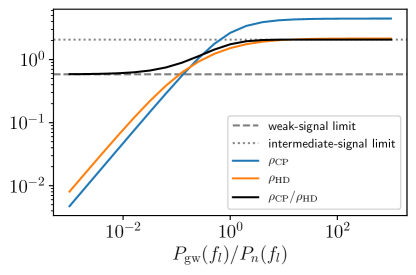
Figure 3: Reversal of signal-to-noise preference from $\rho_{\rm HD}$ to $\rho_{\rm CP}$ as one transitions from the weak-signal regime to the intermediate-signal regime. The ratios given in (42) and (43) are represented here by the dashed and dotted horizontal lines. This figure is for the $N=45$ NANOGrav 12.5-yr pulsars.

IV Discussion

We conclude this paper with a couple of remarks:

(i) The main result—that NANOGrav should see evidence of a GWB first in the auto-correlations and then in the cross-correlations—is specific to pulsar timing analyses and is not expected for ground-based detectors like advanced LIGO and Virgo. This is because the advanced LIGO and Virgo detectors are operating in the weak-signal regime, where $P_{\rm gw}(f)\ll P_{n}(f)$ for all frequencies. Hence, for LIGO-Virgo analyses, it is most efficacious to look for evidence of a GWB in the cross-correlations Allen and Romano (1999); Romano and Cornish (2017), where there is little Thrane et al. (2013, 2014); Coughlin et al. (2016, 2018); Meyers et al. (2020) or no cross-correlated noise to compete against. In contrast, pulsar timing arrays are most-likely currently operating in the intermediate-signal regime Siemens et al. (2013), where the power in the GWB dominates that of the noise at low frequencies. As the total observation time increases, one has access to lower frequencies (since $f_{\rm min}\sim 1/T$), where the power in a GWB with a steep red-noise spectral index (e.g., $-13/3$ for SMBBH inspirals) can more easily exceed the pulsar noise power (assuming the noise is white or less red than the GWB), and move us into the intermediate-signal regime. For ground-based detectors, increasing the total observation time does not allow one to access frequencies below $\sim 10\leavevmode\nobreak\ {\rm Hz}$, which are dominated by seismic and gravity-gradient noise.

(ii) As mentioned above, the analyses presented in Secs. II and III uses simple frequentist estimators and their expected signal-to-noise ratios to compare the relative likelihood of seeing a GWB in the auto-correlations versus the cross-correlations. This approach was chosen for its relative simplicity as opposed to its statistical rigor. A more proper analysis would begin by writing down the likelihood functions for the various signal+noise models being considered—i.e., (i) noise only, (ii) noise plus a GWB that is present only via the auto-correlation terms, and (iii) noise plus a GWB that is present in both the auto-correlation and cross-correlation terms, with the correlation coefficients given by the values of the Hellings and Downs curve (Figure 2). One would then compare these different signal+noise models via maximum-likelihood ratios or Bayes factors, to see which model is preferred by the data. But since these are the types of analyses that were actually performed by NANOGrav when analyzing their 12.5-yr data Arzoumanian et al. (2020), we did not think that it would be particularly illuminating to rederive those statistics here. Rather, we thought that a “back-of-the-envelope” illustration that a GWB signal will first appear as a common-spectrum process would have value to somebody outside the field.

References

- Maggiore (2000) M. Maggiore, “Gravitational wave experiments and early universe cosmology,” Phys. Rep. 331, 283–367 (2000), gr-qc/9909001 .
- Christensen (2018) Nelson Christensen, “Stochastic gravitational wave backgrounds,” Reports on Progress in Physics 82, 016903 (2018).
- Abbott et al. (2016a) B. P. Abbott et al. (LIGO Scientific Collaboration and Virgo Collaboration), “Observation of Gravitational Waves from a Binary Black Hole Merger,” Phys. Rev. Lett. 116, 061102 (2016a).
- Abbott et al. (2017) B. P. Abbott et al. (LIGO Scientific Collaboration and Virgo Collaboration), “GW170817: Observation of Gravitational Waves from a Binary Neutron Star Inspiral,” Phys. Rev. Lett. 119, 161101 (2017).
- Abbott et al. (2020) R. Abbott et al., “GWTC-2: Compact Binary Coalescences Observed by LIGO and Virgo During the First Half of the Third Observing Run,” (2020), arXiv:2010.14527 [gr-qc] .
- Aasi et al. (2015) J. Aasi et al. (LIGO Scientific), “Advanced LIGO,” Class. Quant. Grav. 32, 074001 (2015), arXiv:1411.4547 [gr-qc] .
- Acernese et al. (2015) F. Acernese et al. (Virgo), “Advanced Virgo: a second-generation interferometric gravitational wave detector,” Class. Quant. Grav. 32, 024001 (2015), arXiv:1408.3978 [gr-qc] .
- Abbott et al. (2016b) B. P. Abbott et al. (LIGO Scientific Collaboration and Virgo Collaboration), “GW150914: Implications for the Stochastic Gravitational-Wave Background from Binary Black Holes,” Phys. Rev. Lett. 116, 131102 (2016b).
- Abbott et al. (2018) B. P. Abbott et al. (LIGO Scientific Collaboration and Virgo Collaboration), “GW170817: Implications for the Stochastic Gravitational-Wave Background from Compact Binary Coalescences,” Phys. Rev. Lett. 120, 091101 (2018).
- Jaffe and Backer (2003) A. H. Jaffe and D. C. Backer, “Gravitational Waves Probe the Coalescence Rate of Massive Black Hole Binaries,” Astrophysical Journal 583, 616–631 (2003), arXiv:astro-ph/0210148 .
- Rosado et al. (2015) P. A. Rosado, A. Sesana, and J. Gair, “Expected properties of the first gravitational wave signal detected with pulsar timing arrays,” MNRAS 451, 2417–2433 (2015), arXiv:1503.04803 [astro-ph.HE] .
- Taylor et al. (2016) S. R. Taylor, M. Vallisneri, J. A. Ellis, C. M. F. Mingarelli, T. J. W. Lazio, and R. van Haasteren, “Are We There Yet? Time to Detection of Nanohertz Gravitational Waves Based on Pulsar-timing Array Limits,” ApJ 819, L6 (2016), arXiv:1511.05564 [astro-ph.IM] .
- Ransom et al. (2019) Scott Ransom, A. Brazier, S. Chatterjee, T. Cohen, J. M. Cordes, M. E. DeCesar, P. B. Demorest, J. S. Hazboun, M. T. Lam, R. S. Lynch, M. A. McLaughlin, S. M. Ransom, X. Siemens, S. R. Taylor, and S. J. Vigeland, “The NANOGrav Program for Gravitational Waves and Fundamental Physics,” in BAAS, Vol. 51 (2019) p. 195, arXiv:1908.05356 [astro-ph.IM] .
- Arzoumanian et al. (2020) Zaven Arzoumanian, Paul T. Baker, Harsha Blumer, Bence Becsy, Adam Brazier, Paul R. Brook, Sarah Burke-Spolaor, Shami Chatterjee, Siyuan Chen, James M. Cordes, Neil J. Cornish, Fronefield Crawford, H. Thankful Cromartie, Megan E. DeCesar, Paul B. Demorest, Timothy Dolch, Justin A. Ellis, Elizabeth C. Ferrara, William Fiore, Emmanuel Fonseca, Nathan Garver-Daniels, Peter A. Gentile, Deborah C. Good, Jeffrey S. Hazboun, A. Miguel Holgado, Kristina Islo, Ross J. Jennings, Megan L. Jones, Andrew R. Kaiser, David L. Kaplan, Luke Zoltan Kelley, Joey Shapiro Key, Nima Laal, Michael T. Lam, T. Joseph W. Lazio, Duncan R. Lorimer, Jing Luo, Ryan S. Lynch, Dustin R. Madison, Maura A. McLaughlin, Chiara M. F. Mingarelli, Cherry Ng, David J. Nice, Timothy T. Pennucci, Nihan S. Pol, Scott M. Ransom, Paul S. Ray, Brent J. Shapiro-Albert, Xavier Siemens, Joseph Simon, Renee Spiewak, Ingrid H. Stairs, Daniel R. Stinebring, Kevin Stovall, Jerry P. Sun, Joseph K. Swiggum, Stephen R. Taylor, Jacob E. Turner, Michele Vallisneri, Sarah J. Vigeland, and Caitlin A. Witt, “The NANOGrav 12.5-year Data Set: Search For An Isotropic Stochastic Gravitational-Wave Background,” (2020), arXiv:2009.04496 [astro-ph.HE] .
- Hellings and Downs (1983) R. W. Hellings and G. S. Downs, “Upper limits on the isotropic gravitational radiation background from pulsar timing analysis,” 265, L39–L42 (1983).
- Siemens et al. (2013) Xavier Siemens, Justin Ellis, Fredrick Jenet, and Joseph D Romano, “The stochastic background: scaling laws and time to detection for pulsar timing arrays,” Classical and Quantum Gravity 30, 224015 (2013).
- Anholm et al. (2009) M. Anholm, S. Ballmer, J. D. E. Creighton, L. R. Price, and X. Siemens, “Optimal strategies for gravitational wave stochastic background searches in pulsar timing data,” Phys. Rev. D 79, 084030 (2009), arXiv:0809.0701 [gr-qc] .
- Chamberlin et al. (2015) S. J. Chamberlin, J. D. E. Creighton, X. Siemens, P. Demorest, J. Ellis, L. R. Price, and J. D. Romano, “Time-domain implementation of the optimal cross-correlation statistic for stochastic gravitational-wave background searches in pulsar timing data,” Phys. Rev. D 91, 044048 (2015), arXiv:1410.8256 [astro-ph.IM] .
- Phinney (2001) E. S. Phinney, “A Practical Theorem on Gravitational Wave Backgrounds,” ArXiv Astrophysics e-prints (2001), astro-ph/0108028 .
- Allen and Romano (1999) Bruce Allen and Joseph D. Romano, “Detecting a stochastic background of gravitational radiation: Signal processing strategies and sensitivities,” Physical Review D 59, 102001 (1999), arXiv:gr-qc/9710117 [gr-qc] .
- Romano and Cornish (2017) Joseph D. Romano and Neil. J. Cornish, “Detection methods for stochastic gravitational-wave backgrounds: a unified treatment,” Living Reviews in Relativity 20, 2 (2017), arXiv:1608.06889 [gr-qc] .
- Thrane et al. (2013) Eric Thrane, Nelson Christensen, and Robert Schofield, “Correlated magnetic noise in global networks of gravitational-wave interferometers: observations and implications,” Phys. Rev. D87, 123009 (2013), arXiv:1303.2613 [astro-ph.IM] .
- Thrane et al. (2014) E. Thrane, N. Christensen, R. M. S. Schofield, and A. Effler, “Correlated noise in networks of gravitational-wave detectors: subtraction and mitigation,” Phys. Rev. D90, 023013 (2014), arXiv:1406.2367 [astro-ph.IM] .
- Coughlin et al. (2016) Michael W. Coughlin et al., “Subtraction of correlated noise in global networks of gravitational-wave interferometers,” Class. Quant. Grav. 33, 224003 (2016), arXiv:1606.01011 [gr-qc] .
- Coughlin et al. (2018) Michael W. Coughlin et al., “Measurement and subtraction of Schumann resonances at gravitational-wave interferometers,” Phys. Rev. D97, 102007 (2018), arXiv:1802.00885 [gr-qc] .
- Meyers et al. (2020) Patrick M. Meyers, Katarina Martinovic, Nelson Christensen, and Mairi Sakellariadou, “Detecting a stochastic gravitational-wave background in the presence of correlated magnetic noise,” (2020), arXiv:2008.00789 [gr-qc] .
- Hazboun et al. (2019) Jeffrey S. Hazboun, Joseph D. Romano, and Tristan L. Smith, “Realistic sensitivity curves for pulsar timing arrays,” Phys. Rev. D 100, 104028 (2019), arXiv:1907.04341 [gr-qc] .
- Blandford et al. (1984) R. Blandford, R. Narayan, and R. W. Romani, “Arrival-time analysis for a millisecond pulsar.” Journal of Astrophysics and Astronomy 5, 369–388 (1984).