Revenue Maximization and Learning in Product Ranking

We consider the revenue maximization problem for an online retailer who plans to display in order a set of products differing in their prices and qualities. Consumers have attention spans, i.e., the maximum number of products they are willing to view, and inspect the products sequentially before purchasing a product or leaving the platform empty-handed when the attention span gets exhausted. Our framework extends the well-known cascade model in two directions: the consumers have random attention spans instead of fixed ones and the firm maximizes revenues instead of clicking probabilities. We show a nested structure of the optimal product ranking as a function of the attention span when the attention span is fixed. Using this fact, we develop an approximation algorithm when only the distribution of the attention spans is given. Under mild conditions, it achieves $1/e$ of the revenue of the clairvoyant case when the realized attention span is known. We also show that no algorithms can achieve more than 0.5 of the revenue of the same benchmark. The model and the algorithm can be generalized to the ranking problem when consumers make multiple purchases. When the conditional purchase probabilities are not known and may depend on consumer and product features, we devise an online learning algorithm that achieves $\tilde{\mathcal{O}}(\sqrt{T})$ regret relative to the approximation algorithm, despite the censoring of information: the attention span of a customer who purchases an item is not observable. Numerical experiments demonstrate the outstanding performance of the approximation and online learning algorithms.

Ningyuan Chen
Rotman School of Management, University of Toronto, ningyuan.chen@utoronto.ca
Anran Li
Department of Management, London School of Economics and Political Science, a.li26@lse.ac.uk
Shuoguang Yang
Department of Industrial Engineering and Decision Analytics, HKUST, yangsg@ust.hk,

1 Introduction

Online retailing has seen steady growth over the last decade. According to the Digital Commerce analysis of the US Commerce Department’s year-end retail data, online sales constituted 16% of all retail sales in 2019 and reached higher levels due to the impact of COVID-19. For an e-commerce platform, one of the most important decisions is the products’ display positioning as it plays a crucial role in shaping customers’ shopping behavior. Empirical evidence abounds. Baye et al. (2009) find that a consumer’s likelihood of purchasing from a firm is strongly related to the order in which the firm is listed on a webpage by a search engine. In the online advertising industry, it has been widely observed that ads placed higher on a webpage attract more clicks from consumers (Agarwal et al. 2011, Ghose and Yang 2009). So the products displayed at the top positions can naturally enjoy higher exposure and therefore higher revenue. Given the importance of product ranking positions, the key question for online platform is how to rank the products to maximize the total revenue.

To answer the question, it is crucial to characterize and quantify how exactly customers react to products ranked in different positions. As one of the most popular behavioral models for product ranking, the cascade model has proved its salience and robustness in extensive experimental studies. In the cascade model, a customer with a reserved utility threshold sequentially views the displayed products from top to bottom. Had the customer viewed an item ranked in a certain position, if the product provides a net utility higher than her threshold, then the customer purchases the product and leaves right away. Otherwise, the customer moves on to view the product ranked in the next position. The model succinctly captures the one-way substitutability top-ranked products impose on bottom-ranked products. rev:no-satisficingIn a large experimental study, Craswell et al. (2008) find that the cascade model best explains the consumer behavior among a number of competing hypotheses. In particular, the customer views products sequentially and directly proceeds to purchase a product once the utility of the product exceeds an acceptable threshold, skipping the remaining products. The empirical success and theoretical tractability have made the cascade model the most widely used model in the literature (see, e.g., Kempe and Mahdian 2008).

However, the cascade model doesn’t provide a sufficient explanation to why a large fraction of customers may leave without purchasing a product. Indeed, the cascade model is originally motivated by clicks on search results, in which leaving without clicking on anything is rare. As a result, when using the cascade model for product ranking, “leaving” only occurs when a satisfactory product has been found or all products have been exhausted. In contrast, eye-tracking experiments show that consumers are more likely to examine the items near the top of the list and may leave without purchasing any product before reaching the bottom of the page (Feng et al. 2007). This phenomenon can be explained by the limited attention span of customers: if a customer arrives with an intrinsic attention span $n$, then she may leave after viewing at most $n$ products regardless of whether a purchase has been made. According to Feng et al. (2007), consumers’ attention to an item decreases exponentially with its distance to the top, indicating that the distribution of attention span decays rapidly.

In this paper, we introduce random attention spans to the cascade model. In our model, the attention span of a customer determines the maximum number of items she is willing to view. We capture the limited attention by assigning each customer an attention span sampled from a distribution. When a customer arrives, she sequentially views the displayed products decided by the e-commerce platform (also referred to as the “firm” or the “retailer”) according to the cascade model. Once the attention span is reached or a satisfactory product is found, the customer leaves the firm. Thus, in our model, customers leave for two reasons. First, she may purchase a product in the display whose utility exceeds the threshold for the first time and leave, even though there could be another product with a higher utility within the rest of her attention span. Second, a customer may have exhausted her attention before finding anything satisfactory, in which case she leaves without buying anything or viewing more products.

Within the model, we study the firm’s optimal display order of products in order to maximize the potential revenue. When some of the information is unknown, such as the distribution of the attention span and the attractiveness of the products, we propose a learning algorithm that extracts the information from past observations and maximizes revenues simultaneously. Our contribution is threefold.

• We incorporate attention spans and revenue maximization into the well-known cascade model. rev:cascadeIn the literature on cascade models, the objective of the firm is typically to maximize the purchase rate of customers, which renders the optimal ranking decision trivial. Indeed, the firm only needs to rank the products in the descending order of their attractiveness. To maximize the revenue, however, the prices of the products also have to be considered. When the attention span is fixed, we develop a dynamic programming algorithm to find the optimal ranking leveraging the fact that the products displayed at the bottom would not cannibalize the demand from the top. We show a surprising nested structure of the optimal ranking and the marginal revenue decreases as the attention span increases. That is, for customers of attention span $x$, the optimal ranking of $x$ products is a subset of that for customers with attention span $x+1$, although the additional product could be inserted in any position under optimality. We also provide sufficient and necessary conditions when the optimal ranking is a prefix as the attention span increases, which is a stronger structure than the nested.

• Despite the structure of the optimal ranking under fixed attention spans, the computational cost can still be prohibitively high when the attention span is random. We develop a novel approximation algorithm for ranking optimization. It leverages the concavity of the optimal revenue as the attention span increases, thanks to the nested structure of the optimal ranking. When the random attention spans have an increasing failure rate (IFR), an assumption satisfied by many distributions, the resulting revenue ratio is $1/e$ relative to a clairvoyant who can access the realized attention span of each customer. We show that no ranking can achieve a revenue higher than 1/2 of the same clairvoyant. So the optimality gap of our algorithm is at most $1/2-1/e\approx 0.13.$ We also look at special cases, for example, when the optimal ranking is a prefix as the attention span increases or when the attention span is geometrically distributed, under which we can provide polynomial-time optimal algorithms. More interestingly, we show that the model and the algorithm can be generalized to the ranking optimization problem when consumers make multiple purchases in a single visit.

• When the customers’ behavior is not known a priori, including the distribution of the attention spans and the attractiveness of the products, the firm may have to learn the unknown information and maximize the revenue simultaneously. What makes the problem challenging is the presence of consumer features and product features, two defining characteristics of online retailing. We consider the interaction (outer product) between both features that determines the product attractiveness. In addition, when customers leave the firm after making a purchase, the attention span information is censored. We propose an online learning algorithm by constructing unbiased estimators for the distribution of the attention span and combining them with the UCB approach to learn the product attractiveness. It achieves good performance ($\tilde{\mathcal{O}}(\sqrt{T})$ regret) relative to the offline algorithm.

2 Literature Review

There are two streams of literature that are closely related to this study: (1) choice models (especially those taking the positions of products into account) and the corresponding optimal assortment planning, (2) the online learning of product ranking models. We review the two streams separately below.

2.1 Consumer Choice Models and Assortment Optimization

Most classic discrete choice models do not take the positions of products into account. The assortment optimization problem determines the optimal subset of products to include in the assortment to maximize the revenue. For example, Mahajan and van Ryzin (2001), Talluri and Van Ryzin (2004) show that under the well-known multinomial logit (MNL) model, the optimal assortment includes the products with the highest prices. Since this paper studies product ranking, the optimization involves the display order of products. It is significantly different from this line of literature in terms of models and algorithms.

rev:literature-rankingRecently, there have been a number of studies focusing on the business case when consumers may inspect products sequentially or based on their display positions, which is more relevant in online retailing. Next we compare our paper with these studies from the angles of model setups and results. Abeliuk et al. (2016) incorporate the position bias into the deterministic utilities of the MNL model. Their model describes the choice behavior in the population but does not provide a sequential choice model for individual customers. In Gallego et al. (2020), a customer arrives with a random attention span (similar to our model). She then chooses the preferred product among all the products in the span according to a choice model. This is in contrast to our model in which customers choose products sequentially and do not recall past products. Therefore, the optimal assortment in Gallego et al. (2020) does not exhibit the nested property (Theorem 4.3). The model in Aouad and Segev (2020) is similar to Gallego et al. (2020), but focuses on the MNL choice model. In Derakhshan et al. (2022), the customers search products sequentially. They first form their consideration set using an optimal stopping problem to maximize the expected surplus (due to the existence of search cost) and then choose the product inside the consideration set using the MNL model. This model doesn’t consider attention spans and focuses on the maximization of market share instead of revenues. In Chen et al. (2020), the authors model this problem using mechanism design when the sellers of the products have private information. A few recent papers extend discrete choice models to multiple stages. Flores et al. (2019), Feldman and Segev (2019), Liu et al. (2020), Gao et al. (2021) extend the MNL model to multiple stages. In each stage, the customer chooses a product based on the MNL model and leaves the market if a product is chosen; otherwise, the customer moves on to the next stage. The optimization problem is usually NP-hard and the authors give approximation methods. Although the model in this study can be treated as a special case of the models studied in these papers when each stage only has one product, there are two important differences. First, random attention spans are not considered in these papers. Second, we are able to derive richer structures and constant-bound approximation algorithms specific to our setting. Recently, Brubach et al. (2022) study a similar problem in the online matching framework. They design an approximate algorithm using linear programming that obtains $1/2$-approximation relative to the LP upper bound. They also show that any algorithm can be arbitrarily bad relative to the clairvoyant that foresees the realized attention span. Our focus is on the nested structure of the optimal ranking for fixed attention spans, which allows us to drive a different approximation algorithm that achieves $1/e$-approximation relative to the clairvoyant instead of the LP upper bound under the mild IFR assumption of attention span distribution. Moreover, our algorithm can be generalized to the purchase of multiple products (Section C in the Appendix), which has not been studied in the display optimization literature. In fact, our model can be viewed as a generalization of the well-known cascade model in Kempe and Mahdian (2008), which provides a quasi-polynomial-time approximation scheme (QPTAS) with a $(\frac{1}{4}-\epsilon)$-approximation guarantee. We study the revenue maximization of the cascade model with random attention spans and derive structural properties of the optimal ranking. This setup and derived results are novel in the literature on cascade models. From the perspective of algorithmic design, the approximation algorithm proposed in this study is primarily inspired by the nested structure (Theorem 4.3). This structure and algorithm are not known in the papers mentioned above.

The random attention span considered in this study is analogous to similar behavioral setups in the literature. The primary motivation is the cognitive cost for customers to view and evaluate a large number of products in online retailing. Wang and Sahin (2018) build a model where the customers first form a consideration set by weighing between their expected utility and the search effort. The products in the consideration set are then thoroughly evaluated. Gallego and Li (2017) study the operational decisions of a model with random consideration sets where customers have a fixed preference order and each product enters the consideration set with an exogenous probability. Aouad et al. (2019) relax the fixed preference order assumption of the random consideration set model and focus on an assortment setting.

2.2 Online Learning

The multi-armed bandit framework has seen great success in modeling the exploration/exploitation trade-off for many applications. See Bubeck and Cesa-Bianchi (2012) for a comprehensive survey. In particular, in the field of revenue management, there have been many studies on demand learning and price experimentation using this framework, since the early seminal works by Araman and Caldentey (2009), Besbes and Zeevi (2009), Broder and Rusmevichientong (2012). Many extensions and new features have been studied, such as network revenue management (Besbes and Zeevi 2012, Ferreira et al. 2018, Chen et al. 2019), personalized dynamic pricing (Chen and Gallego 2020, 2018, Miao et al. 2019, Ban and Keskin 2020), limited price experimentations (Cheung et al. 2017), and non-stationarity (Besbes et al. 2015). Readers may refer to den Boer (2015) for a review of papers in this area.

There are several papers applying the multi-armed bandit framework to assortment planning, such as Rusmevichientong et al. (2010), Sauré and Zeevi (2013). Agrawal et al. (2019) consider the learning problem in the well-known MNL choice model under general assumptions compared to the literature. Their algorithm simultaneously explores the optimal assortment and attempts to maximize the revenue. Kallus and Udell (2020) investigate a similar problem under the contextual setting, when customers of different types have various preferences. They exploit the low-rank nature of the parameters to design efficient algorithms. In a related paper, Chen et al. (2018) assume that the contextual information can be non-stationary over time. Oh and Iyengar (2019) leverage Thompson sampling to learn the optimal assortment in the MNL model. The methods used in the literature cannot be directly applied to our model, because customers have dramatically different behavior in a product ranking model from the MNL model. Therefore, our algorithm differs in what to learn and how to actively experiment.

Our work is closely related to the papers studying the learning of the cascade model and product ranking models. The first such algorithm, called “cascading bandits”, is proposed in Kveton et al. (2015). It learns the optimal set of items to display in order to maximize the click rate, when the firm can observe the clicking behavior of past customers. Due to the wide range of applications in online advertising and recommendation systems of the cascade model, the online learning algorithm for such models under generic settings and contextual information has been extensively studied by Katariya et al. (2016), Zoghi et al. (2017), Lagrée et al. (2016), Kveton et al. (2015) and Zong et al. (2016), Cheung et al. (2019).

Compared to cascading bandits, our work has three major differences in problem formulations, which require novel treatments when designing algorithms. First, the items in the cascade model are only differentiated by their clicking probabilities. In our setting, the items generate different revenues. Second, the customers in the cascade model never abandon the system early, while in our model, they have a random attention span whose distribution needs to be learned. These two changes make our problem much more challenging. In the cascade model, the offline optimal solution is rather straightforward: finding the set of items with the highest clicking rates. In our model, it is not clear how to solve the offline problem exactly. Indeed, Kempe and Mahdian (2008) study a similar problem, and are only able to provide a $(1/4-\epsilon)$-approximation algorithm. Third, when a customer purchases an item and leaves the system before reaching the limit of the attention span, this information is censored to the firm. We develop novel unbiased estimators to handle the censored observations.

Recently, the learning of product ranking models that generalize the cascade model has drawn attention in the Operations Research community. Ferreira et al. (2022) study a model in which the attention span and the clicking probabilities can be correlated. In this dimension, their model is more general than ours. They focus on maximizing the probability that a customer clicks at least one item. As a result, a greedy policy that ranks products sequentially is $1/2$-optimal. The greedy policy is their learning target, whose structure can be exploited. In contrast, because we focus on revenue maximization, the target policy doesn’t have a structure to facilitate learning. Golrezaei et al. (2021) propose an algorithm that learns the optimal ranking in the presence of fake users. Gao et al. (2022) investigate the optimal pricing of the cascade model, in which the clicking and purchasing probabilities are parametrized and need to be learned. Their model is more structured and the nested structure doesn’t seem to hold in their model. Their major focus is on pricing and the design of the algorithm deviates significantly from ours. Niazadeh et al. (2020) consider the online learning problem of Asadpour et al. (2020) and focus on the maximization of the sum of a sequence of submodular functions, subject to a permutation of the inputs. It is closely connected to product ranking. However, because we focus on revenue maximization instead of clicking rates, the objective function is no longer submodular. A recent paper (Zhang, Ahn, and Baardman 2022) consider the joint problem of inventory and ranking under a click-then-convert model. The online learning portion of our model is similar to Cao and Sun (2019), Cao et al. (2019). The major distinction is our focus on maximizing the revenue instead of clicks. As mentioned above, the difference in the objective leads to completely different offline optimal solutions. Therefore, the resulting learning algorithm and the analysis differ.

3 The Model

Let $[n]\triangleq\{1,\ldots,n\}$ denote the universal set of products. There is an online retailer (he) who chooses an assortment $S\subset[n]$ to display and rank them in order within $M$ slots. We use $\sigma\in P(S)$ to refer to a permutation $\sigma$ of $S$, where $P(S)$ is the set of all permutations of items in $S$. More precisely, for $i\in\left\{1,\dots,|S|\right\}$, we use $\sigma(i)\in S$ to denote the product displayed in the $i$-th position. Equivalently, for a product $j\in S$, the firm displays it in the $\sigma^{-1}(j)$-th position.

When a consumer (she) arrives, she views the products sequentially. However, the retailer cannot perfectly predict how many products she is willing to view. Therefore, we capture it by a random attention span $X$, with distribution $g_{x}\triangleq\Pr(X=x)$ and tail probability denoted by $G_{x}\triangleq\Pr(X\geq x)$ for $x=1,2,\dots$. For a consumer with attention span $x$ drawn from $X$, she views product $\sigma(1)$ first and purchases it if it is satisfactory, i.e., the utility exceeds the no-purchase option. If she purchases the first product, then she leaves and the firm garners revenue $r_{\sigma(1)}$. Otherwise, she moves on to the second product and repeats the process until she finds a product satisfactory or has viewed $x$ products, after which she leaves permanently. We assume that the probability of product $j$ being satisfactory is independent of everything else and denote it by $\lambda_{j}$, i.e., conditional on viewing product $j$, the probability that she would purchase it. For the rest of the paper, we refer to it as conditional purchase probability. The consumer keeps viewing the products till she finds one satisfactory or exhausts her attention span $x$, at which point she leaves without purchasing anything.

Therefore, each product $j\in[n]$ is associated with a conditional purchase probability $\lambda_{j}$ and price $r_{j}$. Both quantities are assumed to be fixed and known in the offline setting. (In Section 5, we consider the case when $\lambda_{j}$ is unknown and to be learned, which may depend on customer/product features.) We index the products such that

$$r_{1}\geq r_{2}\geq\dots\geq r_{n};\quad\lambda_{j}>\lambda_{j+1}\ \text{if}\ r_{j}=r_{j+1}.$$ (1)

In other words, the products are indexed in the descending order of their prices and then in the descending order of their conditional purchase probabilities if the prices are equal. We assume no products have identical characteristics (the combination of price and conditional purchase probability).

Given that position $k$ is within a consumer’s attention span, her purchase probability of product $\sigma(k)$ is

$$\prod_{i=1}^{k-1}(1-\lambda_{\sigma(i)})\cdot\lambda_{\sigma(k)}.$$

In other words, the consumer purchases product $\sigma(k)$ if it is satisfactory while all products displayed earlier are not. $1-\lambda_{\sigma(i)}$ is the cannibalization effect that a product at position $i$ exerts on the products displayed later.

3.1 Revenue Maximization for the Retailer

The firm’s goal is to choose an assortment $S$ of at most $M$ products, as well as its ranking $\sigma\in P(S)$, in order to maximize the expected revenue garnered from a potential consumer. From the earlier introduction we see that the expected revenue from a consumer with an attention span $x$ can be expressed as

$$R(\sigma,x)\triangleq\sum_{k=1}^{x\wedge M}\prod_{i=1}^{k-1}(1-\lambda_{\sigma(i)})\cdot\lambda_{\sigma(k)}r_{\sigma(k)}.$$ (2)

When a customer arrives, as the retailer does not know her attention span, he takes the expected value of $x\sim X$ in (2) and obtains the total expected revenue

$$\mathbb{E}[R(\sigma,X)]= \sum_{x=1}^{M}g_{x}R(\sigma,x)=\sum_{x=1}^{M}g_{x}\Big{(}\sum_{k=1}^{x}\prod_{i=1}^{k-1}(1-\lambda_{\sigma(i)})\cdot\lambda_{\sigma(k)}r_{\sigma(k)}\Big{)}$$

$$= \sum_{x=1}^{M}\prod_{i=1}^{x-1}(1-\lambda_{\sigma(i)})\cdot\lambda_{\sigma(x)}r_{\sigma(x)}G_{x}.$$ (3)

Therefore, the optimization problem for the firm is the joint assortment, i.e., choosing an $S\subset N$ such that $|S|\leq M$, and ranking, i.e., deciding $\sigma\in P(S)$ to maximize the total expected revenue from a random customer:

$$\max_{S\subset N,\sigma\in P(S)}\,\mathbb{E}[R(\sigma,X)].$$ (4)

From (2) we can see that a product displayed at a later slot does not cannibalize the demand and therefore the revenue for the earlier. As a result, the optimal ranking would occupy all the $M$ slots and we only focus on assortments such that $|S|=M$.

Note that one customer purchasing at most one product is a defining feature of discrete choice models. And for the cascade model, it is also primarily motivated by clicking one relevant item from online searches. Although the single item clicking/purchasing is widely adopted in the literature, the assumption may be limiting in online retailing: for example, a customer may add several products to the cart on Amazon before checking out. In Section C in the Appendix, by relaxing the cannibalization factor to a broader range, we extend the model to capture multiple purchases. That is, a customer may continue viewing and selecting the products after making some purchases. We show that most results derived in the next section still hold in that setting. In this sense, our work is more general than any of the current discrete choice model based display optimization literature.

Note that if $r_{j}\equiv 1$ for all $j\in[n]$, then our model encompasses the well-known classic cascade model (Craswell et al. 2008) as a special case. In this case, the online retailer tries to maximize the click rate, or equivalently, the purchasing probability of at least one product. For the cascade model, the optimal solution follows an intuitive structure: ranking the products in the descending order of their conditional purchase probabilities $\lambda_{j}$. In the general case when $r_{j}$’s are not identical, the products are differentiated along two dimensions, and it is unclear how to trade off between their conditional purchase probabilities and prices. For example, it is natural to rank a product with high conditional purchase probability and high price in the top position. However, in most practical scenarios, a product with higher conditional purchase probability is often associated with a lower price. Should the firm first display products that are more attractive or more profitable? How does the decision depend on the display capacity $M$ and the distribution of attention spans? We present the following example to shed some light on the complexity of these questions.

Example 3.1

Suppose the online retailer is selling three products, with revenues and conditional purchase probability $(r_{j},\lambda_{j})$ as: $(1,1)$, $(9,0.1)$ and $(1.9,0.52)$. The capacity is $M=2$. When the customer only views one product ($X\equiv 1$), the optimal ranking is to display product one, which has the highest conditional purchase probability, in the first position. So an optimal ranking is $\sigma^{1}=\{1\}$ and $R(\sigma^{1},1)=1$.

Now suppose the customer always views two products ($X\equiv 2$). As the customer is willing to view more positions, the retailer would prefer to place a product with higher profit first, though it may have a lower conditional purchase probability. So an optimal ranking is $\sigma^{2}=\{2,1\}$ and $R(\sigma^{2},2)=1.8$.

Next consider the case when the attention span is random. When $\Pr(X=1)=0.9$ and $\Pr(X=2)=0.1$, it can be shown that the optimal ranking $\sigma^{*}$ is neither $\sigma^{1}$ nor $\sigma^{2}$. In fact, we have $\mathbb{E}[R(\sigma^{1},X)]=R(\sigma^{1},1)=1$ and $\mathbb{E}[R(\sigma^{2},X)]=0.9\cdot 9\cdot 0.1+0.1\cdot R(\sigma^{2},2)=0.99$. On the other hand, one can show that $\sigma^{*}=\{3,1\}$ generates $\mathbb{E}[R(\sigma^{*},X)]=0.9\cdot 1.9\cdot 0.52+0.1\cdot(1.9\cdot 0.52+0.48\cdot 1\cdot 1)=1.036$. Surprisingly, product three never appears in the optimal rankings for fixed attention spans, but should be placed on the top when the attention span is random.    

Example 3.1 demonstrates the intricacy of the optimal ranking for random attention spans. A natural question, then, is whether the optimal ranking can be efficiently solved. It turns out that this is a notoriously difficult problem: It shares a similar formulation to the Slate Cascade Model in Kempe and Mahdian (2008), which claims that it is an open question to show the NP-hardness and provides a quasi-polynomial-time approximation scheme (QPTAS) with $(1/4-\epsilon)$-approximation guarantee. We devote the next section to a new approximation algorithm that improves the approximation ratio to $1/e$ under a wide class of distributions of $X$.

4 Best-x Algorithm for Optimal Ranking

With the complexity of the problem, we focus on developing a fast and easy-to-implement approximation algorithm for (4) and show there is a performance bound of the garnered revenue. Before presenting our approximation algorithm, we first investigate the revenue maximization problem when the attention span is fixed. It turns out that the problem has rich structures, based on which we then develop an approximation algorithm for random spans.

4.1 Revenue Maximization for Fixed Attention Spans

Suppose the retailer is expecting a customer with fixed attention span $x\leq M$. Recall that $M$ is the number of available slots so for $x>M$ we can truncate it to $x=M$. To maximize the revenue, the retailer would choose an assortment of size $|S|=x$. We first provide a lemma characterizing the optimal ranking when the assortment $S$ is given.

Lemma 4.1

Fix attention span at $x$. Suppose the assortment $S$ with size $|S|=x$ is given and $\sigma^{x}$ maximizes $R(\sigma,x)$ among $\sigma\in P(S)$. We have that the products in $\sigma^{x}$ are displayed in increasing order of their product indices, i.e., $\sigma^{x}(i)\leq\sigma^{x}(i+1)$ for $i=1,\dots,|S|-1$.

Combined with condition (1), Lemma 4.1 implies that the products in the optimal ranking are displayed in the descending order of their prices and then in the descending order of their conditional purchase probabilities if there are ties in prices. Lemma 4.1 looks counter-intuitive at the first sight as it prioritizes the price over the conditional purchase probability. rev:expensive-firstTo understand the intuition, note that we focus on a customer with a fixed attention span $x$, i.e., she would always view $x$ products or purchase the first satisfactory product. Given an assortment and ranking, by swapping expensive products to the top, the customer would view expensive products first, which increases the expected revenue.

Although Lemma 4.1 reduces the problem of finding the optimal ranking under a fixed attention span to finding the optimal assortment, it is still a daunting task. Namely, the number of assortments with given size $M$ is exponential in $M$. It is computationally intractable to compare the expected revenues of all possible assortments/rankings and pick the optimal one. However, in light of Lemma 4.1, we can develop a dynamic program to quickly solve the joint assortment/ranking problem. The dynamic program employs both the optimal ranking result from Lemma 4.1 and the fact that the revenue $R(\sigma,x)$ can be computed recursively, i.e.,

$$R(\sigma,x) \triangleq\sum_{k=1}^{x}\prod_{i=1}^{k-1}(1-\lambda_{\sigma(i)})\cdot\lambda_{\sigma(k)}r_{\sigma(k)}$$

$$=\lambda_{\sigma(1)}r_{\sigma(1)}+(1-\lambda_{\sigma(1)})\big{(}\sum_{k=2}^{x}\prod_{i=2}^{k-1}(1-\lambda_{\sigma(i)})\cdot\lambda_{\sigma(k)}r_{\sigma(k)}\big{)}$$

$$=\lambda_{\sigma(1)}r_{\sigma(1)}+(1-\lambda_{\sigma(1)})R(\sigma[2,x],x-1)$$ (5)

$$=R(\sigma[2,x],x-1)+\lambda_{\sigma(1)}\big{(}r_{\sigma(1)}-R(\sigma[2,x],x-1)\big{)},$$

where we use $\sigma[2,x]$ to denote the sub-ranking of $\sigma$ from $2$ to $x$. Note that $R(\sigma[2,x],x-1)$ is the revenue from the display $\sigma[2,x]$ when the consumer has attention span $x-1$. Intuitively, had we known the top position displays product $j$, then the optimal sub-ranking $\sigma[2,x]$ should be chosen from the set $\{j+1,j+2,\dots,n\}$ to maximize $R(\sigma[2,x],x-1)$ by (5). This is because according to Lemma 4.1, the indices of the rest of the products should not be smaller than $j$. This structure inspires Algorithm 1. In the algorithm, $H_{j}^{x}$ and $\sigma_{j}^{x}$ stand for the optimal revenue and ranking for customers with attention span $x$, when the products are chosen from $\{j,j+1,\dots,n\}$.

Algorithm 1 Assortment Optimization Given $X=x$

0:  $r_{j}$, $\lambda_{j}$ for $j\in[n]$, $x$

  $H^{0}_{j}=0$ for all $j=1,2,\dots,n$; $H^{k}_{n+1}=0$ for all $k=0,1,2,\dots,x$; $\sigma^{0}_{j}=\emptyset$ for all $j=1,2,\dots,n$; $\sigma^{k}_{n+1}=\emptyset$ for all $k=0,1,2,\dots,x$

  for $k=1,\ldots,x$  do

     for $j=n,\ldots,1$  do

        

$$H^{k}_{j}\leftarrow\max\Big{\{}H^{k-1}_{j+1}+\lambda_{j}\big{(}r_{j}-H^{k-1}_{j+1}\big{)},\,H^{k}_{j+1}\Big{\}}$$ (6)

        if $\Big{(}H^{k-1}_{j+1}+\lambda_{j}\big{(}r_{j}-H^{k-1}_{j+1}\big{)}\Big{)}\geq H^{k}_{j+1}$ then

           $\quad\sigma^{k}_{j}\leftarrow\sigma^{k-1}_{j+1}\cup\{j\}$

        else

           $\quad\sigma^{k}_{j}\leftarrow\sigma^{k}_{j+1}$

        end if

     end for

  end for

  return  $H^{x}_{1}$ and $\sigma^{x}_{1}$

With a slight abuse of notations, when $\sigma^{k}_{j}$ is optimized to be $\sigma^{k-1}_{j+1}\cup\{j\}$, Lemma 4.1 uniquely determines its ranking order.

Although there might be multiple optimal rankings, Algorithm 1 always outputs one with a specific property. In particular, for two rankings $|\sigma|=|\sigma^{\prime}|=x$, we say $\sigma$ is lexicographically less than $\sigma^{\prime}$ if for all $i=1,\dots,x$, $\sigma(i)\leq\sigma^{\prime}(i)$. The next result shows that Algorithm 1 always finds the optimal ranking with the least lexicographic value (referred to as the $\mathcal{L}$-optimal ranking) for attention span $x$, denoted as $\sigma^{x}$.

Proposition 4.2

For a customer with fixed attention span $x$, Algorithm 1 returns the $\mathcal{L}$-optimal ranking.

The property of $\mathcal{L}$-optimal rankings plays an important role in the analysis. Two rankings $\sigma$ and $\sigma^{\prime}$ are said to have a nested structure, or, $\sigma\subset\sigma^{\prime}$, if for all $i\in\sigma$ there exists an $i^{\prime}\in\sigma^{\prime}$ such that $\sigma(i)=\sigma^{\prime}(i^{\prime})$ and for all $i,\,i^{\prime}=1,\dots,|\sigma|-1$, if $\sigma(i)<\sigma(i^{\prime})$, then $\sigma^{\prime}(i)<\sigma^{\prime}(i^{\prime})$. In other words, $\sigma\subset\sigma^{\prime}$ if the assortment of $\sigma$ is a subset of that of $\sigma^{\prime}$ and the products are ranked in the same order.

The next proposition demonstrates a nested structure for the $\mathcal{L}$-optimal rankings as the customer’s fixed attention span increases.

Proposition 4.3

The $\mathcal{L}$-optimal rankings have a nested structure:

$$\sigma^{1}\subset\sigma^{2}\subset\dots\subset\sigma^{M}.$$ (7)

Proposition 4.3 states that the optimal ranking for customers of attention span $x+1$ can be obtained by inserting or appending one product to the optimal ranking for attention span $x$. For example, suppose there are 5 products and the $\mathcal{L}$-optimal ranking for $x=3$ is $\sigma^{3}=\{1,3,4\}$. Then the $\mathcal{L}$-optimal ranking for $x=4$ might be $\sigma^{4}=\{1,2,3,4\}$ or $\sigma^{4}=\{1,3,4,5\}$.

Proposition 4.3 naturally leads to a simple algorithm to compute $\sigma^{x}$ for all $x\in[M]$. In particular, Algorithm 2 provides an iterative approach to compute the $\mathcal{L}$-optimal assortment. Note that we only need to find the optimal assortment, and the ranking is automatically determined by Lemma 4.1.

Algorithm 2 Assortment Optimization for Fixed Attention Spans (AssortOpt)

0:  $r_{j}$, $\lambda_{j}$ for $j\in[n]$

   $\sigma^{0}\leftarrow\emptyset$

  for $x=1,\dots,M$  do

     Update $\sigma^{x}\leftarrow\argmax_{\sigma=\sigma^{x-1}\cup\{j\}}R(\sigma,x)$

  end for

  return  $\{\sigma^{x}\}_{x=1}^{M}$

Based on Proposition 4.3, we are able to show the following structural property, which serves as a building block for the approximation algorithm. In particular, we can show that the marginal revenue from increasing the attention span is diminishing:

Theorem 4.4

The optimal revenues for fixed attention spans satisfy

$$R(\sigma^{x+1},x+1)-R(\sigma^{x},x)\leq R(\sigma^{x},x)-R(\sigma^{x-1},x-1).$$

Proposition 4.3 and Theorem 4.4 characterize the optimal ranking and expected revenues when customers have fixed attention spans. Next, we use the properties to develop an approximation algorithm for random attention spans.

4.2 Random Attention Spans: The Best-x Algorithm and $1/e$ Approximation Ratio

rev:exp-approxWhen the attention spans are random, the optimal ranking doesn’t necessary have the nested property in Proposition 4.3 (see Example 3.1) and dynamic programming cannot be applied. However, the optimal rankings for fixed attention spans lend us the following intuition: if we choose a proper $x$ and use the optimal ranking $\sigma^{x}$ for customers with fixed attention span $x$, then how does it perform when the attention span $X$ is actually random? To analyze the performance of such an algorithm, note that for a given ranking, the expected revenue is non-decreasing for consumers with longer attention spans. Therefore, if we use the optimal ranking $\sigma^{x}$ developed for customers with fixed attention span $x$, then for customers with attention span $X\geq x$, the expected revenue is at least $R(\sigma^{x},x)$. Moreover, the fraction of customers with attention spans no less than $x$ is given by $G_{x}=\Pr(X\geq x)$. Therefore, a lower bound for the expected revenue when applying the ranking $\sigma^{x}$ for customers with random attention spans is $R(\sigma^{x},x)G_{x}$. Because of this observation, we proceed to designing an approximation algorithm to maximize this lower bound:

$$\argmax_{\sigma^{x}\mathrel{\mathop{\ordinarycolon}}1\leq x\leq M}R(\sigma^{x},x)G_{x}.$$ (8)

The algorithm, referred to as the Best-x Algorithm, is summarized in Algorithm 3.

Algorithm 3 The Best-x Algorithm

0:   $r_{j}$ and $\lambda_{j}$ for $j\in[n]$, $G_{x}$ for $x\in[M]$

   Compute $\{R(\sigma^{x},x)\}_{x=1}^{M}=\text{AssortOpt}$

  return   $\sigma=\argmax\limits_{\sigma_{x}\mathrel{\mathop{\ordinarycolon}}1\leq x\leq M}R(\sigma^{x},x)G_{x}$

To analyze the performance of the Best-x Algorithm, we impose the following assumption on the distribution of consumers’ attention spans: The distribution of the attention span $X$ has increasing failure rate (IFR). That is,

$$\frac{g_{x}}{G_{x}}\leq\frac{g_{x+1}}{G_{x+1}}\iff G_{x+1}G_{x-1}\leq G_{x}^{2},\,\,\,\text{ for }x=2,3,\cdots,M-1.$$

Note that many common distributions used in practice have IFR, including exponential distribution, geometric distribution, normal distribution, uniform distribution and negative binomial distributions (Rinne 2014). Therefore, Assumption 4.2 does not significantly limit the generality of our results. Moreover, empirical evidences (Feng et al. 2007) show that consumers’ attention to an item decreases exponentially with its distance to the top, which is consistent with the IFR assumption.

We aim to show the ranking returned from the Best-x algorithm can guarantee an approximation ratio of the optimal revenue. That is, if

$$\frac{\max_{x}\mathbb{E}(R(\sigma^{x},X))}{\max_{\sigma}\mathbb{E}(R(\sigma,X))}\geq\alpha,$$

for some $\alpha\in[0,1]$ under all possible inputs — conditional purchase probability $\lambda$, product revenue $r$ and attention span distribution $G$ — then we may claim that the Best-x Algorithm achieves approximation ratio $\alpha$.

However, directly comparing with the optimal expected revenue is difficult as we do not know the value of $\max_{\sigma}\mathbb{E}(R(\sigma,X))$. Therefore, we first provide an intuitive upper bound for the optimal revenue based on a clairvoyant. We then provide an approximation ratio relative to the upper bound.

Clairvoyant upper bound for the expected revenue.

Recall the definition of $\sigma^{x}$ in Section 4.1: the optimal ranking for the customer with fixed attention span $x$. Note that for $X=x$, the revenue of any ranking $\sigma$ is dominated by $\sigma^{x}$, i.e., $R(\sigma,x)\leq R(\sigma^{x},x)$. Therefore, we have for any $\sigma$:

$$\mathbb{E}[R(\sigma,X)]=\sum_{x=1}^{M}g_{x}R(\sigma,x)\leq\sum_{x=1}^{M}g_{x}R(\sigma^{x},x)=\mathbb{E}[R(\sigma^{X},X)].$$

Taking the maximum over $\sigma$ on the left-hand side, it leads to the following upper bound:

Proposition 4.5

The optimal expected revenue (4) is upper bounded by the expected clairvoyant revenue, where we can personalize the recommendation for each customer with realized attention span, i.e.,

$$\sum_{x=1}^{M}g_{x}R(\sigma^{x},x).$$ (9)

rev:clairvoyantNote that the upper bound can be interpreted as follows: if the retailer is a clairvoyant, i.e., it can access the realized attention span $X=x$ and provide a customized ranking for customers with attention span $x$, then the optimal revenue is given in (9). Apparently, the expected revenue obtained from any ranking is upper bounded by that obtained by the clairvoyant.

Next we show that our Best-x algorithm can guarantee a $1/e$ approximation ratio relative to the upper bound (9) under the mild IFR Assumption 4.2. For any fixed $x$, because $\mathbb{E}[R(\sigma^{x},X)|X\geq x]\geq R(\sigma^{x},x)$, we have

$$\mathbb{E}[R(\sigma^{x},X)] =\mathbb{E}[R(\sigma^{x},X)|X<x]\Pr(X<x)+\mathbb{E}[R(\sigma^{x},X)|X\geq x]\Pr(X\geq x)$$

$$\geq R(\sigma^{x},x)G_{x}.$$

Note that the output of the Best-x Algorithm maximizes $R(\sigma^{x},x)G_{x}$. Therefore, in order to find the approximation ratio of the Best-x Algorithm, it suffices to provide a lower bound for

$$\frac{\max_{k}\,R(\sigma^{k},k)G_{k}}{\sum_{x=1}^{M}g_{x}R(\sigma^{x},x)},$$ (10)

where the numerator is the lower bound of the expected revenue from Best-x and the denominator is an upper bound for the optimal expected revenue.

We prove the performance guarantee of Best-x by examining the worst-case structure of $\max_{k}\,\mathbb{E}(R(\sigma^{k},X))$ over all distributions of $X$ that satisfy Assumption 4.2 and all functions of $R(\sigma^{x},x)$ that satisfy Theorem 4.4. For convenience, we normalize the upper bound (9) to one and consider the following min-max problem:

$$\begin{split}\min_{R,G}\max_{k}\quad&R(\sigma^{k},k)G_{k}\\ \mbox{s.t. }\quad&1=G_{1}\geq G_{2}\geq\cdots\geq G_{M}\geq G_{M+1}=0\\ &g_{x}=G_{x}-G_{x+1},\quad\forall x=1,\cdots,M\\ &G_{x+1}G_{x-1}\leq G_{x}^{2},\quad\forall x=2,\cdots,M-1\\ &R(\sigma^{x},x)\leq R(\sigma^{x+1},x+1),\quad\forall x=1,\dots,M-1\\ &R(\sigma^{x-1},x-1)+R(\sigma^{x+1},x+1)\leq 2R(\sigma^{x},x),\quad\forall x=2,\dots,M-1\\ &\sum_{x=1}^{M}g_{x}R(\sigma^{x},x)=1,\\ &R(\sigma^{x},x)\geq 0,\quad\forall x=1,\dots,M.\end{split}$$ (11)

The first three constraints capture the fact that $G_{x}$ is the tail probability of a random variable with IFR. The fourth and fifth constraints follow from Theorem 4.4. The sixth constraint normalizes the upper bound to one.

Next, we prove that the optimal value of the min-max problem (11) is at least $1/e$.

Theorem 4.6

The optimal value of (11) is at least $1/e$. As a result,

$$\frac{\max_{k}\,R(\sigma^{k},k)G_{k}}{\sum_{x=1}^{M}g_{x}R(\sigma^{x},x)}\geq\frac{1}{e}$$

and the approximation ratio of the Best-x Algorithm is at least $1/e$.

The intuition for the theorem is briefly discussed below. We keep track of $l=\min\{i|i\geq\mathbb{E}[X]\}$, the minimum integer that exceeds the expected value of $X$. Clearly we have $1\leq l\leq M$ and let us consider the ranking $\sigma^{l}$. In order to show the revenue obtained by $\sigma^{l}$ is at least $1/e$ of the upper bound, we resort to the decreasing margin property in Theorem 4.4, which is analogous to concavity in the discrete sense. In particular, we can construct a continuous piecewise-linear concave increasing function $r(x)$ such that $r(i)=R(\sigma^{i},i)$. Utilizing the concavity of $r$, we have

$$R(\sigma^{l},l)=r(l)\geq r(\mathbb{E}[X])\geq\mathbb{E}[r(X)]=\mathbb{E}[R(\sigma^{X},X)],$$

where the second inequality is due to Jensen’s Inequality. Meanwhile, for any random variable $X$ following IFR, we can show that $G_{l}=\Pr(X\geq l)\geq 1/e$. Combining the two results, we have

$$\max_{k}R(\sigma^{k},k)G_{k}\geq R(\sigma^{l},l)G_{l}\geq 1/e\cdot\mathbb{E}[R(\sigma^{X},X)],$$

which implies an $1/e$ approximation ratio.

rev:clairvoyant-1/2Theorem 4.6 is in sharp contrast to Brubach et al. (2022), where they show that any algorithm can be arbitrarily bad relative to the clairvoyant upper bound. By adding the arguably mild IFR assumption, we can guarantee a $1/e$ performance ratio relative to the clairvoyant revenue. Next, we show that the ratio $1/e$ is close to the best one can get relative to the upper bound.

Proposition 4.7

There exist $M$, $\{r_{i},\lambda_{i}\}_{i=1}^{M}$, and a distribution of $X$ satisfying Assumption 4.2 such that no algorithm can achieve more than $1/2$ of the clairvoyant upper bound:

$$\max_{\sigma}\mathbb{E}[R(\sigma,X)]\leq\frac{1}{2}\sum_{x=1}^{M}g_{x}R(\sigma^{x},x).$$

In the proof, we construct a special instance in which we prove that no algorithms can achieve an expected revenue higher than $1/2$ of the clairvoyant upper bound. Therefore, for random attention spans with IFR, the approximation algorithm we develop is rather efficient: the optimality gap is at most $1/2-1/e\approx 0.13$.

Remark 4.8 (Rank the remaining products.)

rev:fillingAfter finding the best x in Algorithm 3, the algorithm doesn’t fill in the remaining $M-x$ positions automatically. In fact, the theoretical results in Theorem 4.6 hold even with the remaining $M-x$ positions unfilled. Empirically, however, filling the remaining positions with products always increases the expected revenue. In practice, after ranking $x$ products for the Best-x algorithm, we can fill the positions up to $M$ greedily, i.e., iteratively inserting one of the remaining products into the current ranking that yields the highest marginal increase of the expected revenue. In Section 6.1, we show that empirically, Best-x algorithm with greedy filling always achieves more than 86% of the clairvoyant upper bound, significantly outperforming a number of heuristic benchmarks.

Remark 4.9 (Comparison with Kempe and Mahdian (2008))

rev:comparison_kempeCompared to the model in Kempe and Mahdian (2008), we have made three technical contributions. (1) Under Assumption 4.2, we improve the $(\frac{1}{4}-\epsilon)$-approximation ratio of Kempe and Mahdian (2008) to $1/e$. Our algorithm is easy to interpret and implement while Kempe and Mahdian (2008) consider a dynamic program with continuous state space and the error margin $\epsilon$ appears in discretization. We also show that no algorithm can achieve better than $1/2$ of the clairvoyant revenue; (2) The computational cost for our Best-x algorithm is $O(Mn)$ while Kempe and Mahdian (2008) only provide a quasi-polynomial-time approximation scheme (QPTAS); and (3) we provide a nested structural for the optimal rankings $\{\sigma^{x}\}_{x=1}^{M}$ under the fixed attention span, which provides insights to the design of approximation algorithms and heuristics for future work.

4.3 Special Cases with Solvable Optimal Ranking

Although we have established the performance bound of the Best-x algorithm, it is developed for the worst-case scenario. For some special cases, the optimal ranking under the random attention spans can be found in polynomial time. We provide two such cases in this section.

Case one: prefixing rankings. Inspired by the nested structure in Proposition 4.3, we next identify the conditions under which the optimal ranking for customers with attention span $x$ is a prefix to that for customers with attention span $x+1$. That is, $\sigma^{x+1}$ can be attained by appending one product to the bottom of $\sigma^{x}$, which is even stronger than Proposition 4.3. Note that this condition automatically leads to the optimal ranking for random attention spans. The retailer can simply use $\sigma^{M}$, the optimal ranking for customers with attention span $M$, which can be solved using Algorithm 2. For customers with attention span $x<M$, they are essentially offered the first $x$ products in $\sigma^{M}$, which is exactly displayed in the same order as $\sigma^{x}$. Therefore, $\sigma^{M}$ is the optimal ranking for attention spans with any distribution.

We next provide the sufficient and necessary condition for prefixing rankings. Suppose $i_{k}$ is the product that has the $k$th highest $\lambda r$ among all products for $k=1,\dots,M$. That is, $\lambda_{i_{1}}r_{i_{1}}\geq\lambda_{i_{2}}r_{i_{2}}\geq\dots\geq\lambda_{i_{M}}r_{i_{M}}\geq\lambda_{j}r_{j}$ for $j\notin\{i_{1},...,i_{M}\}$.

Proposition 4.10

The optimal ranking $\sigma^{k}$ is a prefix of $\sigma^{k+1}$ for all $1\leq k\leq M-1$ if and only if $i_{1}<i_{2}<\cdots<i_{M}$.

Recall that we index products in the order of decreasing prices according to (1). Therefore, the condition in Proposition 4.10 states that the order of the product prices is consistent with the expected revenues that take into account their attractiveness. In other words, the products need to display clear ordering for the retailer: more expensive products also generate higher expected revenues. If there are products sold at high prices, but their purchase probabilities are low and drag down the expected revenues, then prefixing rankings are not optimal.

Case two: geometric span distribution. When the attention span is random, we do not have an iterative formula like (5). As a result, we cannot gradually add products to existing rankings to construct longer rankings and resort to dynamic programming. This motivates us to investigate special attention distributions that preserve the iterative structure in (5). We show that when the attention spans have a geometric distribution, i.e., the tail probability $G_{k}=\mathbb{P}(X\geq k)$ can be written as $G_{k}=\alpha^{k-1}$ for $1\leq k\leq M$, we can develop dynamic programming to solve the optimal ranking.

Under the (truncated) geometric distribution, the optimal expected revenue (3) can be expressed as

$$\mathbb{E}[R(\sigma,X)] =\sum_{x=1}^{M}\prod_{i=1}^{x-1}(1-\lambda_{\sigma(i)})\cdot\lambda_{\sigma(x)}r_{\sigma(x)}\alpha^{x-1}$$

$$=\lambda_{\sigma(1)}r_{\sigma(1)}+\alpha(1-\lambda_{\sigma(1)})\Big{(}\sum_{x=2}^{M}\prod_{i=1}^{x-1}(1-\lambda_{\sigma(i)})\cdot\lambda_{\sigma(x)}r_{\sigma(x)}\alpha^{x-2}\Big{)}$$

$$=\lambda_{\sigma(1)}r_{\sigma(1)}+\alpha(1-\lambda_{\sigma(1)})\Big{(}\mathbb{E}[R(\sigma[2,M],X)]\Big{)},$$

where $\sigma[2,M]$ denotes the sub-ranking of $\sigma$ from position two to $M$. Note that $\mathbb{E}[R(\sigma[2,M],X)]$ is expected revenue conditional on the event that the customer doesn’t purchase the first product. By the structure of the geometric distribution, it is the same as the expected revenue from displaying $\sigma[2,M]$ from position one to position $M-1$ for customers whose attention spans are geometrically distributed and truncated at $M-1$. The above formula gives us the basis for dynamic programming.

However, we still need a similar result to Lemma 4.1 that dictates the ordering of the products in the optimal ranking. Otherwise, the state space of dynamic programming, which is the set of products in the sub-rankings, is combinatorial and growing exponentially. This is given in the next proposition:

Proposition 4.11

Suppose $G_{k}=\alpha^{k-1}$ for $1\leq k\leq M$ with some $\alpha<1$. The optimal ranking $\sigma^{*}$ satisfies

$$\frac{r_{\sigma^{*}(k)}\lambda_{\sigma^{*}(k)}}{1-\alpha(1-\lambda_{\sigma^{*}(k)})}>\frac{r_{\sigma^{*}(k+1)}\lambda_{\sigma^{*}(k+1)}}{1-\alpha(1-\lambda_{\sigma^{*}(k+1)})},\text{ for }1\leq k\leq M-1.$$

By Proposition 4.11, we can relabel the products according to the descending order of $r\lambda/(1-\alpha(1-\lambda))$, i.e., product one has the largest value $r_{1}\lambda_{1}/(1-\alpha(1-\lambda_{1}))$. In the optimal ranking, the products must obey this order, which greatly limits the search space for dynamic programming and enables us to apply the same philosophy of Algorithm 1.

Algorithm 4 Optimal Ranking Under Geometrically Discounted Random Attention Span

0:  $r_{j}$, $\lambda_{j}$ for $j\in[n]$ where products are indexed in decreasing order of $\frac{r\lambda}{1-\alpha(1-\lambda)}$; $\alpha$, $M$

  $H^{0}_{j}=0$ for all $j=1,2,\dots,n$; $Z^{k}_{n+1}=0$ for all $k=0,1,2,\dots,x$; $\tilde{\sigma}^{k}_{n+1}=\emptyset$ for all $k=0,1,2,\dots,M$

  for $k=1,\ldots,M$  do

     for $j=n,\ldots,1$  do

        

$$Z^{k}_{j}\leftarrow\max\Big{\{}r_{j}\lambda_{j}+\alpha(1-\lambda_{j})Z_{j+1}^{k-1},\,Z^{k}_{j+1}\Big{\}}$$ (12)

        if $\Big{(}r_{j}\lambda_{j}+\alpha(1-\lambda_{j})Z_{j+1}^{k-1}\Big{)}\geq Z^{k}_{j+1}$ then

           $\quad\tilde{\sigma}^{k}_{j}\leftarrow\tilde{\sigma}^{k-1}_{j+1}\cup\{j\}$

        else

           $\quad\tilde{\sigma}^{k}_{j}\leftarrow\tilde{\sigma}^{k}_{j+1}$

        end if

     end for

  end for

  return  $Z^{M}_{1}$ and $\tilde{\sigma}^{M}_{1}$

5 Personalized Ranking via Online Learning

In Section 4, we develop the Best-x Algorithm to compute a ranking that preserves a guaranteed $1/e$ revenue of the optimal. However, the efficiency of the algorithm does not obscure its obstacles when applied in practice:

• The algorithm requires the prior knowledge of the conditional purchase probabilities $\lambda_{j}$’s and the distribution $G$ of the attention span, which are typically unknown to the retailer in most real world scenarios, especially for new entrants to the industry.

• Customers may have vastly distinct tastes and preferences toward the products. That is to say, the conditional purchase probability of the same product may vary for different customers. Fortunately, customers usually arrive with a characterizing feature that can reveal her preference, and it is desirable to design personalized product rankings accordingly. However, the relationship between the feature and the preference is usually unknown.

• In online retailing, the firm is usually able to display a huge catalog of products even for the same search keyword or category. Some products can be very similar and only differ in a few dimensions such as color and size. In this case, one would expect the conditional purchase probabilities of the products may also be correlated with the product features.

In this section, we develop a framework based on online learning to address these practical considerations. We assume the customers have the same attention span distribution, but distinct conditional purchase probabilities based on their own features. The products may also be differentiated by product-related features. We develop a learning algorithm that actively learns the span distribution and the conditional purchase probabilities, and simultaneously approximates the personalized $1/e$-optimal ranking for each customer.

5.1 Preliminaries

The online-retailer is expecting the arrival of $T$ future customers. Customer $t$ has a random attention span with distribution $G^{\ast}$. Note that we use the superscript $*$ to denote the actual value, to differentiate with the estimation. Moreover, her probability of purchasing item $j$ depends on both the customer feature $y_{t}\in\mathbb{R}^{d_{c}}$ and the product feature $s_{j}\in\mathbb{R}^{d_{p}}$. Moreover, we assume there exists an unknown matrix $\Theta^{*}\in\mathbb{R}^{d_{p}\times d_{c}}$ encoding the interaction between the product and customer that yields a conditional purchase probability $y_{t}^{\top}\Theta^{*}s_{j}$. In particular, we have

$$\lambda_{t,j}=s_{j}^{\top}\Theta^{*}y_{t}\in(0,1).$$ (13)

Feature vectorization: For customer $t$ with feature $y_{t}$, let $x_{t,j}\triangleq vec(s_{j}y_{t}^{\top})\in\mathbb{R}^{d_{p}d_{c}}$ and $\theta^{*}\triangleq vec(\Theta^{*})\in\mathbb{R}^{d_{p}d_{c}}$ be the vectorization of $s_{j}y_{t}^{\top}$ and $\Theta^{*}$. The term $s_{j}^{\top}\Theta^{*}y_{t}$ can be expressed as $s_{j}^{\top}\Theta^{*}y_{t}=x_{t,j}^{\top}\theta^{*}$. Throughout the rest of the paper, we use $x_{t,j}$ to represent the vectorized feature and $d=d_{p}d_{c}$ to represent their compounded dimension for ease of notation. We assume that the $\ell_{2}$-norm of the features $x_{t,j}$ and the parameter $\theta^{*}$ are bounded: For all customer $t$ and product $j$, the vectorized feature is bounded by $\|x_{t,j}\|_{2}\leq 1$. The parameter $\theta^{*}$ satisfies $\|\theta^{*}\|_{2}\leq D$ for some constant $D>0$. This assumption is mild and can always be satisfied by proper rescaling of the features.

Online learning: We denote $r_{\max}\triangleq\max_{j\in[n]}r_{j}$ as the maximal revenue among all products. To maximize the revenue, after observing the feature of a consumer $y_{t}$, and thus $x_{t,j}$ for all $j\in[n]$, the firm would calculate the conditional purchase probabilities according to (13) and optimize the personalized ranking using the algorithm in Section 4. However, the firm usually does not know $\theta^{*}$ or $G_{x}^{\ast}$ for $x=1,\dots,M$ initially. Therefore, we set up an online learning framework to address the problem.

Suppose the firm is expecting $T$ customers arriving in sequence. For customer $t$, the firm may display a ranking $\sigma_{t}$. The feature $y_{t}$ determines the purchase probability $\lambda_{t,j}=s_{j}^{\top}\Theta^{*}y_{t}$, and the expected revenue conditional on $y_{t}$ is denoted as $\mathbb{E}[R(\sigma_{t},X;\lambda_{t},G^{*})]$. The goal of the firm is to maximize the total expected revenue gained from the $T$ customers.

The key component of online learning is that the decision of $\sigma_{t}$ depends on the information extracted from the interactions with customers prior to $t$, but not on the unknown $\theta^{*}$ or $G^{\ast}$. This is referred to as the information structure. For a past customer $s<t$ facing ranking $\sigma_{s}$, there are two possible outcomes observed by the firm. She may purchase a product in $\sigma_{s}$, say, the product in the third position. She may also leave without purchasing anything. In the latter case, we assume that the firm observes the product position after which the consumer leaves. For example, she leaves after viewing four products. This is a typical setting in online retailing as the product view in a mobile phone can be precisely tracked.

To encode the information structure, we use $(\Psi_{t},\Upsilon_{t})$ to represent the observed behavior of customer $t$. More precisely, $\Psi_{t}\in\left\{0,1\right\}$ and $\Psi_{t}=1$ if and only if customer $t$ purchases a product. In this case, $\Upsilon_{t}\in[M]$ is the position of the product that is purchased. Otherwise, if $\Psi_{t}=0$, then $\Upsilon_{t}\in[M]$ is the number of products customer $t$ views before leaving. With this set of notations, the ranking $\sigma_{t}$ determined by the firm may depend on $\mathcal{F}_{t-1}\triangleq\sigma(\Psi_{1},\Upsilon_{1},\dots,\Psi_{t-1},\Upsilon_{t-1})$, i.e., all the past observations, and $y_{t}$, or equivalently, $\lambda_{t,j}$ for $j\in[n]$.

Performance metric: We use the cumulative regret to evaluate the performance of the proposed algorithm, which is one of the most common metrics in online learning. For a given customer $t$ and its feature $y_{t}$, an oracle who knows the model parameters would calculate the conditional purchase probabilities $\lambda_{t}$ according to (13) and choose the optimal ranking for the customer. For the ease of presentation, we denote

$$\mathcal{R}(\sigma;\lambda,G)=\mathbb{E}[R(\sigma,X;\lambda,G)]$$

throughout this section as the expected revenue from displaying $\sigma$ to a customer with conditional purchase probability $\lambda$ and attention span distribution $G$. For customer $t$, the oracle would optimize the expected revenue

$$\max_{|\sigma|=M}\mathcal{R}(\sigma;\lambda_{t},G^{\ast})=\max_{|\sigma|=M}\sum_{x=1}^{M}\prod_{i=1}^{x-1}(1-\lambda_{t,\sigma(i)})\cdot\lambda_{t,\sigma(x)}r_{\sigma(x)}G_{x}^{\ast}.$$ (14)

On the other hand, the expected revenue for the firm using $\sigma_{t}$ is $\mathcal{R}(\sigma_{t};\lambda_{t},G^{\ast})$.

Usually, the cumulative regret is defined to be the performance gap between the oracle and the firm that uses an online learning algorithm. In our case, because of the computation cost in finding the optimal ranking for the oracle, we consider the Best-x Algorithm to be the target to learn. More precisely, for a sequence of customers $\{y_{t}\}_{t=1}^{T}$, we can define

$$\text{Reg}(T,y)=\sum_{t=1}^{T}\text{Reg}_{t}\triangleq\sum_{t=1}^{T}\left(\max_{|\sigma|=M}\mathcal{R}(\sigma;\lambda_{t},G^{\ast})-e\cdot\mathcal{R}(\sigma_{t};\lambda_{t},G^{\ast})\right).$$

The target of the firm is not to learn the optimal ranking under the true parameters, but the Best-x algorithm which is guaranteed to have $1/e$ approximation ratio by Theorem 4.6. In other words, if the firm can effectively implement Best-x after learning the values of $\theta^{*}$ and $G_{x}^{\ast}$ as $t$ increases, then the regret per period is diminishing, i.e., $\limsup_{T\to\infty}\text{Reg}(T)/T\leq 0$. rev:other-learning-targetWe point out that the proposed learning algorithm can be slightly modified to achieve the same rate of regret when the target is another offline algorithm or even the optimal ranking (if the computational cost is not a concern) other than the Best-x algorithm. In the latter case, we don’t have the scaling factor $e$ in the regret calculation.

Challenges in the algorithmic design and analysis: Although online learning has been studied extensively and various standard frameworks have been proposed, the personalized ranking problem has several unique challenges. First, in contrast to the classic multi-armed bandit problem, the observations in each round are censored and highly non-regular. In particular, the customer may leave after viewing the first product and provides no information for the attractiveness of products displayed below the first one. Or the customer may purchase the second product, providing a right-truncated censored sample for her attention span. It is unclear how to rank the products to explore effectively and learn the distribution of the attention span as well as $\theta^{*}$ in the presence of censoring. For example, for large $M$, there are hardly any consumers viewing products ranked below, say, the $30$th position. The scarcity of samples makes it impossible to accurately estimate $G_{x}^{\ast}$ for $x\geq 30$. We show that our algorithm is not sensitive to the parameters associated with a high degree of censoring. Intuitively, this is because $G_{x}^{\ast}$ for large $x$ has little impact on the expected revenue of any rankings.

The second difficulty due to censoring lies in the estimation of $G_{x}^{\ast}$. An ideal unbiased estimator would be the fraction of customers whose attention span is greater than or equal to $x$. However, because of the censoring mentioned above, the fraction is not observed, unless the firm only utilizes the uncensored observations from consumers who leave empty-handed. Such inefficient use of data may lead to inefficient learning. We show that even the censored observations can be used effectively to estimate the failure rate $h_{x}^{\ast}\triangleq(G_{x}^{\ast}-G_{x+1}^{\ast})/G_{x}^{\ast}$, instead of $G_{x}^{\ast}$. We construct unbiased estimators for the failure rate, which serve as a building block for the learning algorithm.

The third difficulty lies in the simultaneous learning of attention spans and feature-based conditional purchase probabilities. Unlike existing works in cascade bandits that assume customers leave the platform after viewing exactly $M$ products, the random attention span in our model introduces another source of randomness, which drastically complicates the structure of the observed information and the analysis. We develop efficient learning algorithm that incorporates both conditional purchase probabilities and attention spans into a unified framework, and achieve good performance in both theoretical and practical perspectives.

Remark 5.1 (Vectorized features)

In practice, the vectorized outer product $vec(s_{j}y_{t}^{\top})$ may be high-dimensional, which leads to unstable estimation for $\Theta^{*}$ or $\theta^{*}$. A popular remedy is to use the concatenated features, $(s_{j},y_{t})$, instead of the outer product. It tremendously reduces the dimension while ignoring the potential interaction effects of consumers and products. Based on the data availability, either formulation can be preferable. In this study, we focus on the outer product, which is more technically challenging because of the singularity of the outer product (not having full rank). Moreover, the algorithm can be easily adapted to the concatenated formulation.

Remark 5.2 (The benefit of using features)

The benefit of collecting and leveraging the consumer feature to the retailer is clear: it allows the firm to design personalized product display, which better matches consumers to their preferred products and thus extracts more revenue. The benefit of using product features, as opposed to treating products independently, is less straightforward. In fact, if there are not many products, then it may be more efficient to learn $\lambda_{t,j}=y_{t}^{\top}\theta^{*}_{j}$ independently for each product, where the coefficient $\theta^{*}_{j}$ encodes how product $j$ attracts consumers of certain features. The use of product features is most helpful when there are a large number of similar products which differ in a few dimensions. For example, in online retailing, the number of products $n$ usually exceeds 1,000, and they can usually be compactly represented by product features whose dimension is typically less than 20. Nevertheless, our algorithm works for both settings.

5.2 The RankUCB Algorithm

Next we introduce the algorithm, which is referred to as RankUCB. To introduce the algorithm, we first note that the observations $(\Psi_{t},\Upsilon_{t})$ from customer $t$ cannot be readily used. In order to present the algorithm more compactly, we re-encode them as below. We define a set of random variables $Y_{t,k}$, $Z_{t,k}$, $O^{Y}_{t,k}$ and $O^{Z}_{t,k}$ for $k=1,\dots,M$, contingent on $(\Psi_{t},\Upsilon_{t})$. More precisely, if $\Psi_{t}=0$, then for all $k$

$$Y_{t,k}=\mathbb{I}_{k=\Upsilon_{t}},\;Z_{t,k}=0,\;O^{Y}_{t,k}=\mathbb{I}_{k\leq\Upsilon_{t}},\;O^{Z}_{t,k}=\mathbb{I}_{k\leq\Upsilon_{t}};$$

if $\Psi=1$, then

$$Y_{t,k}=0,\;Z_{t,k}=\mathbb{I}_{k=\Upsilon_{t}},\;O^{Y}_{t,k}=\mathbb{I}_{k\leq\Upsilon_{t}-1},\;O^{Z}_{t,k}=\mathbb{I}_{k\leq\Upsilon_{t}}.$$

To interpret, consider $Y_{t,k}$ to be a Bernoulli random variable with mean $h_{k}$, i.e., the failure rate at $X=k$, to indicate whether customer $t$ leaves after inspecting position $k$; and $Z_{t,k}$ to be a Bernoulli random variable with mean $x_{t,\sigma_{t}(k)}^{\top}\theta^{*}$, to indicate whether customer $t$ finds the product at position $k$ satisfying. For example, if customer $t$ purchases the product ranked at the $i$-th position, then $Z_{t,k}$’s are zero for $k<i$ and $Z_{t,i}=1$. More importantly, $O_{t,k}^{Y}$ and $O_{t,k}^{Z}$ indicate whether $Y_{t,k}$ and $Z_{t,k}$ are observed (not censored), respectively. For example, if customer $t$ purchases the product ranked at position $i$, then we only observe that her attention span is no less than $i$, and thus $O_{t,k}^{Y}=1$ if and only if $k\leq i-1$. Note that the censoring has a nested structure: if $O_{t,k}^{Y}=1$, then $O_{t,i}^{Y}=1$ for $i\leq k$. The censoring mechanism is illustrated in Figure 1.

Figure 1: A graph illustrating the sequence of how $Z_{t,k}$ and $Y_{t,k}$ are observed.

Estimating $\theta^{*}$: After observing the behavior of $t$ customers, we use

$$\hat{\theta}_{t}\triangleq\argmin_{\theta}\left\{\sum_{s=1}^{t}\sum_{k=1}^{M}O^{Z}_{s,k}(x_{s,\sigma_{s}(k)}^{\top}\theta-Z_{s,k})^{2}+\frac{\gamma}{2}\|\theta\|^{2}\right\}=\mathbf{V}_{t}^{-1}B_{t},$$ (15)

to estimate $\theta^{*}$, where $\mathbf{V}_{t}=\sum_{s=1}^{t}\sum_{k=1}^{M}O_{s,k}^{Z}\cdot x_{s,\sigma_{s}(k)}x_{s,\sigma_{s}(k)}^{\top}+\gamma\mathbf{I}_{d}$, $\mathbf{I}_{d}$ is the $d\times d$ identity matrix and $B_{t}=\sum_{s=1}^{t}\sum_{k=1}^{M}O_{s,k}^{Z}\cdot x_{s,\sigma_{s}(k)}Z_{s,k}$. This is a typical $\ell_{2}$-regularized least square estimator.

Estimating the failure rate $h^{\ast}$: Recall that the failure rate $h_{k}^{\ast}$ is defined as $(G_{k}^{\ast}-G_{k+1}^{\ast})/G_{k}^{\ast}$, for $k=1,2,\dots,M-1$, and $h_{M}^{\ast}=1$. We estimate the failure rate by

$$\hat{h}_{t,k}=\argmin_{h}\sum_{s=1}^{t}O^{Y}_{s,k}\cdot(h-Y_{s,k})^{2}=\sum_{s=1}^{t}O_{s,k}^{Y}\cdot\frac{Y_{s,k}}{N_{t,k}},$$ (16)

where $N_{t,k}\triangleq\sum_{s=1}^{t}O_{s,k}^{Y}$ is the number of observed $Y_{s,k}$’s up to round $t$. In other words, we use the frequency that a customer moves on to inspect the product ranked at $k+1$ from that at $k$.

The theoretical guarantees of the estimators are provided below in the form of a confidence region. We denote $\|x\|_{A}=\sqrt{x^{\top}Ax}$ for a positive definite matrix $A\in\mathbb{R}^{d\times d}$.

Lemma 5.3

For any $t\geq 1$, with probability at least $1-M/(t+1)^{2}$, the following event occurs:

$$\xi_{t}\triangleq\Big{\{}\|\theta^{*}-\hat{\theta}_{t}\|_{\mathbf{V}_{t}}\leq\rho_{t},\,\,\,|h_{k}^{*}-\hat{h}_{t,k}|\leq\sqrt{\ln(t+1)/N_{t,k}},\,\,\forall k=1,2,\cdots,M-1\Big{\}},$$

where $\rho_{t}=\sqrt{d\log\big{(}1+\frac{tM}{\gamma d}\big{)}+4\log(t+1)}+D\gamma^{1/2}$.

Optimistic estimator: The design of our algorithm follows the principle of “optimism in the face of uncertainty,” which is shared by all UCB-type algorithms. In particular, when customer $t$ arrives, based on the confidence region provided in Lemma 5.3, the firm calculates the optimistic estimators in the confidence region:

$$h_{t,k}^{L} \triangleq\min_{h_{k}}\Big{\{}h_{k}\mathrel{\mathop{\ordinarycolon}}|h_{k}-\hat{h}_{t-1,k}|\leq\sqrt{\log(t)/N_{t-1,k}},h_{k}\in[0,1]\Big{\}}=\text{Proj}_{[0,1]}\Big{(}\hat{h}_{t-1,k}-\sqrt{\frac{\ln(t)}{N_{t-1,k}}}\Big{)}$$

$$u_{t,j} \triangleq\max_{\theta}\Big{\{}x_{t,j}^{\top}\theta\mathrel{\mathop{\ordinarycolon}}\|\theta-\hat{\theta}_{t-1}\|_{\mathbf{V}_{t-1}}\leq\rho_{t-1},0\leq x_{t,j}^{\top}\theta\leq 1\Big{\}}=\text{Proj}_{[0,1]}\Big{(}x_{t,j}^{\top}\hat{\theta}_{t-1}+\rho_{t-1}\|x_{t,j}\|_{\mathbf{V}_{t-1}^{-1}}\Big{)}.$$

In other words, we estimate the hazard rate $h_{t,k}^{L}$ to be the minimum in the confidence region; such choice guarantees that customers would view as many products as possible and thus generates the most optimistic revenue. Moreover, $\prod_{k=1}^{x-1}h_{t,k}^{L}$ gives an optimistic estimator for $G_{x}^{\ast}$, denoted as $G_{t,x}^{U}$. The quantity $u_{t,j}$ provides an optimistic estimator for the conditional purchase probability of product $j$, given the confidence region of $\theta^{*}$ and the feature of customer $t$.

We present the details in Algorithm 5. When customer $t$ arrives, the firm first calculates the optimistic estimators $u_{t,j}$ and $G_{k}^{U}$, as shown in Steps 5 and 6. Then, the optimistic estimators are plugged into Best-x to calculate the optimal ranking for customer $t$ (Step 7). After the observation of customer $t$ is collected, the firm updates the confidence region, which in turn is used for the next customer.

Algorithm 5 RankUCB

0:  $1/e$-oracle Best-x, product feature $s_{j}$ and profit $r_{j}$ for all $j$, regularization parameter $\gamma\geq 1$, parameters $\rho_{t}$ for all $t$.

1:  Initialization: $h_{0,k}^{L}=0$ for each span $k=1,2,\cdots,M-1$, $\mathbf{V_{0}}=\gamma\mathbf{I}\in\mathbb{R}^{d\times d}$, $B_{0}=0\in\mathbb{R}^{d}$;

2:  for $t=1,2,\cdots,T$  do

3:     Observe $y_{t}$

4:      Set $x_{t,j}=vec(y_{t}s_{j}^{\top})$ for each item $j$ and $\hat{\theta}_{t-1}=\mathbf{V}_{t-1}^{-1}B_{t-1}$

5:      Update $u_{t,j}=\text{Proj}_{[0,1]}\Big{(}x_{t,j}^{\top}\hat{\theta}_{t-1}+\rho_{t-1}\|x_{t,j}\|_{\mathbf{V}_{t-1}^{-1}}\Big{)}$ for each item $j$

6:      Update $h_{t,k}^{L}=\text{Proj}_{[0,1]}\big{(}\hat{h}_{t-1,k}-\sqrt{\frac{\ln(t)}{N_{t-1,k}}}\big{)}$, $G_{t,x}^{U}=\prod_{s=1}^{x-1}(1-h_{t,s}^{L})$ for each span $x=1,2,\cdots,M-1$

7:      Choose $\sigma_{t}=\text{Best-x}(r,u_{t},G_{t}^{U})$ as the display for round $t$. Observe $\left\{(Y_{t,k},Z_{t,k},O_{t,k}^{Y},O_{t,k}^{Z})\right\}_{k=1}^{M}$

8:      Update $\mathbf{V}_{t}=\mathbf{V}_{t-1}+\sum_{i=1}^{M}O_{t,i}^{Z}\cdot x_{t,\sigma_{t}(i)}x_{t,\sigma_{t}(i)}^{\top}$, $B_{t}=B_{t-1}+\sum_{i=1}^{M}x_{t,\sigma_{t}(i)}\cdot O_{t,i}^{Z}\cdot Z_{t,i}$

9:     Update $N_{t,k}=\sum_{s=1}^{t}O_{s,k}^{Y}$, set $\hat{h}_{t,k}=\sum_{s=1}^{t}O_{s,k}^{Y}\cdot Y_{s,k}/N_{t,k}$ for $k=1,2,\cdots,M$

10:  end for

Next we analyze the regret of Algorithm 5, which is formally presented in the next theorem.

Theorem 5.4

Suppose Assumptions 4.2 and 5.1 hold for the sequence of customers $\{y_{t}\}_{t=1}^{T}$. The cumulative regret of Algorithm 5 with $\gamma\geq 1$ can be bounded by

$$\text{Reg}(T,y)\leq 4eMr_{\max}\sqrt{T\ln T}+2e\rho_{T-1}Mr_{\max}\cdot\sqrt{2Td\log\Big{(}1+\frac{TM}{\gamma d}\Big{)}}+\frac{M\pi^{2}r_{\max}}{6},$$

where $\rho_{T-1}=\frac{1}{2}\sqrt{d\log\big{(}1+\frac{(T-1)M}{\gamma d}\big{)}+4\log(T)}+D\gamma^{1/2}$ and $r_{\max}=\max_{j\in[n]}r_{j}$.

We first remark on the dependence on various model parameters. The regret grows at $\tilde{\mathcal{O}}(\sqrt{T})$, which is the typical optimal rate in online learning problems. The linear dependence on $r_{\max}$ is also necessary, which is the maximum of the single-period reward. The regret is linear in $M$, the number of positions to display. This is similar to the cascade bandit literature (Zong et al. 2016). In terms of the dimension of the contextual information $d$, the dependence is $\tilde{\mathcal{O}}(d)$, which is the same as the contextual bandit literature (Zong et al. 2016). The linear dependence on $D$, the bound on $\|\theta^{*}\|_{2}$, is also understandable, as the reward in each period scales linearly in $\|\theta^{*}\|_{2}$. Therefore, the regret matches the best-achievable rate in the literature.

We briefly remark on how we address the challenges raised in Section 5.1. To utilize censored observations, we construct novel estimators $Y$ and $Z$ that can fully capture the information contained in the observation and are yet easy to manipulate to obtain unbiased estimators for the target quantities in spite of the censoring. For the difficulty in estimating $G$, we transform it to the failure rate which can be efficiently estimated, whose estimation error is also easy to control. To simultaneously learn the conditional purchase probabilities and span distribution, we explicitly interpret the observing mechanism of choice and continuation action of customers (see Figure 1), and express the induced regret in terms of estimation errors of feature-based conditional purchase probabilities and failure rates. These techniques allow us to show the regret bound which is of the same order as other similar problems with simpler settings.

6 Numerical Experiments

In this section, we conduct numerical experiments to examine the performance of the algorithms in practice. In particular, we first demonstrate the performance of Best-x when the conditional purchase probabilities and the distribution of the attention span are known. Then we show the performance of Algorithm 5 when the parameters are unknown and need to be learned.

6.1 The Best-x Algorithm

In our experiment, we consider 1000 products, $M=20$ products to display and two possible distributions of the attention span (geometric and uniform), both satisfying Assumption 4.2:

• Setting one: $G^{(1)}=(1,0.95,0.9,\cdots,0.1,0.05)$.

• Setting two: $G^{(2)}=(1,0.9,0.9^{2},0.9^{3},\cdots,0.9^{19})$.

For each setting, we randomly generate the conditional purchase probabilities and the prices $\{(\lambda_{j},r_{j})\}_{j=1}^{1000}$ independently for 1000 instances. More specifically, for each instance we generate independent prices from $U[0,10]$ and conditional purchase probability from $U[0,0.5]$, 1000 samples each, where $U[a,b]$ stands for a uniform random sample between $a$ and $b$. We then sort prices and conditional purchase probabilities in the opposite order and assign the values to products such that $r_{j}\geq r_{j+1}$ and $\lambda_{j}\leq\lambda_{j+1}$ for $j=1,\cdots,999$. This is to create a realistic (popular products are more expensive) and “hard” scenario for algorithmic solutions, which highlights the price and conditional purchase probability trade-off.

The benchmark is the expected revenue relative to the upper bound provided in Proposition 4.5, as the optimal ranking is computationally difficult to solve. We compare the performance of Best-x with four heuristic algorithms: (1) rdm, randomly selecting 20 products, (2) max_Span, using the optimal ranking when the attention span is fixed at $20$, rev:new_heuristics(3) max_ExpProfit, displaying the 20 products with the highest expected profits (price times the purchase probability), and (4) max_GreedyHillClimbing, adding 20 products greedily that maximize the marginal increase of the expected revenue. More precisely, for any ranking $\hat{\sigma}_{k}$ containing $k$ products, max_GreedyHillClimbing constructs $\hat{\sigma}_{k+1}$ by inserting a product from the remaining pool at any position of $\hat{\sigma}_{k}$ that yields the largest marginal increase of the expected revenue, without changing the relative order of products within $\hat{\sigma}_{k}$. The performance is measured as the ratio to the upper bound derived in Proposition 4.5. The histogram of 1000 instances is illustrated in Figure 2. We can see that ranking 20 products randomly performs worst among all strategies. Meanwhile, ranking the products based on their expected profits (max_ExpProfit), using the optimal ranking for customers with attention span 20 (max_Span), or the greedy heuristic are reasonable strategies: they usually generate more than 80% of the clairvoyant revenue. The Best-x algorithm consistently outperforms all other heuristics. It exceeds 86% of the clairvoyant revenue in all the instances in both settings.

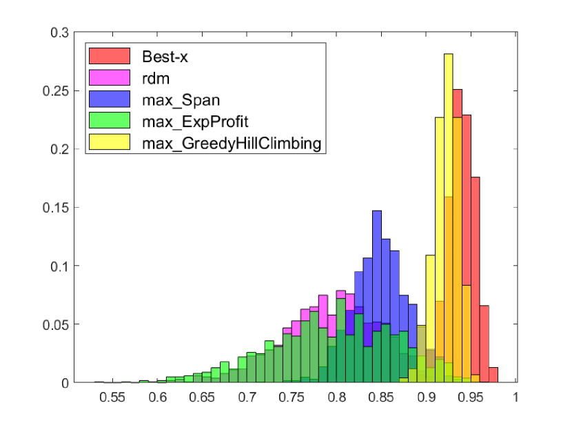
(a) $G^{(1)}=(1,0.95,0.9,\cdots,0.1,0.05)$

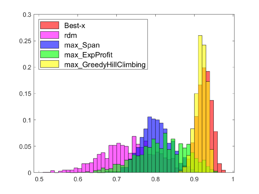
(b) $G^{(2)}=(1,0.9,0.9^{2},\cdots,0.9^{19})$

Figure 2: The histogram of 1000 instances for the performance of Best-x and other benchmarks relative to the clairvoyant upper bound under $G^{(1)}$ and $G^{(2)}$.

6.2 RankUCB

Next, we investigate the performance of Algorithm 5 RankUCB. In this experiment, we adopt a similar setting to that in Section 6.1. In particular, we consider 1000 products and $M=20$. We implement the RankUCB for 10 independent simulations, each with 10000 customers arriving sequentially. For each customer, her attention span has a geometric distribution $G^{(1)}$ from setting one in the last section, unknown to the firm. We conduct 10 simulation instances. At the beginning of each simulation instance, we randomly generate the prices of the products uniformly from $[0,10]$ and their features $s_{j}\sim\mathcal{N}(0.25,\mathbf{I}_{d_{p}\times d_{p}})\in\mathbb{R}^{d_{p}}$ with $d_{p}=10$. The product features are then normalized to $\|s_{j}\|_{2}=1$. In each round, we randomly generate the customer feature $y_{t}\sim\mathcal{N}(1,0.1\times\mathbf{I}_{d_{p}\times d_{p}})\in\mathbb{R}^{d_{c}}$ with $d_{c}=5$ and also normalize it to $\|y_{t}\|_{2}=1$. We generate $\theta^{*}\sim\mathcal{N}(0.25,\mathbb{I}_{50\times 50})$ and then normalized such that $\|\theta^{*}\|_{2}=0.906$. The same $\theta^{*}$ remains the same for the 10 independent simulations. In this setup, for any product $j$, it is guaranteed that the conditional purchase probability $|\lambda_{t,j}|\leq 0.906$.

Because of the dimension of the problem, the instances tend to have high variances due to the random draw of the feature vectors. To show the performance, we use a different measure than the regret. In particular, in each round we calculate the expected revenue of the ranking suggested by RankUCB conditional on the feature $x_{t,j}$ and thus the conditional purchase probabilities. Then we calculate the ratio over the conditionally expected revenue of the Best-x Algorithm (Algorithm 3) when all the information is known. The expected revenue instead of the realized revenue helps smooth the performance. Figure 3 illustrates the ratio over 10000 rounds as well as the standard error of 10 simulations. As we can observe, the expected reward of RankUCB increases to around 90% in 10000 rounds. This demonstrates its practical efficiency even under high dimensions $d=50$.

Figure 3: Performance ratio of RankUCB over 10000 rounds.

We also investigate the learning of the failure rate in the experiment. In particular, we show the point estimator $\hat{h}_{t,k}$ and the optimistic estimator $\hat{h}_{t,k}^{L}$ for the failure rate $h_{k}^{*}$ at $k\in\left\{1,3,5,10,15,19\right\}$. We plot the absolute errors relative to the actual value $h_{k}^{\ast}\equiv 0.05$. The results are illustrated in Figure 4.

Figure 4: Estimated failure rate in the learning process.

From Figure 4, we observe that the estimators for smaller $k$ converge faster, because there is less censoring for products ranked at the front. The optimistic estimators converge much slower than the point estimators, because of the slow decay of the confidence region. In particular, $\hat{h}_{t,1}^{L}$, $\hat{h}_{t,3}^{L}$ and $\hat{h}_{t,3}^{L}$ are very accurate over after 5000 rounds, while $\hat{h}_{t,10}^{L}$, $\hat{h}_{t,15}^{L}$ and $\hat{h}_{t,19}^{L}$ are still too optimistic after 10000 rounds. Nevertheless, as $T$ increases, the convergence of the estimates is reflected in the experiment.

7 Conclusion

In this paper, we study the revenue maximization problem of an online retailer, when customers browse the ranked products in order. The model extends the well-known cascade model in two directions: customers may have random attention spans, and the products have different prices. Based on the structure of the optimal ranking under fixed attention span, we develop an approximation algorithm with $1/e$-approximation ratio. When the conditional purchase probabilities of the products (which may be based on customer and product features) and the distribution of customers’ attention spans are unknown , we provide a learning algorithm that can effectively learn the parameters and achieve near-optimal $\tilde{\mathcal{O}}(\sqrt{T})$ regret. Our study addresses the two major challenges of the product ranking model when the firm is interested in revenue instead of click maximization.

Endnotes

1. 1 We use $|S|$ ($|\sigma|$) to represent the number of products in the assortment (ranking).
2. 2 We assume $\lambda_{j}\in(0,1]$ and $r_{j}>0$ for all $j$ because removing products with zero conditional purchase probability or zero price from the list does not affect the results.
3. 3 We have also tested two simple heuristics: max_Profit, displaying the 20 most profitable products (with the highest prices) and max_Choice, displaying the 20 products with the highest purchase probabilities. Both heuristics perform badly compared to others and we thus do not include them in the results.

Appendix

Appendix A Proofs in Section 4

Proof of Lemma 4.1: For the simplicity of notations, let us assume that $S=\left\{1,\dots,x\right\}$. Suppose in the ranking $\sigma$ there exists $i\in\left\{1,\dots,x-1\right\}$ such that $r_{\sigma(i)}<r_{\sigma(i+1)}$. We will argue that we can strictly improve the expected revenue by swapping the two products without changing the positions of other products. Consider the new ranking $\sigma^{\prime}$ with $\sigma^{\prime}(i)=\sigma(i+1)$, $\sigma^{\prime}(i+1)=\sigma(i)$, and $\sigma^{\prime}(k)=\sigma(k)$ for all other $k$. Let $\pi_{\sigma(i)}(\sigma)\triangleq\prod_{s=1}^{i-1}\big{(}1-\lambda_{\sigma(s)}\big{)}$ be the probability that the customer views product $\sigma(i)$. By definition, it is easy to see $\pi_{\sigma(k)}(\sigma)=\pi_{\sigma^{\prime}(k)}(\sigma^{\prime})$ for $k=1,\dots,i,i+2,\dots,x$. Therefore, the expected revenues generated from products in position $k$ are equal under $\sigma$ and $\sigma^{\prime}$ for $k=1,\dots,i-1,i+2,\dots,x$, recalling formula (2).

In order to show $R(\sigma^{\prime},x)>R(\sigma,x)$, it suffices to compare the revenues generated from the products in position $i$ and $i+1$ under the two rankings:

$$\pi_{\sigma(i)}(\sigma)\lambda_{\sigma(i)}r_{\sigma(i)}+\pi_{\sigma(i+1)}(\sigma)\lambda_{\sigma(i+1)}r_{\sigma(i+1)}<\pi_{\sigma^{\prime}(i)}(\sigma^{\prime})\lambda_{\sigma^{\prime}(i)}r_{\sigma^{\prime}(i)}+\pi_{\sigma^{\prime}(i+1)}(\sigma^{\prime})\lambda_{\sigma^{\prime}(i+1)}r_{\sigma^{\prime}(i+1)}.$$

This is indeed the case because

$$\pi_{\sigma(i)}(\sigma)\cdot r_{\sigma(i)}\lambda_{\sigma(i)}+\pi_{\sigma(i+1)}(\sigma)\cdot r_{\sigma(i+1)}\lambda_{\sigma(i+1)}$$

$$= \pi_{\sigma(i)}(\sigma)\Big{(}r_{\sigma(i)}\cdot\lambda_{\sigma(i)}+(1-\lambda_{\sigma(i)}\big{)}\cdot r_{\sigma(i+1)}\cdot\lambda_{\sigma(i+1)}\Big{)}$$

$$= \pi_{\sigma(i)}(\sigma)\Big{(}r_{\sigma(i+1)}\cdot\lambda_{\sigma(i+1)}+r_{\sigma(i)}(1-\lambda_{\sigma(i+1)})\cdot\lambda_{\sigma(i)}+(r_{\sigma(i)}-r_{\sigma(i+1)})\lambda_{\sigma(i)}\lambda_{\sigma(i+1)}\Big{)}$$

$$< \pi_{\sigma(i)}(\sigma)\Big{(}r_{\sigma(i+1)}\cdot\lambda_{\sigma(i+1)}+r_{\sigma(i)}(1-\lambda_{\sigma(i+1)}\big{)}\cdot\lambda_{\sigma(i)}\Big{)}$$

$$= \pi_{\sigma^{\prime}(i)}(\sigma^{\prime})\cdot r_{\sigma^{\prime}(i)}\lambda_{\sigma^{\prime}(i)}+\pi_{\sigma^{\prime}(i+1)}(\sigma^{\prime})\cdot r_{\sigma^{\prime}(i+1)}\lambda_{\sigma^{\prime}(i+1)}.$$

The inequality is because $r_{\sigma(i)}-r_{\sigma(i+1)}<0$ and $1>\lambda>0$. Therefore, $\sigma$ cannot be optimal and we have completed the proof.

 

Proof of Proposition 4.2: First of all, we show $\sigma_{j}^{k}$ is the optimal display of selecting $k$ products from $\{j,j+1,\cdots,n\}$ based on the recursive relationship in dynamical programming, with corresponding revenue $H_{j}^{k}$.

For $x=1$, we can see $H_{j}=\max_{s\geq j}r_{s}\lambda_{s}$, which exactly represents the maximum reward obtained by displaying one product from $\{j,j+1,\cdots,n\}$. Meanwhile, for any arbitrary $x\leq n$, we can see $\sigma_{n-x+1}^{x}=\{n-x+1,n-x+2,\cdots,n\}$, which displays $x$ products the last $x$ ones. Thus, $H_{n-x+1}^{x}$ is also optimal for $x\leq n$. We use these two scenarios as the base case, and prove the claim by induction. In particular, we show that if both $\sigma_{j+1}^{x}$ and $\sigma_{j}^{x-1}$ are optimal displays, then $\sigma_{j}^{x}$ is also optimal.

Recall the recursive relationship (6) that

$$H_{j}^{x}=\max\Big{(}r_{j}\lambda_{j}+(1-\lambda_{j})H_{j+1}^{x-1},H_{j+1}^{x}\Big{)}.$$

Suppose $\sigma_{j}^{x}$ is not optimal, then there must exist another display $\tilde{\sigma}_{j}^{x}$ with corresponding expected reward $\tilde{H}_{j}^{x}>H_{j}^{x}$. We consider two scenarios: (i) Suppose $j\in\tilde{\sigma}_{j}^{x}$, let $\tilde{\sigma}_{j}^{x}[2,x]$ be the display from the second product of $\sigma_{j}^{x}$ containing $(x-1)$ products with reward $R(\tilde{\sigma}_{j}^{x}[2,x],x-1)$, then we have

$$\tilde{H}_{j}^{x}=r_{j}\lambda_{j}+(1-\lambda_{j})R(\tilde{\sigma}_{j}^{x}[2,x],x-1)>H_{j}^{x}\geq r_{j}\lambda_{j}+(1-\lambda_{j})H_{j+1}^{x-1},$$

which implies $R(\tilde{\sigma}_{j}^{x}[2,x],x-1)>H_{j+1}^{x-1}$ and $\sigma_{j}^{x}[2,x]$ yields higher reward than $\sigma_{j+1}^{x-1}$. This contradicts the optimality of $\sigma_{j+1}^{x-1}$. (ii) Suppose $j\notin\tilde{\sigma}_{j}^{x}$, we have $\tilde{\sigma}_{j}^{x}=\sigma_{j+1}^{x}$, which also contradicts the assumption that $\tilde{H}_{j}^{x}>H_{j}^{x}\geq H_{j+1}^{x}$. Combining both cases, we conclude that $\sigma_{j}^{x}$ is also optimal and completes the induction proof.

Next, it suffices to show that $\sigma_{j}^{k}$ preserves the least lexicographic value to ensure $\sigma_{j}^{k}$ is $\mathcal{L}$-optimal. We use induction to prove that for any $1\leq k\leq n$, $\sigma_{j}^{k}$ is the $\mathcal{L}$-optimal display of selecting $k$ products from $\{j,j+1,\cdots,n\}$.

For $k=1$, let $\sigma_{j}^{1}=\{s\}$ be the solution returned by Algorithm 1 for $1\leq j\leq s\leq n$, based on the recursive relationship (6), we can see $\lambda_{u}r_{u}<\lambda_{s}r_{s}$ for all $j\leq u\leq s-1$, and $\lambda_{v}r_{v}\leq\lambda_{s}r_{s}$ for all $s+1\leq v\leq n$. Hence, $\sigma_{j}^{1}$ is $\mathcal{L}$-optimal for any $1\leq j\leq n$.

Next, suppose that argument is true for $k$. That is, $\sigma_{j}^{k}$ is $\mathcal{L}$-optimal for all $1\leq j\leq n-k+1$, we show that $\sigma_{j}^{k+1}$ is also $\mathcal{L}$-optimal for $1\leq j\leq n-k$.

Suppose $\sigma_{j}^{k+1}$ is not $\mathcal{L}$-optimal, then there exists a size-$(k+1)$ display $\tilde{\sigma}_{j}^{k+1}$ among products $\{j,j+1,\cdots,n\}$ that preserves same expected revenue $\tilde{H}_{j}^{k+1}=H_{j}^{k+1}$ (as $\sigma_{j}^{k+1}$ is optimal) but smaller lexicographic value than $\sigma_{j}^{k+1}$. Let $s_{1}=\min\{s,s\in\sigma_{j}^{k+1}\}$ and $\tilde{s}_{1}=\min\{\tilde{s},\tilde{s}\in\tilde{\sigma}_{j}^{k+1}\}$ be the item placed on the first position of $\sigma_{j}^{k+1}$ and $\tilde{\sigma}_{j}^{k+1}$ respectively. There are three scenarios to consider: (i) Suppose $\tilde{s}_{1}<s_{1}$, based on the dynamic programming relationship (6), we can see

$$\tilde{H}_{j}^{k+1}=\lambda_{\tilde{s}_{1}}r_{\tilde{s}_{1}}+(1-\lambda_{\tilde{s}_{1}})H_{{\tilde{s}_{1}}+1}^{k}<\lambda_{s_{1}}r_{s_{1}}+(1-\lambda_{s_{1}})H_{s_{1}+1}^{k}=H_{j}^{k+1},$$

which contradicts the $\mathcal{L}$-optimality of $\tilde{\sigma}_{j}^{k+1}$. (ii) Suppose $\tilde{s}_{1}>s_{1}$, the lexicographic value of $\tilde{\sigma}_{j}^{k+1}$ is indeed strictly higher than $\sigma_{j}^{k+1}$, which also contradicts the $\mathcal{L}$-optimality of $\tilde{\sigma}_{j}^{k+1}$. (iii) Suppose $\tilde{s}_{1}=s_{1}$ that the lexicographic value of the items placed on the first position of $\sigma_{j}^{k+1}$ and $\tilde{\sigma}_{j}^{k+1}$ are the same. Let $\tilde{\sigma}_{s_{1}+1}^{k}$ be the display from 2nd to the last position of $\tilde{\sigma}_{j}^{k+1}$, we can see that $\tilde{\sigma}_{s_{1}+1}^{k}\neq\sigma_{s_{1}+1}^{k}$, otherwise we have $\tilde{\sigma}_{j}^{k+1}\mathrel{\mathop{\ordinarycolon}}=\{s_{1}\}\cup\tilde{\sigma}_{s_{1}+1}^{k}=\{s_{1}\}\cup\sigma_{s_{1}+1}^{k}=\mathrel{\mathop{\ordinarycolon}}\sigma_{j}^{k+1}$. As $\sigma_{s_{1}+1}^{k}$ is $\mathcal{L}$-optimal from the induction argument, the lexicographic value of $\sigma_{s_{1}+1}^{k}$ is strictly less than that of $\tilde{\sigma}_{s_{1}+1}^{k}$, which also contradicts the assumption that $\tilde{\sigma}_{j}^{k+1}$ is $\mathcal{L}$-optimal. Combing all three scenarios above, we conclude that $\sigma_{j}^{k+1}$ is also $\mathcal{L}$-optimal, which completes the induction proof.    

Proof of Proposition 4.3:

In order to lay out the main idea of the proof, we first introduce some notations. Recall $H_{j}^{x}$ is the optimal revenue for customers with attention span $x$, when the products are chosen from $\{j,j+1,\dots,n\}$. Note that $j$ and $x$ satisfy $j+x\leq n+1$ for the problem to be non-trivial. Otherwise, we just display all products. Similarly, let $\sigma_{j}^{x}$ denote the corresponding $\mathcal{L}$-optimal ranking. By Lemma 4.1, the products in $\sigma_{j}^{x}$ are ordered by decreasing prices. We first prove the base case for the induction:

Claim: $\sigma_{n-2}^{1}\subset\sigma_{n-2}^{2}\subset\sigma_{n-2}^{3}$.

We state the proof for the claim below. Since the products are chosen from $\{n-2,n-1,n\}$, the ranking $\sigma_{n-2}^{3}$ includes all products and thus $\sigma_{n-2}^{2}\subset\sigma_{n-2}^{3}$. To show $\sigma_{n-2}^{1}\subset\sigma_{n-2}^{2}$, first consider the case $\sigma_{n-2}^{1}=\{n-2\}$. It implies that $r_{n-2}\lambda_{n-2}\geq\max\{r_{n-1}\lambda_{n-1},r_{n}\lambda_{n}\}$ because it is optimal to display product $n-2$ when customers have attention span fixed at one. If $n-2\notin\sigma_{n-2}^{2}$, then we have $\sigma_{n-2}^{2}=\{n-1,n\}$. By Lemma 4.1 and (1), the optimal ranking has the same order as the indices of the products in it. Therefore, with a slight abuse of notation, we simply use a set to denote the ranking, which is non-ambiguous. If we replace product $n$ in the second position of $\sigma_{n-2}^{2}$ by product $n-2$, the expected revenue conditional on the event that the customer doesn’t choose product $n-1$ in the first position is $r_{n-2}\lambda_{n-2}$, no less than $r_{n}\lambda_{n}$ which is the conditional expected revenue of product $n$. Therefore, $\sigma_{n-2}^{2}=\{n-1,n\}$ cannot be $\mathcal{L}$-optimal and we conclude that $n-2\in\sigma_{n-2}^{2}$. This implies $\sigma_{n-2}^{1}\subset\sigma_{n-2}^{2}$. Similar argument can be applied to the cases $\sigma_{n-2}^{1}=\{n-1\}$ or $\{n\}$. Therefore, we have completed the proof for the claim.

Now that we have proved the base case, the next lemma serves as the induction step.

Consider the $\mathcal{L}$-optimal assortment $\sigma_{j}^{x}$ of choosing $x$ products from $\{j,j+1,\cdots,n\}$, as there are $n-j+1$ products available among $\{j,j+1,\cdots,n\}$, we can see $1\leq x\leq n-j+1$. The following lemma states that if the $\mathcal{L}$-optimal displays among $\{j,j+1,\cdots,n\}$ preserve a nested structure, then the $\mathcal{L}$-optimal displays among $\{j-1,j,j+1,\cdots,n\}$ must follow such a nested structure as well.

Lemma A.1

Given $j\in\{2,3,\cdots,n-2\}$, for any $\mathcal{L}$-optimal assortment $\sigma_{j}^{x}$ of choosing $x$ products from $\{j,j+1,\cdots,n\}$ with $1\leq x\leq n-j+1$, if they are nested such that $\sigma_{j}^{1}\subset\sigma_{j}^{2}\subset\cdots\sigma_{j}^{n-j+1}$ , then the $\mathcal{L}$-optimal displays among products $\{j-1,j,\cdots,n\}$ are also nested, i.e., $\sigma_{j-1}^{1}\subset\sigma_{j-1}^{2}\subset\cdots\subset\sigma_{j-1}^{n-j+2}$.

With Lemma A.1, we are able to show Proposition 4.3 recursively.

Before proving Lemma A.3 and Lemma A.1, we first provide a lemma characterizing the relationship between $H_{j}^{m}$ and $H_{j}^{m+1}$, which is frequently applied throughout our analysis.

Lemma A.2

For any $j=1,2,\cdots,n-1$ and $x=1,2,\cdots,n-j$, we have $H_{j}^{x}\leq H_{j}^{x+1}$.

Proof of Lemma A.2: Recall that $\sigma_{j}^{x}$ and $\sigma_{j}^{x+1}$ are the optimal $\mathcal{L}$-optimal ranking for $x$ and $x+1$ products respectively. Let $P_{0}=\prod_{s=1}^{x}(1-\lambda_{\sigma_{j}^{x}(s)})$ be the probability that no products are purchased within $\sigma_{j}^{x}$. Without loss of generality, for any product $k\geq j,k\notin\sigma_{j}^{x}$, by adding this product at the last position of $\sigma_{j}^{x}$, we can construct a ranking $\tilde{\sigma}_{j}^{x+1}$ such that $\tilde{\sigma}_{j}^{x+1}(s)=\sigma_{j}^{x}(s)$ for $s=1,2,\cdots,m$ and $\tilde{\sigma}_{j}^{x+1}(x+1)=k$. It is easy to see that

$$R(\tilde{\sigma}_{j}^{x+1},x+1)=R(\sigma_{j}^{x},x)+P_{0}\cdot\lambda_{k}r_{k}\geq R(\sigma_{j}^{x},x).$$

Due to the fact $|\tilde{\sigma}_{j}^{x+1}|=x+1$ and the optimality of $\sigma_{j}^{x+1}$, we also have $H_{j}^{x+1}=R(\sigma_{j}^{x+1},x+1)\geq R(\tilde{\sigma}_{j}^{x+1},x+1)$. Combining them together, we conclude that

$$H_{j}^{x+1}\geq R(\tilde{\sigma}_{j}^{x+1},x+1)\geq R(\sigma_{j}^{x},m)=H_{j}^{x},$$

which completes the proof.    

Lemma A.3

Given $j\in\{1,\dots,n-2\}$, if $\sigma_{j}^{1}\subset\sigma_{j}^{2}\subset\dots\subset\sigma_{j}^{n-j+1}$, then we have

$$H_{j}^{x+2}-H_{j}^{x+1}\leq H_{j}^{x+1}-H_{j}^{x},$$

for all $x=1,2,\ldots,n-j-1$.

Proof of Lemma A.3: Due to the condition of the lemma, we have $\sigma_{j}^{x}\subset\sigma_{j}^{x+1}\subset\sigma_{j}^{x+2}$. Let $u$ and $v$ be the two items added to the optimal ranking for attention span $x+1$ and $x+2$ involving products $\{j,j+1,\ldots,n\}$. That is,

$$\sigma_{j}^{x+1}=\sigma_{j}^{x}\cup\{u\}\text{ and }\sigma_{j}^{x+2}=\sigma_{j}^{x+1}\cup\{v\}.$$

Again, we treat a ranking as a set without ambiguity because of Lemma 4.1. Suppose on the contrary the result does not hold, that is,

$$H_{j}^{x+2}-H_{j}^{x+1}>H_{j}^{x+1}-H_{j}^{x}.$$ (17)

We consider the two scenarios $u<v$ and $u>v$ separately. Also recall that $H_{j}^{k}=R(\sigma_{j}^{k},k)$ for $k=x,x+1,x+2$.

• Suppose $u<v$ and let $x_{v}$ be the number of items displayed in $\sigma_{j}^{x+2}$ after item $v$. By Lemma 4.1, the products displayed after item $v$ are chosen from $\{v+1,v+2,\ldots,n\}$. Moreover, they must generate the optimal revenue conditional on the event that the customer does not purchase any product after viewing product $v$. Therefore, the sub-ranking after $v$ is $\sigma_{v+1}^{x_{v}}$ and the conditional expected revenue is $H_{v+1}^{x_{v}}$.

  Let $P_{1}$ be the probability that a customer views product $v$ in the ranking $\sigma_{j}^{x+2}$. Suppose product $v$ is inserted in the $i_{v}$-th position of $\sigma_{j}^{x+2}$, i.e., $\sigma_{j}^{x+2}(i_{v})=v$. Due to the fact that $\sigma_{j}^{x+2}=\sigma_{j}^{x+1}\cup\{v\}$ and $v$ is inserted after $u$ (because $u<v$ and Lemma 4.1), the probability of viewing the $i_{v}$-th item in $\sigma_{j}^{x+1}$ is also $P_{1}$. The expected revenues generated before the $i_{v}$-th product are identical in $\sigma_{j}^{x+1}$ and $\sigma_{j}^{x+2}$. Thus, we have

  $$H_{j}^{x+2}-H_{j}^{x+1}=P_{1}\cdot\Big{(}\lambda_{v}r_{v}+(1-\lambda_{v})H_{v+1}^{x_{v}}-H_{v+1}^{x_{v}}\Big{)}=P_{1}\cdot\Big{(}\lambda_{v}r_{v}-\lambda_{v}H_{v+1}^{x_{v}}\Big{)}.$$ (18)

  Moreover, combining (18) with Lemma A.2, we can see that $r_{v}\geq H_{v+1}^{x_{v}}$ because $P_{1}>0$ and $\lambda_{v}>0$.

  Let $\tilde{\sigma}_{j}^{x+1}=\sigma_{j}^{x}\cup\{v\}$. Note that $\tilde{\sigma}_{j}^{x+1}$ includes $x+1$ products and it is not the optimal ranking. But we arrange the product in the ascending order of their indices as Lemma 4.1. Let $\tilde{P}_{1}$ be the probability of viewing product $v$ in the ranking $\tilde{\sigma}_{j}^{x+1}$ for a customer of attention span $x+1$. Comparing $\tilde{\sigma}_{j}^{x+1}$ and $\sigma_{j}^{x+2}$, the product $u$ is inserted to $\tilde{\sigma}_{j}^{x+1}$ to turn it into $\sigma_{i}^{x+2}$. Because $u<v$, we have $P_{1}=(1-\lambda_{u})\tilde{P}_{1}\leq\tilde{P}_{1}$. Note that the expected revenue conditional on the event that a customer doesn’t purchase after viewing product $v$ in $\tilde{\sigma}_{j}^{x+1}$ is still $H_{v+1}^{x_{v}}$ as the sub-ranking after $v$ remains the same as $\sigma_{j}^{x+2}$.

  Now consider the expected revenue of $\tilde{\sigma}_{j}^{x+1}$ and $\sigma_{j}^{x}$, which removes product $v$ in the former ranking. We have

  $$R(\sigma_{i}^{x}\cup\{v\},x+1)-H_{i}^{x}=\tilde{P}_{1}\Big{(}\lambda_{v}r_{v}+(1-\lambda_{v})H_{v+1}^{x_{v}}-H_{v+1}^{x_{v}}\Big{)}=\tilde{P}_{1}\Big{(}\lambda_{v}r_{v}-\lambda_{v}H_{v+1}^{x_{v}}\Big{)}$$

  $$\geq P_{1}\Big{(}\lambda_{v}r_{v}-\lambda_{v}H_{v+1}^{x_{v}}\Big{)}=H_{j}^{x+2}-H_{j}^{x+1}>H_{j}^{x+1}-H_{j}^{x},$$

  where the first inequality follows from $P_{1}\leq\tilde{P}_{1}$ and $r_{v}-H_{v+1}^{x_{v}}\geq 0$, the last equality follows from (18), and the last inequality follows from (17). Therefore, we have $R(\sigma_{j}^{x}\cup\{v\},x+1)>H_{j}^{x+1})$, which contracts the $\mathcal{L}$-optimality of $\sigma_{j}^{x+1}$.

• Next consider the case $v<u$. Suppose there are $x_{v}$ items placed after $v$ in $\sigma_{j}^{x+2}$. Similarly, denote the sub-ranking as $\sigma_{v+1}^{x_{v}}$ and the expected reward as $H_{v+1}^{x_{v}}$. Define $P_{0}$ as the probability of viewing item $v$ under $\sigma_{j}^{x+2}$. Similar to (18), we have

  $$H_{j}^{x+2}-H_{j}^{x+1}=P_{0}(\lambda_{v}r_{v}-\lambda_{v}H_{v+1}^{x_{v}}).$$

  Consider the ranking $\tilde{\sigma}_{j}^{x+1}=\sigma_{j}^{x}\cup\{v\}$. The sub-ranking after $v$ in $\tilde{\sigma}_{j}^{x+1}$ is $\sigma_{v+1}^{x_{v}}\setminus\{u\}$, or equivalently $\sigma_{v+1}^{x_{v}-1}$. By Lemma A.2, we have $H_{v+1}^{x_{v}-1}\leq H_{v+1}^{x_{v}}$. Therefore, similar to (18), we have

  $$\begin{split}&R(\sigma_{j}^{x}\cup\{v\},x+1)-H_{j}^{x}\\ =&P_{0}(\lambda_{v}r_{v}-\lambda_{v}H_{v+1}^{x_{v}-1})\geq P_{0}(\lambda_{v}r_{v}-\lambda_{v}H_{v+1}^{x_{v}})=H_{j}^{x+2}-H_{j}^{x+1}>H_{j}^{x+1}-H_{j}^{x},\end{split}$$

  which implies that $R(\sigma_{j}^{x}\cup\{v\},x+1)>H_{j}^{x+1}$ and contradicts the $\mathcal{L}$-optimality of $\sigma_{j}^{x+1}$.

Combining both cases, we conclude $H_{j}^{x+2}-H_{j}^{x+1}\leq H_{j}^{x+1}-H_{j}^{x}$, which completes the proof.    

Proof of Lemma A.1: First, consider $\sigma_{j-1}^{1}$ which has a single product. Suppose $\sigma_{j-1}^{1}=\{u\}$ where $u\geq j-1$. We have $r_{u}\lambda_{u}\geq\max_{k\geq j-1}\{r_{k}\lambda_{k}\}$ and $r_{u}\lambda_{u}>\max_{k=j-1,\dots,u-1}\{r_{k}\lambda_{k}\}$ because of the $\mathcal{L}$-optimality of $\sigma_{j-1}^{1}$. Therefore, if $u\notin\sigma_{j-1}^{2}$, then we can replace the last product in $\sigma_{j-1}^{2}$ by $u$ to increase the expected revenue of $H_{j-1}^{2}$ or make it lexicographically less. As a result, we must have $u\in\sigma_{j-1}^{2}$ and $\sigma_{j-1}^{1}\subset\sigma_{j-1}^{2}$.

Next, we prove $\sigma_{j-1}^{x}\subset\sigma_{j-1}^{x+1}$ for $2\leq x\leq n-j$. We first consider the case $j-1\notin\sigma_{j-1}^{x}$. In this case, we have $\sigma_{j-1}^{x}=\sigma_{j}^{x}$ by their definitions. If $j-1\notin\sigma_{j-1}^{x+1}$, then we have $\sigma_{j-1}^{x+1}=\sigma_{j}^{x+1}$ and thus $\sigma_{j-1}^{x}\subset\sigma_{j-1}^{x+1}$ by the induction hypothesis. If $j-1\in\sigma_{j-1}^{x+1}$, then by the $\mathcal{L}$-optimality, we must have that product $j-1$ is displayed in the first position of $\sigma_{j-1}^{x+1}$. The sub-ranking from the second position onward in $\sigma_{j-1}^{x+1}$ must be equivalent to $\sigma_{j-1}^{x}$ to maximize the expected revenue. Therefore, we have $\sigma_{j-1}^{x}\subset\sigma_{j-1}^{x+1}$.

Now suppose $j-1\in\sigma_{j-1}^{x}$. Since $\sigma_{j-1}^{x}$ is $\mathcal{L}$-optimal, $j-1$ must be ranked the first and thus

$$H_{j}^{x}\leq H_{j-1}^{x}=\lambda_{j-1}r_{j-1}+(1-\lambda_{j-1})H_{j}^{x-1}.$$

If ${j-1}\in\sigma_{j-1}^{x+1}$, then $\sigma_{j-1}^{x}\subset\sigma_{j-1}^{x+1}$ can be proved by the induction hypothesis on the sub-rankings of $\sigma_{j-1}^{x}$ and $\sigma_{j-1}^{x+1}$ from the second position onward. Suppose $j-1\notin\sigma_{j-1}^{x+1}$. Based on the induction hypothesis that $\sigma_{j}^{x-1}\subset\sigma_{j}^{x}\subset\sigma_{j}^{x+1}$, there exist items $u,v\notin\sigma_{j}^{x-1}$ such that

$$\sigma_{j}^{x}=\sigma_{j}^{x-1}\cup\{u\},\,\,\,\sigma_{j}^{x+1}=\sigma_{j}^{x}\cup\{v\}.$$ (19)

Since we have assumed that $j-1\notin\sigma_{j-1}^{x+1}$, we must have $\sigma_{j-1}^{x+1}=\sigma_{j}^{x+1}$. Suppose that in $\sigma_{j-1}^{x+1}$ or $\sigma_{j}^{x+1}$ there are $x_{u}$ and $x_{v}$ items placed after items $u$ and $v$ respectively. Recall that $H_{u+1}^{x_{u}}$ and $H_{v+1}^{x_{v}}$ are the expected revenue obtained from items after $u$ and $v$. Since $\sigma_{j-1}^{x+1}$ is $\mathcal{L}$-optimal, the expected revenue strictly decreases if one replaces either $u$ or $v$ in $\sigma_{j-1}^{x+1}$ by item $j-1$. Conditional on the event that the customer views product $u$ (or $j-1$), we have

$$\begin{split}\lambda_{j-1}r_{j-1}+(1-\lambda_{j-1})H_{u+1}^{x_{u}}<&\lambda_{u}r_{u}+(1-\lambda_{u})H_{u+1}^{x_{u}},\\ \lambda_{j-1}r_{j-1}+(1-\lambda_{j-1})H_{v+1}^{x_{v}}<&\lambda_{v}r_{v}+(1-\lambda_{v})H_{v+1}^{x_{v}}.\end{split}$$

Note that $r_{j-1}\geq r_{u}\geq H_{u+1}^{x_{u}}$ (the first inequality is because of the indexing of the products; the second inequality is because all products in $\sigma_{u+1}^{x_{u}}$ have revenues lower than $r_{u}$) and $r_{j-1}\geq r_{v}\geq H_{v+1}^{x_{v}}$. Therefore, we have $\lambda_{j-1}<\lambda_{u}$ and $\lambda_{j-1}<\lambda_{v}$, which implies

$$1-\lambda_{j-1}>1-\lambda_{u},\text{ and }1-\lambda_{j-1}>1-\lambda_{v}.$$ (20)

Let $r^{*}\mathrel{\mathop{\ordinarycolon}}=r_{j-1}\lambda_{j-1}+(1-\lambda_{j-1})H_{j}^{x}$ be the expected revenue obtained by inserting item ${j-1}$ in the first position of ranking $\sigma_{j}^{x}$. Since $j-1\notin\sigma_{j-1}^{x+1}$, we have $r^{*}<H_{j}^{x+1}$. We will show that $r^{*}\geq H_{j}^{x+1}$ in the rest of analysis to yield a contradiction which proves that $j-1\in\sigma_{j-1}^{x+1}$.

Recall that $H_{j-1}^{x}=r_{j-1}\lambda_{j-1}+(1-\lambda_{j-1})H_{j}^{x-1}$. By definition, we have

$$r^{*}=r_{j-1}\lambda_{j-1}+(1-\lambda_{j-1})H_{j}^{x}=H_{j-1}^{x}+(1-\lambda_{j-1})(H_{j}^{x}-H_{j}^{x-1}).$$ (21)

As $\sigma_{j}^{x-1}\cup\{v\}$ is not $\mathcal{L}$-optimal for $\sigma_{j}^{x}$, we also have

$$R(\sigma_{j}^{x-1}\cup\{v\},x)\leq R(\sigma_{j}^{x},x)=H_{j}^{x}.$$

We consider two cases: $u<v$ and $u>v$.

1. Suppose $u<v$. Note that the difference $H_{j}^{x+1}-H_{j}^{x}$ is only caused by the products displayed after the inserted position of product $v$ (see (19)). Therefore, we have

   $$\begin{split}H_{j}^{x+1}-H_{j}^{x}=&\Pr(\text{viewing product }v\text{ in }\sigma_{j}^{x+1})\cdot(\lambda_{v}r_{v}+(1-\lambda_{v})H_{v+1}^{x_{v}}-H_{v+1}^{x_{v}})\\ =&\Pr(\text{viewing product }v\text{ in }\sigma_{i}^{x+1}\setminus\{u\})(1-\lambda_{u})\lambda_{v}(r_{v}-H_{{v}+1}^{x_{v}})\\ =&(1-\lambda_{u})\cdot\big{(}R(\sigma_{j}^{x-1}\cup\{v\},x)-H_{j}^{x-1}\big{)}\\ \leq&(1-\lambda_{u})(H_{j}^{x}-H_{j}^{x-1}),\end{split}$$ (22)

   In the first equality, we condition on the event that a customer views product $v$ in $\sigma_{j}^{x+1}$. In the second equality, because $u<v$, product $u$ is displayed before $v$ in $\sigma_{j}^{x+1}$ by Lemma 4.1. In the third equality, after excluding product $u$, we are comparing the revenues of $\sigma_{j}^{x-1}$ and $\sigma_{j}^{x-1}\cup\{v\}$. The inequality due to the suboptimality of $\sigma_{j}^{x-1}\cup\{j\}$ in (19). By (21), we have

   $$r^{*}= H_{j-1}^{x}+(1-\lambda_{j-1})(H_{j}^{x}-H_{j}^{x-1})>H_{j-1}^{x}+(1-\lambda_{u})(H_{j}^{x}-H_{j}^{x-1})$$

   $$\geq H_{j}^{x}+(H_{j}^{x+1}-H_{j}^{x})=H_{j}^{x+1},$$

   where the first inequality follows from (20), and the second inequality follows from (22) and $H_{j-1}^{x}\geq H_{j}^{x}$. Therefore, we have $r^{*}>H_{j}^{x+1}$ if $u<v$.

2. Suppose $v<u$. Similar to (22), we have

   $$\begin{split}&R(\sigma_{j}^{x-1}\cup\{v,u\},x+1)-R(\sigma_{j}^{x-1}\cup\{v\},x)=H_{j}^{x+1}-R(\sigma_{j}^{x-1}\cup\{v\},x)\\ =&\Pr(\text{viewing product }u\text{ in }\sigma_{j}^{x+1})\cdot\lambda_{u}(r_{u}-H_{u+1}^{x_{u}})\\ =&(1-\lambda_{v})\Pr(\text{viewing product }u\text{ in }\sigma_{j}^{x+1}\setminus\{v\})\cdot\lambda_{u}(r_{u}-H_{u+1}^{x_{u}})\\ =&(1-\lambda_{v})\cdot\Big{(}R(\sigma_{j}^{x-1}\cup\{u\},x)-H_{j}^{x-1}\Big{)}\\ =&(1-\lambda_{v})(H_{j}^{x}-H_{j}^{x-1}).\end{split}$$ (23)

   Again, by (21), we have

   $$r^{*}= H_{j-1}^{x}+(1-\lambda_{j-1})(H_{j}^{x}-H_{j}^{x-1})$$

   $$> H_{j-1}^{x}+(1-\lambda_{v})(H_{j}^{x}-H_{j}^{x-1})$$

   $$= H_{j-1}^{x}+H_{j}^{x+1}-R(\sigma_{j}^{x-1}\cup\{v\},x)\geq H_{j}^{x+1},$$

   where the first inequality follows from $1-\lambda_{j-1}>1-\lambda_{v}$ in (20), the second equality is by (23), and the third inequality follows from $R(\sigma_{j}^{x-1}\cup\{v\},x)\leq H_{j-1}^{x}$ (suboptimality of $\sigma_{j}^{x-1}\cup\{v\}$ for $\sigma_{j-1}^{x}$). We conclude that $r^{*}>H_{j}^{x+1}$ also holds if $v<u$.

Combining both cases, we have $r^{*}>H_{j}^{x+1}$, which yields a contradiction. Therefore, we conclude that $j-1\in\sigma_{j-1}^{x+1}$. By the previous analysis, it implies that $\sigma_{j-1}^{x}\subset\sigma_{j-1}^{x+1}$ and thus $\sigma_{j-1}^{1}\subset\sigma_{j-1}^{2}\subset\cdots\subset\sigma_{j-1}^{n-j+1}$. To see $\sigma_{j-1}^{n-j+1}\subset\sigma_{j-1}^{n-j+2}$, note that $\sigma_{j-1}^{n-j+2}=\{j-1,j,\cdots,n\}$ is the full collection of products and the inclusion holds automatically. This completes the proof.    

Proof A.4

Proof of Proposition 4.5: The proof is given in the text before the proposition.    

Proof A.5

Proof of Theorem 4.6: Let $l=\min\{i\,\,|\,\,i=1,2,\cdots,M,i\geq\mathbb{E}(X)\}$ be the minimum index such that $l\geq\mathbb{E}[X]$, and the corresponding display $\sigma^{l}=\argmax_{\sigma}R(\sigma,l)$. Consider the reward $R(\sigma^{l},l)$. Clearly, there exists a piecewise linear continuous function $r\mathrel{\mathop{\ordinarycolon}}[1,M]\rightarrow R^{+}$ such that

• $r(i)=R(\sigma^{i},i)$ for all $i=1,2,\cdots,M,$

• $r$ is concave and increasing over $[1,M]$.

Then we have

$$R(\sigma^{l},l)=r(l)\geq r(\mathbb{E}[X])\geq\mathbb{E}[r(X)]=\mathbb{E}[R(\sigma^{X},X)],$$

where the first inequality is due to the fact that $l\geq\mathbb{E}[X]$, the second inequality comes from the concavity of $r(\cdot)$, and the first and last equalities are due to the fact that $R(\sigma^{i},i)=r(i)$ for $i=1,\cdots,M$.

Let $h(x)$ be the failure rate at $x$, by definition, we have $h(x)=(G_{x}-G_{x+1})/G_{x}=1-G_{x+1}/G_{x}$, which implies $G_{x+1}=\big{(}1-h(x)\big{)}G_{x}$. Recursively apply this relationship, we have

$$\Pr(X\geq\mathbb{E}[X])=\Pr(X\geq l)=G_{l}=\big{(}1-h(l-1)\big{)}G_{l-1}=\prod_{x=1}^{l-1}(1-h(x)).$$

Next, we prove that $\Pr(X\geq l)\geq 1/e$ for all $X$ following IFR. Due to the IFR property, we have $h(1)\leq h(2)\leq\cdots h(l-1)\leq h(l)\leq\cdots\leq h(M-1)$. Consider the function $h$ such that $\Pr(X\geq\mathbb{E}[X])$ is minimized. Suppose there exists $i\leq l-1$ and $j\geq l$ such that $h(i)<h(j)$. As $\mathbb{E}[X]=\sum_{x=1}^{M}\Pr(X\geq x)$, we can always decrease $h(j)$ and increase $h(i)$ such that $\mathbb{E}[X]$ remains unchanged. In this way, $\Pr(X\geq\mathbb{E}[X])$ strictly decreases, which contradicts the optimality of $h$. Therefore, we conclude that $h(i)=h(j)$ for every $i\leq l-1$ and $j\geq l$, which implies that $h(1)=h(2)=\cdots=h(M-1)$ and $X$ must follow geometry distribution.

Suppose $X\sim\text{Geometric}(p)$. As $\mathbb{E}[X]=1/p$, we have

$$\Pr(X\geq l)=\Pr(X\geq\mathbb{E}[X])=(1-p)^{\lceil 1/p\rceil-1}\geq(1-p)^{1/p}\geq 1/e.$$

To summarize, we have $\max_{k}R(\sigma^{k},k)\geq R(\sigma^{l})G_{l}\geq G_{l}\cdot\mathbb{E}[R(\sigma^{*},X)]\geq 1/e\cdot\mathbb{E}[R(\sigma^{*},X)]$, which completes the proof.

 

Proof A.6

Proof of Proposition 4.7: We consider a sufficiently large $M$. Moreover, assume consumer attention spans have geometric distribution with success probability equal to $1-\alpha$. That is, $\mathbb{P}(X\geq k)=\alpha^{k-1}$ for $1\leq k\leq M$. It is clear that $X$ satisfies Assumption 4.2. Product one has $r_{1}=1$ and $\lambda_{1}=1$; and for the rest of the products $r_{j}=r>1$, $\lambda_{j}=\lambda$, and $r_{j}\lambda_{j}=1-\alpha$ for all $j$. We also have $1=\lambda_{1}r_{1}=\frac{\lambda_{j}r_{j}}{1-\alpha}>\frac{\lambda_{j}r_{j}}{1-\alpha(1-\lambda_{j})}$ for $j\geq 2$.

Suppose the optimal ranking contains product one. By Proposition 4.11 presented in Section 4.3, product one must be placed on the first position. Because $\lambda_{1}=1$, any random customer would not continue to view products beyond that, so that the expected revenue for this ranking is 1. Suppose on the contrary that the optimal ranking does not contain product 1, because other products are identical, an optimal ranking is to place product $j$ on position $j-1$, which yields an expected revenue

$$\begin{split}&r_{2}\lambda_{2}+(1-\lambda_{2})\lambda_{3}r_{3}G_{2}+\cdots+\prod_{j=2}^{M}(1-\lambda_{j})\cdot\lambda_{M+1}r_{M+1}G_{M}\\ &=(1-\alpha)+(1-\lambda_{2})(1-\alpha)\alpha+\cdots+\prod_{j=2}^{M}(1-\lambda_{j})\cdot(1-\alpha)\alpha^{M-1}\\ &\leq(1-\alpha)+(1-\alpha)\alpha+\cdots+(1-\alpha)\alpha^{M-1}=(1-\alpha)\frac{1-\alpha^{M}}{1-\alpha}<1.\end{split}$$

Clearly, such ranking is not optimal and the optimal ranking must contain product 1. We conclude that the optimal expected revenue $\max_{\sigma}\mathbb{E}[R(\sigma,X)]=1$.

In terms of the clairvoyant upper bound, the clairvoyant retailer would set the following ranking for customers with attention span $x$: display product one in position $x$ and display other (identical) products in position one to $x-1$. In this case, the optimal revenue for customers with attention span $x=1$ is 1. Similarly, the optimal revenue for customers with attention span $x=2$ is $2-\alpha-\lambda$, by displaying product two in position one and product one in position two. Observe that the revenue is monotonically decreasing with respect to $\lambda$, the purchase probability of product two, so the revenue is maximized when $\lambda\rightarrow 0$. Then the expected revenue for customer with $x=2$ is arbitrarily close to $2-\alpha$. Using the same argument, we can argue that for customer with attention span $x$, the maximal expected revenue is $x-(x-1)\alpha$, which can be attained when $\lambda\rightarrow 0$. As a result, noting that the fraction of customers with attention span $x$ is $\alpha^{x-1}(1-\alpha)$, the clairvoyant upper bound is

$$\sum_{x=1}\big{(}x-(x-1)\alpha\big{)}\alpha^{x-1}(1-\alpha)=1+\alpha,$$

which is maximized when $\alpha\rightarrow 1$. Therefore, the clairvoyant upper bound can be arbitrarily close to 2. Since the optimal revenue for random attention spans is 1, no algorithm can achieve a performance ratio better than $1/2$ with respect to the clairvoyant upper bound.    

Proof A.7

Proof of Proposition 4.10: We first show the only if part. Suppose $\sigma^{M}$ is the optimal ranking under attention span $M$. Clearly $\sigma^{k}$ contains exactly the first $k$ items within $\sigma^{M}$. In particular, we have $\sigma^{1}=\sigma^{M}(1)$. In this case, to maximize the expected revenue of the single product, we must have $\sigma^{M}(1)=\max_{j}\lambda_{j}r_{j}$.

Then we consider $\sigma^{2}$, whose first item has been determined as $\sigma^{M}(1)$. Conditional on a customer with $x=2$ not buying the first item, clearly the second item $j$ should maximize the conditional expected revenue $\lambda_{j}r_{j}$ among the remaining products. Moreover, by Lemma 4.1, we must have $\sigma^{2}(2)=\max_{j>\sigma^{1}(1)}\lambda_{j}r_{j}$. That implies $i_{1}<i_{2}$. By iteratively applying this process, we conclude that we must have $i_{1}<i_{2}<\dots<i_{M}$.

Next we show the if part. We use mathematical induction in $M$ to show the claim that if $i_{1}<i_{2}<\dots<i_{M}$, then $\sigma^{k}$ is a prefix of $\sigma^{k+1}$ for $1\leq k\leq M-1$. For $M=1$, the claim is degenerate and always true. Suppose the claim holds for $M\leq n$. For $M=n+1$, by the inductive hypothesis, because $i_{1}<\dots<i_{n}$, we have $\sigma^{k}$ is a prefix of $\sigma^{k+1}$ for $k=1,\dots,n-1$ and $\sigma^{k}=\{i_{1},\dots,i_{k}\}$ for $k=1,\dots,n$. To show $\sigma^{n}$ is a prefix of $\sigma^{n+1}$, consider the first product in $\sigma^{n+1}$. If $\sigma^{n+1}(1)\coloneqq j<i_{1}$, then for the optimal ranking from position $2$ to $n+1$, we can consider a customer with attention span $n$. Since $i_{1}<\dots<i_{n}$, by the inductive hypothesis, this subranking is exactly $\sigma^{n}$. However, note that $\lambda_{j}r_{j}<\lambda_{i_{n+1}}r_{i_{n+1}}$ by the definition of $i_{n+1}$. Moreover, $\lambda_{j}<\lambda_{i_{n+1}}$ because $r_{j}>r_{i_{n+1}}$ since $j<i_{1}<i_{n+1}$ and by condition (1). It increases the revenue by replacing $j$ by $i_{n+1}$ due to the last but one equation of (5). This implies that $\sigma^{n+1}(1)\geq i_{1}$. By Proposition 4.3, $i_{1}\in\sigma^{n}\subset\sigma^{n+1}$. By Lemma 4.1 and the fact that $\sigma^{n+1}(1)\geq i_{1}$, we must have $\sigma^{n+1}(1)=i_{1}$. Now we consider the subranking from position 2 to $n+1$. Consider a customer with attention span $n$, because $i_{2}<\dots<i_{n+1}$, by the inductive hypothesis, we can infer that $\sigma^{n+1}(k)=i_{k}$ for $k=2,\dots,n+1$. This completes the inductive step and the claim.    

Proof A.8

Proof of Proposition 4.11: Let $G_{k}=\alpha^{k-1}$ for some $\alpha\in[0,1)$ and let $\sigma$ be the optimal ranking consisting of $M$ products. Assume there is a position $i<M$ such that $\frac{r_{\sigma(i)}\lambda_{\sigma(i)}}{1-\alpha(1-\lambda_{\sigma(i)})}<\frac{r_{\sigma(i+1)}\lambda_{\sigma(i+1)}}{1-\alpha(1-\lambda_{\sigma(i+1)})}$. Let $a=\sigma(i)$ and $a^{\prime}=\sigma(i+1)$ be two products in positions $i$ and $i+1$, respectively. We consider an alternative ranking that swaps $a$ and $a^{\prime}$ and leaves the positions of all other products unchanged. It is easy to see that the purchasing probabilities for all positions $j\notin\{i,i+1\}$ remain the same.

Let $C_{i}(\sigma)\triangleq\prod_{s=1}^{i-1}\big{(}1-\lambda_{\sigma(s)}\big{)}$. By swapping the positions of $a$ and $a^{\prime}$ and using the facts that $G_{i}=\alpha^{i-1}$ and $G_{i+1}=\alpha^{i}$, the total change in the expected reward is

$$C_{i}(\sigma)\Big{(}r_{a^{\prime}}\lambda_{a^{\prime}}G_{i}+r_{a}(1-\lambda_{a^{\prime}})\lambda_{a}G_{i+1}-r_{a}\lambda_{a}G_{i}-r_{a^{\prime}}(1-\lambda_{a})\lambda_{a^{\prime}}G_{i+1}\Big{)}$$

$$=C_{i}(\sigma)\Big{(}r_{a^{\prime}}\lambda_{a^{\prime}}(G_{i}-(1-\lambda_{a})G_{i+1})-r_{a}\lambda_{a}(G_{i}-(1-\lambda_{a^{\prime}})G_{i+1})\Big{)}$$

$$=\alpha^{i-1}C_{i}(\sigma)\Big{(}r_{a^{\prime}}\lambda_{a^{\prime}}(1-\alpha(1-\lambda_{a}))-r_{a}\lambda_{a}(1-\alpha(1-\lambda_{a^{\prime}}))\Big{)}\geq 0,$$

where the last inequality uses the assumption that $r_{a^{\prime}}\lambda_{a^{\prime}}(1-\alpha(1-\lambda_{a}))\geq r_{a}\lambda_{a}(1-\alpha(1-\lambda_{a^{\prime}}))$. Hence, swapping the position for $\sigma(i)$ and $\sigma(i+1)$ would increase the total revenue, which contradicts the optimality of this solution. This completes the proof.

 

Appendix B Proofs in Section 5

Proof of Lemma 5.3: This result follows standard techniques in linear cascade bandits, we present the details here for self-completeness. First of all, we consider the event $\{|x^{\top}(\theta^{*}-\hat{\theta}_{t})|\leq\rho_{t}\|x\|_{\mathbf{V}_{t}^{-1}},\,\,\forall\|x\|\leq 1\}$. Let $\mathcal{I}_{t}^{o}$ be the set of viewed products in round $t$. In particular, we have $\mathcal{I}_{t}^{o}=\{k|O_{t,k}^{Z}=1\}$. For any $t=1,2,\cdots$ and $k=1,2,\cdots,|\mathcal{I}_{t}^{o}|$, define

$$\eta_{t,k}=Z_{t,k}-x_{t,\sigma_{t}(k)}^{\prime}\theta^{*}.$$

As $\eta_{t,j}\in[-x_{t,\sigma_{t}(k)}^{\prime}\theta^{*},1-x_{t,\sigma_{t}(k)}^{\prime}\theta^{*}]$, we can see that $\eta_{t,j}$’s are bounded and $\frac{1}{2}$-subgaussian conditional on $\mathcal{F}_{t-1}$ and $y_{t}$ with $\mathbb{E}[\eta_{t,k}|\mathcal{F}_{t-1},y_{t}]=0$. Recall that $\mathbf{V}_{t}=\sum_{s=1}^{t}\sum_{k=1}^{|\mathcal{I}_{s}^{o}|}x_{s,\sigma_{t}(k)}x_{s,\sigma_{t}(k)}^{\top}+\gamma\mathbf{I}$ and $\|\theta^{*}\|_{2}\leq D$, by Theorem 2 in Abbasi-Yadkori et al. (2011), for any $\delta\in(0,1)$, we have

$$\|\hat{\theta}_{t}-\theta^{*}\|_{\mathbf{V}_{t}}\leq\sqrt{\frac{1}{2}\log\Big{(}\frac{\det(\mathbf{V}_{t})^{1/2}\det(\mathbf{V}_{0})^{-1/2})}{\delta}\Big{)}}+\gamma^{1/2}D,\,\,\,\forall t=0,1,\cdots$$

with probability at least $1-\delta$. Using trace-determinant inequality (Lemma 10 in Abbasi-Yadkori et al. (2011)) and the facts that $\|x_{s,\sigma_{s}(k)}\|^{2}\leq 1$ and $|\mathcal{I}_{t}^{o}|\leq M$, we have

$$\det(\mathbf{V}_{t})\leq\Big{(}\frac{\text{trace}(\mathbf{V}_{t})}{d}\Big{)}^{d}=\Big{(}\gamma+\frac{1}{d}\sum_{s=1}^{t}\sum_{k=1}^{|\mathcal{I}_{t}^{o}|}\|x_{s,\sigma_{s}(k)}\|^{2}\Big{)}^{d}\leq\Big{(}\gamma+tM/d\Big{)}^{d},$$

which further implies

$$\frac{\det(\mathbf{V}_{t})}{\det(\mathbf{V}_{0})}\leq\big{(}\frac{\gamma+tM/d}{\gamma}\big{)}^{d}=\big{(}1+\frac{tM}{\gamma d}\big{)}^{d}.$$

Finally, letting $\delta=1/t^{2}$, we obtain that with probability at least $1-1/t^{2}$,

$$\|\hat{\theta}_{t}-\theta^{*}\|_{\mathbf{V}_{t}}\leq\frac{1}{2}\sqrt{d\log\big{(}1+\frac{tM}{\gamma d}\big{)}+4\log(t)}+D\gamma^{1/2}=\rho_{t}.$$ (24)

Next, we consider the second part of the favorable event $\xi_{t}$. For any span $k$, as $Y_{t,k}$’s are a sequence of Bernoulli random variables with mean $h_{k}^{*}$, recall Hoeffding’s inequality, for any $\epsilon>0$, we have

$$\mathbb{P}(|\hat{h}_{t,k}-h_{k}^{*}|\leq\epsilon)\geq 1-\exp(-2\epsilon^{2}N_{t,k}).$$

Choosing $\epsilon=\sqrt{\ln(t)/N_{t,k}}$, we obtain

$$\mathbb{P}\Big{(}|\hat{h}_{t,k}-h_{k}^{*}|\leq\sqrt{\frac{\ln(t)}{N_{t,k}}}\Big{)}\geq 1-\exp(-2\ln(t))=1-1/t^{2}.$$

Applying the union bound for $k=1,2,\cdots,M-1$, together with (24), we have shown that $\mathbb{P}(\xi_{t})\geq 1-M/t^{2}$ and thus completes the proof.    

Next we outline the main idea behind the proof of Theorem 5.4. Recall the definition of the favorable event $\xi_{t}$ in Lemma 5.3. As a standard technique in UCB-type algorithms, we can decompose the regret in period $t$ by

$$\text{Reg}_{t}=\mathbb{E}[\text{Reg}_{t}\mathbb{I}_{\xi_{t-1}}]+\mathbb{E}[\text{Reg}_{t}\mathbb{I}_{\xi^{c}_{t-1}}]\leq\mathbb{E}[\text{Reg}_{t}\mathbb{I}_{\xi_{t-1}}]+\frac{r_{\max}M}{t^{2}}.$$

Here the regret from the unfavorable event $\xi_{t-1}^{c}$ can be bounded by the maximum revenue in a single period $r_{\max}$ and the probability $\mathbb{P}(\xi_{t-1}^{c})\leq M/t^{2}$ by Lemma 5.3.

To bound the regret from the favorable event, the standard approach is to show that when the parameters are optimistically estimated, the corresponding reward (revenue in our case) provides an upper bound for the actual reward as long as the true parameters fall into the confidence region. However, in our case, the optimistic estimators $G_{t,k}^{U}$ may not have IFR (see Assumption 4.2) anymore. It is not clear if the approximation algorithm in Step 7 of Algorithm 5 would still yield at least $1/e$ of the optimal revenue. Our next result addresses this concern.

Lemma B.1

We have

$$\mathbb{I}_{\xi_{t-1}}\mathbb{E}\left[\mathcal{R}(\sigma_{t};u_{t},G_{t}^{U})-\frac{1}{e}\mathcal{R}(\sigma^{*};\lambda_{t},G^{\ast})\bigg{|}\mathcal{F}_{t-1},y_{t}\right]\geq 0.$$

The term $\mathcal{R}(\sigma_{t};u_{t},G_{t}^{U})$ stands for the (conditionally) expected revenue according to the optimistic estimators and $\mathcal{R}(\sigma^{*};\lambda_{t},G^{\ast})$ is the optimal expected revenue for customer $t$. The latter is independent of $\mathcal{F}_{t-1}$ and depends on $y_{t}$ through $\lambda$.

Proof B.2

Proof of Lemma B.1: Suppose $u\geq\lambda$, we consider $G$ to be a decision variable and solve the optimal ranking $\tilde{\sigma}$ and $\tilde{G}$ that satisfies Assumption 4.2 and $\tilde{G}\leq G^{U}_{t}$ under choice probability $u$. That is,

$$\begin{split}(\tilde{\sigma},\tilde{G})=&\argmax_{\sigma,G}\sum_{k=1}^{M}\prod_{s=1}^{k-1}(1-u_{\sigma(s)})\cdot u_{\sigma(k)}r_{\sigma(k)}\cdot G_{k}\\ \mbox{s.t.}\,&G_{k}\leq G_{k}^{U}\,\,\text{ for }k=1,2,\cdots,M,\\ &G_{1},\cdots,G_{n}\text{ follow IFR}.\end{split}$$ (25)

Let $\{\sigma^{x}\}$’s be the solution return by AssortOpt with reward $r_{j}$’s and choice probability $u_{x}$’s, which is independent of span distribution. As $\tilde{G}$ follows IFR, we have

$$\max_{x}R(\sigma^{x},x;u)\tilde{G}_{x}\geq\frac{1}{e}\max_{\sigma}\sum_{x=1}^{M}\prod_{s=1}^{k-1}(1-u_{s})\cdot u_{x}\cdot r_{x}\cdot\tilde{G}_{x}=\frac{1}{e}\cdot\mathcal{R}(\tilde{\sigma};u,\tilde{G}).$$

On the other hand, the actual distribution $G$ and the corresponding optimal ranking $\sigma^{*}$ are also feasible for (25). As $u\geq\lambda$, it is thus easy to see that

$$\mathcal{R}(\sigma^{*};\lambda,G)\leq\mathcal{R}(\sigma^{*};u,G)\leq\mathcal{R}(\tilde{\sigma};u,\tilde{G}).$$

Combining them together, we have

$$\mathcal{R}(\sigma^{*};\lambda,G^{\ast})\leq\mathcal{R}(\tilde{\sigma};u,\tilde{G})\leq e\cdot\max_{x}R(\sigma^{x},x;u)\cdot\tilde{G}_{x}$$

$$\leq e\cdot\max_{x}R(\sigma^{x},x;u)\cdot G_{x}^{U}=e\cdot R(\sigma_{t},|\sigma_{t}|;u)G_{|\sigma_{t}|}^{U}\leq e\cdot\mathcal{R}(\sigma_{t};u,G^{U}),$$

where the third inequality is due to $\tilde{G}_{k}\leq G_{k}^{U}$ in (25) and the fourth inequality comes from the fact that $\sigma_{t}=\argmax_{\sigma^{x}\mathrel{\mathop{\ordinarycolon}}1\leq x\leq M}R(\sigma^{x},x;u)G_{x}^{U}$. This completes the proof.

Next, we introduce a lemma that will be used in the proof for Theorem 5.4.

Lemma B.3

Suppose $u\geq\lambda$ and $h^{L}\leq h^{*}$. Let $G_{k}^{U}=\prod_{i=1}^{k-1}(1-h_{i}^{L})$, we have

$$\begin{split}&\sum_{k=1}^{M}\Big{(}\prod_{i=1}^{k-1}(1-u_{i})\cdot u_{k}\cdot G_{k}^{U}-\prod_{i=1}^{k-1}(1-\lambda_{i})\cdot\lambda_{k}\cdot G_{k}^{*}\Big{)}r_{k}\\ \leq&\sum_{k=1}^{M}\mathbb{E}[O_{t,k}^{Y}]\cdot|h_{k}^{*}-h_{k}^{L}|\cdot r_{\max}+\sum_{k=1}^{M}\mathbb{E}[O_{t,k}^{Z}]\cdot|u_{k}-\lambda_{k}|\cdot r_{\max}.\end{split}$$

Proof of Lemma B.3: Given a ranking $\sigma_{t}$, conditional purchase probability $\lambda$, and failure rate $h$, for any $k\geq 1$, we have

$$\mathbb{P}(O_{t,k+1}^{Z}=1;\lambda,h)=(1-h_{k})\mathbb{P}[O_{t,k}^{Y}=1;\lambda,h]\text{ and }\mathbb{P}[O_{t,k}^{Y}=1;\lambda,h]=(1-\lambda_{k})\mathbb{P}[O_{t,k}^{Z}=1;\lambda,h].$$ (26)

We can see that

$$\begin{split}&\prod_{i=1}^{k-1}(1-u_{i})\cdot u_{k}\cdot G_{k}^{U}-\prod_{i=1}^{k-1}(1-\lambda_{i})\cdot\lambda_{k}\cdot G_{k}^{*}\\ =&\prod_{i=1}^{k-1}(1-u_{i})(1-h_{i}^{L})\cdot u_{k}-\prod_{i=1}^{k-1}(1-\lambda_{i})(1-h_{i}^{*})\cdot\lambda_{k}\\ =&\mathbb{P}[O_{t,k}^{Y}=1;u,h^{L}]\cdot u_{k}-\mathbb{P}[O_{t,k}^{Z}=1;\lambda,h^{*}]\cdot\lambda_{k}.\end{split}$$

To bound the right-hand side, by (26), we have

$$\begin{split}&\mathbb{P}[O_{t,k}^{Z}=1;u,h^{L}]\cdot u_{k}-\mathbb{P}[O_{t,k}^{Z}=1;\lambda,h^{*}]\cdot\lambda_{k}\\ =&\big{(}\mathbb{P}[O_{t,k}^{Z}=1;u,h^{L}]-\mathbb{P}[O_{t,k}^{Z}=1;\lambda,h^{*}]\big{)}\cdot u_{k}+\mathbb{P}[O_{t,k}^{Z}=1;\lambda,h^{*}]\cdot(u_{k}-\lambda_{k})\\ =&\big{(}\mathbb{P}[O_{t,k}^{Z}=1;u,h^{L}]-\mathbb{P}[O_{t,k}^{Z}=1;\lambda,h^{*}]\big{)}\cdot u_{k}+\mathbb{E}[O_{t,k}^{Z}]\cdot(u_{k}-\lambda_{k}).\end{split}$$ (27)

Then consider the term $\mathbb{P}[O_{t,k}^{Z}=1;u,h^{L}]-\mathbb{P}[O_{t,k}^{Z}=1;\lambda,h^{*}]$. we have

$$\begin{split}&\mathbb{P}[O_{t,k}^{Z}=1;u,h^{L}]-\mathbb{P}[O_{t,k}^{Z}=1;\lambda,h^{*}]\\ =&(1-h_{k-1}^{L})\cdot\mathbb{P}[O_{t,k-1}^{Y}=1;u,h^{L}]+(1-h_{k-1})\cdot\mathbb{P}[O_{t,k-1}^{Y}=1;\lambda,h^{*}]\\ =&(1-h_{k-1}^{L})\cdot\big{(}\mathbb{P}[O_{t,k-1}^{Y}=1;u,h^{L}]-\mathbb{P}[O_{t,k-1}^{Y}=1;\lambda,h^{*}]\big{)}+(h_{k-1}^{*}-h_{k-1}^{L})\cdot\mathbb{P}[O_{t,k-1}^{Y}=1;\lambda,h^{*}])\\ =&(1-h_{k-1}^{L})\cdot\big{(}\mathbb{P}[O_{t,k-1}^{Y}=1;u,h^{L}]-\mathbb{P}[O_{t,k-1}^{Y}=1;\lambda,h^{*}]\big{)}+\mathbb{E}[O_{t,k-1}^{Y}]\cdot(h_{k-1}^{*}-h_{k-1}^{L}).\end{split}$$ (28)

Furthermore, we have

$$\begin{split}&\mathbb{P}[O_{t,k-1}^{Y}=1;u,h^{L}]-\mathbb{P}[O_{t,k-1}^{Y}=1;\lambda,h^{*}]\\ =&(1-u_{k-1})\mathbb{P}[O_{t,k-1}^{Z}=1;u,h^{L}]-(1-\lambda_{k-1})\mathbb{P}[O_{t,k-1}^{Z}=1;\lambda,h^{*}]\\ =&(1-u_{k-1})\Big{(}\mathbb{P}[O_{t,k-1}^{Z}=1;u,h^{L}]-\mathbb{P}[O_{t,k-1}^{Z}=1;\lambda,h^{*}]\Big{)}+(\lambda_{k-1}-u_{k-1})\mathbb{P}[O_{t,k-1}^{Z}=1;\lambda,h^{*}]\\ \leq&(1-u_{k-1})\Big{(}\mathbb{P}[O_{t,k-1}^{Z}=1;u,h^{L}]-\mathbb{P}[O_{t,k-1}^{Z}=1;\lambda,h^{*}]\Big{)},\end{split}$$

where the last inequality comes from the fact that $\lambda\leq u$. Combining the preceding two inequalities together, we can see that

$$\begin{split}&\mathbb{P}[O_{t,k}^{Z}=1;u,h^{L}]-\mathbb{P}[O_{t,k}^{Z}=1;\lambda,h^{*}]\\ \leq&(1-h_{k-1}^{L})(1-u_{k-1})\Big{(}\mathbb{P}[O_{t,k-1}^{Z}=1;u,h^{L}]-\mathbb{P}[O_{t,k-1}^{Z}=1;\lambda,h^{*}]\Big{)}.\end{split}$$ (29)

Recursively applying this process, we obtain

$$\begin{split}\mathbb{P}[O_{t,k}^{Z}=1;u,h^{L}]-\mathbb{P}[O_{t,k}^{Z}=1;\lambda,h^{*}]\leq\mathbb{E}\Big{[}\sum_{j=1}^{k-1}O_{t,j}^{Y}\cdot|h_{j}^{*}-h_{j}^{L}|\cdot\big{(}\prod_{s=j+1}^{k-1}(1-u_{s})(1-h_{s}^{L})\big{)}\Big{]}.\end{split}$$ (30)

Plugging (30) into (27), we have

$$\begin{split}&\prod_{i=1}^{k-1}(1-u_{i})\cdot u_{k}\cdot G_{t,k}^{U}-\prod_{i=1}^{k-1}(1-\lambda_{j})\cdot\lambda_{k}\cdot G_{k}^{*}\\ \leq&\mathbb{E}\Big{[}\sum_{i=1}^{k-1}O_{t,i}^{Y}\cdot|h_{i}^{*}-h_{i}^{L}|\cdot\big{(}\prod_{s=i+1}^{k-1}(1-u_{s})(1-h_{s}^{L})\cdot u_{k}\big{)}+O_{t,k}^{Z}\cdot|u_{k}-\lambda_{k}|\Big{]}.\end{split}$$ (31)

Multiplying the corresponding profit $r_{k}$ and summing over $k=1,2,\cdots,M$, we can see that

$$\begin{split}&\sum_{k=1}^{M}\Big{(}\prod_{i=1}^{k-1}(1-u_{i})\cdot u_{k}\cdot G_{k}^{U}-\prod_{j=1}^{k-1}(1-\lambda_{i})\cdot\lambda_{k}\cdot G_{k}^{*}\Big{)}r_{k}\\ \leq&\sum_{k=1}^{M}\mathbb{E}\Big{[}\sum_{i=1}^{k-1}O_{t,i}^{Y}\cdot|h_{i}^{*}-h_{i}^{L}|\cdot\big{(}\prod_{s=i+1}^{k-1}(1-u_{s})(1-h_{s}^{L})\cdot u_{k}\big{)}+O_{t,k}^{Z}\cdot|u_{k}-\lambda_{k}|\Big{]}\cdot r_{k}\\ =&\sum_{k=1}^{M-1}\mathbb{E}[O_{t,k}^{Y}]\cdot|h_{k}^{*}-h_{k}^{L}|\cdot\underbrace{\Big{[}\sum_{i=k+1}^{M}\Big{(}\prod_{s=k+1}^{i-1}(1-u_{s})(1-h_{s}^{L})\cdot u_{i}\cdot r_{i}\Big{)}\Big{]}}_{Q_{k}}+\sum_{k=1}^{M}\mathbb{E}[O_{t,k}^{Z}]\cdot|u_{k}-\lambda_{k}|\cdot r_{k}.\end{split}$$

Also note that $O_{t,1}^{Y}=1$ always holds, which implies that the agent is always able to observe customer’s choice decision on the first item. Finally, consider the term $Q_{k}$, we can see

$$Q_{k}\triangleq\sum_{i=k+1}^{M}\Big{(}\prod_{s=k+1}^{i-1}(1-u_{s})(1-h_{s}^{L})\cdot u_{i}\cdot r_{i}\Big{)}=\mathbb{E}[\mathcal{R}(\sigma_{t};u,G^{U})|O_{k+1}^{Z}=1],$$

which is the conditional expected reward given that user views the $(k+1)$-th item under $u_{t},G^{u}$. Thus, a natural bound obtained for $Q_{k}$ is

$$Q_{k}\leq r_{\max}.$$

Plug this into the preceding relationship, we have

$$\begin{split}&\sum_{k=1}^{M}\Big{(}\prod_{i=1}^{k-1}(1-u_{i})\cdot u_{k}\cdot G_{k}^{U}-\prod_{i=1}^{k-1}(1-\lambda_{i})\cdot\lambda_{k}\cdot G_{k}^{*}\Big{)}r_{k}\\ \leq&\sum_{k=1}^{M-1}\mathbb{E}[O_{t,k}^{Y}]\cdot|h_{k}^{*}-h_{k}^{L}|\cdot r_{\max}+\sum_{k=1}^{M}\mathbb{E}[O_{t,k}^{Z}]\cdot|u_{k}-\lambda_{k}|\cdot r_{k},\end{split}$$

which completes the proof.    

Proof of Theorem 5.4: Let $\mathcal{F}_{t}$ be the $\sigma$-algebra of historical observations up to the end of round $t$, $y_{t}$ be the feature of user $t$, and $\sigma_{t}$ be the ranking displayed in round $t$. The favorable event is defined in Lemma 5.3

$$\xi_{t}=\Big{\{}\{\|\theta^{*}-\hat{\theta}_{t}\|_{\mathbf{V}_{t}}\leq\rho_{t}\}\cap\{h_{k}^{*}\geq\hat{h}_{t,k}-\sqrt{\ln(t)/N_{t,k}}\},\,\,\forall k=1,2,\cdots,M-1\Big{\}}.$$

By Lemma 5.3, we have $\mathbb{P}(\xi_{t})\geq 1-M/t^{2}$. Under $\xi_{t}$, we have $\lambda_{t,j}\leq u_{t,j}$ for each product $j$ and $h_{t,k}^{L}\leq h_{k}^{*}$ for all $k=1,2,\cdots,M$, which further implies $G_{t,k}^{U}\geq G_{k}^{*}$ for all $k=1,\cdots,M$.

Recall that $\text{Reg}_{t}$ is the scaled regret incurred in round $t$, as $\text{Reg}_{t}\leq r_{\max}$, given the customer feature $y_{t}$, we have

$$\begin{split}&\mathbb{E}[\text{Reg}_{t}|\mathcal{F}_{t-1},y_{t}]=\mathbb{E}[\mathcal{R}(\sigma^{*};\lambda_{t},G^{\ast})|y_{t}]-e\cdot\mathbb{E}[\mathcal{R}(\sigma_{t};\lambda_{t},G^{\ast})|\mathcal{F}_{t-1},y_{t}]\\ =&\mathbb{E}[\big{(}\mathcal{R}(\sigma^{*};\lambda_{t},G^{\ast})-e\cdot\mathbb{E}[\mathcal{R}(\sigma_{t};\lambda_{t},G^{\ast})\big{)}\cdot\mathbb{I}_{\xi_{t-1}}|\mathcal{F}_{t-1},y_{t}]+r_{\max}\cdot\mathbb{P}(\xi_{t-1}^{c})\\ \leq&\mathbb{E}[\big{(}\mathcal{R}(\sigma^{*};\lambda_{t},G^{\ast})-e\cdot\mathbb{E}[\mathcal{R}(\sigma_{t};\lambda_{t},G^{\ast})\big{)}\cdot\mathbb{I}_{\xi_{t-1}}|\mathcal{F}_{t-1},y_{t}]+\frac{Mr_{\max}}{t^{2}}\\ =&\mathbb{E}[\big{(}\mathcal{R}(\sigma^{*};\lambda_{t},G^{\ast})-e\cdot\mathcal{R}(\sigma_{t};u_{t},G_{t}^{U})\big{)}\cdot\mathbb{I}_{\xi_{t-1}}|\mathcal{F}_{t-1},y_{t}]+\frac{Mr_{\max}}{t^{2}}\\ &+\mathbb{E}[e\cdot\mathcal{R}(\sigma_{t};u_{t},G_{t}^{U})-e\cdot\mathbb{E}[\mathcal{R}(\sigma_{t};\lambda_{t},G^{\ast})\big{)}\cdot\mathbb{I}_{\xi_{t-1}}|\mathcal{F}_{t-1},y_{t}].\end{split}$$

Since $u_{t,j}\geq\lambda_{t,j}$ and $h_{t,k}^{L}\leq h_{k}^{*}$ under $\xi_{t-1}$, using Lemma B.1, we can see that

$$\mathbb{E}[e\cdot\mathcal{R}(\sigma_{t};u_{t},G_{t}^{U})\cdot\mathbb{I}_{\xi_{t-1}}|\mathcal{F}_{t-1},y_{t}]\geq \mathbb{E}[e\cdot\max_{x}R(\sigma_{t},x;u_{t},G_{t}^{U})\cdot\mathbb{I}_{\xi_{t-1}}|\mathcal{F}_{t-1},y_{t}]$$

$$\geq \mathbb{E}[\mathcal{R}(\sigma_{t};\lambda_{t},G^{*})\cdot\mathbb{I}_{\xi_{t-1}}|\mathcal{F}_{t-1},y_{t}],$$

so that the preceding inequality could be further expressed as

$$\mathbb{E}[\text{Reg}_{t}|\mathcal{F}_{t-1},y_{t}]\leq\mathbb{E}[e\cdot\mathcal{R}(\sigma_{t};u_{t},G_{t}^{U})-e\cdot\mathbb{E}[\mathcal{R}(\sigma_{t};\lambda_{t},G^{\ast})\big{)}\cdot\mathbb{I}_{\xi_{t-1}}|\mathcal{F}_{t-1},y_{t}]+\frac{Mr_{\max}}{t^{2}}.$$ (32)

Moreover, with the help of Lemma B.3, we have

$$\begin{split}&\mathbb{E}\Big{[}\big{(}\mathcal{R}(\sigma_{t};u_{t},G_{t}^{U})-\mathcal{R}(\sigma_{t};\lambda_{t},G^{\ast})\big{)}\cdot\mathbb{I}_{\xi_{t-1}}\Big{|}\mathcal{F}_{t-1},y_{t}\Big{]}\\ =&\sum_{x=1}^{M}\mathbb{E}\Big{[}\Big{(}\prod_{s=1}^{x-1}(1-u_{t,\sigma(s)})\cdot u_{t,\sigma_{t}(x)}G_{t,x}^{U}-\prod_{s=1}^{x-1}(1-\lambda_{t,\sigma_{t}(s)})\cdot\lambda_{t,\sigma_{t}(x)}\cdot G_{x}\Big{)}\cdot\mathbb{I}_{\xi_{t-1}}\Big{|}\mathcal{F}_{t-1},y_{t}\Big{]}\cdot r_{\sigma_{t}(x)}\\ \leq&r_{\max}\cdot\mathbb{E}\Big{[}\Big{(}\sum_{k=1}^{M}O_{t,k}^{Y}\cdot|h_{k}^{*}-h_{k}^{L}|+\sum_{k=1}^{M}O_{t,k}^{Z}\cdot|u_{k}-\lambda_{k}|\Big{)}\cdot\mathbb{I}_{\xi_{t-1}}\Big{|}\mathcal{F}_{t-1},y_{t}\Big{]}\\ \leq&2r_{\max}\cdot\mathbb{E}\Big{[}\Big{(}\underbrace{\sum_{k=1}^{M}O_{t,k}^{Y}\cdot\sqrt{\frac{\log(t-1)}{N_{t-1,k}}}}_{L_{t,1}}+\underbrace{\sum_{k=1}^{M}O_{t,k}^{Z}\cdot\rho_{t-1}\|x_{t,\sigma_{t}(k)}\|_{\mathbf{V}_{t-1}^{-1}}}_{L_{t,2}}\Big{)}\cdot\mathbb{I}_{\xi_{t-1}}\Big{|}\mathcal{F}_{t-1},y_{t}\Big{]},\end{split}$$

where the last inequality uses the fact that $|h_{k}^{*}-h_{t,k}^{L}|\leq 2|h_{k}^{*}-\hat{h}_{t,k}|\leq 2\sqrt{\frac{\ln(t-1)}{N_{t-1,k}}}$ and $|u_{t,\sigma_{t}(k)}-\lambda_{t,\sigma_{t}(k)}|\leq 2|x_{t,\sigma_{t}(k)}^{\top}(\theta^{*}-\hat{\theta}_{t-1})|\leq 2\rho_{t-1}\|x_{t,\sigma_{t}(k)}\|_{\mathbf{V}_{t-1}^{-1}}$ under the favorable event $\xi_{t-1}$. Let

$$L_{t,1}=\sum_{k=1}^{M}O_{t,k}^{Y}\cdot\sqrt{\frac{\ln(t-1)}{N_{t-1,k}}},\,\,L_{t,2}=\sum_{k=1}^{M}O_{t,k}^{Z}\cdot\rho_{t-1}\|x_{t,\sigma_{t}(k)}\|_{\mathbf{V}_{t-1}^{-1}}.$$

Plugging them into (32) and summing the scaled-regret over $t=1,2,\cdots,T$, we have

$$\begin{split}\sum_{t=1}^{T}\mathbb{E}[\text{Reg}_{t}]\leq&2e\cdot r_{\max}\mathbb{E}\Big{[}\sum_{t=1}^{T}(L_{t,1}+L_{t,2})\mathbb{I}_{\xi_{t-1}}\Big{]}+\sum_{t=1}^{T}\frac{2r_{\max}}{t^{2}}\\ \leq&2e\cdot r_{\max}\mathbb{E}\Big{[}\sum_{t=1}^{T}(L_{t,1}+L_{t,2})\mathbb{I}_{\xi_{t-1}}\Big{]}+\frac{M\pi^{2}r_{\max}}{6},\end{split}$$

where the last inequality uses the fact that $\sum_{t=1}^{\infty}1/t^{2}=\pi^{2}/6$. The rest of our analysis is to bound both $\sum_{t=1}^{T}\mathbb{E}[L_{t,1}\cdot\mathbb{I}_{\xi_{t-1}}]$ and $\sum_{t=1}^{T}\mathbb{E}[L_{t,2}\cdot\mathbb{I}_{\xi_{t-1}}]$. Firstly, consider $\sum_{t=1}^{T}\mathbb{E}[L_{t,1}\cdot\mathbb{I}_{\xi_{t-1}}]$, we have

$$\begin{split}\sum_{t=1}^{T}L_{t,1}=&\sum_{t=1}^{T}\sum_{k=1}^{M}O_{t,k}^{Y}\cdot\sqrt{\frac{\ln(t-1)}{N_{t-1,k}}}\\ \leq&\sum_{k=1}^{M}\int_{s=1}^{N_{t-1,k}+1}\sqrt{\frac{\ln T}{s}}ds\\ \leq&2M\sqrt{(N_{t-1,k}+1)\ln T}\leq 2M\sqrt{T\ln T}.\end{split}$$

Consequently, we have

$$\sum_{t=1}^{T}\mathbb{E}[L_{t,1}\cdot\mathbb{I}_{\xi_{t-1}}]\leq\mathbb{E}[\sum_{t=1}^{T}L_{t,1}]\leq 2M\sqrt{(N_{t-1,k}+1)\ln T}\leq 2M\sqrt{T\ln T},$$ (33)

where the first inequality is due to the fact that $L_{t,1}\geq 0$. Next consider $\sum_{t=1}^{T}\mathbb{E}[L_{t,2}\mathbb{I}_{\xi_{t-1}}]$, using similar analysis as Lemma 2 in Wen et al. (2017), we have

$$\begin{split}\sum_{t=1}^{T}L_{t,2}=&\sum_{t=1}^{T}\sum_{k=1}^{M}O_{t,k}^{Z}\cdot\rho_{t-1}\|x_{t,\sigma_{t}(k)}\|_{\mathbf{V}_{t-1}^{-1}}\leq\rho_{T-1}\sqrt{(\sum_{t=1}^{T}\sum_{k=1}^{M}O_{t,k}^{Z})\cdot 2dM\log(1+\frac{TM}{\gamma d})}.\end{split}$$

As a result, $\sum_{t=1}^{T}\mathbb{E}[L_{t,2}\cdot\mathbb{I}_{\xi_{t-1}}]$ can be further bounded as

$$\begin{split}\sum_{t=1}^{T}\mathbb{E}[L_{t,2}\cdot\mathbb{I}_{\xi_{t-1}}]\leq&\sum_{t=1}^{T}\mathbb{E}[L_{t,2}]\leq\rho_{T-1}\cdot\mathbb{E}\left[\sqrt{(\sum_{t=1}^{T}\sum_{k=1}^{M}O_{t,k}^{Z})\cdot 2dM\log(1+\frac{TM}{\gamma d})}\right]\\ \leq&\rho_{T-1}\cdot\sqrt{\sum_{t=1}^{T}\mathbb{E}(\sum_{k=1}^{M}O_{t,k}^{Z})\cdot 2dM\log\Big{(}1+\frac{TM}{\gamma d}\Big{)}}\\ \leq&\rho_{T-1}\cdot\sqrt{2M^{2}Td\log\Big{(}1+\frac{TM}{\gamma d}\Big{)}}.\end{split}$$ (34)

Again, the first inequality is due to $L_{t,2}\geq 0$, and the third inequality uses the concavity of $g(x)=\sqrt{x}$ and Jensen’s inequality. Combining Eqs. (33) and (34) together, we have

$$\sum_{t=1}^{T}\mathbb{E}[\text{Reg}_{t}]\leq 4eMr_{\max}\sqrt{T\ln T}+2r_{\max}\rho_{T-1}\cdot\sqrt{2M^{2}Td\log\Big{(}1+\frac{TM}{\gamma d}\Big{)}}+\frac{M\pi^{2}r_{\max}}{6},$$

which completes the proof.    

Appendix C Multiple Purchases and Product-dependent Leaving Probability

In the base model in Section 3, there are two outcomes after a customer inspects a product inside her attention span: she may purchase the product and leave the platform, or not purchase product and keep viewing. The actions of purchasing and leaving are coupled through the probability $\lambda_{k}$ for product $k$. In this section, we extend our model in Section 3 by decoupling the two actions: the customer may purchase a product and continue viewing the remaining products, which potentially leads to multiple purchases, or leave the platform prematurely (not yet reaching the attention span) after viewing an unfavorable product.

Specifically, after viewing product $k$, the consumer purchases the product with probability $\lambda_{k}$, similar to the base model. Given that the attention span has not been reached, the customer keeps viewing the products on the platform with probability $c_{k}$, which also depends on the quality of the product just viewed. Note that we do not need to specify the joint distribution of the two events: they can be independent or highly correlated. For example, in the base model, we have $\lambda_{k}=1-c_{k}$ and the events of purchasing and leaving are perfectly correlated.

In this model, given ranking $\sigma$ and a customer with attention span $x$, her probability of purchasing the $k$-th product ($k\leq x$) is

$$\lambda_{\sigma(k)}\cdot\prod_{i=1}^{k-1}c_{\sigma(i)}.$$

Consequently, the expected revenue from a consumer with attention span $x$ is

$$R(\sigma,x)\triangleq\sum_{k=1}^{x\wedge M}\prod_{i=1}^{k-1}c_{\sigma(i)}\cdot\lambda_{\sigma(k)}r_{\sigma(k)}.$$ (35)

Comparing (35) with (2), we can see that the model in this section is a more general setup. For a customer with random attention spans, the seller takes the expected value of $x\sim X$ in (35) and obtain the total expected revenue

$$\mathbb{E}[R(\sigma,X)]= \sum_{x=1}^{M}g_{x}R(\sigma,x)=\sum_{x=1}^{M}g_{x}\Big{(}\sum_{k=1}^{x}\prod_{i=1}^{k-1}c_{\sigma(i)}\cdot\lambda_{\sigma(k)}r_{\sigma(k)}\Big{)}$$

$$= \sum_{x=1}^{M}\prod_{i=1}^{x-1}c_{\sigma(i)}\cdot\lambda_{\sigma(x)}r_{\sigma(x)}G_{x}.$$

This is the objective to maximize for the seller.

For the ease of discussion, we assume that we can index the products in the following order

$$\frac{r_{1}\lambda_{1}}{1-c_{1}}>\frac{r_{2}\lambda_{2}}{1-c_{2}}>\cdots>\frac{r_{n}\lambda_{n}}{1-c_{n}}.$$ (36)

The strict inequality is merely a technical assumption to avoid ties. The results can be extended using concepts such as $\mathcal{L}$-optimal rankings in Section 3. Similar to Lemma 4.1, the next lemma states that the optimal product ranking for fixed attention spans should always follow the same order as the product indices.

Lemma C.1

Fix attention span at $x$. Suppose the assortment $S$ is given and $\sigma^{x}$ maximizes $R(\sigma,x)$ among $\sigma\in P(S)$. We have that the products in $\sigma^{x}$ are displayed in the increasing order of their product indices, i.e., $\sigma^{x}(i)<\sigma^{x}(i+1)$ for $i=1,\dots,|S|-1$.

Proof of Lemma C.1: For the simplicity of notations, let us assume that $S=\left\{1,\dots,x\right\}$. Suppose in the ranking $\sigma$ there exists $i\in\left\{1,\dots,x-1\right\}$ such that $\frac{r_{\sigma(i)}\lambda_{\sigma(i)}}{1-c_{\sigma(i)}}<\frac{r_{\sigma(i+1)}\lambda_{\sigma(i+1)}}{1-c_{\sigma(i+1)}}$. We will argue that we can strictly improve the expected revenue by swapping the two products without changing the positions of other products. Consider the new ranking $\sigma^{\prime}$ with $\sigma^{\prime}(i)=\sigma(i+1)$, $\sigma^{\prime}(i+1)=\sigma(i)$, and $\sigma^{\prime}(k)=\sigma(k)$ for all other $k$. Let $\pi_{\sigma(i)}(\sigma)\triangleq\prod_{s=1}^{i-1}c_{\sigma(s)}$ be the probability that the customer views product $\sigma(i)$. By definition, it is easy to see $\pi_{\sigma(k)}(\sigma)=\pi_{\sigma^{\prime}(k)}(\sigma^{\prime})$ for $k=1,\dots,i,i+2,\dots,x$. Therefore, the expected revenues generated from products in position $k$ are equal under $\sigma$ and $\sigma^{\prime}$ for $k=1,\dots,i-1,i+2,\dots,x$, recalling formula (35).

In order to show $R(\sigma^{\prime},x)>R(\sigma,x)$, it suffices to compare the revenues generated from the products in position $i$ and $i+1$ under the two rankings:

$$\pi_{\sigma(i)}(\sigma)\lambda_{\sigma(i)}r_{\sigma(i)}+\pi_{\sigma(i+1)}(\sigma)\lambda_{\sigma(i+1)}r_{\sigma(i+1)}<\pi_{\sigma^{\prime}(i)}(\sigma^{\prime})\lambda_{\sigma^{\prime}(i)}r_{\sigma^{\prime}(i)}+\pi_{\sigma^{\prime}(i+1)}(\sigma^{\prime})\lambda_{\sigma^{\prime}(i+1)}r_{\sigma^{\prime}(i+1)}.$$

This is indeed the case because

$$\pi_{\sigma(i)}(\sigma)\cdot r_{\sigma(i)}\lambda_{\sigma(i)}+\pi_{\sigma(i+1)}(\sigma)\cdot r_{\sigma(i+1)}\lambda_{\sigma(i+1)}$$

$$= \pi_{\sigma(i)}(\sigma)\Big{(}r_{\sigma(i)}\cdot\lambda_{\sigma(i)}+c_{\sigma(i)}\cdot r_{\sigma(i+1)}\cdot\lambda_{\sigma(i+1)}\Big{)}$$

$$= \pi_{\sigma(i)}(\sigma)\Big{(}r_{\sigma(i+1)}\cdot\lambda_{\sigma(i+1)}+r_{\sigma(i)}c_{\sigma(i+1)}\cdot\lambda_{\sigma(i)}+(1-c_{\sigma(i+1)})r_{\sigma(i)}\lambda_{\sigma(i)}-(1-c_{\sigma(i)})r_{\sigma(i+1)}\lambda_{\sigma(i+1)}\Big{)}$$

$$< \pi_{\sigma(i)}(\sigma)\Big{(}r_{\sigma(i+1)}\cdot\lambda_{\sigma(i+1)}+r_{\sigma(i)}c_{\sigma(i+1)}\cdot\lambda_{\sigma(i)}\Big{)}$$

$$= \pi_{\sigma^{\prime}(i)}(\sigma^{\prime})\cdot r_{\sigma^{\prime}(i)}\lambda_{\sigma^{\prime}(i)}+\pi_{\sigma^{\prime}(i+1)}(\sigma^{\prime})\cdot r_{\sigma^{\prime}(i+1)}\lambda_{\sigma^{\prime}(i+1)},$$

where the inequality holds by $\frac{r_{\sigma(i)}\lambda_{\sigma(i)}}{1-c_{\sigma(i)}}<\frac{r_{\sigma(i+1)}\lambda_{\sigma(i+1)}}{1-c_{\sigma(i+1)}}$ and

$$\begin{split}&(1-c_{\sigma(i+1)})r_{\sigma(i)}\lambda_{\sigma(i)}-(1-c_{\sigma(i)})r_{\sigma(i+1)}\lambda_{\sigma(i+1)}\\ &=(1-c_{\sigma(i)})(1-c_{\sigma(i+1)})\Big{(}\frac{r_{\sigma(i)}\lambda_{\sigma(i)}}{1-c_{\sigma(i)}}-\frac{r_{\sigma(i+1)}.\lambda_{\sigma(i+1)}}{1-c_{\sigma(i+1)}}\Big{)}<0.\end{split}$$

Therefore, $\sigma$ cannot be optimal, and we have completed the proof.    

Algorithm 6 Assortment Optimization for Multiple Purchase and Product-dependent Leaving Probability Given $X=x$

0:  $r_{j}$, $\lambda_{j}$ for $j\in[n]$, $x$

  $H^{0}_{j}=0$ for all $j=1,2,\dots,n$; $H^{k}_{n+1}=0$ for all $k=0,1,2,\dots,x$; $\sigma^{0}_{j}=\emptyset$ for all $j=1,2,\dots,n$; $\sigma^{k}_{n+1}=\emptyset$ for all $k=0,1,2,\dots,x$

  for $k=1,\ldots,x$  do

     for $j=n,\ldots,1$  do

        

$$H^{k}_{j}\leftarrow\max\Big{\{}r_{j}\lambda_{j}+c_{j}H_{j+1}^{k-1},H_{j+1}^{k}\Big{\}}.$$ (37)

        if $\Big{(}r_{j}\lambda_{j}+c_{j}H_{j+1}^{k-1}\Big{)}\geq H^{k}_{j+1}$ then

           $\quad\sigma^{k}_{j}\leftarrow\sigma^{k-1}_{j+1}\cup\{j\}$

        else

           $\quad\sigma^{k}_{j}\leftarrow\sigma^{k}_{j+1}$

        end if

     end for

  end for

  return  $H^{x}_{1}$ and $\sigma^{x}_{1}$

Next we extend the nested structure to the general model. With a slight abuse of notation, we denote by $H_{j}^{x}$ the optimal revenue for customers with attention span $x$, when the products are chosen from $\{j,j+1,\dots,n\}$, and we denote by $\sigma_{j}^{x}$ the optimal ranking for $H_{j}^{x}$. Note that $j$ and $x$ satisfy $j+x\leq n+1$ for the problem to be non-trivial. Otherwise, we just display all products. In particular, $H_{k}^{n-k+1}$ is the revenue when the display is chosen from $\sigma\in P(\{k,k+1,\cdots,n\})$. In the next result, we show that the revenue generated by such a display is no more than $\frac{r_{k}\lambda_{k}}{1-c_{k}}$. This result serves as a building block in for the nested structure of the optimal rankings under fixed attention spans.

Lemma C.2

For all $1\leq k\leq n$, we have

$$\frac{r_{k}\lambda_{k}}{1-c_{k}}\geq H_{k}^{n-k+1}.$$

Proof of Lemma C.2: We use backward induction for $k=n,n-1,\cdots 1$ to show the statement. Firstly, consider the case that $k=n$. Since $1-c_{n}\leq 1$, clearly, we have $\frac{r_{n}\lambda_{n}}{1-c_{n}}\geq r_{n}\lambda_{n}=H_{n}^{1}$. This implies that our claim is true for $k=n$. Next, suppose the argument is true for $k=i\in\{2,3,\cdots,n\}$, that is, $\frac{r_{i}\lambda_{i}}{1-c_{i}}\geq H_{i}^{n-i+1}$. Then for $k=i-1$, we have

$$\begin{split}H_{i-1}^{n-i+2}&\leq r_{i-1}\lambda_{i-1}+c_{i-1}H_{i}^{n-i+1}\leq r_{i-1}\lambda_{i-1}+c_{i-1}\frac{r_{i}\lambda_{i}}{1-c_{i}}\\ &\leq r_{i-1}\lambda_{i-1}+c_{i-1}\frac{r_{i-1}\lambda_{i-1}}{1-c_{i-1}}=r_{i-1}\lambda_{i-1}\big{(}1+\frac{c_{i-1}}{1-c_{i-1}}\big{)}=\frac{r_{i-1}\lambda_{i-1}}{1-c_{i-1}},\end{split}$$

where the second inequality comes from the relationship (36). This implies that correctness of our claim for $k=i-1$ and completes the induction. Consequently, we conclude that

$$\frac{r_{k}\lambda_{k}}{1-c_{k}}\geq H_{k}^{n-k+1}\text{ for all }1\leq k\leq n.$$

 

In order to prove the nested structure like Proposition 4.3, We introduce a dynamical programming Algorithm 6 to derive the optimal ranking $\sigma_{j}^{x}$ under each fixed attention span $X=x$. By Lemma C.1, the products in $\sigma_{j}^{x}$ are ranked in the ascending order. We first prove the base case for the induction:

Claim: $\sigma_{n-2}^{1}\subset\sigma_{n-2}^{2}\subset\sigma_{n-2}^{3}$.

We state the proof for the claim below. Since the products are chosen from $\{n-2,n-1,n\}$, the ranking $\sigma_{n-2}^{3}$ includes all products and thus $\sigma_{n-2}^{2}\subset\sigma_{n-2}^{3}$. To show $\sigma_{n-2}^{1}\subset\sigma_{n-2}^{2}$, first consider the case $\sigma_{n-2}^{1}=\{n-2\}$. It implies that $r_{n-2}\lambda_{n-2}\geq\max\{r_{n-1}\lambda_{n-1},r_{n}\lambda_{n}\}$ because it is optimal to display product $n-2$ when customers have an attention span fixed at one. If $n-2\notin\sigma_{n-2}^{2}$, then we have $\sigma_{n-2}^{2}=\{n-1,n\}$. Note that with a slight abuse of notation, we simply use a set to denote the ranking. This is because by Lemma C.1 and (36), the optimal ranking has the same order as the indices of the products. If we replace product $n$ in the second position of $\sigma_{n-2}^{2}$ by product $n-2$, the expected revenue conditional on the event that the customer doesn’t leave after viewing product $n-1$ in the first position is $r_{n-2}\lambda_{n-2}$, no less than $r_{n}\lambda_{n}$ which is the conditional expected revenue of product $n$. Therefore, $\sigma_{n-2}^{2}=\{n-1,n\}$ cannot be optimal and we conclude that $n-2\in\sigma_{n-2}^{2}$. This implies $\sigma_{n-2}^{1}\subset\sigma_{n-2}^{2}$. Similar argument can be applied to the cases $\sigma_{n-2}^{1}=\{n-1\}$ or $\{n\}$. Therefore, we have completed the proof for the claim.

Now that we have proved the base case, the next lemma serves as the induction step. Consider the optimal ranking/assortment $\sigma_{j}^{x}$. Since there are $n-j+1$ products available among $\{j,j+1,\cdots,n\}$, we only focus on $1\leq x\leq n-j+1$. The following lemma states that if the optimal displays among $\{j,j+1,\cdots,n\}$ preserve a nested structure, then the optimal displays among $\{j-1,j,j+1,\cdots,n\}$ must follow such a nested structure as well.

Lemma C.3

Given $j\in\{2,3,\cdots,n-2\}$, for any optimal assortment $\sigma_{j}^{x}$ of choosing $x$ products from $\{j,j+1,\cdots,n\}$ with $1\leq x\leq n-j+1$, if they are nested such that $\sigma_{j}^{1}\subset\sigma_{j}^{2}\subset\cdots\sigma_{j}^{n-j+1}$ , then the optimal displays among products $\{j-1,j,\cdots,n\}$ are also nested, i.e., $\sigma_{j-1}^{1}\subset\sigma_{j-1}^{2}\subset\cdots\subset\sigma_{j-1}^{n-j+2}$.

Once Lemma C.3 is proved, we can apply the mathematical induction to show the nested structure, i.e., the generalization of Proposition 4.3. In order to prove Lemma C.3 we first provide a lemma characterizing the relationship between $H_{j}^{x}$ and $H_{j}^{x+1}$, which is used in our subsequent analysis.

Lemma C.4

For any $j=1,2,\cdots,n-1$ and $x=1,2,\cdots,n-j$, we have $H_{j}^{x}\leq H_{j}^{x+1}$.

Proof of Lemma C.4: Recall that $\sigma_{j}^{x}$ and $\sigma_{j}^{x+1}$ are the optimal ranking for attention spans $x$ and $x+1$ respectively. Equivalently, $\sigma_{j}^{x}$ (respectively $\sigma_{j}^{x+1}$) includes $x$ (respectively $x+1$) products in the rankings. Without loss of generality, for any product $k\geq j,k\notin\sigma_{j}^{x}$, by adding this product at the last position of $\sigma_{j}^{x}$, we can construct a ranking $\tilde{\sigma}_{j}^{x+1}$ such that $\tilde{\sigma}_{j}^{x+1}(s)=\sigma_{j}^{x}(s)$ for $s=1,2,\cdots,m$ and $\tilde{\sigma}_{j}^{x+1}(x+1)=k$. Let $P_{0}=\prod_{s=1}^{x}c_{\sigma_{j}^{x}(s)}$ be the probability that the consumer would view the last product within $\tilde{\sigma}_{j}^{x+1}$. It is easy to see that

$$R(\tilde{\sigma}_{j}^{x+1},x+1)=R(\sigma_{j}^{x},x)+P_{0}\cdot\lambda_{k}r_{k}\geq R(\sigma_{j}^{x},x).$$

Due to the fact $|\tilde{\sigma}_{j}^{x+1}|=x+1$ and the optimality of $\sigma_{j}^{x+1}$, we also have $H_{j}^{x+1}=R(\sigma_{j}^{x+1},x+1)\geq R(\tilde{\sigma}_{j}^{x+1},x+1)$. Combining them together, we conclude that

$$H_{j}^{x+1}\geq R(\tilde{\sigma}_{j}^{x+1},x+1)\geq R(\sigma_{j}^{x},m)=H_{j}^{x},$$

which completes the proof.    

Next we present the proof of Lemma C.3.
Proof of Lemma C.3: First, consider $\sigma_{j-1}^{1}$ which has a single product. Suppose $\sigma_{j-1}^{1}=\{u\}$ where $u\geq j-1$. We have $r_{u}\lambda_{u}\geq\max_{k\geq j-1}\{r_{k}\lambda_{k}\}$ and $r_{u}\lambda_{u}>\max_{k=j-1,\dots,u-1}\{r_{k}\lambda_{k}\}$ because of the optimality of $\sigma_{j-1}^{1}$. Therefore, if $u\notin\sigma_{j-1}^{2}$, then we can replace the last product in $\sigma_{j-1}^{2}$ by $u$ to increase the expected revenue of $H_{j-1}^{2}$ or make it lexicographically less. As a result, we must have $u\in\sigma_{j-1}^{2}$ and $\sigma_{j-1}^{1}\subset\sigma_{j-1}^{2}$.

Next, we prove $\sigma_{j-1}^{x}\subset\sigma_{j-1}^{x+1}$ for $2\leq x\leq n-j$. We first consider the case $j-1\notin\sigma_{j-1}^{x}$. In this case, we have $\sigma_{j-1}^{x}=\sigma_{j}^{x}$ by their definitions. If $j-1\notin\sigma_{j-1}^{x+1}$, then we have $\sigma_{j-1}^{x+1}=\sigma_{j}^{x+1}$ and thus $\sigma_{j-1}^{x}\subset\sigma_{j-1}^{x+1}$ by the induction hypothesis. If $j-1\in\sigma_{j-1}^{x+1}$, then by Lemma C.1, we must have that product $j-1$ is displayed in the first position of $\sigma_{j-1}^{x+1}$. The sub-ranking from the second position onward in $\sigma_{j-1}^{x+1}$ must be equivalent to $\sigma_{j-1}^{x}$ to maximize the expected revenue. Therefore, we have $\sigma_{j-1}^{x}\subset\sigma_{j-1}^{x+1}$.

Now suppose $j-1\in\sigma_{j-1}^{x}$. Since $\sigma_{j-1}^{x}$ is optimal, $j-1$ must be ranked the first and thus

$$H_{j}^{x}\leq H_{j-1}^{x}=\lambda_{j-1}r_{j-1}+c_{j-1}H_{j}^{x-1}.$$

If ${j-1}\in\sigma_{j-1}^{x+1}$, then $\sigma_{j-1}^{x}\subset\sigma_{j-1}^{x+1}$ can be proved by the induction hypothesis on the sub-rankings of $\sigma_{j-1}^{x}$ and $\sigma_{j-1}^{x+1}$ from the second position onward. Suppose $j-1\notin\sigma_{j-1}^{x+1}$. Based on the induction hypothesis that $\sigma_{j}^{x-1}\subset\sigma_{j}^{x}\subset\sigma_{j}^{x+1}$, there exist items $u,v\notin\sigma_{j}^{x-1}$ such that

$$\sigma_{j}^{x}=\sigma_{j}^{x-1}\cup\{u\},\,\,\,\sigma_{j}^{x+1}=\sigma_{j}^{x}\cup\{v\}.$$ (38)

Since we have assumed that $j-1\notin\sigma_{j-1}^{x+1}$, we must have $\sigma_{j-1}^{x+1}=\sigma_{j}^{x+1}$ and both have products $u$ and $v$. Suppose that in $\sigma_{j-1}^{x+1}$ or $\sigma_{j}^{x+1}$ there are $x_{u}$ and $x_{v}$ items placed after items $u$ and $v$, respectively. Recall that $H_{u+1}^{x_{u}}$ and $H_{v+1}^{x_{v}}$ are the expected revenue obtained from items after $u$ and $v$, respectively. Since $\sigma_{j-1}^{x+1}$ is optimal, the expected revenue strictly decreases if one replaces either $u$ or $v$ in $\sigma_{j-1}^{x+1}$ by item $j-1$. Conditional on the event that the customer views product $u$ (or $j-1$), we have

$$\begin{split}\lambda_{j-1}r_{j-1}+c_{j-1}H_{u+1}^{x_{u}}&<\lambda_{u}r_{u}+c_{u}H_{u+1}^{x_{u}},\\ \lambda_{j-1}r_{j-1}+c_{j-1}H_{v+1}^{x_{v}}&<\lambda_{v}r_{v}+c_{v}H_{v+1}^{x_{v}}.\end{split}$$

We express the above inequalities as

$$\begin{split}(1-c_{j-1})\frac{\lambda_{j-1}r_{j-1}}{1-c_{j-1}}+c_{j-1}H_{u+1}^{x_{u}}&<(1-c_{u})\frac{\lambda_{u}r_{u}}{1-c_{u}}+c_{u}H_{u+1}^{x_{u}},\\ (1-c_{j-1})\frac{\lambda_{j-1}r_{j-1}}{1-c_{j-1}}+c_{j-1}H_{v+1}^{x_{v}}&<(1-c_{v})\frac{\lambda_{v}r_{v}}{1-c_{v}}+c_{v}H_{v+1}^{x_{v}}.\end{split}$$

In this way, the left-hand side of the first inequality can be viewed as the convex combination of $\frac{r_{j-1}}{1-c_{j-1}}$ and $H_{u+1}^{x_{u}}$, and the right-hand side of the first inequality is the convex combination of $\frac{\lambda_{u}r_{u}}{1-c_{u}}$ and $H_{u+1}^{x_{u}}$. Note that by Lemma C.2, we have $\frac{\lambda_{j-1}r_{j-1}}{1-c_{j-1}}\geq\frac{\lambda_{u}r_{u}}{1-c_{u}}\geq\frac{\lambda_{u+1}r_{u+1}}{1-c_{u+1}}\geq H_{u+1}^{n-u}\geq H_{u+1}^{x_{u}}$ (the first and second inequalities are because of the indexing of the products), which further implies that $1-c_{j-1}<1-c_{u}$. Similarly, we also have $1-c_{j-1}<1-c_{v}$. To summarize, we conclude

$$c_{j-1}>c_{u}\text{ and }c_{j-1}>c_{v}.$$ (39)

Let $r^{*}\mathrel{\mathop{\ordinarycolon}}=r_{j-1}\lambda_{j-1}+c_{j-1}H_{j}^{x}$ be the expected revenue obtained by inserting item ${j-1}$ in the first position of ranking $\sigma_{j}^{x}$. Since $j-1\notin\sigma_{j-1}^{x+1}$, we have $r^{*}<H_{j}^{x+1}$. We will show that $r^{*}\geq H_{j}^{x+1}$ in the rest of analysis to yield a contradiction which proves that $j-1\in\sigma_{j-1}^{x+1}$.

Recall that $H_{j-1}^{x}=r_{j-1}\lambda_{j-1}+c_{j-1}H_{j}^{x-1}$. By definition, we have

$$r^{*}=r_{j-1}\lambda_{j-1}+c_{j-1}H_{j}^{x}=H_{j-1}^{x}+c_{j-1}(H_{j}^{x}-H_{j}^{x-1}).$$ (40)

As $\sigma_{j}^{x-1}\cup\{v\}$ is not optimal for $\sigma_{j}^{x}$, we also have

$$R(\sigma_{j}^{x-1}\cup\{v\},x)\leq R(\sigma_{j}^{x},x)=H_{j}^{x}.$$

We consider two cases: $u<v$ and $u>v$.

1. Suppose $u<v$. Note that the difference $H_{j}^{x+1}-H_{j}^{x}$ is only caused by the products displayed after the inserted position of product $v$ (see (38)). Therefore, we have

   $$\begin{split}H_{j}^{x+1}-H_{j}^{x}&=\Pr(\text{viewing product }v\text{ in }\sigma_{j}^{x+1})\cdot(\lambda_{v}r_{v}+c_{v}H_{v+1}^{x_{v}}-H_{v+1}^{x_{v}})\\ &=\Pr(\text{viewing product }v\text{ in }\sigma_{i}^{x+1}\setminus\{u\})\cdot c_{u}\big{(}\lambda_{v}r_{v}+c_{v}H_{v+1}^{x_{v}}-H_{v+1}^{x_{v}}\big{)}\\ &=c_{u}\cdot\big{(}R(\sigma_{j}^{x-1}\cup\{v\},x)-H_{j}^{x-1}\big{)}\\ &\leq c_{u}\cdot(H_{j}^{x}-H_{j}^{x-1}),\end{split}$$ (41)

   In the first equality, we condition on the event that a customer views product $v$ in $\sigma_{j}^{x+1}$. In the second equality, because $u<v$, product $u$ is displayed before $v$ in $\sigma_{j}^{x+1}$ by Lemma C.1. In the third equality, after excluding product $u$, we are comparing the revenues of $\sigma_{j}^{x-1}$ and $\sigma_{j}^{x-1}\cup\{v\}$. The inequality due to the suboptimality of $\sigma_{j}^{x-1}\cup\{j\}$ in (38). By (40), we have

   $$r^{*} =H_{j-1}^{x}+c_{j-1}(H_{j}^{x}-H_{j}^{x-1})>H_{j-1}^{x}+c_{u}(H_{j}^{x}-H_{j}^{x-1})$$

   $$\geq H_{j}^{x}+(H_{j}^{x+1}-H_{j}^{x})=H_{j}^{x+1},$$

   where the first inequality follows from (39), and the second inequality follows from (41) and $H_{j-1}^{x}\geq H_{j}^{x}$. Therefore, we have $r^{*}>H_{j}^{x+1}$ if $u<v$.

2. Suppose $v<u$. Similar to (41), we have

   $$\begin{split}&R(\sigma_{j}^{x-1}\cup\{v,u\},x+1)-R(\sigma_{j}^{x-1}\cup\{v\},x)=H_{j}^{x+1}-R(\sigma_{j}^{x-1}\cup\{v\},x)\\ &=\Pr(\text{viewing product }u\text{ in }\sigma_{j}^{x+1})\cdot\big{(}\lambda_{u}r_{u}-(1-c_{u})H_{u+1}^{x_{u}}\big{)}\\ &=c_{v}\cdot\Pr(\text{viewing product }u\text{ in }\sigma_{j}^{x+1}\setminus\{v\})\cdot\big{(}\lambda_{u}r_{u}-(1-c_{u})H_{u+1}^{x_{u}}\big{)}\ \\ &=c_{v}\cdot\Big{(}R(\sigma_{j}^{x-1}\cup\{u\},x)-H_{j}^{x-1}\Big{)}\\ &=c_{v}\cdot(H_{j}^{x}-H_{j}^{x-1}).\end{split}$$ (42)

   Again, by (40), we have

   $$r^{*} =H_{j-1}^{x}+c_{j-1}(H_{j}^{x}-H_{j}^{x-1})$$

   $$>H_{j-1}^{x}+c_{v}(H_{j}^{x}-H_{j}^{x-1})$$

   $$=H_{j-1}^{x}+H_{j}^{x+1}-R(\sigma_{j}^{x-1}\cup\{v\},x)\geq H_{j}^{x+1},$$

   where the first inequality follows from $c_{j-1}>c_{v}$ in (39), the second equality is by (42), and the third inequality follows from $R(\sigma_{j}^{x-1}\cup\{v\},x)\leq H_{j-1}^{x}$ (suboptimality of $\sigma_{j}^{x-1}\cup\{v\}$ for $\sigma_{j-1}^{x}$). We conclude that $r^{*}>H_{j}^{x+1}$ also holds if $v<u$.

Combining both cases, we have $r^{*}>H_{j}^{x+1}$, which yields a contradiction. Therefore, we conclude that $j-1\in\sigma_{j-1}^{x+1}$. By the previous analysis, it implies that $\sigma_{j-1}^{x}\subset\sigma_{j-1}^{x+1}$ and thus $\sigma_{j-1}^{1}\subset\sigma_{j-1}^{2}\subset\cdots\subset\sigma_{j-1}^{n-j+1}$. To see $\sigma_{j-1}^{n-j+1}\subset\sigma_{j-1}^{n-j+2}$, note that $\sigma_{j-1}^{n-j+2}=\{j-1,j,\cdots,n\}$ is the full collection of products and the inclusion holds automatically. This completes the proof.

 

Finally, we provide a generalization of Lemma A.3.

Lemma C.5

Given $j\in\{1,\dots,n-2\}$, if $\sigma_{j}^{1}\subset\sigma_{j}^{2}\subset\dots\subset\sigma_{j}^{n-j+1}$, then we have

$$H_{j}^{x+2}-H_{j}^{x+1}\leq H_{j}^{x+1}-H_{j}^{x},$$

for all $x=1,2,\ldots,n-j-1$.

Proof of Lemma C.5: Due to the condition of the lemma, we have $\sigma_{j}^{x}\subset\sigma_{j}^{x+1}\subset\sigma_{j}^{x+2}$. Let $u$ and $v$ be the two items added to the optimal ranking for attention span $x+1$ and $x+2$ involving products $\{j,j+1,\ldots,n\}$. That is,

$$\sigma_{j}^{x+1}=\sigma_{j}^{x}\cup\{u\}\text{ and }\sigma_{j}^{x+2}=\sigma_{j}^{x+1}\cup\{v\}.$$

Again, we treat a ranking as a set without ambiguity because of Lemma C.1. Suppose on the contrary the result does not hold, that is,

$$H_{j}^{x+2}-H_{j}^{x+1}>H_{j}^{x+1}-H_{j}^{x}.$$ (43)

We consider the two scenarios $u<v$ and $u>v$ separately. Also recall that $H_{j}^{k}=R(\sigma_{j}^{k},k)$ for $k=x,x+1,x+2$.

• Suppose $u<v$ and let $x_{v}$ be the number of items displayed in $\sigma_{j}^{x+2}$ after item $v$. By Lemma C.1, the products displayed after item $v$ are chosen from $\{v+1,v+2,\ldots,n\}$. Moreover, they must generate the optimal revenue conditional on the event that the customer does not leave after viewing product $v$. Therefore, the sub-ranking after $v$ is $\sigma_{v+1}^{x_{v}}$ and the conditional expected revenue is $H_{v+1}^{x_{v}}$.

  Let $P_{1}$ be the probability that a customer views product $v$ in the ranking $\sigma_{j}^{x+2}$. Suppose product $v$ is inserted in the $i_{v}$-th position of $\sigma_{j}^{x+2}$, i.e., $\sigma_{j}^{x+2}(i_{v})=v$. Due to the fact that $\sigma_{j}^{x+2}=\sigma_{j}^{x+1}\cup\{v\}$ and $v$ is inserted after $u$ (because $u<v$ and Lemma C.1), the probability of viewing the $i_{v}$-th item in $\sigma_{j}^{x+1}$ is also $P_{1}$. The expected revenues generated before the $i_{v}$-th product are identical in $\sigma_{j}^{x+1}$ and $\sigma_{j}^{x+2}$. Thus, we have

  $$H_{j}^{x+2}-H_{j}^{x+1}=P_{1}\cdot\Big{(}\lambda_{v}r_{v}+c_{v}H_{v+1}^{x_{v}}-H_{v+1}^{x_{v}}\Big{)}=P_{1}\cdot\Big{(}\lambda_{v}r_{v}-(1-c_{v})H_{v+1}^{x_{v}}\Big{)}.$$ (44)

  Moreover, combining (44) with Lemma C.4, we can see that $\lambda_{v}r_{v}-(1-c_{v})H_{v+1}^{x_{v}}$ because $P_{1}>0$.

  Let $\tilde{\sigma}_{j}^{x+1}=\sigma_{j}^{x}\cup\{v\}$. Note that $\tilde{\sigma}_{j}^{x+1}$ includes $x+1$ products and it is not the optimal ranking. But we arrange the product in the ascending order of their indices as Lemma 4.1. Let $\tilde{P}_{1}$ be the probability of viewing product $v$ in the ranking $\tilde{\sigma}_{j}^{x+1}$ for a customer of attention span $x+1$. Comparing $\tilde{\sigma}_{j}^{x+1}$ and $\sigma_{j}^{x+2}$, the product $u$ is inserted to $\tilde{\sigma}_{j}^{x+1}$ to turn it into $\sigma_{i}^{x+2}$. Because $u<v$, we have $P_{1}=c_{u}\cdot\tilde{P}_{1}\leq\tilde{P}_{1}$. Note that the expected revenue conditional on the event that a customer doesn’t purchase after viewing product $v$ in $\tilde{\sigma}_{j}^{x+1}$ is still $H_{v+1}^{x_{v}}$ as the sub-ranking after $v$ remains the same as $\sigma_{j}^{x+2}$.

  Now consider the expected revenue of $\tilde{\sigma}_{j}^{x+1}$ and $\sigma_{j}^{x}$, which removes product $v$ in the former ranking. We have

  $$R(\sigma_{i}^{x}\cup\{v\},x+1)-H_{i}^{x} =\tilde{P}_{1}\Big{(}\lambda_{v}r_{v}+c_{v}H_{v+1}^{x_{v}}-H_{v+1}^{x_{v}}\Big{)}=\tilde{P}_{1}\Big{(}\lambda_{v}r_{v}-(1-c_{v})H_{v+1}^{x_{v}}\Big{)}$$

  $$\geq P_{1}\Big{(}\lambda_{v}r_{v}-(1-c_{v})H_{v+1}^{x_{v}}\Big{)}=H_{j}^{x+2}-H_{j}^{x+1}>H_{j}^{x+1}-H_{j}^{x},$$

  where the first inequality follows from $P_{1}\leq\tilde{P}_{1}$ and $\lambda_{v}r_{v}-(1-c_{v})H_{v+1}^{x_{v}}\geq 0$ from (44), and the last inequality follows from (43). Therefore, we have $R(\sigma_{j}^{x}\cup\{v\},x+1)>H_{j}^{x+1})$, which contracts the optimality of $\sigma_{j}^{x+1}$.

• Next consider the case $v<u$. Suppose there are $x_{v}$ items placed after $v$ in $\sigma_{j}^{x+2}$. Similarly, denote the sub-ranking as $\sigma_{v+1}^{x_{v}}$ and the expected reward as $H_{v+1}^{x_{v}}$. Define $P_{0}$ as the probability of viewing item $v$ under $\sigma_{j}^{x+2}$. Similar to (44), we have

  $$H_{j}^{x+2}-H_{j}^{x+1}=P_{0}\big{(}\lambda_{v}r_{v}-(1-c_{v})H_{v+1}^{x_{v}}\big{)}.$$

  Consider the ranking $\tilde{\sigma}_{j}^{x+1}=\sigma_{j}^{x}\cup\{v\}$. The sub-ranking after $v$ in $\tilde{\sigma}_{j}^{x+1}$ is $\sigma_{v+1}^{x_{v}}\setminus\{u\}$, or equivalently $\sigma_{v+1}^{x_{v}-1}$. By Lemma C.4, we have $H_{v+1}^{x_{v}-1}\leq H_{v+1}^{x_{v}}$. Therefore, similar to (44), we have

  $$\begin{split}\quad R(\sigma_{j}^{x}\cup\{v\},x+1)-H_{j}^{x}&=P_{0}\big{(}\lambda_{v}r_{v}-(1-c_{v})H_{v+1}^{x_{v}-1}\big{)}\\ &\geq P_{0}\big{(}\lambda_{v}r_{v}-(1-c_{v})H_{v+1}^{x_{v}}\big{)}=H_{j}^{x+2}-H_{j}^{x+1}>H_{j}^{x+1}-H_{j}^{x},\end{split}$$

  which implies that $R(\sigma_{j}^{x}\cup\{v\},x+1)>H_{j}^{x+1}$ and contradicts the $\mathcal{L}$-optimality of $\sigma_{j}^{x+1}$.

Combining both cases, we conclude $H_{j}^{x+2}-H_{j}^{x+1}\leq H_{j}^{x+1}-H_{j}^{x}$, which completes the proof.

 

Following these results, we can obtain the generalization of Proposition 4.3 and Theorem 4.4 in this setting following the proofs in Section A.

References

• Abbasi-Yadkori et al. (2011) Abbasi-Yadkori, Y., D. Pál, and C. Szepesvári (2011). Improved algorithms for linear stochastic bandits. In Advances in Neural Information Processing Systems, pp. 2312–2320.
• Abeliuk et al. (2016) Abeliuk, A., G. Berbeglia, M. Cebrian, and P. Van Hentenryck (2016). Assortment optimization under a multinomial logit model with position bias and social influence. 4OR 14(1), 57–75.
• Agarwal et al. (2011) Agarwal, A., K. Hosanagar, and M. D. Smith (2011). Location, location, location: An analysis of profitability of position in online advertising markets. Journal of Marketing Research 48(6), 1057–1073.
• Agrawal et al. (2019) Agrawal, S., V. Avadhanula, V. Goyal, and A. Zeevi (2019). Mnl-bandit: A dynamic learning approach to assortment selection. Operations Research 67(5), 1453–1485.
• Aouad et al. (2019) Aouad, A., J. Feldman, D. Segev, and D. Zhang (2019). Click-based mnl: Algorithmic frameworks for modeling click data in assortment optimization. Working Paper.
• Aouad and Segev (2020) Aouad, A. and D. Segev (2020, 01). Display optimization for vertically differentiated locations under multinomial logit choice preferences. SSRN Electronic Journal.
• Araman and Caldentey (2009) Araman, V. F. and R. Caldentey (2009). Dynamic pricing for nonperishable products with demand learning. Operations research 57(5), 1169–1188.
• Asadpour et al. (2020) Asadpour, A., R. Niazadeh, A. Saberi, and A. Shameli (2020). Ranking an assortment of products via sequential submodular optimization. arXiv preprint arXiv:2002.09458.
• Ban and Keskin (2020) Ban, G.-Y. and N. B. Keskin (2020). Personalized dynamic pricing with machine learning: High dimensional features and heterogeneous elasticity. Working Paper.
• Baye et al. (2009) Baye, M. R., J. R. J. Gatti, P. Kattuman, and J. Morgan (2009). Clicks, discontinuities, and firm demand online. Journal of Economics & Management Strategy 18(4), 935–975.
• Besbes et al. (2015) Besbes, O., Y. Gur, and A. Zeevi (2015). Non-stationary stochastic optimization. Operations research 63(5), 1227–1244.
• Besbes and Zeevi (2009) Besbes, O. and A. Zeevi (2009). Dynamic pricing without knowing the demand function: Risk bounds and near-optimal algorithms. Operations Research 57(6), 1407–1420.
• Besbes and Zeevi (2012) Besbes, O. and A. Zeevi (2012). Blind network revenue management. Operations Research 60(6), 1537–1550.
• Broder and Rusmevichientong (2012) Broder, J. and P. Rusmevichientong (2012). Dynamic pricing under a general parametric choice model. Operations Research 60(4), 965–980.
• Brubach et al. (2022) Brubach, B., N. Grammel, W. Ma, and A. Srinivasan (2022). Online matching frameworks under stochastic rewards, product ranking, and unknown patience. Working Paper.
• Bubeck and Cesa-Bianchi (2012) Bubeck, S. and N. Cesa-Bianchi (2012). Regret analysis of stochastic and nonstochastic multi-armed bandit problems. Foundations and Trends in Machine Learning 5(1), 1–122.
• Cao and Sun (2019) Cao, J. and W. Sun (2019). Dynamic learning of sequential choice bandit problem under marketing fatigue. In Proceedings of the AAAI Conference on Artificial Intelligence, Volume 33, pp.  3264–3271.
• Cao et al. (2019) Cao, J., W. Sun, and Z.-J. M. Shen (2019). Sequential choice bandits: Learning with marketing fatigue. Working Paper.
• Chen and Gallego (2018) Chen, N. and G. Gallego (2018). A primal-dual learning algorithm for personalized dynamic pricing with an inventory constraint. Working Paper.
• Chen and Gallego (2020) Chen, N. and G. Gallego (2020). Nonparametric pricing analytics with customer covariates. Operations Research Forthcoming.
• Chen et al. (2019) Chen, Q., S. Jasin, and I. Duenyas (2019). Nonparametric self-adjusting control for joint learning and optimization of multiproduct pricing with finite resource capacity. Mathematics of Operations Research 44(2), 601–631.
• Chen et al. (2018) Chen, X., Y. Wang, and Y. Zhou (2018). Dynamic assortment optimization with changing contextual information. Working Paper.
• Chen et al. (2020) Chen, Y.-J., G. Gallego, P. Gao, and Y. Li (2020). Position auctions with endogenous product information: Why live-streaming advertising is thriving. Working Paper.
• Cheung et al. (2017) Cheung, W. C., D. Simchi-Levi, and H. Wang (2017). Dynamic pricing and demand learning with limited price experimentation. Operations Research 65(6), 1722–1731.
• Cheung et al. (2019) Cheung, W. C., V. Tan, and Z. Zhong (2019). A thompson sampling algorithm for cascading bandits. In The 22nd International Conference on Artificial Intelligence and Statistics, pp.  438–447.
• Craswell et al. (2008) Craswell, N., O. Zoeter, M. Taylor, and B. Ramsey (2008). An experimental comparison of click position-bias models. In Proceedings of the 2008 international conference on web search and data mining, pp.  87–94.
• den Boer (2015) den Boer, A. V. (2015). Dynamic pricing and learning: historical origins, current research, and new directions. Surveys in operations research and management science 20(1), 1–18.
• Derakhshan et al. (2022) Derakhshan, M., N. Golrezaei, V. Manshadi, and V. Mirrokni (2022). Product ranking on online platforms. Management Science 68(6), 3975–4753.
• Feldman and Segev (2019) Feldman, J. and D. Segev (2019, 01). Improved approximation schemes for mnl-driven sequential assortment optimization. Working Paper.
• Feng et al. (2007) Feng, J., H. K. Bhargava, and D. M. Pennock (2007). Implementing sponsored search in web search engines: Computational evaluation of alternative mechanisms. INFORMS Journal on Computing 19(1), 137–148.
• Ferreira et al. (2022) Ferreira, K. J., S. Parthasarathy, and S. Sekar (2022). Learning to rank an assortment of products. Management Science 68(3), 1828–1848.
• Ferreira et al. (2018) Ferreira, K. J., D. Simchi-Levi, and H. Wang (2018). Online network revenue management using Thompson sampling. Operations Research 66(6), 1586–1602.
• Flores et al. (2019) Flores, A., G. Berbeglia, and P. Van Hentenryck (2019). Assortment optimization under the sequential multinomial logit model. European Journal of Operational Research 273(3), 1052 – 1064.
• Fotakis et al. (2011) Fotakis, D., P. Krysta, and O. Telelis (2011). Externalities among advertisers in sponsored search. In G. Persiano (Ed.), Algorithmic Game Theory, Berlin, Heidelberg, pp.  105–116. Springer Berlin Heidelberg.
• Gallego and Li (2017) Gallego, G. and A. Li (2017, 01). Attention, consideration then selection choice model. SSRN Electronic Journal.
• Gallego et al. (2020) Gallego, G., A. Li, V.-A. Truong, and X. Wang (2020). Approximation algorithms for product framing and pricing. Operations Research 68(1), 134–160.
• Gao et al. (2021) Gao, P., Y. Ma, N. Chen, G. Gallego, A. Li, P. Rusmevichientong, and H. Topaloglu (2021). Assortment optimization and pricing under the multinomial logit model with impatient customers: Sequential recommendation and selection. Operations Research 69(5), 1509–1532.
• Gao et al. (2022) Gao, X., S. Jasin, S. Najafi, and H. Zhang (2022). Joint learning and optimization for multi-product pricing (and ranking) under a general cascade click model. Management Science Forthcoming.
• Ghose and Yang (2009) Ghose, A. and S. Yang (2009). An empirical analysis of search engine advertising: Sponsored search in electronic markets. Management Science 55(10), 1605–1622.
• Golrezaei et al. (2021) Golrezaei, N., V. Manshadi, J. Schneider, and S. Sekar (2021). Learning product rankings robust to fake users. In Proceedings of the 22nd ACM Conference on Economics and Computation, pp.  560–561.
• Kallus and Udell (2020) Kallus, N. and M. Udell (2020). Dynamic assortment personalization in high dimensions. Operations Research.
• Katariya et al. (2016) Katariya, S., B. Kveton, C. Szepesvari, and Z. Wen (2016). Dcm bandits: Learning to rank with multiple clicks. In International Conference on Machine Learning, pp. 1215–1224.
• Kempe and Mahdian (2008) Kempe, D. and M. Mahdian (2008). A cascade model for externalities in sponsored search. In International Workshop on Internet and Network Economics, pp.  585–596. Springer.
• Kveton et al. (2015) Kveton, B., C. Szepesvari, Z. Wen, and A. Ashkan (2015). Cascading bandits: Learning to rank in the cascade model. In International Conference on Machine Learning, pp. 767–776.
• Kveton et al. (2015) Kveton, B., Z. Wen, A. Ashkan, and C. Szepesvari (2015). Combinatorial cascading bandits. In Advances in Neural Information Processing Systems, pp. 1450–1458.
• Lagrée et al. (2016) Lagrée, P., C. Vernade, and O. Cappe (2016). Multiple-play bandits in the position-based model. In Advances in Neural Information Processing Systems, pp. 1597–1605.
• Liu et al. (2020) Liu, N., Y. Ma, and H. Topaloglu (2020). Assortment optimization under the multinomial logit model with sequential offerings. INFORMS Journal on Computing 32(3), 835–853.
• Mahajan and van Ryzin (2001) Mahajan, S. and G. van Ryzin (2001). Stocking retail assortments under dynamic consumer substitution. Operations Research 49(3), 334–351.
• Miao et al. (2019) Miao, S., X. Chen, X. Chao, J. Liu, and Y. Zhang (2019). Context-based dynamic pricing with online clustering. Working Paper.
• Niazadeh et al. (2020) Niazadeh, R., N. Golrezaei, J. Wang, F. Susan, and A. Badanidiyuru (2020). Online learning via offline greedy: Applications in market design and optimization. Working Paper.
• Oh and Iyengar (2019) Oh, M.-h. and G. Iyengar (2019). Thompson sampling for multinomial logit contextual bandits. In Advances in Neural Information Processing Systems, pp. 3151–3161.
• Rinne (2014) Rinne, H. (2014). The Hazard Rate: Theory and Inference (with Supplementary MATLAB-Programs).
• Rusmevichientong et al. (2010) Rusmevichientong, P., Z.-J. M. Shen, and D. B. Shmoys (2010). Dynamic assortment optimization with a multinomial logit choice model and capacity constraint. Operations research 58(6), 1666–1680.
• Sauré and Zeevi (2013) Sauré, D. and A. Zeevi (2013). Optimal dynamic assortment planning with demand learning. Manufacturing & Service Operations Management 15(3), 387–404.
• Talluri and Van Ryzin (2004) Talluri, K. and G. Van Ryzin (2004). Revenue management under a general discrete choice model of consumer behavior. Management Science 50(1), 15–33.
• Wang and Sahin (2018) Wang, R. and O. Sahin (2018). The impact of consumer search cost on assortment planning and pricing. Management Science 64(8), 3649–3666.
• Wang and Tulabandhula (2019) Wang, Y. and T. Tulabandhula (2019). Thompson sampling for a fatigue-aware online recommendation system.
• Wen et al. (2017) Wen, Z., B. Kveton, M. Valko, and S. Vaswani (2017). Online influence maximization under independent cascade model with semi-bandit feedback. In Advances in neural information processing systems, pp. 3022–3032.
• Zhang et al. (2022) Zhang, Z., H.-S. Ahn, and L. Baardman (2022). Ordering and ranking products for an online retailer. Working Paper.
• Zoghi et al. (2017) Zoghi, M., T. Tunys, M. Ghavamzadeh, B. Kveton, C. Szepesvari, and Z. Wen (2017). Online learning to rank in stochastic click models. arXiv preprint arXiv:1703.02527.
• Zong et al. (2016) Zong, S., H. Ni, K. Sung, N. R. Ke, Z. Wen, and B. Kveton (2016). Cascading bandits for large-scale recommendation problems. arXiv preprint arXiv:1603.05359.