Abstract

In this paper we study rotational surfaces in the space $\mathbb{H}^{2}\times\mathbb{R}$ whose mean curvature is given as a prescribed function of their angle function. These surfaces generalize, among others, the ones of constant mean curvature and the translating solitons of the mean curvature flow. Using a phase plane analysis we construct entire rotational graphs, catenoid-type surfaces, and exhibit a classification result when the prescribed function is linear.

1 Introduction

Let us consider a function $\mathcal{H}\in C^{1}(\mathbb{S}^{2})$. An oriented surface $\Sigma$ immersed into $\mathbb{R}^{3}$ is said to be a surface with prescribed mean curvature $\mathcal{H}$ if its mean curvature function $H_{\Sigma}$ satisfies

$$H_{\Sigma}(p)=\mathcal{H}(N_{p})$$ (1.1)

for every point $p\in\Sigma$, where $N$ denotes the Gauss map of $\Sigma$. For short, we say that $\Sigma$ is an $\mathcal{H}$-surface. Let us observe that when the function $\mathcal{H}$ is chosen as a constant $H_{0}$, the surfaces defined by Equation (1.1) are just the surfaces with constant mean curvature (CMC) equal to $H_{0}$.

The definition of this class of immersed surfaces has its origins on the famous Christoffel and Minkowski problems for ovaloids [Chr, Min]. The existence of prescribed mean curvature ovaloids was studied, among others, by Alexandrov, Pogorelov and Guan-Guan [Ale, Pog, GuGu], while the uniqueness in the Hopf sense has been recently achieved by Gálvez and Mira [GaMi1]. In this fashion, the first author jointly with Gálvez and Mira started to develop the global theory of surfaces with prescribed mean curvature in $\mathbb{R}^{3}$, taking as motivation the fruitful theory of CMC surfaces, see [BGM1, BGM2]. The first author also proved the existence and uniqueness to the Björling problem [Bue3] and obtained half space theorems for $\mathcal{H}\text{-}\mathrm{surfaces}$ [Bue4].

A relevant case of $\mathcal{H}\text{-}\mathrm{surfaces}$ appears when the function $\mathcal{H}$ depends only on the height of the sphere, i.e., if there exists a one dimensional function $\mathfrak{h}\in C^{1}([-1,1])$ such that $\mathcal{H}(x)=\mathfrak{h}(\langle x,e_{3}\rangle)$ for every $x\in\mathbb{S}^{2}$. In this case, $\mathcal{H}$ is called rotationally symmetric and Equation (1.1) reads as

$$H_{\Sigma}(p)=\mathfrak{h}(\langle N_{p},e_{3}\rangle)=\mathfrak{h}(\nu(p)),$$ (1.2)

for every point $p\in\Sigma$, where $\nu(p):=\langle N_{p},e_{3}\rangle$ is the so-called angle function of $\Sigma$. In this setting, the authors have obtained a classification result for rotational $\mathcal{H}$-hypersurfaces in $\mathbb{R}^{n+1}$ satisfying (1.2), whose prescribed function $\mathfrak{h}$ is linear, i.e. $\mathfrak{h}(y)=ay+\lambda,\ a,\lambda\in\mathbb{R}$, see [BuOr].

Note that for defining Equation (1.2) we only need to measure the projection of a unit normal vector field onto a Killing vector field. Consequently, surfaces obeying (1.2) can be also defined in the product spaces $\mathbb{M}^{2}\times\mathbb{R}$, where $\mathbb{M}^{2}$ is a complete surface, as follows:

Definition 1.1

Let $\mathfrak{h}$ be a $C^{1}$ function on $[-1,1]$. An oriented surface $\Sigma$ immersed in $\mathbb{M}^{2}\times\mathbb{R}$ has prescribed mean curvature $\mathfrak{h}$ if its mean curvature function $H_{\Sigma}$ satisfies

$$H_{\Sigma}(p)=\mathfrak{h}(\langle\eta_{p},\partial_{z}\rangle),$$ (1.3)

for every point $p\in\Sigma$, where $\eta$ is a unit normal vector field on $\Sigma$ and $\partial_{z}$ is the unit vertical Killing vector field on $\mathbb{M}^{2}\times\mathbb{R}$.

Again, note that $\nu(p):=\langle\eta_{p},\partial_{z}\rangle$ is the angle function of $\Sigma$. In analogy with the Euclidean case, we will simply say that $\Sigma$ is an $\mathfrak{h}$-surface.

Observe that if $\mathfrak{h}\equiv H_{0}\in\mathbb{R}$, we recover the theory of CMC surfaces in $\mathbb{M}^{2}\times\mathbb{R}$, which experimented an extraordinary development since Abresch and Rosenberg [AbRo] defined a holomorphic quadratic differential on them, that vanishes on rotational examples. Also, if $\mathfrak{h}(y)=y$, the $\mathfrak{h}$-surfaces arising are the translating solitons of the mean curvature flow, see [Bue1, Bue2, LiMa]. For a general function $\mathfrak{h}\in C^{1}([-1,1])$ under necessary and sufficient hypothesis, the first author obtained a Delaunay-type classification result in $\mathbb{M}^{2}\times\mathbb{R}$ [Bue5], and a structure-type result for properly embedded $\mathfrak{h}$-surfaces in $\mathbb{H}^{2}\times\mathbb{R}$ [Bue6].

Inspired by the fruitful theory of $\mathcal{H}\text{-}\mathrm{surfaces}$ in $\mathbb{R}^{3}$, the purpose of this paper is to further investigate the theory of surfaces satisfying (1.3) in the product space $\mathbb{H}^{2}\times\mathbb{R}$. The $\mathfrak{h}$-surfaces studied in this paper are motivated by the examples arising in the theory of minimal surfaces and translating solitons in both $\mathbb{R}^{3}$ and $\mathbb{H}^{2}\times\mathbb{R}$, and by $\mathcal{H}$-hypersurfaces in $\mathbb{R}^{n+1}$ where $\mathcal{H}\in C^{1}(\mathbb{S}^{n})$ is a linear function.

The rest of the introduction is devoted to detail the organization of the paper and highlight some of the main results.

In Section 2 we deduce the formulae that the profile curve of a rotational $\mathfrak{h}$-surface in $\mathbb{H}^{2}\times\mathbb{R}$ satisfy. The resulting ODE will be treated as a non-linear autonomous system, and its qualitative study will be carried out by developing a phase plane analysis. From the previous work [BGM2] we compile the main features of the phase plane adapted to the space $\mathbb{H}^{2}\times\mathbb{R}$. In Corollary 2.5 we prove the existence of two unique rotational $\mathfrak{h}$-surfaces, $\Sigma_{+}$ and $\Sigma_{-}$, intersecting orthogonally the axis of rotation with unit normal $\pm\partial_{z}$, respectively.

In Section 3 we prove in Proposition 3.1 the existence of entire, strictly convex $\mathfrak{h}$-graphs, called $\mathfrak{h}$-bowls in analogy with translating solitons. In Proposition 3.2 we construct properly embedded $\mathfrak{h}$-annuli, called $\mathfrak{h}$-catenoids for their resemblance to the usual minimal catenoids in $\mathbb{R}^{3}$ and $\mathbb{H}^{2}\times\mathbb{R}$.

In Section 4 we focus on $\mathfrak{h}_{\lambda}$-surfaces, which are defined to be those whose prescribed function is linear, i.e. $\mathfrak{h}_{\lambda}(y):=ay+\lambda,\ a,\lambda\in\mathbb{R}$. The relevance of $\mathfrak{h}_{\lambda}$-surfaces is that they satisfy certain characterizations that are closely related with the theory of manifolds with density. For instance, $\mathfrak{h}_{\lambda}$-surfaces have constant weighted mean curvature equal to $\lambda$ with respect to the density $e^{\phi}$, where $\phi(x)=a\langle x,\partial_{z}\rangle,\ \forall x\in\mathbb{H}^{2}\times\mathbb{R}$. In particular, if $\lambda=0$ we recover the fact that translating solitons are weighted minimal as pointed out by Ilmanen [Ilm]. Also, $\mathfrak{h}_{\lambda}$-surfaces are critical points for the weighted area functional, under compactly supported variations preserving the weighted volume (see [BCMR] and [BuOr]).

In this section we obtain our two main results in which we achieve a classification of complete rotational $\mathfrak{h}_{\lambda}$-surfaces in $\mathbb{H}^{2}\times\mathbb{R}$. First, we prove that we can reduce to study the case $\mathfrak{h}_{\lambda}(y)=y+\lambda,\ \lambda>0$. If such $\mathfrak{h}_{\lambda}$-surfaces intersect the axis of rotation we get:

Theorem 1.2

Let be $\Sigma_{+}$ and $\Sigma_{-}$ the complete, rotational $\mathfrak{h}_{\lambda}$-surfaces in $\mathbb{H}^{2}\times\mathbb{R}$ intersecting the rotation axis with upwards and downwards orientation respectively. Then:

• For $\lambda>1/2$, $\Sigma_{+}$ is properly embedded, simply connected and converges to the flat CMC cylinder $C_{\lambda}$ of radius $\arg\tanh\left(\frac{1}{2\lambda}\right)$. Moreover:

  • If $\lambda>\sqrt{2}/2$, $\Sigma_{+}$ intersects $C_{\lambda}$ infinitely many times.

  • If $\lambda=\sqrt{2}/2$, $\Sigma_{+}$ intersects $C_{\lambda}$ a finite number of times and is a graph outside a compact set.

  • If $\lambda<\sqrt{2}/2$, $\Sigma_{+}$ is a strictly convex graph over the disk in $\mathbb{H}^{2}$ of radius $\arg\tanh\left(\frac{1}{2\lambda}\right)$.

• For $\lambda\leq 1/2$, $\Sigma_{+}$ is an entire, strictly convex graph.

• For $\lambda>\sqrt{5}/2$, $\Sigma_{-}$ is properly immersed (with infinitely many self-intersections), simply connected and has unbounded distance to the rotation axis.

• For $\lambda\leq\sqrt{5}/2$, $\Sigma_{-}$ is an entire graph. Moreover, if $\lambda=1$, $\Sigma_{-}$ is a horizontal plane (hence minimal and flat), and if $\lambda\neq 1$, $\Sigma_{-}$ has positive Gauss-Kronecker curvature.

For rotational $\mathfrak{h}_{\lambda}$-surfaces in $\mathbb{H}^{2}\times\mathbb{R}$ non-intersecting the axis of rotation, we prove the following:

Theorem 1.3

Let $\Sigma$ be a complete, rotational $\mathfrak{h}_{\lambda}$-surface in $\mathbb{H}^{2}\times\mathbb{R}$ non-intersecting the rotation axis. Then, $\Sigma$ is properly immersed and diffeomorphic to $\mathbb{S}^{1}\times\mathbb{R}$. Moreover,

• If $\lambda>1/2$, then:

  • either $\Sigma$ is the CMC cylinder $C_{\lambda}$ of radius $\arg\tanh\left(\frac{1}{2\lambda}\right)$, or

  • one end converges to $C_{\lambda}$ with the same asymptotic behavior as in item $\mathit{1}$ in Theorem 1.2, and:

    • If $\lambda>\sqrt{5}/2$, the other end of $\Sigma$ has unbounded distance to the rotation axis and self-intersects infinitely many times.

    • If $\lambda\leq\sqrt{5}/2$, the other end is a graph outside a compact set.

• If $\lambda\leq 1/2$, then both ends are graphs outside compact sets.

2 A phase plane analysis of rotational $\mathfrak{h}$-surfaces in $\mathbb{H}^{2}\times\mathbb{R}$

In the development of this section, we regard $\mathbb{H}^{2}\times\mathbb{R}$ as a submanifold of $\mathbb{R}^{3}_{-}\times\mathbb{R}$ endowed with the metric $+,+,-,+$. Consider a regular curve parametrized by arc-length $\alpha(s)=(x_{1}(s),0,x_{3}(s),z(s))\subset\mathbb{H}^{2}\times\mathbb{R}$, $x_{1}(s)>0$, $s\in I\subset\mathbb{R}$, contained in a vertical plane passing through the point $(0,0,1,0)$, and rotate it around the vertical axis $\{(0,0,1)\}\times\mathbb{R}$. Since $x_{1}^{2}(s)-x_{3}^{2}(s)=-1$, there exists a $C^{1}$ function $x(s)>0$ such that

$$\alpha(s)=(\sinh(x(s)),0,\cosh(x(s)),z(s)).$$

For saving notation, we will simply denote $\alpha(s)$ by $(x(s),z(s))$. Now, note that the image of $\alpha(s)$ under this $1$-parameter group of rotations generates an immersed, rotational surface $\Sigma$ in $\mathbb{H}^{2}\times\mathbb{R}$ parametrized by

$$\psi(s,\theta)=(\sinh(x(s))\cos\theta,\sinh(x(s))\sin\theta,\cosh(x(s)),z(s)):I\times(0,2\pi)\rightarrow\mathbb{H}^{2}\times\mathbb{R},$$ (2.1)

whose angle function at each point $\psi(s,\theta)$ is given by $\nu(\psi(s,\theta))=x^{\prime}(s)$, $\forall s\in I$. Moreover, the principal curvatures on $\Sigma$ are

$$\kappa_{1}=\kappa_{\alpha}=x^{\prime}z^{\prime\prime}-x^{\prime\prime}z^{\prime},\hskip 14.22636pt\kappa_{2}=\frac{z^{\prime}}{\tanh x},$$ (2.2)

where $\kappa_{\alpha}$ stands for the geodesic curvature of the profile curve $\alpha(s)$. Thus, the mean curvature of $\Sigma$ is easily related to the coordinates of $\alpha(s)$ and bearing in mind that $x^{\prime 2}+z^{\prime 2}=1$, we get that the function $x$ is a solution of the autonomous second order ODE

$$x^{\prime\prime}=\frac{1-x^{\prime 2}}{\tanh x}-2\varepsilon H_{\Sigma}\sqrt{1-x^{\prime 2}},\hskip 14.22636pt\varepsilon=\mathrm{sign}(z^{\prime}),$$ (2.3)

on every subinterval $J\subset I$ where $z^{\prime}(s)\neq 0$ for all $s\in J$.

Now, assume that $\Sigma$ is an $\mathfrak{h}$-surface for some $\mathfrak{h}\in C^{1}([-1,1])$, that is, by using (1.3) we get $H_{\Sigma}(\psi(s,\theta))=\mathfrak{h}(x^{\prime}(s))$. Hence, after the change $y=x^{\prime}$, we can rewrite (2.3) as the following autonomous ODE system

$$\left(\begin{array}[]{c}x\\ y\end{array}\right)^{\prime}=\left(\begin{array}[]{c}y\\ \displaystyle{\frac{1-y^{2}}{\tanh x}}-2\varepsilon\mathfrak{h}(y)\sqrt{1-y^{2}}\end{array}\right)=:F_{\varepsilon}(x,y).$$ (2.4)

At this point, we study this system by using a phase plane analysis as the first author did in [BGM2]. Specifically, the phase plane of (2.4) is defined as the half-strip $\Theta_{\varepsilon}:=(0,\infty)\times(-1,1)$, with coordinates $(x,y)$ denoting, respectively, the distance to the rotation axis and the angle function of $\Sigma$. The solutions $\gamma(s)=(x(s),y(s))$ of system (2.4) are called orbits, and the equilibrium points are the points $e_{0}^{\varepsilon}=(x_{0}^{\varepsilon},y_{0}^{\varepsilon})\in\Theta_{\varepsilon}$ such that $F_{\varepsilon}(x_{0}^{\varepsilon},y_{0}^{\varepsilon})=0$, which must lie in the axis $y=0$ according to system (2.4).

Next, we compile some features that can be derived from the study of the phase plane.

Lemma 2.1

In the above conditions, the following properties hold:

1. If $\varepsilon\mathfrak{h}(0)>0$, there is a unique equilibrium $e_{0}^{\varepsilon}=(x_{0}^{\varepsilon},0)$ of (2.4) in $\Theta_{\varepsilon}$ given by

   $$x_{0}^{\varepsilon}=\displaystyle{\arg\tanh\left(\frac{1}{2\varepsilon\mathfrak{h}(0)}\right)}.$$

   This equilibrium generates the right circular cylinder $\mathbb{S}^{1}(x_{0}^{\varepsilon})\times\mathbb{R}$ of constant mean curvature $\mathfrak{h}(0)$ and vertical rulings.

2. The Cauchy problem associated to (2.4) for the initial condition $(x_{0},y_{0})\in\Theta_{\varepsilon}$ has local existence and uniqueness. Thus, the orbits provide a foliation by regular $C^{1}$ curves of $\Theta_{\varepsilon}$ (or of $\Theta_{\varepsilon}-\{e_{0}^{\varepsilon}\}$, in case some $e_{0}^{\varepsilon}$ exists).

3. The instants $s_{0}\in J$ such that $\kappa_{\alpha}(s_{0})=0$ are the ones for which $x^{\prime\prime}(s_{0})=y^{\prime}(s_{0})=0$, i.e. those such that $(x(s_{0}),y(s_{0}))\in\Gamma_{\varepsilon}:=\Theta_{\varepsilon}\cap\{x=\Gamma_{\varepsilon}(y)\}$, where

   $$\Gamma_{\varepsilon}(y)=\arg\tanh\left(\frac{\sqrt{1-y^{2}}}{2\varepsilon\mathfrak{h}(y)}\right).$$ (2.5)

   Moreover, the curve $\Gamma_{\varepsilon}$ is empty when $\varepsilon\mathfrak{h}(y)\leq 0$.

4. The axis $y=0$ and the curve $\Gamma_{\varepsilon}$ divide $\Theta_{\varepsilon}$ into connected components, called monotonicity regions, where the coordinates $x(s)$ and $y(s)$ of every orbit are strictly monotonous. Moreover, at each of these regions, we have

   $$\mathrm{sign}(\kappa_{1})=\mathrm{sign}(-\varepsilon y^{\prime}(s)),\quad\mathrm{sign}(\kappa_{2})=\mathrm{sign}(\varepsilon).$$ (2.6)

Let us focus now on the behavior of the orbits of system (2.4) in more detail. Firstly, note that we can view such orbits as vertical graphs $y=y(x)$ where $y\neq 0$ (i.e. where $x^{\prime}\neq 0$), so the chain rule yields

$$y^{\prime}(s)=\frac{dy}{ds}=\frac{dy}{dx}\frac{dx}{ds}=y^{\prime}(x)y(x)=\frac{1-y(x)^{2}}{\tanh x}-2\varepsilon\mathfrak{h}(y(x))\sqrt{1-y(x)^{2}}.$$ (2.7)

Since at each monotonicity region the sign of the quantity $y(x)y^{\prime}(x)$ is constant, the behavior of the orbit passing through some $(x_{0},y_{0})\in\Theta_{\varepsilon}$ is determined by the signs of $y_{0}$ and $\Gamma_{\varepsilon}(y_{0})-x_{0}$ (whenever $\Gamma_{\varepsilon}(y_{0})$ exists). We detail it next:

Lemma 2.2

In the above conditions, the behavior of the orbit of (2.4) passing through a given point $(x_{0},y_{0})\in\Theta_{\varepsilon}$ such that $\Gamma_{\varepsilon}(y_{0})$ exists is described as follows:

1. If $x_{0}>\Gamma_{\varepsilon}(y_{0})$ (resp. $x_{0}<\Gamma_{\varepsilon}(y_{0})$) and $y_{0}>0$, then $y(x)$ is strictly decreasing (resp. increasing) at $x_{0}$.

2. If $x_{0}>\Gamma_{\varepsilon}(y_{0})$ (resp. $x_{0}<\Gamma_{\varepsilon}(y_{0})$) and $y_{0}<0$, then $y(x)$ is strictly increasing (resp. decreasing) at $x_{0}$.

3. If $y_{0}=0$, then the orbit passing through $(x_{0},0)$ is orthogonal to the $x$ axis.

4. If $x_{0}=\Gamma_{\varepsilon}(y_{0})$, then $y^{\prime}(x_{0})=0$ and $y(x)$ has a local extremum at $x_{0}$.

The following result discusses how an orbit $\gamma(s)=(x(s),y(s))\in\Theta_{\varepsilon}$ behaves when $x(s)\rightarrow\infty$.

Proposition 2.3

Let $\gamma(s)=(x(s),y(s))$ be an orbit in $\Theta_{\varepsilon}$ such that $(x(s),y(s))\rightarrow(\infty,y_{0})$ when $|s|\rightarrow\infty$, with $y_{0}\in(-1,1)$. Then, $2\varepsilon\mathfrak{h}(y_{0})=\sqrt{1-y_{0}^{2}}$.

• Suppose that $\gamma(s)\in\Theta_{\varepsilon}$ satisfies $x(s)\rightarrow\infty$ and $y(s)\rightarrow y_{0}\in(-1,1)$ when $|s|\rightarrow\infty$. Then, there exists $s_{0}\in\mathbb{R}$ such that for every $s\in\mathbb{R}$ satisfying $|s|>|s_{0}|$, $\gamma(s)$ is strictly contained in some monotonicity region and so does not intersect the axis $y=0$. Thus, $\gamma(s)$ can be written as a vertical graph $y=y(x)$ satisfying $y(x)\rightarrow y_{0}$ and $y^{\prime}(x)\rightarrow 0$ as $x\rightarrow\infty$, and substituting into Equation (2.7) we get

  $$1-y_{0}^{2}-2\varepsilon\mathfrak{h}(y_{0})\sqrt{1-y_{0}^{2}}=0$$

  concluding the result. $\Box$

Additionally, we highlight that the possible endpoints of an orbit are restricted as shown in [BGM2, Theorem 4.1, pp. 13-14].

Lemma 2.4

No orbit in $\Theta_{\varepsilon}$ can converge to some point of the form $(0,y)$ with $|y|<1$.

From this result, we conclude that in case that an orbit converges to the axis $x=0$, it must do it to the points $(0,\pm 1)$. However, we point out that the existence of an orbit with endpoint at $(0,\pm 1)$ can not be guaranteed by solving the Cauchy problem since system (2.4) has a singularity at the points with $x_{0}=0$. In this case, we can ensure the existence of such an orbit by using the work of Gálvez and Mira [GaMi2] in which they solved the Dirichlet problem for radial solutions of an arbitrary fully nonlinear elliptic PDE. Therefore, it is ensured the existence of rotational $\mathfrak{h}$-surfaces in $\mathbb{H}^{2}\times\mathbb{R}$ intersecting the rotation axis in an orthogonal way (see Section $3$ in [Bue5] for further details). Furthermore, this fact derives the following result in the phase plane $\Theta_{\varepsilon}$.

Corollary 2.5

Let be $\varepsilon,\delta\in\{-1,1\}$ such that $\varepsilon\mathfrak{h}(\delta)>0$ and denote $\sigma=\mathrm{sign}(\delta)$. Then, there exists a unique orbit $\gamma_{\sigma}$ in $\Theta_{\varepsilon}$ that has $(0,\delta)\in\overline{\Theta_{\varepsilon}}$ as an endpoint. There is no such an orbit in $\Theta_{-\varepsilon}$.

The unique rotational $\mathfrak{h}$-surface associated to the orbit $\gamma_{\sigma}$, that intersects orthogonally the axis of rotation at some point having unit normal $\delta\partial_{z}$, will be denoted by $\Sigma_{\sigma}$.

3 Existence of $\mathfrak{h}$-bowls and $\mathfrak{h}$-catenoids in $\mathbb{H}^{2}\times\mathbb{R}$

This section is devoted to construct examples of properly embedded rotational $\mathfrak{h}$-surfaces in $\mathbb{H}^{2}\times\mathbb{R}$, under some additional assumptions over the function $\mathfrak{h}\in C^{1}([-1,1])$. For this purpose, we follow the ideas compiled in Section 3 in [BGM2].

Firstly, we show the existence of entire, strictly convex $\mathfrak{h}$-graphs in $\mathbb{H}^{2}\times\mathbb{R}$. Recall that there exists an entire graph with CMC equal to $H_{0}\in\mathbb{R}$ if and only if $|H_{0}|\leq 1/2$. In addition, there exists a sphere with CMC equal to $H_{0}$ if and only if $|H_{0}|>1/2$.

Regarding $\mathfrak{h}$-surfaces, a necessary and sufficient condition to ensure the existence of an $\mathfrak{h}$-sphere in $\mathbb{H}^{2}\times\mathbb{R}$ is that $\mathfrak{h}$ must be an even function satisfying

$$2|\mathfrak{h}(y)|>\sqrt{1-y^{2}}$$ (3.1)

for every $y\in[-1,1]$ (see Proposition $3.6$ and Theorem $4.1$ in [Bue5]). Furthermore, under such hypotheses over $\mathfrak{h}$, we must take into account that the existence of an $\mathfrak{h}$-sphere in $\mathbb{H}^{2}\times\mathbb{R}$ forbids the existence of entire vertical $\mathfrak{h}$-graphs in $\mathbb{H}^{2}\times\mathbb{R}$, since this fact would yield to a contradiction with the maximum principle. Therefore, we construct the announced $\mathfrak{h}$-graphs by assuming the failure of inequality (3.1).

Proposition 3.1

Let $\mathfrak{h}$ be a $C^{1}$ function on $[-1,1]$, and suppose that there exists $y_{*}\in[0,1]$ (resp. $y_{*}\in[-1,0]$) such that $2\varepsilon\mathfrak{h}(y_{*})=\sqrt{1-{y_{*}}^{2}}$. Then, there exists an upwards-oriented (resp. downwards-oriented) entire rotational $\mathfrak{h}$-graph $\Sigma$ in $\mathbb{H}^{2}\times\mathbb{R}$. Moreover:

• either $\Sigma$ is a horizontal plane,

• or $\Sigma$ is a strictly convex graph.

• If $y_{*}=1$ (resp. $y_{*}=-1$), then $\mathfrak{h}(1)=0$ (resp. $\mathfrak{h}(-1)=0$), and we choose the surface $\Sigma$ as the horizontal plane $\mathbb{H}^{2}\times\{t_{0}\}$, $t_{0}\in\mathbb{R}$, which is minimal. Then, by considering $\Sigma$ with upwards orientation (resp. downwards orientation), its angle function is $\nu\equiv 1$ (resp. $\nu\equiv-1$), and so from (1.3) the result is trivial.

  Now, suppose that $2\varepsilon\mathfrak{h}(y_{*})=\sqrt{1-{y_{*}}^{2}}$ holds for some $y_{*}\in[0,1)$, assume $\mathfrak{h}(1)>0$ and define $y_{0}:=\max\{y\in[0,1):\ 2\mathfrak{h}(y)=\sqrt{1-y^{2}}\}$. Note that $y_{0}$ is well defined since $\mathfrak{h}(1)>0$, and by continuity $2\mathfrak{h}(y)>\sqrt{1-y^{2}}$ if $y\in(y_{0},1]$. Hence, the horizontal graph $\Gamma_{1}=\Theta_{1}\cap\Gamma_{1}(y)$ defined by (2.5) has one connected component when we restrict $\Gamma_{1}(y)$ to $(y_{0},1]$. Moreover, it satisfies $\Gamma_{1}(1)=0$ and $\Gamma_{1}(y)\rightarrow\infty$ as $y\rightarrow y_{0}$.

  Let us take $\Lambda:=\{(x,y)\in\Theta_{1}:y>y_{0}\}$, and define $\Lambda_{+}:=\{(x,y)\in\Lambda:x>\Gamma_{1}(y)\}$ and $\Lambda_{-}:=\{(x,y)\in\Lambda:x<\Gamma_{1}(y)\}$. Note that $\Lambda\setminus\Gamma_{1}$ is divided into two connected components $\Lambda_{+}$ and $\Lambda_{-}$, which are precisely monotonicity regions of $\Theta_{1}$ because of item $4$ in Lemma 2.1. Indeed, by Lemma 2.2 each orbit $y=y(x)$ in $\Lambda_{+}$ (resp. $\Lambda_{-}$) satisfies that $y^{\prime}(x)<0$ (resp. $y^{\prime}(x)>0$).

  Now, from Corollary 2.5 it is known that there exists a unique orbit $\gamma_{+}$ in $\Theta_{1}$ with $(0,1)$ as an endpoint. Additionaly, by the aforementioned monotonicity properties and Lemma 2.2 it is clear that $\gamma_{+}$ is globally contained in $\Lambda_{+}$. Thus, $\gamma_{+}$ can be globally defined by a graph $y=f(x)$, where $f\in C^{1}([0,\infty))$ satisfies $f(0)=1$, $f(x)\rightarrow y_{1}\geq y_{0}$ as $x\rightarrow\infty$, and $f^{\prime}(x)<0$ for all $x>0$. As a matter of fact, Proposition 2.3 ensures us that $y_{1}=y_{0}$ (see Figure 1, left).

  Consequently, the $\mathfrak{h}$-surface $\Sigma_{+}$ generated by the orbit $\gamma_{+}$ is an entire rotational graph in $\mathbb{H}^{2}\times\mathbb{R}$. It remains to prove that $\Sigma_{+}$ is strictly convex. On the one hand, since $\gamma_{+}$ is totally contained in $\Theta_{1}$, hence $\varepsilon=1$, we deduce by (2.6) that $\kappa_{2}$ of $\Sigma_{+}$ is everywhere positive. On the other hand, $\gamma_{+}$ is totally contained in $\Lambda_{+}$, so (2.6) implies that $\kappa_{1}$ of $\Sigma_{+}$ is also everywhere positive concluding the proof of this case.

  

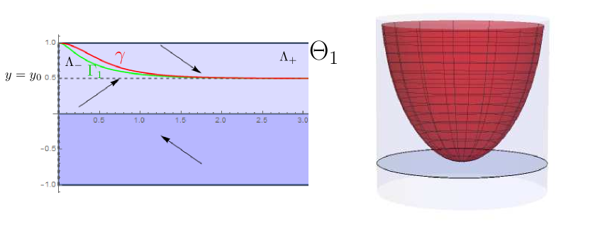
  Figure 1: Left: the phase plane $\Theta_{1}$, the regions $\Lambda_{+}$ and $\Lambda_{-}$, the curve $\Gamma_{1}$ in green and the orbit $\gamma_{+}$ in red. Right: an $\mathfrak{h}$-bowl in $\mathbb{H}^{2}\times\mathbb{R}$. The prescribed function is $\mathfrak{h}(y)=\sqrt{3}(y-0.25)$.

To finish, note that the case $\mathfrak{h}(-1)>0$, $y_{*}\leq 0$ is treated analogously; and the two remaining cases, $\mathfrak{h}(1)<0$, $y_{*}\geq 0$ and $\mathfrak{h}(-1)<0$, $y_{*}\leq 0$, can be reduced to the previous ones by changing the orientation. $\Box$

These $\mathfrak{h}$-surfaces will be called $\mathfrak{h}$-bowls, in analogy with the theory of self-translating solitons of the mean curvature flow (see [Bue1, Bue2, LiMa]) that we extend with the previous result. See Figure 1, right, for a graphic of an $\mathfrak{h}$-bowl in $\mathbb{H}^{2}\times\mathbb{R}$.

Secondly, we study the existence of catenoid-type rotational $\mathfrak{h}$-surfaces under appropiate conditions for the prescribed function $\mathfrak{h}$.

Proposition 3.2

Let $\mathfrak{h}$ be a $C^{1}$ function on $[-1,1]$, and suppose that $\mathfrak{h}\leq 0$ and $\mathfrak{h}(\pm 1)=0$. Then, there exists a one-parameter family of properly embedded, rotational $\mathfrak{h}$-surfaces in $\mathbb{H}^{2}\times\mathbb{R}$ of strictly negative extrinsic curvature at every point, and diffeomorphic to $\mathbb{S}^{1}\times\mathbb{R}$. Each example is a bi-graph over $\mathbb{H}^{2}-\mathbb{D}_{\mathbb{H}^{2}}(x_{0})$, where $\mathbb{D}_{\mathbb{H}^{2}}(x_{0})=\{x\in\mathbb{H}^{2}:|x|_{\mathbb{H}^{2}}<x_{0}\}$, for some $x_{0}>0$.

• Let $\Sigma(x_{0})$ be the rotational $\mathfrak{h}$-surface generated by the arc-length parametrized curve $\alpha(s)=(x(s),z(s))$ with the following initial conditions

  $$x(0)=x_{0},\;z(0)=0,\;\mathrm{and}\;z^{\prime}(0)=1,\ \mathrm{with}\ x_{0}>0.$$

  Then, the orbit $\gamma(s)=(x(s),y(s))$ of system (2.4) associated to $\alpha(s)$ passes through the point $(x_{0},0)$ at $s=0$. Moreover, $\gamma$ is contained in $\Theta_{1}$ around such a point, that is, $\varepsilon=1$.

  Observe that the curve $\Gamma_{1}$ given by (2.5) does not exist because of the assumption $\mathfrak{h}\leq 0$. Consequently, by item $4$ in Lemma 2.1 there are two monotonicity regions of $\Theta_{1}$ given by $\Lambda_{+}:=\{(x,y)\in\Theta_{1}:y>0\}$ and $\Lambda_{-}:=\{(x,y)\in\Theta_{1}:y<0\}$. Then, from (2.4) we know that $\gamma$ satisfies $x^{\prime}>0$ and $y^{\prime}>0$ in $\Lambda_{+}$, and $x^{\prime}<0$ and $y^{\prime}>0$ in $\Lambda_{-}$; see Figure 2, left.

  

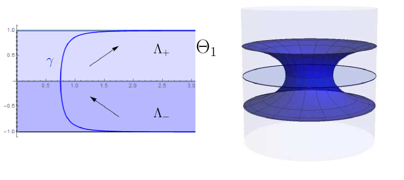
  Figure 2: Left: the phase plane $\Theta_{1}$, the monotonicity regions $\Lambda_{+}$ and $\Lambda_{-}$, and an orbit $\gamma$ in blue. Right: an $\mathfrak{h}$-catenoid in $\mathbb{H}^{2}\times\mathbb{R}$. The prescribed function is $\mathfrak{h}(y)=y^{2}-1$.

  Let us prove now that $\gamma$ must be a proper arc strictly contained in $\Theta_{1}$ satisfying $\gamma(s)\rightarrow(\infty,\pm 1)$ as $s\rightarrow\pm\infty$. First note that, the assumption $\mathfrak{h}\leq 0$ implies that given $y_{0}\in(-1,1)$, the equation $2\mathfrak{h}(y_{0})=\sqrt{1-y_{0}^{2}}$ has no solutions, so from Proposition 2.3 $\gamma$ cannot satisfy $\gamma(s)\rightarrow(\infty,y_{0})$ as $s\rightarrow\pm\infty$. Second, since $\mathfrak{h}\in C^{1}$ and $\mathfrak{h}(\pm 1)=0$, from the uniqueness of the Cauchy problem associated to (2.4), the curve $(s,\pm 1),\ s>0,$ is a solution to (2.4) which corresponds to a horizontal plane $\mathbb{H}^{2}\times\{t_{0}\},\ t_{0}\in\mathbb{R},$ endowed with $\pm\partial_{z}$ as unit normal, that is, $\gamma(s)$ cannot satisfy $\gamma(s_{0})=(x_{0},\pm 1)$ for some $s_{0}\in\mathbb{R}$. Finally, it remains to show that $\gamma(s)$ cannot converge to some $(x_{0},\pm 1),\ x_{0}>0,$ as $s\rightarrow\pm\infty$. Otherwise, there would exist $s_{0}\in\mathbb{R}$ such that for $|s|>|s_{0}|$, $x(s)$ is a monotonous function satisfying $x(s)\rightarrow x_{0}$ as $|s|\rightarrow\infty$. Thus, the mean value theorem ensures us that $x^{\prime}(s)=y(s)\rightarrow 0$, which is a contradiction with the fact that $y(s)\rightarrow\pm 1$.

Thus, $\Sigma(x_{0})$ is a bi-graph in $\mathbb{H}^{2}\times\mathbb{R}$ over $\Omega(x_{0}):=\mathbb{H}^{2}-\mathbb{D}_{\mathbb{H}^{2}}(x_{0})$, with the topology of $\mathbb{S}^{1}\times\mathbb{R}$. Indeed, $\Sigma(x_{0})=\Sigma_{1}\cup\Sigma_{2}$ where both $\Sigma_{i}$ are graphs over $\Omega(x_{0})$ with $\partial\Sigma_{i}=\partial\Omega(x_{0})$ and $\Sigma_{i}$ meets the horizontal plane $\mathbb{H}^{2}\times\{0\}$ in an orthogonal way along $\partial\Sigma_{i}$ (see Figure 2 right).

It remains to prove that the extrinsic curvature of $\Sigma(x_{0})$ is strictly negative. By (2.4) we get $y^{\prime}(s)>0$ for all $s$, so from (2.6) we derive $\kappa_{1}<0$ and $\kappa_{2}>0$ at every $p\in\Sigma$. $\Box$

This one-parameter family of rotational $\mathfrak{h}$-surfaces is a generalization of the usual minimal catenoids in $\mathbb{H}^{2}\times\mathbb{R}$, and this is the reason for calling them $\mathfrak{h}$-catenoids. As happens for the minimal catenoids, the $\mathfrak{h}$-catenoids are parametrized by their necksizes, i.e. the distance of their waists to the axis of rotation.

4 Classification of rotational $\mathfrak{h}$-surfaces with linear prescribed mean curvature

Our aim in this section is to classify the rotational examples of the following class of $\mathfrak{h}$-surfaces:

Definition 4.1

An oriented surface $\Sigma$ immersed in $\mathbb{H}^{2}\times\mathbb{R}$ is an $\mathfrak{h}_{\lambda}$-surface if its mean curvature function $H_{\Sigma}$ satisfies

$$H_{\Sigma}(p)=\mathfrak{h}_{\lambda}(\nu(p))=a\nu(p)+\lambda,\ \forall p\in\Sigma,\hskip 14.22636pta,\lambda\in\mathbb{R}.$$ (4.1)

Note that if $a=0$, then we are studying surfaces with constant mean curvature equal to $\lambda$. Also, if $\lambda=0$ the $\mathfrak{h}_{\lambda}$-surfaces are translating solitons of the mean curvature flow, see [Bue1, Bue2, LiMa]. Hence, we suppose that $a,\lambda$ are not null in order to avoid these cases. After a homothety in $\mathbb{H}^{2}\times\mathbb{R}$ we can suppose $a=1$ in Equation (4.1). Moreover, if $\Sigma$ is an $\mathfrak{h}_{\lambda}$-surface, then $\Sigma$ with its opposite orientation is an $\mathfrak{h}_{-\lambda}$-surface. Therefore, we will assume $\lambda>0$ without losing generality. In particular this implies that $\varepsilon\mathfrak{h}(0)>0$ if and only if $\varepsilon=1$, and consequently the equilibrium $e_{0}=(\arg\tanh(\frac{1}{2\varepsilon\mathfrak{h}(0)}),0)$ can only exist in $\Theta_{1}$. The CMC vertical cylinder generated by $e_{0}$ will be denoted by $C_{\lambda}$.

First, we announce two technical results that will be useful in the sequel. The first one was originally proved by López in [Lop] for surfaces in $\mathbb{R}^{3}$ whose mean curvature is given by Equation (4.1).

Lemma 4.2

There do not exist closed $\mathfrak{h}_{\lambda}$-surfaces in $\mathbb{H}^{2}\times\mathbb{R}$.

• Arguing by contradiction, suppose that $\Sigma$ is a closed $\mathfrak{h}_{\lambda}$-surface in $\mathbb{H}^{2}\times\mathbb{R}$. If $h:\Sigma\rightarrow\mathbb{R}$ denotes the height function of $\Sigma$, it is known that the Laplace-Beltrami operator $\Delta_{\Sigma}$ of $h$ is $\Delta_{\Sigma}h=2H_{\Sigma}\langle\eta,\partial_{z}\rangle$. Since $\Sigma$ is an $\mathfrak{h}_{\lambda}$-surface, we get

  $$\Delta_{\Sigma}h=2\langle\eta,\partial_{z}\rangle^{2}+2\lambda\langle\eta,\partial_{z}\rangle.$$

  We integrate this equation in $\Sigma$. By the divergence theorem and since $\partial\Sigma=\varnothing$, we have

  $$0=\int_{\Sigma}\langle\eta,\partial_{z}\rangle^{2}d\Sigma+\lambda\int_{\Sigma}\langle\eta,\partial_{z}\rangle d\Sigma.$$

  The second integral is zero by the divergence theorem, since the constant vector field $\partial_{z}$ has zero divergence. So, the first integral vanishes, that is, $\Sigma$ is contained in a cylindrical surface of the form $\beta\times\mathbb{R},\ \beta\subset\mathbb{H}^{2}$ being a curve, which contradicts that $\Sigma$ is compact. $\Box$

The second result forbids the existence of closed orbits in the phase plane of system (2.4) for some prescribed functions $\mathfrak{h}$. It follows from Bendixson-Dulac theorem, a classical result which appears in most textbooks on differential equations; see e.g. [ADL].

Theorem 4.3

Let $\mathfrak{h}$ be a $C^{1}$ function on $[-1,1]$ such that $\mathfrak{h}^{\prime}(y)\neq 0,\ \forall y\in(-1,1)$. Then, there do not exist closed orbits in $\Theta_{\varepsilon}$.

• Let us write system (2.4) as

  $$\left(\begin{array}[]{c}x\\ y\end{array}\right)^{\prime}=\left(\begin{array}[]{c}y\\ \displaystyle{\frac{1-y^{2}}{\tanh x}}-2\varepsilon\mathfrak{h}(y)\sqrt{1-y^{2}}\end{array}\right)=\left(\begin{array}[]{c}P(x,y)\\ Q(x,y)\end{array}\right),$$

  and define the function $\alpha:\Theta_{\varepsilon}\rightarrow\mathbb{R}$ and the vector field $V:\Theta_{\varepsilon}\rightarrow\Theta_{\varepsilon}$ as

  $$\alpha(x,y)=\frac{\sinh x}{\sqrt{1-y^{2}}},\hskip 14.22636ptV(x,y)=\alpha(x,y)(P(x,y),Q(x,y)).$$

  Arguing by contradiction, suppose that there exists some closed orbit $\overline{\gamma}$ in $\Theta_{\varepsilon}$ and name $\Omega$ to its inner region. A simple computation yields $\mathrm{div}V=(\alpha P)_{x}+(\alpha Q)_{y}=-2\varepsilon\mathfrak{h}^{\prime}(y)\sinh x$, which has constant sign since $x>0$ in $\Theta_{\varepsilon}$ and $\mathfrak{h}^{\prime}(y)\neq 0$. Therefore, the divergence theorem in $\Omega$ yields

  $$0\neq\int_{\Omega}\mathrm{div}V=\int_{\gamma}\langle V,\textbf{n}_{\gamma}\rangle=0,$$

  where $\textbf{n}_{\gamma}$ is the unit normal to the curve $\gamma$. Recall that the last integral vanishes since $V$ is everywhere tangent to $\gamma$. This contradiction proves the result. $\Box$

In particular, the prescribed function $\mathfrak{h}_{\lambda}(y)=y+\lambda,\ \lambda>0$ lies in the hypothesis of Theorem 4.3, hence the phase plane $\Theta_{\varepsilon}$ of system (2.4) for $\mathfrak{h}_{\lambda}$-surfaces does not have closed orbits.

Now, suppose that $\Sigma$ is a rotational $\mathfrak{h}_{\lambda}$-surface generated by an arc-length parametrized curve $\alpha(s)=(x(s),z(s))$. Then, (1.3) and (2.2) yields

$$2H_{\Sigma}=2(x^{\prime}+\lambda)=x^{\prime}z^{\prime\prime}-x^{\prime\prime}z^{\prime}+\frac{z^{\prime}}{\tanh x}.$$ (4.2)

Our first goal is to study the structure of the orbits around $e_{0}=(\arg\tanh(\frac{1}{2\lambda}),0)$. Recall that $e_{0}$ exists if and only if $\lambda>1/2$; otherwise, $\arg\tanh$ is not well defined. The linearized system of (2.4) at $e_{0}$ is given by

$${\left(\begin{matrix}0&1\\ 1-4\lambda^{2}&-2\end{matrix}\right)},$$ (4.3)

whose eigenvalues are

$${\mu_{1}=-1+\sqrt{2-4\lambda^{2}},\hskip 28.45274pt\text{and}\hskip 28.45274pt\mu_{2}=-1-\sqrt{2-4\lambda^{2}}}.$$

From standard theory of non-linear autonomous systems we derive:

Lemma 4.4

In the above conditions, we have:

• If $\displaystyle{\lambda>\frac{\sqrt{2}}{2}}$, then $\mu_{1}$ and $\mu_{2}$ are complex conjugate with negative real part. Thus, $e_{0}$ has an inward spiral structure, and every orbit close enough to $e_{0}$ converges asymptotically to it spiraling around infinitely many times.

• If $\displaystyle{\lambda=\frac{\sqrt{2}}{2}}$, then $\mu_{1}=\mu_{2}=-1$. Thus, $e_{0}$ is an asymptotically stable improper node, and every orbit close enough to $e_{0}$ converges asymptotically to it, maybe spiraling around a finite number of times.

• If $\displaystyle{0<\lambda<\frac{\sqrt{2}}{2}}$, then $\mu_{1}$ and $\mu_{2}$ are different and real. Thus, $e_{0}$ is an asymptotically stable node and has a sink structure, hence every orbit close enough to $e_{0}$ converges asymptotically to it directly, i.e. without spiraling around.

Now we stand in position to prove Theorem 1.2.

• Note that the behavior of the orbits in each phase plane $\Theta_{\varepsilon}$ depends on the curve $\Gamma_{\varepsilon}$ and the monotonicity regions generated by it. Consequently, we analyze three different cases for $\lambda$: $\lambda>\sqrt{5}/2$, $\lambda=\sqrt{5}/2$ and $0<\lambda<\sqrt{5}/2$.

  Case $\lambda>\sqrt{5}/2$

  Let us assume $\lambda>\sqrt{5}/2$. For $\varepsilon=1$, the curve $\Gamma_{1}$ given by (2.5) is a compact connected arc in $\Theta_{1}$ joining $(0,1)$ and $(0,-1)$, whereas for $\varepsilon=-1$, since $\mathfrak{h}$ is positive, the curve $\Gamma_{-1}$ does not exist in $\Theta_{-1}$. As a matter of fact, by item $4$ in Lemma 2.1 we know that there are four monotonicity regions in $\Theta_{1}$ which will be denoted by $\Lambda_{1},\dots,\Lambda_{4}$, and there are only two monotonicity regions in $\Theta_{-1}$ which will be denoted by $\Lambda_{+}$ and $\Lambda_{-}$. See Figure 3.

  

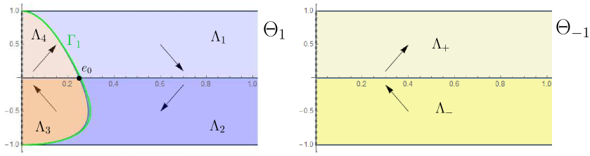
  Figure 3: The phase planes $\Theta_{1}$ and $\Theta_{-1}$ for $\lambda>\sqrt{5}/2$ with their monotonicity regions and the direction of the motion of the orbits at each of them.

Now, by using Corollary 2.5 it is clear that there exists a unique orbit $\gamma_{+}$ (resp. $\gamma_{-}$) in $\Theta_{1}$ with $(0,1)$ (resp. $(0,-1)$) as an endpoint.

On the one hand, let us study the behavior of $\gamma_{+}$. Firstly, we can suppose that such an orbit satisfies $\gamma_{+}(0)=(0,1)$ in $\Theta_{1}$, i.e., it generates an arc-length parametrized curve $\alpha_{+}(s)$ intersecting orthogonally the rotation axis with upwards oriented unit normal at $s=0$ . Because of the monotonicity properties, $\gamma_{+}(s)$ is strictly contained in the region $\Lambda_{1}$ for $s>0$ small enough. However, the orbit $\gamma_{+}$ cannot stay forever in $\Lambda_{1}$, otherwise $\gamma_{+}$ would be globally defined by a graph $y=f(x)$ such that

$$f(0)=1,\quad f^{\prime}(x)<0\;\;\forall x>0\quad\textrm{and}\quad\lim\limits_{x\rightarrow\infty}f(x)=c\in[0,1).$$

This contradicts Proposition 2.3 since $\lambda>\sqrt{5}/2$ and hence $2\mathfrak{h}_{\lambda}(y)=2(y+\lambda)>\sqrt{1-y^{2}}$. Thus, $\gamma_{+}(s)$ intersects the axis $y=0$ in an orthogonal way at a point $(x_{+},0)$ with $x_{+}>\arg\tanh\left(\frac{1}{2\lambda}\right)$ at some finite instant $s_{+}>0$.

On the other hand, for the orbit $\gamma_{-}$ we assume that $\gamma_{-}(0)=(0,-1)$ in $\Theta_{1}$, that is, it generates an arc-length parametrized curve $\alpha_{-}(s)$ intersecting orthogonally the axis of rotation with downwards oriented unit normal at $s=0$. By an analogous reasoning, we can assert that $\gamma_{-}(s)$ intersects $y=0$ orthogonally at $(x_{-},0)$ with $x_{-}>\arg\tanh\left(\frac{1}{2\lambda}\right)$ at some finite instant $s_{-}<0$.

Now, we prove that $x_{+}<x_{-}$ arguing by contradiction. First, see that if $x_{+}=x_{-}=\bar{x}$, by uniqueness of the Cauchy problem the orbits $\gamma_{+}$ and $\gamma_{-}$ could be smoothly glued together constructing a larger orbit $\bar{\gamma}$ which would be a compact arc joining the points $(0,1)$, $(\bar{x},0)$ and $(0,-1)$ and so the rotational $\mathfrak{h}_{\lambda}$-surface generated would be a rotational $\mathfrak{h}$-sphere, which is impossible because of Lemma 4.2. Additionally, if $x_{+}>x_{-}$, it would mean that $\gamma_{-}$ intersect the axis $y=0$ at the left-hand side of $\gamma_{+}$, and consequently the only possibility for $\gamma_{-}$ would be to enter the region $\Lambda_{1}$, later $\Lambda_{4}$ and after that $\Lambda_{3}$. In any case, $\gamma_{-}$ cannot converge to any point $(0,y),\ |y|<1$ in virtue of Lemma 2.4. Repeating this process, and since $\gamma_{-}$ cannot self-intersect nor converge to a closed orbit by Theorem 4.3, $\gamma_{-}$ finishes converging asymptotically to the equilibrium $e_{0}$ as $s\rightarrow-\infty$, spiriling around infinitely many times. This is a contradiction with the inward spiral structure of $e_{0}$, since this orbit would tend to escape from $e_{0}$ when $s$ increases. See Figure 4.

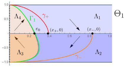
Figure 4: The phase plane $\Theta_{1}$ for $\lambda>\sqrt{5/2}$ with the configurarion of the orbits $\gamma_{+}$ and $\gamma_{-}$, plotted in red and orange, respectively, until they intersect the axis $y=0$.

Let us continue by analyzing the global behavior of both orbits. Firstly, when $\gamma_{+}$ passes through $(x_{+},0)$, it enters to $\Lambda_{2}$ but cannot intersect $\gamma_{-}$, so $\gamma_{+}$ has to enter to $\Lambda_{3}$. After that, due to the monotonicity properties and Lemma 2.4 we deduce that $\gamma_{+}$ has to enter to $\Lambda_{4}$ and intersect $\Gamma_{1}$. Since $\gamma_{+}$ cannot self-intersect nor converge to a limit closed orbit in $\Theta_{1}$ in virtue of Theorem 4.3, the only possibility for $\gamma_{+}$ is to repeat this behavior and eventually converge asymptotically to the equilibrium $e_{0}$ (see the plot of $\gamma_{+}$ in Figure 5 top-left). Furthermore, since $\lambda>\sqrt{2}/2$, $\gamma_{+}$ spirals around $e_{0}$ infinitely many times.

In this way, $\gamma_{+}$ generates the curve $\alpha_{+}(s)=(x_{+}(s),z_{+}(s))$ satisfying: the $x_{+}(s)-$coordinate is bounded by the value $x_{+}$ and converges to $\arg\tanh\left(\frac{1}{2\lambda}\right)$; and the $z_{+}(s)$-coordinate is strictly increasing since $\gamma_{+}\subset\Theta_{1}$, hence $z^{\prime}_{+}(s)>0$. Then, $\alpha_{+}(s)$ is an embedded curve that converges to the line $x=\arg\tanh\left(\frac{1}{2\lambda}\right)$ intersecting it infinitely many times. Therefore, after rotating such a curve around the rotation axis, we derive that the generated surface $\Sigma_{+}$ is a properly embedded, simply connected $\mathfrak{h}_{\lambda}$-surface that converges to the CMC cylinder $C_{\lambda}$ intersecting it infinitely many times. See $\Sigma_{+}$ in Figure 5 top-right.

Now we focus on $\gamma_{-}$, which intersects the axis $y=0$ at the point $\gamma_{-}(s_{-})=(x_{-},0)$ at some finite instant $s_{-}<0$. So, when the parameter $s<s_{-}$ decreases, $\gamma_{-}$ enters to $\Lambda_{1}$. Bearing in mind that $\gamma_{+}$ and $\gamma_{-}$ cannot intersect, from the monotonicity properties we deduce that $\gamma_{-}$ has as endpoint $\gamma_{-}(s_{1})=(x_{1},1)$ with $0<x_{1}<x_{-}$ and $s_{1}<s_{-}$. Then, $\gamma_{-}$ generates the curve $\alpha_{-}(s)=(x_{-}(s),z_{-}(s))$ satisfying that: $x_{-}(s_{1})=x_{1}$ and $x_{-}^{\prime}(s_{1})=1$, so from (4.2) we get $z_{-}^{\prime\prime}(s_{1})>0$, i.e., the height of $\alpha_{-}$ reaches a minimum at $s_{1}$. If we name $\Sigma_{-}$ to the $\mathfrak{h}_{\lambda}$-surface associated to $\gamma_{-}$ and generated by rotating $\alpha_{-}(s)$, the image of the points $\alpha_{-}(s_{1})$ under such rotation corresponds to points on the boundary of $\Sigma_{-}$ having unit normal $\partial_{z}$.

Therefore, for $s<s_{1}$, $s$ close enough to $s_{1}$, the height function $z_{-}(s)$ of $\alpha_{-}(s)$ is decreasing, i.e. $z_{-}^{\prime}(s)<0$. Consequently, $\alpha_{-}(s)$ for $s<s_{1}$ close enough to $s_{1}$ generates an orbit in $\Theta_{-1}$ (since $\varepsilon=\mathrm{sign}(z^{\prime}_{-})=-1$), which will be named $\gamma_{-}$ for saving notation. Hence, the orbit $\gamma_{-}(s)$ continues from $\Theta_{1}$ to $\Theta_{-1}$ as $s$ decreases from $s=s_{1}$. At this point, the continuation of $\gamma_{-}$ between the phase planes $\Theta_{\pm 1}$ has to be understood as the extension of $\Sigma_{-}$ by solving the Cauchy problem for rotational vertical $\mathfrak{h}_{\lambda}$-graphs having the same vertical unit normal.

Hence, $\gamma_{-}(s)$ belongs to $\Theta_{-1}$ for $s<s_{1}$ close enough to $s_{1}$ and lies in the region $\Lambda_{+}$. Once again, by monotonicity, $\gamma_{-}$ must intersect the axis $y=0$ orthogonally and enter to $\Lambda_{-}$. As $\gamma_{-}$ cannot stay forever in $\Lambda_{-}$ with $x_{-}(s)\rightarrow\infty$ for $s\rightarrow-\infty$, we derive that there exists $s_{2}<s_{1}$ such that $\gamma_{-}(s_{2})=(x_{2},-1)$ (see the plot of $\gamma_{-}$ in Figure 5 left). Repeating this process indefinitely, we construct a complete, arc-length parametrized curve $\alpha_{-}(s)$ with infinitely many self-intersections, whose height function increases and decreases until reaching the rotation axis. Hence, the generated rotational $\mathfrak{h}_{\lambda}$-surface $\Sigma_{-}$ is properly immersed (with self-intersections) and simply connected. See Figure 5, bottom right.

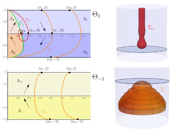
Figure 5: Left: the phase planes $\Theta_{1}$ and $\Theta_{-1}$ for $\lambda>\sqrt{5}/2$ and the orbits $\gamma_{+}$ and $\gamma_{-}$, plotted in red and orange, respectively. Right: the corresponding rotational $\mathfrak{h}_{\lambda}$-surfaces $\Sigma_{+}$ and $\Sigma_{-}$.

Case $\lambda=\sqrt{5}/2$

Assume that $\lambda=\sqrt{5}/2$. For $\varepsilon=1$, $\Gamma_{1}$ is formed by two connected arcs $\Gamma_{1}^{\pm}$, each of them having the point $(0,\pm 1)$ as endpoint respectively, and both having the line $y=-2/\sqrt{5}$ as an asymptote. From item $4$ in Lemma 2.1 we find five monotonicity regions in the phase plane $\Theta_{1}$ denoted by $\Lambda_{1},\dots,\Lambda_{5}$ (see Figure 6 left). For $\varepsilon=-1$, the phase plane $\Theta_{-1}$ is exactly the same that in the previous case $\lambda>\sqrt{5}/2$.

From Corollary 2.5 we can assert that there exists a unique orbit $\gamma_{+}$ (resp. $\gamma_{-}$) in $\Theta_{1}$ with $(0,1)$ (resp. $(0,-1)$) as an endpoint.

Regarding the orbit $\gamma_{+}$, it converges to $e_{0}=(\mathrm{argtanh}\frac{1}{\sqrt{5}},0)$ as $s\rightarrow\infty$ spiraling around it infinitely many times in the same fashion as the orbit $\gamma_{+}$ studied in the previous case $\lambda>\sqrt{5}/2$, see Figure 6 left. Consequently, its corresponding $\mathfrak{h}_{\lambda}$-surface $\Sigma_{+}$ has the same behavior as the one shown in Figure 5, top right.

Now, consider the orbit $\gamma_{-}$ such that $\gamma_{-}(0)=(0,-1)$. It is clear that $\gamma_{-}(s)$ is totally contained in $\Lambda_{3}$ and when the parameter $s$ tends to $-\infty$, the orbit $\gamma_{-}(s)$ converges to the line $y=-2/\sqrt{5}$. Note that $\gamma_{-}(s)$ cannot converge to other line $y=y_{0},\ y_{0}\in(-1,-2/\sqrt{5})$ in virtue of Proposition 2.3 (see the plot of $\gamma_{-}$ in Figure 6 left). Therefore, the generated $\mathfrak{h}_{\lambda}$-surface $\Sigma_{-}$ is an entire, strictly convex graph whose angle function tends to the value $-2/\sqrt{5}$. See Figure 6 right.

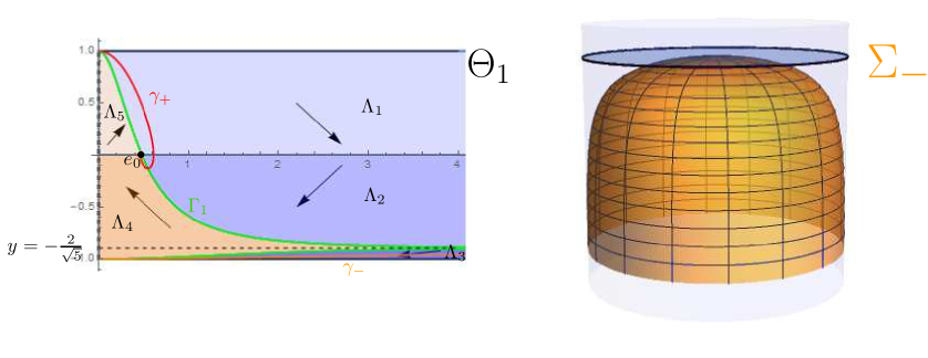
Figure 6: Left: the phase plane $\Theta_{1}$ for $\lambda=\sqrt{5}/2$ and the orbits $\gamma_{+}$ and $\gamma_{-}$, plotted in red and orange, respectively. Right: the corresponding rotational $\mathfrak{h}_{\lambda}$-surface $\Sigma_{-}$.

Case $\lambda<\sqrt{5}/2$

We begin by analyzing the behavior of $\Gamma_{\varepsilon}$ in $\Theta_{\varepsilon}$. Recall that the equilibrium $e_{0}$ exists in $\Theta_{1}$ if and only if $\lambda>1/2$. Additionally, we define the candidates of asymptotes for $\Gamma_{\epsilon}$ as:

$$y_{0}^{+}:=\frac{1}{5}(-4\lambda+\sqrt{5-4\lambda^{2}}),\quad\textrm{and}\quad y_{0}^{-}:=\frac{1}{5}(-4\lambda-\sqrt{5-4\lambda^{2}}).$$

Let us distinguish further cases of $\lambda$:

• If $\lambda>1$, then $\Gamma_{1}$ is a disconnected arc having two connected components $\Gamma_{1}^{+}$ and $\Gamma_{1}^{-}$, with $\Gamma_{+}$ (resp. $\Gamma_{-}$) having the point $(0,1)$ (resp. $(0,-1)$) as an endpoint and the line $y=y_{0}^{+}$ (resp. $y=y_{0}^{-}$) as asymptote; see Figure 7. The curve $\Gamma_{-1}$ does not exist in $\Theta_{-1}$ as in the previous cases.

  

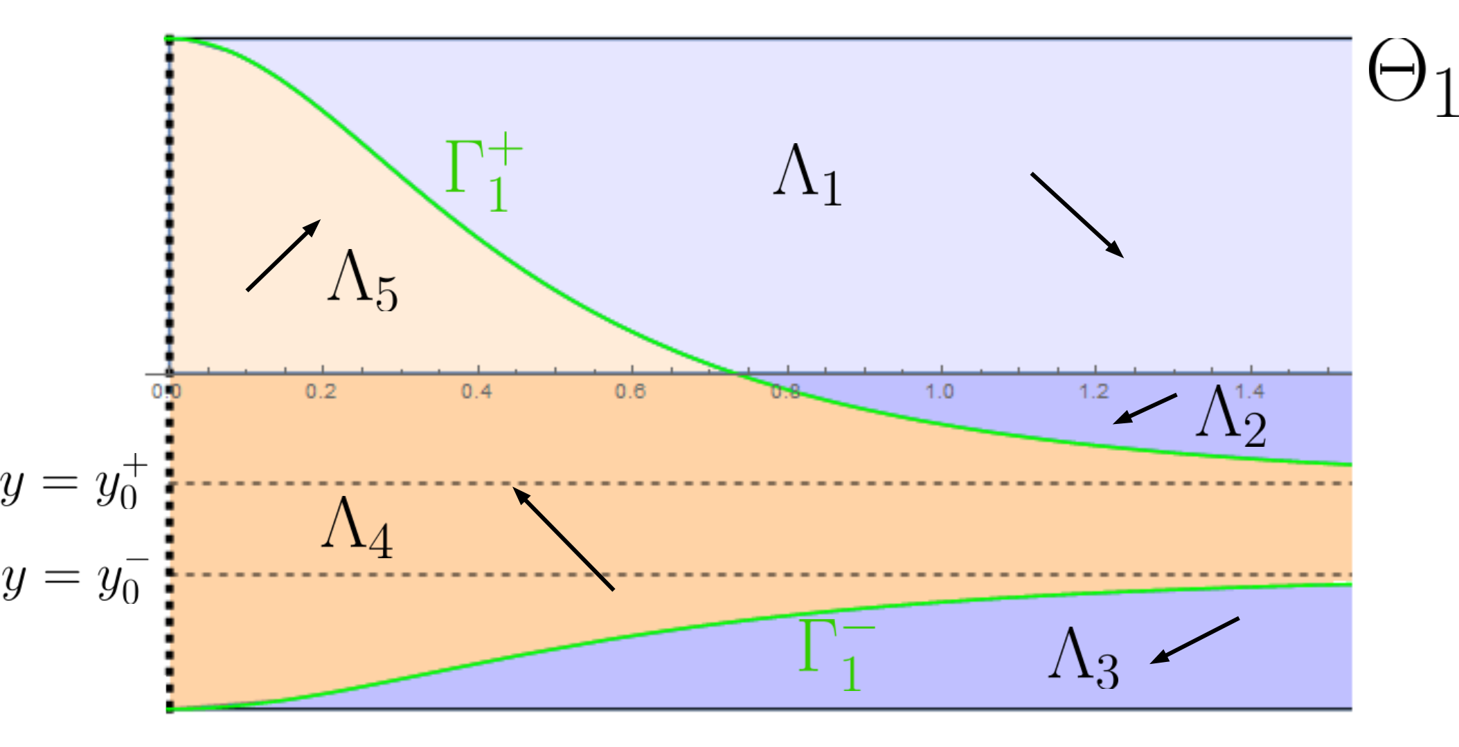
  Figure 7: The phase plane $\Theta_{1}$ for some $\lambda\in(1,\sqrt{5}/2)$.

• If $\lambda=1$, then $\Gamma_{1}$ is a connected arc having $(0,1)$ as endpoint and the line $y=y_{0}^{+}=-3/5$ as asymptote. The line $y=y_{0}^{-}=-1$ does not appear. The curve $\Gamma_{-1}$ does not exist in $\Theta_{-1}$.

• If $\lambda<1$, then $\Gamma_{1}$ is a connected arc having $(0,1)$ as endpoint and the line $y=y_{0}^{+}$ as asymptote. Moreover, $y_{0}^{+}\geq 0$ if and only if $\lambda\leq 1/2$. The curve $\Gamma_{-1}$ is a connected arc having $(0,-1)$ as endpoint and the line $y=y_{0}^{-}$ as an asymptote; see Figure 8.

  

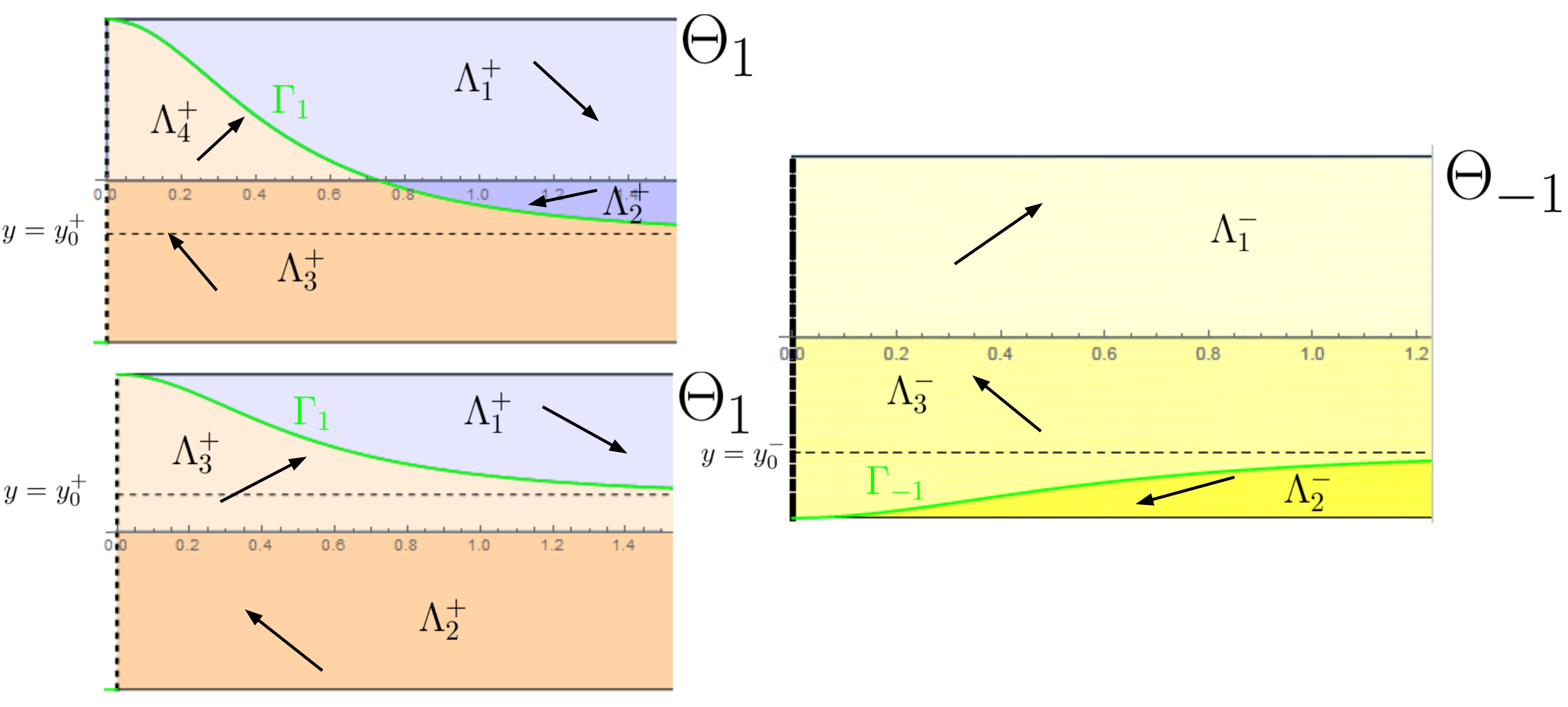
  Figure 8: Top left: the phase plane $\Theta_{1}$ for $\lambda>1/2$. Bottom left: the phase plane $\Theta_{1}$ for $\lambda\leq 1/2$. Right: the phase plane $\Theta_{-1}$ for $\lambda<1$.

Now, we study the behavior of the orbits. Once again, the existence of the orbit $\gamma_{+}(s)$ in $\Theta_{1}$ such that $\gamma(0)=(0,1)$ follows from Corollary 2.5. Then, if we suppose that $\lambda\leq 1/2$, $\gamma_{+}(s)$ stays in $\Lambda_{1}^{+}$ as it converges to the line $y=y_{0}^{+}$, and so $\Sigma_{+}$ is an entire, strictly convex graph. Otherwise, i.e., if $\lambda>1/2$, the equilibrium $e_{0}$ exists. Since no closed orbit exists in virtue of Theorem 4.3, $\gamma_{+}$ converges to $e_{0}$ as $s\rightarrow\infty$, and its behavior is detailed in Lemma 4.4. Consequently, $\Sigma_{+}$ is a properly embedded, simply connected $\mathfrak{h}_{\lambda}$-surface and:

• If $\displaystyle{\lambda>\frac{\sqrt{2}}{2}}$, $\Sigma_{+}$ intersects $C_{\lambda}$ infinitely many times.

• If $\displaystyle{\lambda=\frac{\sqrt{2}}{2}}$, $\Sigma_{+}$ intersects $C_{\lambda}$ a finite number of times.

• If $\displaystyle{\lambda<\frac{\sqrt{2}}{2}}$, $\Sigma_{+}$ is a strictly convex graph contained in the solid cylinder bounded by $C_{\lambda}$ and converging asymptotically to it.

For the study of the orbit $\gamma_{-}(s)$ such that $\gamma_{-}(0)=(0,-1)$ we have to distinguish between the cases $\lambda>1,\ \lambda=1,\ \lambda<1$. This discussion will deeply influence the outcome of Corollary 2.5:

• If $\lambda>1$, then $\mathfrak{h}_{\lambda}(-1)>0$ and $\gamma_{-}(s)$ lies in $\Theta_{1}$.

• If $\lambda=1$, then $\mathfrak{h}_{\lambda}(-1)=0$ and $\gamma_{-}(s)$ does not exist in either $\Theta_{1}$ or $\Theta_{-1}$.

• If $\lambda<1$, then $\mathfrak{h}_{\lambda}(-1)<0$ and $\gamma_{-}(s)$ lies in $\Theta_{-1}$.

If $\lambda=1$, horizontal minimal planes downwards oriented are $\mathfrak{h}_{1}$-surfaces. Consequently, the uniqueness of the Cauchy problem of (2.4) extends to the line $y=-1$ and so no orbit can have and endpoint at this line.

If $\lambda\neq 1$, by monotonicity and Proposition 2.3, the only possibility for $\gamma_{-}(s)$ is to converge to the line $y=y_{0}^{-}$, and so $\Sigma_{-}$ is a downwards oriented, strictly convex, entire graph. For $\lambda>1$, the height of $\Sigma_{-}$ tends to minus infinity; for $\lambda<1$, the height of $\Sigma_{-}$ tends to infinity.

This concludes the classification of the rotational $\mathfrak{h}_{\lambda}$-surfaces that intersect the axis of rotation. $\Box$

To finish, we prove Theorem 1.3.

• First, the equilibrium $e_{0}=(\mathrm{argtanh}\frac{1}{2\lambda},0)$ exists if and only if $\lambda>\frac{1}{2}$. This equilibrium generates the cylinder $C_{\lambda}$ with CMC equal to $\lambda$ and vertical rulings. For the remaining $\mathfrak{h}_{\lambda}$-surfaces, we distinguish again three cases depending on $\lambda$. Take into account that the structure of the phase planes $\Theta_{1}$ and $\Theta_{-1}$ has been just studied in the previous proof. See Figure 3 for $\lambda>\sqrt{5}/2$, Figure 6 for $\lambda=\sqrt{5}/2$ and Figures 7 and 8 for $\lambda<\sqrt{5}/2$.

  Case $\lambda>\sqrt{5}/2$

  Let us take $x_{0}>\arg\tanh(\frac{1}{2\lambda})$ and let $\gamma(s)$ be the orbit in $\Theta_{1}$ passing through the point $(x_{0},0)$ at the instant $s=0$. For $s<0$, $\gamma$ has as endpoint some $(x_{1},1),\ x_{1}>0$ (if $x_{1}=0$, $\gamma=\gamma_{+}$), and for $s>0$ either converges to $e_{0}$ as $s\rightarrow\infty$ or has another endpoint of the form $(x_{2},-1),\ x_{2}>0$ (again, if $x_{2}=0$, $\gamma=\gamma_{-}$). In the second case, the orbit $\gamma$ continues in $\Theta_{-1}$ as a compact arc and then goes again in $\Theta_{1}$; see Figure 9, left. After a finite number of iterations, the orbit $\gamma$ eventually converges to $e_{0}$ spiraling around it infinitely many times.

  

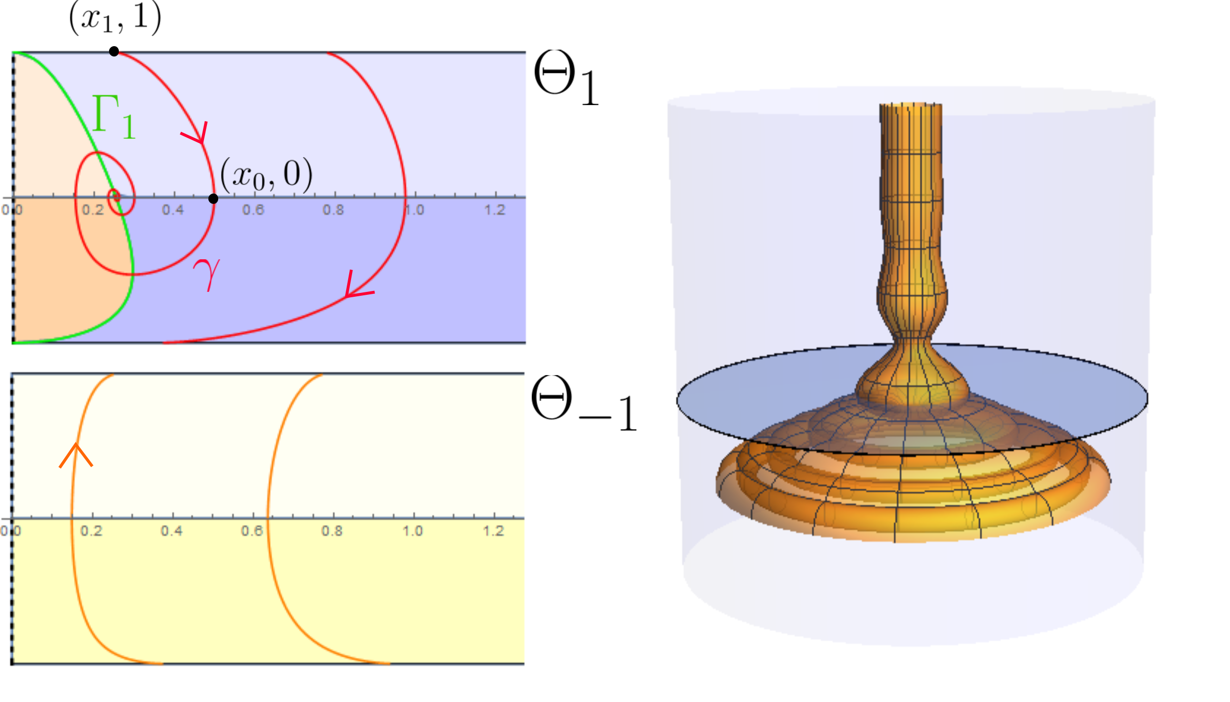
  Figure 9: Left: the phase planes $\Theta_{1}$ and $\Theta_{-1}$ for $\lambda>\sqrt{5}/2$ and an orbit $\gamma$. Right: the rotational $\mathfrak{h}_{\lambda}$-surface corresponding to $\gamma$.

This configuration ensures us that the $\mathfrak{h}_{\lambda}$-surface generated by $\gamma$ is properly immersed, non-embedded, and diffeomorphic to $\mathbb{S}^{1}\times\mathbb{R}$. One end converges to $C_{\lambda}$ intersecting it infinitely many times, and the other end has unbounded distance to the axis of rotation, looping and self-intersecting infinitely many times (see Figure 9, right).

Case $\lambda=\sqrt{5}/2$

Firstly, let us fix some $x_{0}>\arg\tanh(\frac{1}{\sqrt{5}})$ and consider the orbit $\gamma_{1}(s)$ passing through $(x_{0},0)$ at $s=0$. For $s<0$, $\gamma_{1}(s)$ is contained in $\Lambda_{1}$, so it satisfies $\gamma_{1}(s_{1})=(x_{1},1)$ as endpoint for some $s_{1}<0$. Hence, for $s<s_{1}$, $\gamma_{1}(s)$ lies in $\Theta_{-1}$ and is a compact arc whose other endpoint is located at some $\gamma_{1}(s_{2})=(x_{2},-1)$. Finally, for $s<s_{2}$, $\gamma_{1}(s)$ lies in the monotonicity region $\Lambda_{3}$ in $\Theta_{1}$ and stays there as it converges to the line $y=-2/\sqrt{5}$ as $s\rightarrow-\infty$; see Figure 10, top left, the red orbit.

For $s>0$, $\gamma_{1}(s)$ enters to $\Lambda_{2}$, then goes inside $\Lambda_{4}$ and intersects $y=0$ for the second time in some $(\widehat{x}_{0},0)$ with $\widehat{x}_{0}>0$. It is clear that when $x_{0}$ increases, then $\widehat{x}_{0}$ decreases and so $\widehat{x}_{0}\rightarrow x_{\infty}\geq 0$ as $x_{0}\rightarrow\infty$. Also, note that $\gamma_{1}(s)$ stays always above the line $y=-2/\sqrt{5}$ since the minimum of its $y(s)$-coordinate is at the intersection of $\gamma_{1}(s)$ with $\Gamma_{1}$. In this setting, we claim that $x_{\infty}>0$.

Arguing by contradiction, suppose that $x_{\infty}=0$ and consider an orbit $\sigma(s)$ such that $\sigma(0)$ lies in $\Lambda_{4}$ and is located below the line $y=-2/\sqrt{5}$. Then, for $s>0$ in virtue of Proposition 2.4 and by monotonicity, $\sigma(s)$ has to reach the axis $y=0$ at a point $(\widehat{r}_{1},0)$ for some finite instant. Due to the definition of $x_{\infty}$ and the assumption $x_{\infty}=0$, there exists $r>e_{0}$ and an orbit $\gamma$ such that $\gamma(0)=(r,0)$ and $\gamma(s_{1})=(\widehat{r},0)$ with $0<\widehat{r}<\widehat{r}_{1}$, for some $s_{1}>0$. Hence, $\sigma$ and $\gamma$ intersect each other, which is a contradiction with the uniqueness of the Cauchy problem.

Secondly, let be $r_{0}>0$ and take $\gamma_{2}(s)$ the orbit such that $\gamma_{2}(0)=(r_{0},-\sqrt{2}/5)$. For $s<0$, $\gamma_{2}(s)$ lies in $\Lambda_{4}$, intersects the curve $\Gamma_{1}^{-}$, enters $\Lambda_{3}$ and converges to the line $y=-2/\sqrt{5}$. For $s>0$, $\gamma_{2}(s)$ lies in $\Lambda_{4}$ until intersecting $y=0$ at some $(\widetilde{r_{0}},0)$. Moreover, as $r_{0}$ increases $\widetilde{r_{0}}$ also increases, and so $\widetilde{r_{0}}\rightarrow r_{\infty}$ as $r_{0}\rightarrow\infty$. In particular, $r_{\infty}\leq x_{\infty}$. For $s\rightarrow\infty$, $\gamma_{2}(s)$ converges asymptotically to $e_{0}$, spiraling around it infinitely many times; see Figure 10, top left, the blue orbit.

Finally, take some $\xi_{0}\in[r_{\infty},x_{\infty}]$ and let $\gamma_{3}(s)$ be the orbit such that $\gamma_{3}(0)=(\xi_{0},0)$. For $s>0$ it is clear that $\gamma_{3}(s)$ converges asymptotically to $e_{0}$, spiraling around it infinitely many times. Because of how $r_{\infty}$ and $x_{\infty}$ have been defined, for $s<0$ the orbit $\gamma_{3}(s)$ cannot intersect $\Gamma_{1}^{-}$ nor intersect $y=-2/\sqrt{5}$. Thus, the only possibility for $\gamma_{3}(s)$ is to converge to the line $y=-2/\sqrt{5}$ with strictly decreasing $y(s)$-coordinate; see Figure 10, top left, the purple orbit.

Thus, each orbit $\gamma_{i},\ i=1,2,3$ generates a properly immersed $\mathfrak{h}_{\lambda}$-surface $\Sigma_{i}$, diffeomorphic to $\mathbb{S}^{1}\times\mathbb{R}$, with one end converging asymptotically to the CMC cylinder $C_{\lambda}$ and the other being a graph outside a compact set. Moreover, $\Sigma_{1}$ is non-embedded, while $\Sigma_{2}$ and $\Sigma_{3}$ have monotonous height and in particular are embedded; see Figure 10, bottom.

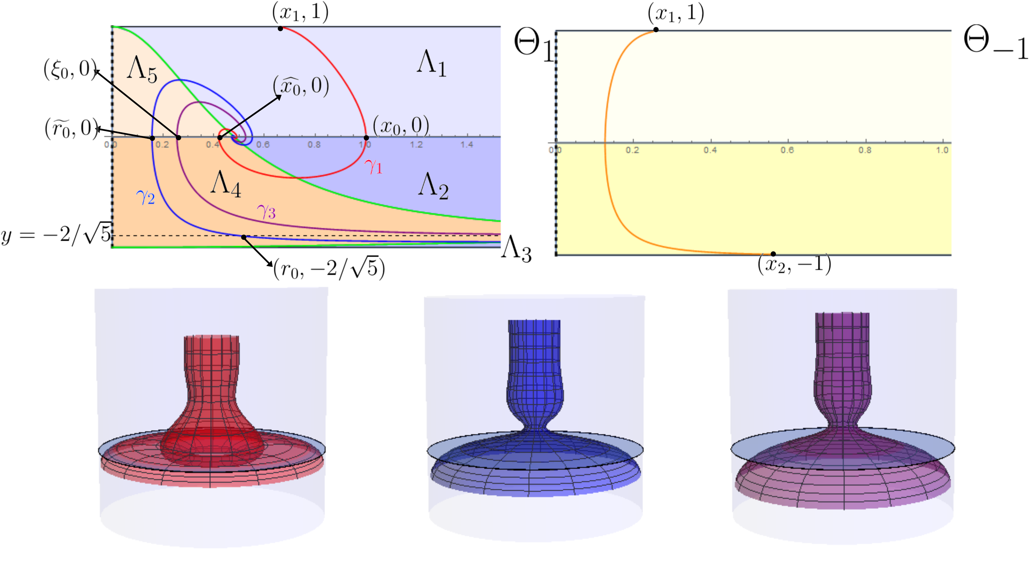
Figure 10: Top: the phase planes $\Theta_{1}$ and $\Theta_{-1}$ for $\lambda=\sqrt{5}/2$ and the three types of orbits $\gamma_{1}$, $\gamma_{2}$ and $\gamma_{3}$. Bottom: the three corresponding types of rotational $\mathfrak{h}_{\lambda}$-surfaces.

Case $\lambda<\sqrt{5}/2$

In this final case, we also distinguish between values of $\lambda$. Note that the equilibrium $e_{0}=(\arg\tanh(\frac{1}{2\lambda}),0)$ exists if and only if $\lambda>1/2$. Again, we define

$$y_{0}^{+}:=\frac{1}{5}(-4\lambda+\sqrt{5-4\lambda^{2}}),\quad\textrm{and}\quad y_{0}^{-}:=\frac{1}{5}(-4\lambda-\sqrt{5-4\lambda^{2}}).$$

• Case $1\leq\lambda<\sqrt{5}/2$. The structure of the phase plane $\Theta_{1}$ (resp. $\Theta_{-1}$) is the same as the one in Figure 7 (resp. Figure 3, right). Recall that $y_{0}^{-}=-1$ in $\Theta_{1}$ for $\lambda=1$ and there are only four monotonicity regions. The same reasoning as in the case $\lambda=\sqrt{5}/2$ ensures us that we can construct three types of orbits (see Figure 10) and also the points $x_{\infty}$ and $r_{\infty}$:

  • $\gamma_{1}(s)$ such that $\gamma_{1}(0)=(x_{0},0)$ with $x_{0}>\arg\tanh(\frac{1}{2\lambda})$ and $\gamma_{1}(s)\rightarrow e_{0}$ as $s\rightarrow\infty$.

  • $\gamma_{2}(s)$ such that $\gamma_{2}(0)=(r_{0},y_{0}^{+})$ with $r_{0}>0$, $\gamma_{2}(s)\rightarrow e_{0}$ as $s\rightarrow\infty$ and $\gamma_{2}(s)\rightarrow y_{0}^{-}$ as $s\rightarrow-\infty$.

  • $\gamma_{3}(s)$ such that $\gamma_{3}(0)=(\xi_{0},0)$ with $\xi_{0}\in[r_{\infty},x_{\infty}]$, $\gamma_{3}(s)\rightarrow e_{0}$ as $s\rightarrow\infty$ and $\gamma_{3}(s)\rightarrow y_{0}^{+}$ as $s\rightarrow-\infty$.

  Again, each orbit $\gamma_{i},\ i=1,2,3$ generates a properly immersed $\mathfrak{h}_{\lambda}$-surface $\Sigma_{i}$ that is diffeomorphic to $\mathbb{S}^{1}\times\mathbb{R}$, with one end converging asymptotically to the CMC cylinder $C_{\lambda}$ and the other being a graph outside a compact set. Moreover, $\Sigma_{1}$ self-intersects, while $\Sigma_{2}$ and $\Sigma_{3}$ have monotonous height and in particular are embedded.

• Case $1/2<\lambda<1$. In this case, the structure of $\Theta_{1}$ and $\Theta_{-1}$ is shown in Figure 8 top left and right respectively. There are also three kind of orbits $\gamma_{1}(s),\gamma_{2}(s),\gamma_{3}(s)$ in $\Theta_{1}$, and $\gamma_{1}(s)$ and $\gamma_{3}(s)$ behave as shown in Figure 10. The only difference here is that the orbit $\gamma_{2}(s)$ intersects the line $y=-1$ at a finite point as $s$ decreases. Then, $\gamma_{2}(s)$ enters to $\Theta_{-1}$ and converges to the line $y=y_{0}^{-}$ as $s\rightarrow-\infty$.

  The corresponding $\mathfrak{h}_{\lambda}$-surfaces are also similar to the ones constructed in the previous case.

• Case $\lambda\leq 1/2$. In this case, the structure of $\Theta_{1}$ and $\Theta_{-1}$ is shown in Figure 8 bottom left and right respectively. In particular, no equilibrium point exists and the behavior of the orbits is different from the previous cases.

  

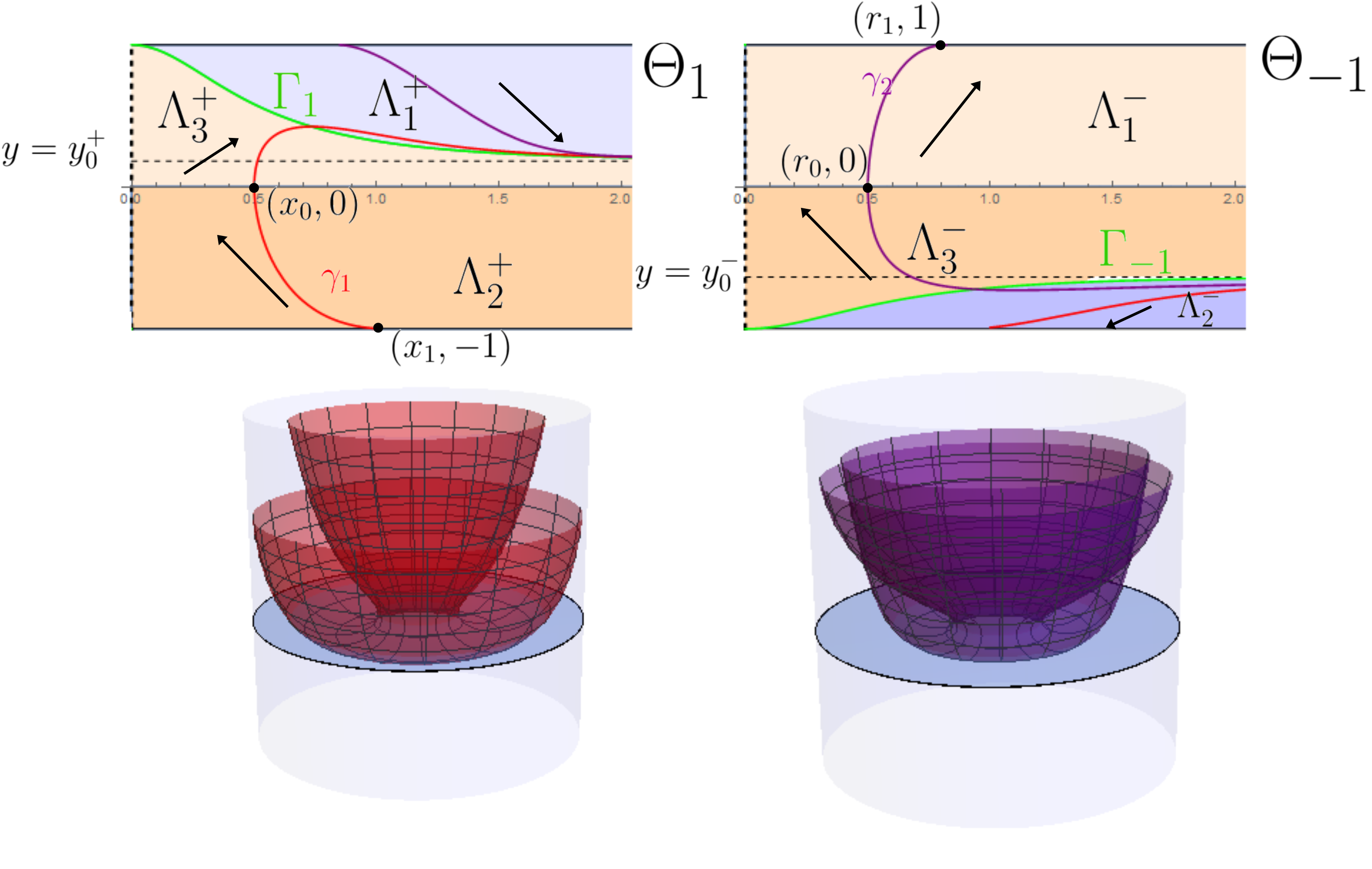
  Figure 11: Top: the phase planes $\Theta_{1}$ and $\Theta_{-1}$ for $\lambda=1/3$. Bottom: the two corresponding $\mathfrak{h}_{\lambda}$-surfaces for $\lambda=1/3$.

  First, let be $x_{0}>0$ and $\gamma_{1}(s)$ the orbit in $\Theta_{1}$ such that $\gamma_{1}(0)=(x_{0},0)$. For $s>0$, $\gamma_{1}(s)$ enters to $\Lambda_{3}^{+}$, intersects $\Gamma_{1}$ and then lies in $\Lambda_{1}^{+}$ converging to the line $y=y_{0}^{+}$. For $s<0$, the orbit $\gamma_{1}(s)$ lies in $\Lambda_{2}^{+}$ and has some $\gamma_{1}(s_{0})=(x_{1},-1)$ as endpoint. Thus, $\gamma_{1}(s)$ for $s<s_{0}$ lies in $\Lambda_{2}^{-}$ and stays there converging to the line $y=y_{0}^{-}$ as $s\rightarrow-\infty$. See Figure 11, the orbit in red.

  Lastly, let be $r_{0}>0$ and $\gamma_{2}(s)$ the orbit in $\Theta_{-1}$ such that $\gamma_{2}(0)=(r_{0},0)$. For $s<0$, $\gamma_{2}(s)$ enters the region $\Lambda_{3}^{-}$ and ends up converging to the line $y=y_{0}^{-}$ as $s\rightarrow-\infty$. For $s>0$, $\gamma(s)$ enters the region $\Lambda_{1}^{-}$ and has as endpoint some $\gamma_{2}(s_{0})=(r_{1},1)$. Then, $\gamma_{2}(s)$ for $s>s_{0}$ lies in $\Lambda_{1}^{+}$ and stays there as it converges to the line $y=y_{0}^{+}$ as $s\rightarrow\infty$. See Figure 11, the orbit in purple.

  Again, we have two distinct $\mathfrak{h}_{\lambda}$-surfaces $\Sigma_{1}$ and $\Sigma_{2}$ generated by the orbits $\gamma_{1}$ and $\gamma_{2}$. Each $\Sigma_{i}$ is properly immersed and diffeomorphic to $\mathbb{S}^{1}\times\mathbb{R}$, and both ends are graphs outside compact sets. Moreover, $\Sigma_{1}$ is embedded, while $\Sigma_{2}$ self intersects; see Figure 11, bottom.

$\Box$

References

- [AbRo] U. Abresch, H. Rosenberg, A Hopf differential for constant mean curvature surfaces in and , Acta Math. 193 (2004), 141–174.
- [Ale] A.D. Alexandrov, Uniqueness theorems for surfaces in the large, I, Vestnik Leningrad Univ. 11 (1956), 5–17. (English translation): Amer. Math. Soc. Transl. 21 (1962), 341–354.
- [ADL] J. C. Artés, F. Dumortier, J. Llibre. Qualitative theory of planar differential systems. Universitext. Springer-Verlag, Berlin, 2006.
- [BCMR] V. Bayle, A. Cañete, F. Morgan, C. Rosales, On the isoperimetric problem in Euclidean space with density, Calc. Var. Partial Diff. Equations 31 (2008), 27–46.
- [Bue1] A. Bueno, Translating solitons of the mean curvature flow in the space , J. Geom. 109 (2018).
- [Bue2] A. Bueno, Uniqueness of the translating bowl in , J. Geom., 111 (2020).
- [Bue3] A. Bueno, The Björling problem for prescribed mean curvature surfaces in , Ann. Global. Anal. Geom., 56 (2019), 87-96.
- [Bue4] A. Bueno, Half-space theorems for properly immersed surfaces in with prescribed mean curvature, Ann. Mat. Pura. Appl., 199 (2020), 425–444.
- [Bue5] A. Bueno, A Delaunay-type classification result for prescribed mean curvature surfaces in , preprint, arxiv:1807.10040.
- [Bue6] A. Bueno, Properly embedded surfaces with prescribed mean curvature in , Ann. Global. Anal. Geom., (2020), to appear. DOI:https://doi.org/10.1007/s10455-020-09741-6.
- [BGM1] A. Bueno, J.A. Gálvez, P. Mira, The global geometry of surfaces with prescribed mean curvature in , Trans. Amer. Math. Soc. 373 (2020), 4437-4467.
- [BGM2] A. Bueno, J.A. Gálvez, P. Mira, Rotational hypersurfaces of prescribed mean curvature, J. Differential Equations 268 (2020), 2394–2413.
- [BuOr] A. Bueno, I. Ortiz, Invariant hypersurfaces with linear prescribed mean curvature, J. Math. Anal. Appl., 487 (2020).
- [Chr] E.B. Christoffel, Über die Bestimmung der Gestalt einer krummen Oberfläche durch lokale Messungen auf derselben. J. Reine Angew. Math. 64 (1865), 193–209.
- [GaMi1] J.A. Gálvez, P. Mira, Uniqueness of immersed spheres in three-manifolds, J. Differential Geometry, to appear. arxiv:1603.07153.
- [GaMi2] J.A. Gálvez, P. Mira, Rotational symmetry of Weingarten spheres in homogeneous three-manifolds J. Reine Angew. Math., to appear. arxiv:1807.09654.
- [GuGu] B. Guan, P. Guan, Convex hypersurfaces of prescribed curvatures, Ann. Math. 156 (2002), 655–673.
- [HLR] D. Hoffman, J. De Lira, H. Rosenberg, Constant mean curvature surfaces in , Trans. Amer. Math. Soc. 358 (2006), no. 2, 491–507.
- [HsHs] W. T. Hsiang, W. Y. Hsiang, On the uniqueness of isoperimetric solutions and imbedded soap bubbles in non-compact symmetric spaces, Invent. Math. 85 (1989), 39–58.
- [Ilm] T. Ilmanen, Elliptic regularization and partial regularity for motion by mean curvature, Mem. Amer. Math. Soc. 108 (1994).
- [LeRo] C. Leandro, H. Rosenberg. Removable singularities for sections of Riemannian submersions of prescribed mean curvature, Bull. Sci. Math. 133 (2009), 445–452.
- [LiMa] F. Martin, J. H. S. de Lira, Translating solitons in Riemannian products, J. Differential Equations 266 (2019), 7780–7812.
- [Lop] R. López, Invariant surfaces in Euclidean space with a log-linear density, Adv. Math. 339 (2018), 285–309.
- [Maz] L. Mazet, Cylindrically bounded constant mean curvature surfaces in , Trans. Amer. Math. Soc. 367 (2015), no. 8, 5329–5354.
- [MePe] W. H. Meeks III, J. Pérez, Constant mean curvature surfaces in metric Lie groups. In Geometric Analysis, 570 25–110. Contemporary Mathematics, 2012.
- [Min] H. Minkowski, Volumen und Oberfläche, Math. Ann. 57 (1903), 447–495.
- [NeRo] B. Nelli and H. Rosenberg, Simply connected constant mean curvature surfaces in . Michigan Math. J. 54 (2006), 537–543.
- [PeRi] R. H. L. Pedrosa, M. Ritoré, Isoperimetric domains in the Riemannian product of a circle with a simply connected space form and applications to free boundary problems. Indiana Univ. Math. J. 48 (1999), 1357–1394.
- [Pog] A.V. Pogorelov, Extension of a general uniqueness theorem of A.D. Aleksandrov to the case of nonanalytic surfaces (in Russian), Doklady Akad. Nauk SSSR 62 (1948), 297–299.