Homogenization of large deforming fluid-saturated porous structures

Abstract

The two-scale computational homogenization method is proposed for modelling of locally periodic fluid-saturated media subjected a to large deformation induced by quasistatic loading. The periodic heterogeneities are relevant to the mesoscopic scale at which a double porous medium constituted by hyperelastic skeleton and an incompressible viscous fluid is featured by large contrasts in the permeability. Within the Eulerian framework related to the current deformed configuration, the two-scale homogenization approach is applied to a linearized model discretized in time, being associated with an incremental formulation. For this, the equilibrium equation and the mass conservation expressed in the spatial configuration are differentiated using the material derivative with respect to a convection velocity field. The homogenization procedure of the linearized equations provides effective (homogenized) material properties are computed to constitute the incremental macroscopic problem. The coupled algorithm for the multiscale problem is implemented using the finite element method. Illustrative 2D numerical simulations of a poroelastic medium are presented including a simple validation test.

1 Introduction

Poroelastic fluid saturated materials have been intensively investigated in recent decades and there are various applications of classical models of porous media in civil engineering, soil mechanics, biomechanics or tissue engineering. The methods for modelling porous structures are usually based on phenomenological approach suggested by Biot in [5, 6], on the mixture theory [7, 8, 3] or on volume averaging methods [41]. The drawback of the above methods may be the fact, that these do not take into account the arrangement of the material structure and usually the only geometry information are volume fractions of the components of a heterogeneous medium.

Besides the mixture theory and other volume averaging methods, the homogenization method based on the asymptotic analysis of the micromodel equations with with oscillating material coefficients enable to obtain mass and momentum balance equations relevant to the macroscopic scale as well as the constitutive relations describing effective properties of porous media. The two-scale homogenization method is based on separation of scales, the lower one representing the microstructural arrangement by a periodic unit cell or by a statistically representative volume element, that captures intrinsic material properties of a heterogeneous structure. This method has been developed and studied in two reference books written in the 80s by Bensoussan et al. [4] emphasizing the mathematical point of view and by Sanchez-Palencia [37] emphasizing the mechanical point of view. More recently, Auriault et al. [2] have written a reference book on the coupled phenomena in heterogeneous media focused on the porous media. The original and straightforward idea of Burridge and Keller [12] describing the fluid-structure interaction at the level of pores in the solid phase enabled to derive the Biot model which, in the present paper, is used as the “micro-model” featured by heterogeneities to be upscaled.

The computational homogenization approach, e.g. [42] is consistent with the one based on the asymptotic analysis, but is usually introduced on the virtual testing of a representative volume element (RVE) in terms of strain modes, or other applied macroscopic fields. Solving so-called local microscopic subproblems defined within RVE results in the characteristic responses which are used to evaluate effective homogenized material parameters involved in the macroscopic model. The homogenization methods have widely been used for numerical simulations of fiber [29] or granular [25] composites, textile structures [22], building materials [44], or for modelling of mechanical behaviour of biological tissues, e.g. [21, 34, 30, 23]. Under small strains and assuming linear material behaviour, the total decoupling of the scales is possible and the microstructure can be represented by one or only a few RVEs. Then the numerical solutions are obtained by relatively low computational cost algorithms. Considering finite strains or non-linear material dependencies, the homogenization leads to a two-level finite element (FE²) problem [19, 26, 38] involving coupled micro-macro analysis, where a huge number of microscopic problems have to be solved for each iteration or time step on the macroscopic level. The numerical solution of a coupled two-scale problem requires considerable computational power and, for practical applications, it is necessary to use some model order reduction techniques, as suggested e.g. in [24, 43, 20, 39, 18].

In this paper, we present the two-scale homogenization approach to modelling of the locally periodic fluid saturated porous medium, represented by Biot model with large contrasts in the fluid permeability, subjected to finite strains. Our interest in such structures is motivated by an effort to understand and be able to mathematically model blood perfusion phenomena in soft biological tissues at multiple scales. In this context, although the Biot model is usually understood to describe behaviour at the macroscopic, or mesoscopic level, we adhere the jargon of the two-scale homogenization employed to upscale the microstructures. Therefore, we consider the Biot model to characterize heterogeneous microstructures. Perfusion processes are closely related to deformation in soft tissues, and therefore the appropriate coupled deformation–diffusion model must be considered. Some soft tissues also undergo large deformations and are characterized by a non-linear material behaviour, so that the finite strain theory and a hyperelastic constitutive relation needs to be incorporated into the proposed model. A simplified approach with the linear kinematics and with deformation–dependent material coefficients expressed as linear functions of the macroscopic response was reported in [32]. Homogenization of a hyperelastic structure with embedded fluid-filled inclusions considering non-linear kinematics was treated in [31] employing the updated Lagrangian formulations. An alternative approach using the arbitrary Lagrangian Eulerian formulation was published in [11]. Here, we will follow the linearization scheme proposed for the Biot model in our previous work [33], however, we consider quasistatic loading only, so that all inertia effects vanish. At the macro-level, the computational algorithm is consistent with linearization of the residual formulation in the Eulerian framework, such that the incremental scheme uses the updated Lagrangian approach. The material derivative with respect to a convection velocity field is used to differentiate the governing equations expressed in the spatial configuration. The linearized system is subjected to the two-scale homogenization and due to the proposed incremental scheme, the homogenized material coefficients can be computed for given updated microscopic configurations, as in the linear case, cf. [30].

The article is organized as follows. After introducing some basic notations, in Section 3, we recall the governing equations for the Biot model and we rewrite them in the residual weak form to which the linearization based on the Eulerian formulation is applied. In Section. 4, we derive microscopic subproblems defined within a RVE, we introduce the expressions for effective material coefficients and formulate the homogenized macroscopic problem. Further, we present the time stepping computational algorithm for the coupled micro-macro simulation. Then, in Section 5, we show a simple validation test and two simulations demonstrating the features of the proposed multiscale model. The summary and concluding remarks are in Section 6.

2 Basic notations

Throughout the paper, we shall adhere to the following notation. A point position in a Cartesian frame is specified by $x=(x_{1},x_{2},x_{3})\in{\mathbb{R}}^{3}$, where ${\mathbb{R}}$ is the set of real numbers. The boldface notation for vectors $\boldsymbol{a}=(a_{i})$ and second-order tensors $\boldsymbol{b}=(b_{ij})$ is used. The second-order identity tensor is denoted by $\boldsymbol{I}=(\delta_{ij})$. The fourth-order elasticity tensor is denoted by $\boldsymbol{\mathbb{D}}=(D_{ijkl})$. The superposed dot denotes a derivative with respect to time. The gradient, divergence and Laplace operators are denoted by $\nabla,\nabla\cdot$ and $\nabla^{2}$, respectively. When these operators have a subscript referring to the space variable, it is for indicating that the operator acts relatively to this space variable, for instance $\nabla_{y}=(\partial_{i}^{y})=(\partial/\partial y_{i})$. The symbol dot ‘$\cdot$’ denotes the scalar product between two vectors and the symbol colon ‘$:$’ stands for scalar (inner) product of two second-order tensors, e.g. $\boldsymbol{A}:\boldsymbol{B}=A_{ij}B_{ij}={\rm tr}[\boldsymbol{A}^{T}\boldsymbol{B}]=A_{ki}B_{kj}\delta_{ij}$, where ${\rm tr}[\star]$ is the trace of a tensor and superscript $T$ in $\star^{T}$ is the transposition operator. Operator $\otimes$ designates the tensor product between two vectors, e.g. $\boldsymbol{a}\otimes\boldsymbol{v}=(a_{i}v_{j})$. Throughout the paper, $x$ denotes the global (“macroscopic”) coordinates, while the “local” coordinates $y$ describe positions within the representative unit cell $Y\subset{\mathbb{R}}^{3}$ which is introduce in the context of the locally periodic structures. The normal vectors on a boundary of domains $\Omega_{\alpha}$ (or $Y_{\alpha}$) are denoted by $\boldsymbol{n}^{\alpha}$, $\alpha=s,f$, to distinguish their orientation outward to $\Omega_{\alpha}$ (or $Y_{\alpha}$) when dealing with the solid-fluid interfaces. By $\boldsymbol{e}({\boldsymbol{w}})=1/2(\nabla\boldsymbol{w}+(\nabla\boldsymbol{w})^{T})$ we denote the infinitesimal strain tensor of a vector field $\boldsymbol{w}$ (displacements, or velocities). The following standard functional spaces are used: by $L^{2}(\Omega)$ we refer to square integrable functions defined in an open bounded domain $\Omega$; by $H^{1}(\Omega)$ we mean the Sobolev space $W^{1,2}(\Omega)\subset L^{2}(\Omega)$ formed by square integrable functions including their first generalized derivatives. Bold notation is used to denote spaces of vector-valued functions, e.g. ${\bf{H}}^{1}(\Omega)$; by subscript _# we refer to the $Y$-periodic functions.

3 Incremental deformation-diffusion problem

For a heterogeneous medium with a periodic microstructure, material parameters are oscillating functions with the period proportional to the size of microscopic heterogeneities. The period size can be express by a scale parameter $\varepsilon$, which will be introduced later in Section 4. Due to the oscillating material parameters, the field variables, e.g. displacements and pressures, also depend on $\varepsilon$. In this part, we do not emphasize this scale dependence and we focus only on the introduction of the linearized deformation-diffusion problem for a non-linear continuum. The homogenization procedure will be applied to the linearized incremental form of the problem in the next session.

3.1 Governing equations for the Biot model

The governing equations for fluid diffusion through a deforming incompressible porous structure involve the Cauchy stress tensor $\boldsymbol{\sigma}$ and the relative perfusion velocity $\boldsymbol{w}$, which are given by the following constitutive laws

$$\boldsymbol{\sigma} =-p\boldsymbol{I}+\boldsymbol{\sigma}^{\rm eff}(\boldsymbol{u}),$$ (1)

$$\boldsymbol{w} =-\boldsymbol{K}\nabla p,$$

where $\boldsymbol{u}$ is the displacement field, $p$ is the pore fluid pressure and $\boldsymbol{K}$ is the symmetric and positive definite hydraulic permeability tensor. The Cauchy stress tensor consists of the strain dependent effective part $\boldsymbol{\sigma}^{\rm eff}$ and the part associated with the fluid pressure in pores. The effective stress is related to a strain energy function which depends on the deformation gradient $\boldsymbol{F}$, and thus it is a (non-linear) function of the displacement field. Considering the neo-Hookean hyperelastic model, $\boldsymbol{\sigma}^{\rm eff}$ can be expressed as

$$\boldsymbol{\sigma}^{\rm eff}=\mu J^{-5/3}\,\mathrm{dev}(\boldsymbol{b}).$$ (2)

Above, $J=\det(\boldsymbol{F})$ is the relative volume change, $\boldsymbol{b}=\boldsymbol{F}\boldsymbol{F}^{T}$ is the left Cauchy–Green deformation tensor and $\mu$ is the shear modulus [16].

Deformations and fluid flow are driven by the equilibrium equation and the volume conservation equation which read as

$$-\nabla\cdot\boldsymbol{\sigma}=\boldsymbol{f},$$ (3)

$$\nabla\cdot\dot{\boldsymbol{u}}+\nabla\cdot\boldsymbol{w}=0,$$

where $\boldsymbol{f}$ stands for volume forces acting on the porous medium and $\dot{\boldsymbol{u}}$ is the skeleton (local) velocity, see also [33].

3.2 Weak formulation

We assume that the system (1)–(3) holds in an open bounded domain $\Omega$. By $\Omega_{0}$ we denote the initial configuration which is associated with material coordinates $X_{i}$, $i=1,2,3$ and $\Omega(t)$ is the current configuration at time $t$ associated with the spatial coordinates $x_{i}$. The domain boundary $\partial\Omega$ is decomposed into disjoint parts as follows:

$$\partial\Omega=\partial_{u}\Omega\cup\partial_{\sigma}\Omega,\quad\partial_{u}\Omega\cap\partial_{\sigma}\Omega=\emptyset.$$ (4)

This decompositions is reflected by the admissibility sets $\boldsymbol{V}$, $Q$ and corresponding linear spaces $\boldsymbol{V}\kern-2.5pt_{0}$, $Q_{0}$ employed in the weak formulation

$$\boldsymbol{V} =\{\boldsymbol{v}|\;\boldsymbol{v}=\boldsymbol{u}^{\partial}\mbox{ on }\partial_{u}\Omega\},$$ (5)

$$Q =\{q|\;q=p^{\partial}\mbox{ on }\partial_{p}\Omega\},$$

$$\boldsymbol{V}\kern-2.5pt_{0} =\{\boldsymbol{v}|\;\boldsymbol{v}=0\mbox{ on }\partial_{u}\Omega\},$$

$$Q_{0} =\{q|\;q=0\mbox{ on }\partial_{p}\Omega\}.$$

In the above definitions, the functional spaces are not specified explicitly, but we assume sufficient regularity for all unknown and test functions. The above spaces and sets are defined at a specific time $t$, so that we should use the notation $\boldsymbol{V}(t),Q(t),\boldsymbol{V}_{0}(t),Q_{0}(t$ to emphasize the dependence on the spatial configuration $\Omega(t)$, whereby the boundary conditions are defined on $\partial\Omega(t)$ using time-dependent functions $\boldsymbol{u}^{\partial}$ and $p^{\partial}$.

The state of the large deforming poroelastic medium, given by displacement and pressure fields $\boldsymbol{u}\in\boldsymbol{V}$ and $p\in Q$, is obtained by solving the non-linear equation,

$$\Phi_{t}((\boldsymbol{u},p);(\boldsymbol{v},q))=0\quad\forall(\boldsymbol{v},q)\in\boldsymbol{V}\kern-2.5pt_{0}(t)\times Q_{0}(t),$$ (6)

consisting of the equilibrium equation and the balance of the fluid content, so that the residual function reads

$$\Phi_{t}((\boldsymbol{u},p);(\boldsymbol{v},0)) =\int_{\Omega(t)}\boldsymbol{\sigma}:\nabla\boldsymbol{v}-\int_{\Omega(t)}\boldsymbol{f}\cdot\boldsymbol{v}\quad\forall\boldsymbol{v}\in\boldsymbol{V}\kern-2.5pt_{0}(t),$$ (7)

$$\Phi_{t}((\boldsymbol{u},p);(0,q)) =\int_{\Omega(t)}\left(\nabla\cdot\dot{\boldsymbol{u}}q+\boldsymbol{K}\nabla p\cdot\nabla q\right)-\mathcal{J}_{t}(q)\quad\forall q\in Q_{0}(t).$$

Above, functional $\mathcal{J}_{t}$ includes the fluid mass sources and sinks. The incremental form of the residual equation (6) can be derived using the concept of the material derivative and the perturbation (velocity) field $\mathcal{V}$ defined in $\Omega(t)$, as discussed in [33], Section 3.

The residual equation (6) can be rewritten at time $t+\delta t$ and approximated by its first order Taylor expansion evaluated at time $t$,

$$\Phi_{t+\delta t}((\boldsymbol{u}^{\ast},p^{\ast});(\boldsymbol{v},q))\approx \Phi_{t}((\boldsymbol{u},p);(\boldsymbol{v},q))+\delta\Phi_{t}((\boldsymbol{u},p);(\boldsymbol{v},q))\circ(\delta\boldsymbol{u},\delta p,\delta t\mathcal{V},\delta t),$$ (8)

where a new state $(\boldsymbol{u}^{\ast},p^{\ast})$ at time $t+\delta t$ is computed for a given state $(\boldsymbol{u},p)$ at time $t$. Expression $\delta\Phi_{t}((\boldsymbol{u},p);(\boldsymbol{v},q))\circ(\delta\boldsymbol{u},\delta p,\delta t\mathcal{V})$ is the time increment due to the material derivative associated with convection field $\mathcal{V}$. The perturbed configuration is given by domain $\Omega^{\ast}$,

$$\Omega(t+\delta t) \approx\Omega^{\ast}=\{z\in{\mathbb{R}}^{3}|z=x+\delta t\mathcal{V}(x)\}\equiv\Omega(t)+\delta t\{\mathcal{V}\}_{\Omega(t)},$$ (9)

and by the perturbed state $(\boldsymbol{u}^{\ast},p^{\ast})$ expressed in terms of the state increments $(\delta\boldsymbol{u},\delta p)$, such that

$$\boldsymbol{u}^{\ast}=\boldsymbol{u}(t+\delta t) \approx\boldsymbol{u}(t)+\delta\boldsymbol{u},\quad\delta\boldsymbol{u}=\dot{\boldsymbol{u}}(t)\delta t,$$ (10)

$$p^{\ast}=p(t+\delta t) \approx p(t)+\delta p,\quad\delta p=\dot{p}(t)\delta t.$$

In order to compute differential $\delta\Phi_{t}$, we employ the total time derivative of $\Phi_{t}$, so that

$$\frac{\delta\Phi_{t}}{\delta t}\approx\frac{{\rm d}}{{\rm d}t}\Phi_{t}\equiv\dot{\Phi}_{t}\;.$$ (11)

Differentiation of residual (7)₁ yields

$$\int_{\Omega(t)}\left(\nabla\mathcal{V}\boldsymbol{\sigma}+\text{\textsterling}\kern-1.00006pt{}_{\mathcal{V}}\boldsymbol{\sigma}\right):\nabla\boldsymbol{v}-\int_{\Omega(t)}\left(\dot{\boldsymbol{f}}\cdot\boldsymbol{v}+\boldsymbol{f}\cdot\boldsymbol{v}\nabla\cdot\mathcal{V}\right),$$ (12)

where $\text{\textsterling}\kern-1.00006pt{}_{\mathcal{V}}$ is the Lie derivative of the Cauchy stress tensor which is decomposed into its effective and volumetric parts. The Lie derivative of the volumetric part $\boldsymbol{\sigma}^{p}=-p\boldsymbol{I}$ is

$$\text{\textsterling}\kern-1.00006pt{}_{\mathcal{V}}\boldsymbol{\sigma}^{p}=p\left(\nabla\mathcal{V}+(\nabla\mathcal{V})^{T}\right)-(p\nabla\cdot\mathcal{V}+\dot{p})\boldsymbol{I}$$ (13)

and the derivative of the effective part $\boldsymbol{\sigma}^{\rm eff}$ can be expressed in terms of the tangential stiffness tensor $\boldsymbol{\mathbb{D}}^{\rm eff}$ (Truesdell rate of the effective stress) and linear velocity strain $\boldsymbol{e}(\dot{\boldsymbol{u}})$,

$$\text{\textsterling}\kern-1.00006pt{}_{\mathcal{V}}\boldsymbol{\sigma}^{\rm eff}=\boldsymbol{\mathbb{D}}^{\rm eff}\boldsymbol{e}(\dot{\boldsymbol{u}}),\qquad\mbox{ where }\quad\boldsymbol{e}(\boldsymbol{v})={\frac{1}{2}\left(\nabla\boldsymbol{v}+(\nabla\boldsymbol{v})^{T}\right)}.$$ (14)

Upon differentiating of the volume conservation residual (7)₂, we get

$$\int_{\Omega(t)} \left(q\nabla\cdot\dot{\boldsymbol{u}}+\boldsymbol{K}\nabla p\cdot\nabla q\right)\nabla\cdot\mathcal{V}+\int_{\Omega(t)}\left(q\nabla\cdot\ddot{\boldsymbol{u}}+\boldsymbol{K}\nabla\dot{p}\cdot\nabla q\right)-\int_{\Omega(t)}q\nabla\dot{\boldsymbol{u}}\nabla\mathcal{V}:\boldsymbol{I}$$ (15)

$$-\int_{\Omega(t)}\boldsymbol{K}\left(\nabla p\nabla\mathcal{V}\right)\cdot\nabla q-\int_{\Omega(t)}\boldsymbol{K}\nabla p\cdot\left(\nabla q\nabla\mathcal{V}\right)+\int_{\Omega(t)}\dot{\boldsymbol{K}}\nabla p\cdot\nabla q-\dot{\mathcal{J}}_{t}(q).$$

3.3 Time discretization and incremental formulation

We consider the time discretization of a time interval $]0,\bar{t}$ into the time levels are $t_{k}=k\delta t$, $k=1,2\dots$ introduced using a constant time step. The time derivatives in (12) and (15) can be replaced by backward differences,

$$\dot{\boldsymbol{u}}(t_{k}) =\dot{\boldsymbol{u}}^{(k)}\approx(\boldsymbol{u}^{(k)}-\boldsymbol{u}^{(k-1)})/\delta t=\delta\boldsymbol{u}^{(k)}/\delta t,$$ (16)

$$\ddot{\boldsymbol{u}}(t_{k}) =\ddot{\boldsymbol{u}}^{(k)}\approx(\delta\boldsymbol{u}^{(k)}-\delta\boldsymbol{u}^{(k-1)})/(\delta t)^{2}=(\boldsymbol{u}^{(k)}-2\boldsymbol{u}^{(k-1)}+\boldsymbol{u}^{(k-2)})/(\delta t)^{2},$$

where the upper index ^(⋅) indicates the time level at which the variable is evaluated. The convection velocity field $\mathcal{V}$ at time $t_{k}$ can be approximated by the backward or forward difference of the displacements,

$$\mathcal{V}(t_{k})\approx\delta\boldsymbol{u}^{(k)}/\delta t,\quad\mbox{or}\quad\mathcal{V}(t_{k})\approx\delta\boldsymbol{u}^{(k+1)}/\delta t.$$ (17)

Further we employ the abbreviation for the state increments,

$$\delta\boldsymbol{u}^{(k+1)}\mapsto\boldsymbol{u},\quad\delta p^{(k+1)}\mapsto p,$$ (18)

$$\delta\boldsymbol{u}^{(k)}\mapsto\bar{\boldsymbol{u}},\quad\delta p^{(k)}\mapsto\bar{p}$$

and we refer to the actual spatial configuration by $\Omega=\Omega^{(k)}=\Omega(t_{k})$, see Fig. 1. We shall introduce the following tensors (employing the Kronecker symbol $\boldsymbol{I}=(\delta_{ij})$):

$$\boldsymbol{B}(\boldsymbol{v}) =(\nabla\cdot\boldsymbol{v})\boldsymbol{I}-(\nabla\boldsymbol{v})^{T},$$ (19)

$$\boldsymbol{H}(\boldsymbol{v}) =(\nabla\cdot\boldsymbol{v})\boldsymbol{K}-\boldsymbol{K}(\nabla\boldsymbol{v})^{T}-(\nabla\boldsymbol{v})\boldsymbol{K}^{T}$$

and the tangent elastic operator

$$\boldsymbol{\mathbb{A}}=\boldsymbol{\mathbb{D}}^{\rm eff}(t)+\boldsymbol{\sigma}^{\rm eff}(t)\otimes\boldsymbol{I}-p(t)(\boldsymbol{I}\otimes\boldsymbol{I}-\boldsymbol{\mathbb{I}}),$$ (20)

where $\boldsymbol{\mathbb{I}}=(\delta_{jl}\delta_{ik})$. See A for details.

Using expressions (12)-(17), the abbreviation (18) and tensors $\boldsymbol{B}$, $\boldsymbol{H}$, $\boldsymbol{\mathbb{A}}$ defined in (19), (20), the incremental deformation-diffusion problem represented by (6) can be formulated as follows: Find $(\boldsymbol{u},p)\in\delta\boldsymbol{V}\times\delta Q$ ($\delta V$ and $\delta Q$ are sets of admissible increments) such that

$$\int_{\Omega}\boldsymbol{\mathbb{A}}\boldsymbol{e}(\boldsymbol{u}):\boldsymbol{e}(\boldsymbol{v})-\int_{\Omega}p\left(\boldsymbol{B}(\bar{\boldsymbol{u}})+\boldsymbol{I}\right):\nabla\boldsymbol{v}=-\int_{\Omega}\left(\boldsymbol{\sigma}^{(k)}:\nabla\boldsymbol{v}-\boldsymbol{f}^{(k+1)}\cdot\boldsymbol{v}\right),$$ (21)

for all $\boldsymbol{v}\in\boldsymbol{V}\kern-2.5pt_{0}$ and

$$\int_{\Omega} q\left(\boldsymbol{B}(\bar{\boldsymbol{u}})+\boldsymbol{I}\right):\nabla\boldsymbol{u}+\delta t\int_{\Omega}\left(\boldsymbol{K}+\boldsymbol{H}(\bar{\boldsymbol{u}})\right)\nabla p\cdot\nabla q$$ (22)

$$=\delta t\mathcal{J}^{(k+1)}(q)-\delta t\int_{\Omega}\left(\boldsymbol{K}+\boldsymbol{H}(\bar{\boldsymbol{u}})+\delta\boldsymbol{K}\right)\nabla p^{(k)}\cdot\nabla q,$$

for all $q\in Q_{0}$. The detailed derivation of equations (21), (22) and expressions (19), (20) is in A. See also our previous work [33], where the similar model, with respecting inertia effects, is treated. Tensor $\boldsymbol{H}(\boldsymbol{v})$ is symmetric for any symmetric $\boldsymbol{K}$, whereas $\boldsymbol{B}(\boldsymbol{v})$ is non-symmetric in general. The effective stress $\boldsymbol{\sigma}^{\rm eff}$ and its Truesdell rate $\boldsymbol{\mathbb{D}}^{\rm eff}$ are associated with a strain energy function and they are functions of deformation. We assume that $\boldsymbol{\mathbb{D}}^{\rm eff}$ is elliptical and symmetric.

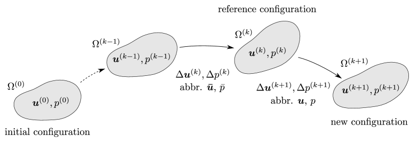
Figure 1: Updated Lagrangian Formulation: scheme of updating domain $\Omega$, notation of displacement and pressure fields and increments at a given time level.

4 Homogenization

Using the two-scale homogenization based on the asymptotic analysis of the deformation-diffusion problem stated above for $\varepsilon\rightarrow 0$, we derive a limit model describing the medium macroscopic response. by virtue of the homogenization, the spatial coordinates can be split into the macroscopic parts denoted by $x$ and the local (microscopic) parts, denoted by $y$. As the consequence of the finite deformation and the incremental formulation, an updated configuration is established in terms of the locally representative periodic deformed cell.

4.1 Locally periodic microstructures and incremental formulations

Since the reference configuration is associated with the deformed structure, this latter is not periodic in general as the result of the nonuniform deformation. In order to apply the tools of the “periodic” homogenization, the notion of locally periodic structures must be introduced. In fact, the results of the asymptotic analysis due to the two-scale convergence or periodic unfolding methods [15] can be obtained even for microsctructures which vary with the macroscopic position $x\in\Omega$ in the deformed configuration. In particular, the so-called slowly varying quasi-periodic structures [10, 9] present a convenient approximate representation of real media. For large deforming media, the computational algorithm associated with a time discretization $\{t_{k}\}_{k}$ is based on an incremental formulation which enables to determine configurations at time $t_{k}+\delta t$ based on information available in past, i.e. for $t\leq t_{k}$.

In this paper we consider an incremental two-scale formulation established using the homogenization of the incremental problem for the “locally periodic” heterogeneous medium. In contrast with linear problems, see e.g. [40, 9], the local periodicity property must be updated during time-stepping, or iterations of solving the nonlinear problem. For a given scale $\varepsilon$, by $Y^{\varepsilon}=\varepsilon Y$ refer to the RVE which coincides with the representative periodic cell $Y$ defined usually as a parallelepiped; for simplicity, we consider $Y=]-\frac{1}{2},\frac{1}{2}[^{3}$ (for the 3D structures) The periodic heterogeneous material is represented by the microconfiguration $\mathcal{M}^{\varepsilon}(x,Y,{\mathbb{H}},\SS)$ describing the continuum occupying domain $Y^{\varepsilon}(x)$ located at position $x$, whereby its material (mechanical) properties are given by ${\mathbb{H}}^{\varepsilon}$ comprising all material parameters, whereas $\SS^{\varepsilon}$ determines the state variables; both ${\mathbb{H}}^{\varepsilon}$ and $\SS^{\varepsilon}$ are functions defined in $Y^{\varepsilon}$. Note that both ${\mathbb{H}}^{\varepsilon}$ and $\SS^{\varepsilon}$ depend on the scale, in general, however, below we drop the superscript ^ε to lighten the notation.

Local periodicity and the computational procedure

The assumption of the local periodicity relying on the slowly varying microconfigurations is needed to homogenize the incremental problem defined by the linearization and time discretization of the evolutionary problem. According to the spatial discretization based on the finite element method, the microconfigurations $\hat{\mathcal{M}}(\hat{x},\hat{Y},\hat{\mathbb{H}},\hat{\SS})$ are established at any selected node $\hat{x}$ associated with the spatial discretization of the macroscopic problem, such as the integration points $\hat{x}$, or finite elements $E(\hat{x})$ “centered” at $\hat{x}$. Intuitively, the local periodicity can be considered within $E(\hat{x})$, or in a neighbourhood $\mathcal{U}_{\delta}^{\varepsilon}(\tilde{x})$ of the (macroscopic) integration point.

The incremental two-scale formulation for the homogenized medium is related to the original hetrogeneous one by virtue of some notions explained in the text below, which are involved in the following time-stepping algorithm:

Algorithm 1 Time-stepping algorithm

1. Time level $t_{k}$: Given a consistent heterogeneous medium for a given scale $\varepsilon=\varepsilon_{0}>0$, establish an approximate locally periodic structure $\mathcal{L}^{\varepsilon}$, see (25), in a $\delta$-neighbourhood $\mathcal{U}_{\delta}^{\varepsilon}(\tilde{x})$ of any selected node $\tilde{x}$ associated with the spatial discretization of the macroscopic problem.

2. Using the asymptotic analysis of the incremental problem and the local unfolding within the neighbourhood $\mathcal{U}_{\delta}^{\varepsilon}(\tilde{x})$, establish the homogenized two-scale models for all considered $\tilde{x}$.

3. For all limit microconfigurations $\mathcal{M}^{0}(\tilde{x},\hat{Y},\hat{\mathbb{H}},\hat{\SS})$, solve local problems for the characteristic responses and compute the homogenized coefficients of the macroscopic model.

4. Collecting the information provided by the microconfigurations $\mathcal{M}^{0}(\tilde{x},\hat{Y},\hat{\mathbb{H}},\hat{\SS})$, at all $\tilde{x}$ considered, constitute the macroscopic numerical model of the discretized macroscopic problem which is then solved for the macroscopic increments of the state variables, providing updates $\Delta\SS$ for each microconfiguration $\mathcal{M}^{0}$ at time $t_{k+1}=t_{k}+\delta t$. Update the local RVEs at $\tilde{x}$ and time $t_{k+1}$.

5. Given RVEs at $\tilde{x}$ (the selected nodes associated with the spatial discretization of the macroscopic problem), for the given finite scale $\varepsilon_{0}$, construct an approximate heterogeneous consistent structure using the concept of slowly varying microconfiguration.

6. Updated macroscopic loads, for computing the new time increment, with $k:=k+1$ proceed by step (i).

Although the computational procedure can avoid the reconstruction step (v), an interpolation procedure should be applied after each time increment computations (while solving the local problems for all local microconfigurations and the macroscopic problem) to respect a final scale $\varepsilon_{0}>0$ of the heterogeneous structure. Indeed, this enables to keep the subsequent homogenization at time levels $t_{1},t_{2},\dots$ independent of the spatial discretization and, thus, to avoid artifacts generated by the discretized formulation.

Lattice generating a periodic microstructure of the initial configuration

Let $\Xi^{\varepsilon}$ be a set of points in ${\mathbb{R}}^{3}$ and $\vec{a}^{j}$, $j=1,2,3$ in ${\mathbb{R}}^{3}$ be three non-planar vectors $\vec{a}^{1}\cdot(\vec{a}^{2}\times\vec{a}^{3})\not=0$, such that for any two $\xi,\xi^{\prime}$, there is a $\boldsymbol{k}\in{\mathbb{Z}}^{3}$ which yields the path between the two points $\xi^{\prime}=\xi+\varepsilon k_{j}\vec{a}^{j}$. The periodic (Bravais) lattice $\mathcal{L}_{0}^{\varepsilon}(\Xi^{\varepsilon},Y^{\varepsilon})$ is generated by $\Xi^{\varepsilon}$ and $\varepsilon Y\equiv Y^{\varepsilon}$, where $Y^{\varepsilon}$ is the representative periodic cell (RPC) defined by the parallelepiped $Y$ with its three edges constituted by vectors $\vec{a}^{k}$. By $\mathcal{I}^{\varepsilon}$ we denote the index set of lattice centers (nodes), i.e. $\xi^{j}\in\Xi^{\varepsilon}\Leftrightarrow j\in\mathcal{I}^{\varepsilon}$. We assume that $\Omega_{0}$ is generated by the periodic lattice $\mathcal{L}^{\varepsilon}(\xi^{0},\Xi^{\varepsilon},Y^{\varepsilon})=\mathcal{L}_{0}^{\varepsilon}(\Xi^{\varepsilon},Y^{\varepsilon})$ defined at node $\xi^{0}\in\Xi^{\varepsilon}$, such that

$$\begin{split}\Omega_{0}=\bigcup_{\xi\in\Xi^{\varepsilon}}Y^{\varepsilon}(\xi)\cup\Gamma^{\varepsilon}\;,\quad Y^{\varepsilon}(\xi)\cap Y^{\varepsilon}(\xi^{\prime})=\emptyset\mbox{ for }\xi\not=\xi^{\prime}\in\Xi^{\varepsilon}\;,\\ Y^{\varepsilon}(\xi^{j})=\xi^{0}+\varepsilon(Y+\sum_{l}^{3}k_{l}^{j}\vec{a}^{l})\;,\quad k_{l}^{j}\in{\mathbb{Z}},\;j\in\mathcal{I}^{\varepsilon}\;,\end{split}$$ (23)

where $Y^{\varepsilon}(\xi^{j})$ is defined using $\boldsymbol{k}^{j}$ as the copy of the scaled RPC $\varepsilon Y$ situated at position $\xi$. Above $\Gamma^{\varepsilon}$ is the union of all interfaces $\Gamma_{ij}=\partial Y^{\varepsilon}(\xi^{i})\cap\partial Y^{\varepsilon}(\xi^{j})$, $i,j\in\mathcal{I}^{\varepsilon}$.

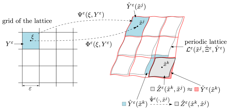
Figure 2: A scheme explaining the meaning of mappings $\Phi^{\varepsilon}$ and $\Psi^{\varepsilon}$ employed to introduce the locally periodic microstructures at the local position $\tilde{x}^{j}$ using the lattice $\mathcal{L}^{\varepsilon}(\hat{x}^{j},\hat{\Xi}^{\varepsilon},\hat{Y}^{\varepsilon})$.

Slowly varying microstructure and deformed configuration

The notion of the slowly varying microstructure has been reported e.g. in [10] in the context of a stationary Stokes flow homogenization, where the microstructure is represented by the geometry only. When dealing with an evolutionary problem of large deforming media, the “slow variation” is influenced by the assumed inhomogeneity of the macroscopic deformation and of other related state variables which determine the actual micro-configurations.

We shall assume that the deformed configuration represents a medium with a slowly varying microstructure, being constituted as the union of cells $\tilde{Y}^{\varepsilon}(x^{j})\equiv\tilde{Y}^{\varepsilon,j}$, such that

$$\begin{split}\Omega&=\bigcup_{j}\tilde{Y}^{\varepsilon}(x^{j})\cup\tilde{\Gamma}^{\varepsilon}\;,\\ \tilde{Y}^{\varepsilon}(\tilde{x})&=\Phi^{\varepsilon}(\xi,Y^{\varepsilon})\;,\quad\tilde{x}=\varphi^{\varepsilon}(\xi)\;,\quad\forall\xi\in\Xi^{\varepsilon}\;,\end{split}$$ (24)

where $\Phi^{\varepsilon}$ is established using a differentiable mapping, $\varphi^{\varepsilon}:\Omega_{0}\mapsto\Omega$. As will be explained below, mapping $\Phi^{\varepsilon}$ is constructed using the unfolding and a folding procedures associated with the homogenization $\varepsilon\rightarrow 0$ and the reconstruction of the homogenized incremental solutions.

Local periodicity and local lattice

The local periodicity property of the microsctructures is needed to apply the homogenization procedure; in [28], a rigorous treatment was explained in terms of the unfolding approach. We can introduce locally periodic microstructures as an approximation of slowly varying microstructures which are assumed to describe the heterogeneous porous medium characterized by a given finite scale $\varepsilon>0$, see Fig. 2. In the limit $\varepsilon\rightarrow 0$, due to the perfect scale separation, the downscaling procedure applied to the homogenized medium yields locally periodic microstructures. These also naturally represent the numerical approximation of the homogenized medium, as explained below.

We shall assume that for any $\tilde{x}=\varphi(\xi)$, such that $\xi\in\Xi^{\varepsilon}$, there exist a neighbourhood $\mathcal{U}_{\delta}^{\varepsilon}(\tilde{x})\subset\Omega$ in which the spatial (deformed) heterogeneous structure can be well approximated by a locally periodic one. For any $\tilde{x}^{j}=\varphi^{\varepsilon}(\xi^{j})$, $\xi^{j}\in\Xi^{\varepsilon}$, there exists the local RPC $\hat{Y}$ defining the lattice $\mathcal{L}^{\varepsilon}(\tilde{x}^{j},\hat{\Xi},\hat{Y})$, such that

$$\begin{split}\hat{Y}^{\varepsilon}(\hat{x}^{k})&=\varepsilon(\hat{Y}+\hat{z}^{k,j})\;,\quad\mbox{ where }\hat{z}^{k,j}=\varepsilon^{-1}(\hat{x}^{k}-\hat{x}^{j})\;,\;\hat{x}^{j}\equiv\tilde{x}^{j}\;,\\ \tilde{Z}^{\varepsilon}(\tilde{x}^{k};\tilde{x}^{j})&=\{x\in\Omega|\;x=\hat{\psi}^{\varepsilon}(\hat{x},\tilde{x}^{j}),\;\mbox{ for }\hat{x}\in\hat{Y}^{\varepsilon}(\hat{x}^{k})\}\;,\\ \end{split}$$ (25)

such that $\hat{\psi}^{\varepsilon}(\cdot,\tilde{x}^{j})$ is a diffeomorphism mapping the positions in the local periodic structure on the spatial positions. Hence, $\tilde{Z}^{\varepsilon}(\tilde{x}^{k};\tilde{x}^{j})\approx\tilde{Y}^{\varepsilon}(\tilde{x}^{k})=\Phi^{\varepsilon}(\xi^{k},Y^{\varepsilon})$. Below we introduce RPC $\hat{Y}^{\varepsilon}(\hat{x}^{j})$ as an (in a sense, the best) approximation of $\tilde{Y}^{\varepsilon}(\tilde{x}^{j})$, see problem (29). Consequently, the local lattice $\mathcal{L}^{\varepsilon}(\hat{x}^{j},\hat{\Xi}^{\varepsilon},\hat{Y}^{\varepsilon})$ can be defined. Domain $\hat{Y}^{\varepsilon}$ can be considered as the image of a $Y$-periodic regular mapping of cell $\varepsilon Y$.

It should be noted that cells $\tilde{Z}^{\varepsilon}(\tilde{x}^{k},\tilde{x}^{j})$ at a fixed position $\tilde{x}^{k}$ can be introduced using different locally periodic approximations when choosing different $\tilde{x}^{j}$. This constitutes the basis for the homogenization.

Besides the geometry (i.e. the RVE decomposition into various compartments occupied by different phases), the deformed structure is characterized by its parameters and state variables (fields). Therefore, the approximation property must respect the “microconfiguration”, as introduced above. Let $\tilde{\mathcal{M}}^{\varepsilon}(\tilde{x},\tilde{Y}^{\varepsilon},\tilde{\mathbb{H}},\tilde{\SS})$ be the spatial configuration associated with domain $\tilde{Y}^{\varepsilon}(\tilde{x})$. For $\varepsilon>0$, we can establish an approximation $\hat{\mathcal{M}}^{\varepsilon}(\tilde{x},\hat{Y},\hat{\mathbb{H}},\hat{\SS})\approx\tilde{\mathcal{M}}^{\varepsilon}(\tilde{x},\tilde{Y}^{\varepsilon},\tilde{\mathbb{H}},\tilde{\SS})$. By $\hat{g}$ we denote a function defined in the local lattice $\mathcal{L}^{\varepsilon}(\hat{x},\hat{\Xi},\hat{Y})$ with $\hat{x}=\tilde{x}$ and $\tilde{g}^{\varepsilon}$ the corresponding function defined in the spatial configuration $\Omega$. In general, $\hat{g}$ can be decomposed into a periodic part, $\hat{g}_{\#}(y,\hat{x})$, $y\in\hat{Y}$, and a macroscopic part, $\hat{g}_{G}(x,\tilde{x})$, $x\in Y^{\varepsilon}(\tilde{x})$, thus,

$$\begin{split}{\mathcal{T}}_{\varepsilon}{\left({\hat{g}^{\varepsilon}(x)}\right)}&:=\hat{g}_{\#}(y,\tilde{x})\hat{g}_{G}(x,\tilde{x})\;,\quad\tilde{x}=\hat{x}\;,\end{split}$$ (26)

where ${\mathcal{T}}_{\varepsilon}{\left({}\right)}$ is the unfolding operator [15], cf. [28]. We assume the following approximation property is satisfied by $\tilde{g}^{\varepsilon}$,

$$\begin{split}\|{\mathcal{T}}_{\varepsilon}{\left({\tilde{g}^{\varepsilon}(\hat{\psi}^{\varepsilon}(\varepsilon\cdot,\tilde{x}^{j}))}\right)}-{\mathcal{T}}_{\varepsilon}{\left({\hat{g}^{\varepsilon}}\right)}\|_{L^{2}(\hat{Y})}&\rightarrow 0\quad\mbox{ for }\varepsilon\rightarrow 0\;,\end{split}$$ (27)

where $\varepsilon\cdot$ is substituted by $\varepsilon y$, $y\in\hat{Y}$.

In the generic sense, function $\tilde{g}^{\varepsilon}$ represents any material, or state function of $\tilde{\mathcal{M}}^{\varepsilon}(\tilde{x},\tilde{Y}^{\varepsilon},\cdot,\cdot)$, whereas $\hat{g}^{\varepsilon}$ is the corresponding approximation.

Reconstruction of continuously varying microstructure for $\varepsilon_{0}>0$

It is well known, that, in the numerical homogenization, the microstructures are associated with the discretization scheme. As will be shown below, an incremental algorithm can be designed which uses the limit two-scale model and the computation is based on alternating micro- and macro steps. In the context of such an incremental formulation providing responses at time $t+\delta t$ based on a known configuration at time $t$, it is desirable to establish a link between the deformed heterogeneous medium and the homogenized medium for which the assumption of a locally periodic microstructure is needed. For this there are two reasons at least: 1) the homogenization of a heterogeneous medium at time $t$ independently of the numerical approximation, 2) reconstructions of the homogenized responses for a given scale.

Therefore, we suggest a “downscaling” procedure, see step (v) of the Algorithm A1, which enables to reconstruct the heterogeneous structures based on locally periodic microconfigurations established by virtue of the homogenization, step (ii) of the Algorithm A1. For this, we first need to introduce the representative periodic cell of the locally periodic microstructure which represents the actual “slowly varying” microstructure $\tilde{Y}^{\varepsilon}(\tilde{x}^{k})$. There exist mappings $\tilde{\varphi}^{\varepsilon}$ and $\Psi^{\varepsilon}$, such that

$$\begin{split}\tilde{\varphi}^{\varepsilon}:\tilde{Y}^{\varepsilon}(\tilde{x}^{k})&\mapsto\hat{Y}^{\varepsilon}(\hat{x}^{k})\;,\\ \hat{Y}^{\varepsilon}(\hat{x}^{k})&=\Psi^{\varepsilon}(\xi,Y^{\varepsilon})\;,\quad\hat{x}^{k}=\varphi^{\varepsilon}(\xi)\;,\quad\xi\in\Xi^{\varepsilon}\;,\end{split}$$ (28)

thus, $\hat{Y}^{\varepsilon}$ is the deformed cell $Y^{\varepsilon}$ at the lattice point $\xi$ of the inital configuration. Mapping $\tilde{\varphi}^{\varepsilon}$ is introduced by virtue of the following minimization problem: Find $\Psi^{\varepsilon}(\xi,\cdot)\in{\bf{H}}_{\#}^{1}(Y^{\varepsilon})$ such that

$$\begin{split}\|\Phi^{\varepsilon}(\xi,\cdot)-\Psi^{\varepsilon}(\xi,\cdot)\|_{{\bf{L}}^{2}(Y^{\varepsilon})}\rightarrow\min.\end{split}$$ (29)

Alternatively, the ${\bf{L}}^{2}(\mathcal{U}_{\delta}^{\varepsilon}(\tilde{x}))$ norm can be employed together with the lattice $\mathcal{L}^{\varepsilon}(\tilde{x},\hat{\Xi}^{\varepsilon},\hat{Y}^{\varepsilon})$ established by virtue of (25),

$$\begin{split}\|{\mathcal{T}}_{\varepsilon}{\left({\Phi^{\varepsilon}(\xi,\cdot)}\right)}-\Psi(\xi,\cdot,\cdot)\|_{\mathcal{U}_{\delta}^{\varepsilon}(\tilde{x})\times\hat{Y}}\rightarrow\min,\end{split}$$ (30)

where scale is fixed $\varepsilon:=\varepsilon_{0}>0$ and $\Psi(\xi,x,y)={\mathcal{T}}_{\varepsilon}{\left({\Psi^{\varepsilon}(\xi,x)}\right)}$ is the two-scale $\hat{Y}$-periodic function.

For a given $\varepsilon_{0}$, the characteristic microstructure size $\ell^{\varepsilon_{0}}<<h$, where $h>0$ is the perimeter of the finite element, a locally periodic microstructures, or the slowly varying microstructures can be established using problem (29).

• A) The locally periodic microstructure defined within a subdomain $\Omega_{h}(\tilde{x}^{j})\subset\mathcal{U}_{\delta}^{\varepsilon_{0}}(\tilde{x}^{j})$ which can be associated with a finite element $E_{h}(\tilde{x}^{j})$ “located” at $\tilde{x}^{j}$ whose the perimeter is $h$.

• B) The slowly varying microstructure introduced via an approximation $\tilde{\Psi}^{\varepsilon_{0}}(\{\tilde{x}^{k}\}_{k\in\mathcal{I}_{h}^{\varepsilon_{0}}},\cdot)$ which is constructed as an interpolation of the locally periodic microstructures defined at selected points $\{\tilde{x}^{k}\}_{k\in\mathcal{I}_{h}^{\varepsilon_{0}}}$.

Recall that in both the cases, the geometrical transformations related to cells $\hat{Y}^{\varepsilon}$ are employed as the basis for the approximation of microconfigurations $\tilde{\mathcal{M}}^{\varepsilon}(\tilde{x},\tilde{Y}^{\varepsilon},\cdot,\cdot)$.

4.2 Reference cell decomposition and double porosity

By $Y$ we now abbreviate the local spatial reference cell $\varepsilon^{-1}Y^{\varepsilon}$, without writing explicitly the macroscopic location. Since our interests are in porous media with large contrasts in the permeability coefficients, we shall introduce the following decomposition of $Y$ into the sectors of primary and dual porosities.

Let $Y_{\alpha}$, for $\alpha=1,2$ be mutually disconnected subdomains of $Y$ with Lipschitz boundary, then $Y_{3}$ forms the complement (see Fig. 3)

$$Y_{3} \equiv Y\setminus\bigcup_{\alpha=1,2}\overline{Y_{\alpha}},$$ (31)

$$\Gamma_{\alpha}=\partial_{3}Y_{\alpha}=\partial_{\alpha}Y_{3} \equiv\overline{Y_{\alpha}}\cap\overline{Y_{3}}.$$

Furthermore, we require that $\partial Y\cap\partial Y_{l}\not=\emptyset$, so that the all domains $\Omega_{l}^{\varepsilon}$, $l=1,2,3$ generated by repeating the cells $\varepsilon Y_{l}$ are connected. The parts of the periodic boundary will be denoted by

$$\partial_{l}Y=\partial_{l}Y_{l}\equiv\overline{Y_{l}}\cap\partial Y\;,\quad l=1,2,3\;.$$ (32)

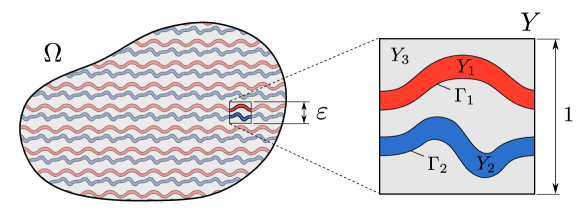
Figure 3: The macroscopic domain $\Omega$ and the representative cell $Y$ constituted by the porous matrix $Y_{3}$ and two fluid channels $Y_{1}$, $Y_{2}$.

The material parameters in deformed configuration depend on the deformation. To define them in the local reference cell, we use the unfolding operation, [14]. For the sake of brevity, we shall consider couples $(y,x)$ implicitly matching, such that $y-\hat{y}=\varepsilon^{-1}(x-\hat{x})$. In the spatial configuration we introduce the permeability parameters, as follows:

$$\boldsymbol{K}^{\varepsilon}(x)=\left\{\begin{array}[]{ll}\tilde{\boldsymbol{K}}^{\alpha}(x,y)&y\in Y_{\alpha},\;\alpha=1,2,\\ \varepsilon^{2}\tilde{\boldsymbol{K}}^{3}(x,y)&y\in Y_{3}\;.\end{array}\right.$$ (33)

Symbol $\tilde{}$ denotes quantities that are expressed using the unfolded spatial coordinates $x$, $y$. We emphasize, that the scaling of the permeability coefficients by $\varepsilon^{2}$ in the “matrix” compartment leads to the double porosity effect.

Remark.

Obviously, in the large deformation regime, tensors $\tilde{\boldsymbol{K}}^{l}$ should be given as functions of the material deformation and, thus, should be modified in time, as the deformation progresses. By virtue of the homogenization, the local microscopic deformation gradients are introduced, so that the permeabilities can be updated at each time level.

4.3 Asymptotic expansions and two scale decompositions

The linearized problem can be treated using the standard homogenization techniques, such as the periodic unfolding, the two scale convergence, or even the asymptotic expansion methods.

The displacement and pressure increments $\boldsymbol{u}^{\varepsilon}$ and $p^{\varepsilon}$ can be expressed by the following truncated expansions:

$$\boldsymbol{u}^{\varepsilon}(x) =\boldsymbol{u}^{0}(x)+\varepsilon\boldsymbol{u}^{1}(x,y)+O(\varepsilon^{2}),$$ (34)

$$p^{\varepsilon}(x) =\sum_{\alpha=1,2}\chi_{\alpha}(y)\left(p_{\alpha}^{0}(x)+\varepsilon p_{\alpha}^{1}(x,y)+O(\varepsilon^{2})\right)+\chi_{3}(y)\left(p_{3}(x,y)+O(\varepsilon)\right),$$

where we respect the abbreviated notation (18) and $\chi_{l}$ is the characteristic function of subdomain $Y_{l}$ such that $\chi_{l}(y)=1$ in $Y_{l}$ whereas $\chi_{l}(y)=0$ in $Y\setminus Y_{l}$.

Upon substituting these expansions into (21)–(22) and using the unfolding technique or the two-scale convergence method, we obtain the limit problem (for $\varepsilon\rightarrow 0$) formed by the coupled system involving the unknown displacement increments $(\boldsymbol{u}^{0},\boldsymbol{u}^{1})\in\boldsymbol{V}\kern-2.5pt_{0}(\Omega)\times L^{2}(\Omega;{\bf H}_{\#}^{1}(Y))$ and the pressure increments $(p^{0}_{\alpha},p^{1}_{\alpha})\in H^{1}(\Omega)\times L^{2}(\Omega;H_{\#}^{1}(Y_{\alpha})))$, $\alpha=1,2$, $p_{3}\in L^{2}(\Omega;H_{\#0}^{1}(Y_{3}))$:

$$\int_{\Omega}\fint_{Y} \left[\boldsymbol{\mathbb{A}}\left(\nabla_{x}\boldsymbol{u}^{0}+\nabla_{y}\boldsymbol{u}^{1}\right)-(\sum_{\alpha=1,2}\chi_{\alpha}p_{\alpha}^{0}+\chi_{3}p_{3})(\tilde{\boldsymbol{B}}(\bar{\boldsymbol{u}})+\boldsymbol{I})\right]:\left(\nabla_{x}\boldsymbol{v}^{0}+\nabla_{y}\boldsymbol{v}^{1}\right)$$ (35)

$$= \int_{\Omega}\fint_{Y}\hat{\boldsymbol{\sigma}}:\left(\nabla_{x}\boldsymbol{v}^{0}+\nabla_{y}\boldsymbol{v}^{1}\right)+\int_{\Omega}\fint_{Y}\boldsymbol{f}^{new}\cdot\boldsymbol{v}^{0},$$

$$\int_{\Omega}\fint_{Y} (\sum_{\alpha=1,2}\chi_{\alpha}q_{\alpha}^{0}+\chi_{3}q_{3})(\tilde{\boldsymbol{B}}(\bar{\boldsymbol{u}})+\boldsymbol{I}):\left(\nabla_{x}\boldsymbol{u}^{0}+\nabla_{y}\boldsymbol{u}^{1}\right)$$ (36)

$$+\delta t\int_{\Omega}\fint_{Y_{3}}\left[\tilde{\boldsymbol{K}}^{3}+\tilde{\boldsymbol{H}}^{3}(\bar{\boldsymbol{u}})\right]\nabla_{y}p_{3}\cdot\nabla_{y}q_{3}$$

$$+\delta t\int_{\Omega}\sum_{\alpha=1,2}\fint_{\alpha}\left[\tilde{\boldsymbol{K}}^{\alpha}+\tilde{\boldsymbol{H}}^{\alpha}(\bar{\boldsymbol{u}})\right](\nabla_{x}p_{\alpha}^{0}+\nabla_{y}p_{\alpha}^{1})\cdot(\nabla_{x}q_{\alpha}^{0}+\nabla_{y}q_{\alpha}^{1})$$

$$= -\delta t\int_{\Omega}\fint_{Y_{3}}\left[\tilde{\boldsymbol{K}}^{3}+\tilde{\boldsymbol{H}}^{3}(\bar{\boldsymbol{u}})+\delta\tilde{\boldsymbol{K}}^{3}\right]\nabla_{y}\hat{p}_{3}\cdot\nabla_{y}q_{3}$$

$$-\delta t\int_{\Omega}\sum_{\alpha=1,2}\fint_{\alpha}\left[\tilde{\boldsymbol{K}}^{\alpha}+\tilde{\boldsymbol{H}}^{\alpha}(\bar{\boldsymbol{u}})+\delta\tilde{\boldsymbol{K}}^{\alpha}\right](\nabla_{x}\hat{p}_{\alpha}^{0}+\nabla_{y}\hat{p}_{\alpha}^{1})\cdot(\nabla_{x}q_{\alpha}^{0}+\nabla_{y}q_{\alpha}^{1}),$$

where $\nabla_{x}$ and $\nabla_{y}$ are the partial gradients with respect to the macroscopic and microscopic coordinates. The quantities at the right hand sides used at time $t$, i.e. $\boldsymbol{\sigma}^{(k)}$, $p_{3}^{(k)}$, $(p_{\alpha}^{0})^{(k)}$, $(p_{\alpha}^{1})^{(k)}$, are labelled by symbol $\hat{\ }$ to avoid the double upper indices in the notation. The average integral for any $Y_{l}\subset Y$, for the subdomain index $l=1,2,3$, is abbreviated by

$$\fint_{Y_{l}}f=\frac{1}{|Y|}\int_{Y_{l}}f.$$ (37)

Tensors $\tilde{\boldsymbol{B}}$, $\tilde{\boldsymbol{H}}^{l}$ depending on a two-scale vector fields $\boldsymbol{v}=(\boldsymbol{v}^{0},\boldsymbol{v}^{1})$ are defined as follows:

$$\tilde{\boldsymbol{B}}(\boldsymbol{v}) =(\boldsymbol{I}\otimes\boldsymbol{I}-\boldsymbol{\mathbb{I}})\left(\nabla_{x}\boldsymbol{v}^{0}+\nabla_{y}\boldsymbol{v}^{1}\right),$$ (38)

$$\tilde{\boldsymbol{H}}^{l}(\boldsymbol{v}) =(\nabla_{x}\cdot\boldsymbol{v}^{0}+\nabla_{y}\cdot\boldsymbol{v}^{1})\tilde{\boldsymbol{K}}^{l}-\tilde{\boldsymbol{K}}^{l}(\nabla_{x}\boldsymbol{v}^{0}+\nabla_{y}\boldsymbol{v}^{1})^{T}-(\nabla_{x}\boldsymbol{v}^{0}+\nabla_{y}\boldsymbol{v}^{1})(\tilde{\boldsymbol{K}}^{l})^{T}.$$

By $H^{1}(\Omega)$ we denote the standard Sobolev space $W^{1,2}(\Omega)$, $H_{\#}^{1}(Y)$ is the functional space of $Y$-periodic functions, ${\bf H}_{\#}^{1}(Y)$ is the generalization for vector functions and $H_{\#0}^{1}(Y_{3})$ includes all functions from $H_{\#}^{1}(Y_{3})$ that are zero on the boundary $\Gamma_{3}$.

Due to the linearity of the limit equations, we can define the decomposition of the fluctuating functions, introducing the characteristic responses $\boldsymbol{\omega}$, $\pi$, $\eta$ and the particular responses $\boldsymbol{u}^{P}$, $p_{l}^{P}$ depending on the actual pressures and stresses,

$$\boldsymbol{u}^{1} =\boldsymbol{\omega}^{ij}\partial_{j}^{x}u_{i}^{0}+\sum_{\alpha=1,2}\boldsymbol{\omega}^{\alpha}p_{\alpha}^{0}+\boldsymbol{u}^{P},$$ (39)

$$p_{3} =\pi^{ij}\partial_{j}^{x}u_{i}^{0}+\sum_{\alpha=1,2}\pi^{\alpha}p_{\alpha}^{0}+p_{3}^{P},$$

$$p_{\alpha}^{1} =\eta_{\alpha}^{i}\partial_{i}^{x}p_{\alpha}^{0}+p_{\alpha}^{P}.$$

4.4 Local microscopic subproblems

Further, to simplify the notation, we shall employ the following linear and bilinear forms:

$$a_{Y}\left(\boldsymbol{u},\boldsymbol{v}\right) =\fint_{Y}\boldsymbol{\mathbb{A}}\nabla_{y}\boldsymbol{u}:\nabla_{y}\boldsymbol{v}=\fint_{Y}\boldsymbol{\mathbb{A}}\boldsymbol{e}_{y}({\boldsymbol{u}}):\boldsymbol{e}_{y}({\boldsymbol{v}}),$$ (40)

$$b_{Y_{l}}\left(\bar{\boldsymbol{u}};q,\boldsymbol{u}\right) =\fint_{Y_{l}}q\left[\tilde{\boldsymbol{B}}(\bar{\boldsymbol{u}})+\boldsymbol{I}\right]:\nabla_{y}\boldsymbol{u},$$

$$c_{Y_{l}}\left(\bar{\boldsymbol{u}};p,q\right) =\fint_{Y_{l}}\left[\tilde{\boldsymbol{K}}^{l}+\tilde{\boldsymbol{H}}^{l}(\bar{\boldsymbol{u}})\right]:\nabla_{y}p\cdot\nabla_{y}q,$$

$$d_{Y_{l}}\left(p,q\right) =\fint_{Y_{l}}\delta\tilde{\boldsymbol{K}}^{l}\nabla_{y}p\cdot\nabla_{y}q,$$

$$g_{3}^{\alpha}(\bar{\boldsymbol{u}};p) =\int_{\Gamma_{\alpha}}\left(\tilde{\boldsymbol{K}}^{3}+\tilde{\boldsymbol{H}}(\bar{\boldsymbol{u}})\right)\nabla_{y}p\cdot\boldsymbol{n}^{3}\mathrm{\,dS}_{y},$$

defined for $l=1,2,3$ and for $\alpha=1,2$. By $\boldsymbol{n}^{3}$ we denote the normal unit vector on boundary $\Gamma_{\alpha}=\overline{Y_{\alpha}}\cap\overline{Y_{3}}$ oriented outwards of $Y_{3}$. Note that all integrals are defined in the reference deformed configuration.

The microscopic equations are obtained from (35)–(36) by letting vanish all the macroscopic test functions,

$$a_{Y}\left(\boldsymbol{\Pi}:\nabla_{x}\boldsymbol{u}^{0}+\boldsymbol{u}^{1},\boldsymbol{v}\right)-\sum_{\alpha=1,2}b_{Y_{\alpha}}\left(\bar{\boldsymbol{u}};p^{0}_{\alpha},\boldsymbol{v}\right)-b_{Y_{3}}\left(\bar{\boldsymbol{u}};p_{3},\boldsymbol{v}\right)=-\fint_{Y}\hat{\boldsymbol{\sigma}}:\nabla_{y}\boldsymbol{v},$$ (41)

$$b_{Y_{3}}\left(\bar{\boldsymbol{u}};q,\boldsymbol{\Pi}:\nabla_{x}\boldsymbol{u}^{0}+\boldsymbol{u}^{1}\right)+\delta tc_{Y_{3}}\left(\bar{\boldsymbol{u}};p_{3},q\right)=-\delta t\left[c_{Y_{3}}\left(\bar{\boldsymbol{u}};\hat{p}_{3},q\right)+d_{Y_{3}}\left(\hat{p}_{3},q\right)\right],$$

holding for all $\boldsymbol{v}\in{\bf H}_{\#}^{1}(Y)$ and $q\in H_{\#}^{1}(Y_{3})$, and

$$c_{Y_{\alpha}}\left(\bar{\boldsymbol{u}};\boldsymbol{y}\cdot\nabla_{x}p_{\alpha}^{0}+p_{\alpha}^{1},q\right)=-c_{Y_{\alpha}}\left(\bar{\boldsymbol{u}};\boldsymbol{y}\cdot\nabla_{x}\hat{p}_{\alpha}^{0}+\hat{p}_{\alpha}^{1},q\right)-d_{Y_{\alpha}}\left(\boldsymbol{y}\cdot\nabla_{x}\hat{p}_{\alpha}^{0}+\hat{p}_{\alpha}^{1},q\right),$$ (42)

for all $q\in H_{\#}^{1}(Y_{\alpha})$. Above, we use tensor $\boldsymbol{\Pi}=(\Pi^{rs}_{i})$ with components $\Pi^{rs}_{i}=y_{s}\delta_{ir}$ that involve the microscopic coordinates $\boldsymbol{y}$.

Employing the two-scale decompositions (39) in equations (41)–(42) enables us to extract the local problems for the characteristic responses $\boldsymbol{\omega},\pi$ and $\eta$. The following problems associated with the poroelasticity in the whole cell $Y$ and perfusion in the dual porosity $Y_{3}$ must be resolved for a given time step increment $\delta t$:

1. Find $(\boldsymbol{\omega}^{ij},\pi^{ij})\in{\bf H}_{\#}^{1}(Y)\times H_{\#0}^{1}(Y_{3})$ such that

   $$a_{Y}\left(\boldsymbol{\omega}^{ij}+\boldsymbol{\Pi}^{ij},\boldsymbol{v}\right)-b_{Y_{3}}\left(\bar{\boldsymbol{u}};\pi^{ij},\boldsymbol{v}\right) =0,\quad \forall\boldsymbol{v}\in{\bf H}_{\#}^{1}(Y),$$ (43)

   $$b_{Y_{3}}\left(\bar{\boldsymbol{u}};q,\boldsymbol{\omega}^{ij}+\boldsymbol{\Pi}^{ij}\right)+\delta tc_{Y_{3}}\left(\bar{\boldsymbol{u}};\pi^{ij},q\right) =0, \forall q\in H_{\#0}^{1}(Y_{3}).$$

2. Find $(\boldsymbol{\omega}^{\alpha},\pi^{\alpha})\in{\bf H}_{\#}^{1}(Y)\times H_{\#}^{1}(Y_{3})$ such that

   $$a_{Y}\left(\boldsymbol{\omega}^{\alpha},\boldsymbol{v}\right)-b_{Y_{3}}\left(\bar{\boldsymbol{u}};\pi^{\alpha},\boldsymbol{v}\right) =b_{Y_{\alpha}}\left(\bar{\boldsymbol{u}};1,\boldsymbol{v}\right),\quad \forall\boldsymbol{v}\in{\bf H}_{\#}^{1}(Y),$$ (44)

   $$b_{Y_{3}}\left(\bar{\boldsymbol{u}};q,\boldsymbol{\omega}^{\alpha}\right)+\delta tc_{Y_{3}}\left(\bar{\boldsymbol{u}};\pi^{\alpha},q\right) =0, \forall q\in H_{\#0}^{1}(Y_{3}),$$

   where (in the sense of traces) $\pi^{\alpha}=\delta_{\alpha\beta}$ on $\Gamma_{\beta}$.

3. Find $(\boldsymbol{u}^{P},p_{3}^{P})\in{\bf H}_{\#}^{1}(Y)\times H_{\#0}^{1}(Y_{3})$, the particular response to the current reference state, such that

   $$a_{Y}\left(\boldsymbol{u}^{P},\boldsymbol{v}\right)-b_{Y_{3}}\left(\bar{\boldsymbol{u}};p_{3}^{P},\boldsymbol{v}\right) =-\fint_{Y}\hat{\boldsymbol{\sigma}}:\nabla_{y}\boldsymbol{v},\quad \forall\boldsymbol{v}\in{\bf H}_{\#}^{1}(Y),$$ (45)

   $$b_{Y_{3}}\left(\bar{\boldsymbol{u}};q,\boldsymbol{u}^{P}\right)+\delta tc_{Y_{3}}\left(\bar{\boldsymbol{u}};p_{3}^{P},q\right) =-\delta t\left(c_{Y_{3}}\left(\bar{\boldsymbol{u}};\hat{p}_{3},q\right)+d_{Y_{3}}\left(\hat{p}_{3},q\right)\right), \forall q\in H_{\#0}^{1}(Y_{3}).$$

The following two microscopic subproblems are related to the fluid channels $Y_{\alpha}$, $\alpha=1,2$:

1. The channel flow correctors: Find $\eta_{\alpha}^{i}\in H_{\#}^{1}(Y_{\alpha})$ such that

   $$c_{Y_{\alpha}}\left(\bar{\boldsymbol{u}};\eta_{\alpha}^{i}+y_{i},q\right)=0,\quad\forall q\in H_{\#}^{1}(Y_{\alpha}).$$ (46)

2. The particular response for the current load response: Find $p_{\alpha}^{P}\in H_{\#}^{1}(Y_{\alpha})$, such that

   $$c_{Y_{\alpha}}\left(\bar{\boldsymbol{u}};p_{\alpha}^{P},q\right)=d_{Y_{\alpha}}\left(\boldsymbol{y}\cdot\nabla_{x}\hat{p}_{\alpha}^{0}+\hat{p}_{\alpha}^{1},q\right)-c_{Y_{\alpha}}\left(\bar{\boldsymbol{u}};\boldsymbol{y}\cdot\nabla_{x}\hat{p}_{\alpha}^{0}+\hat{p}_{\alpha}^{1},q\right),\quad\forall q\in H_{\#}^{1}(Y_{\alpha}).$$ (47)

4.5 Global macroscopic problem and the homogenized coefficients

The global macroscopic equations and the homogenized coefficients are obtained from system (35)–(36) applying the macroscopic test functions $\boldsymbol{v}^{0}$, $q^{0}_{\alpha}$ and taking $\boldsymbol{v}^{1}=0$, $q^{1}_{\alpha}=0$, but $q_{3}=0$ in $Y_{3}$ and $q_{3}=q^{0}_{\alpha}$ on $\Gamma_{\alpha}$. The balance of forces equation attains the following form:

$$\int_{\Omega}\fint_{Y} \left[\boldsymbol{\mathbb{A}}\nabla_{y}(\boldsymbol{\Pi}:\nabla_{x}\boldsymbol{u}^{0}+\boldsymbol{u}^{1})-\left(\sum_{\alpha=1,2}\chi_{\alpha}p_{\alpha}^{0}+\chi_{3}p_{3}\right)(\tilde{\boldsymbol{B}}(\bar{\boldsymbol{u}})+\boldsymbol{I})\right]:\nabla_{y}(\boldsymbol{\Pi}:\nabla_{x}\boldsymbol{v}^{0})$$ (48)

$$= \int_{\Omega}\fint_{Y}\hat{\boldsymbol{\sigma}}:\nabla_{x}\boldsymbol{v}^{0}+\int_{\Omega}\fint_{Y}\boldsymbol{f}^{\rm new}\cdot\boldsymbol{v}^{0}$$

and the diffusion equation results in two limit equations for $\alpha=1,2$

$$\int_{\Omega}\fint_{\alpha} q_{\alpha}^{0}\left[\tilde{\boldsymbol{B}}(\bar{\boldsymbol{u}})+\boldsymbol{I}\right]:\nabla_{y}(\boldsymbol{\Pi}:\nabla_{x}\boldsymbol{u}^{0}+\boldsymbol{u}^{1})+\delta t\int_{\Omega}q^{0}_{\alpha}g_{3}^{\alpha}(\bar{\boldsymbol{u}};p_{3})$$ (49)

$$+\delta t\int_{\Omega}\fint_{\alpha}\left[\tilde{\boldsymbol{K}}^{\alpha}+\tilde{\boldsymbol{H}}^{\alpha}(\bar{\boldsymbol{u}})\right]\nabla_{y}(\boldsymbol{y}\cdot\nabla_{x}p_{\alpha}^{0}+p_{\alpha}^{1})\cdot\nabla_{x}q_{\alpha}^{0}$$

$$= -\delta t\int_{\Omega}q^{0}_{\alpha}\left(g_{3}^{\alpha}(\bar{\boldsymbol{u}};\hat{p}_{3})+\int_{\Gamma_{\alpha}}\delta\tilde{\boldsymbol{K}}^{3}\nabla_{y}\hat{p}_{3}\cdot\boldsymbol{n}^{3}\mathrm{\,dS}_{y}\right)$$

$$-\delta t\int_{\Omega}\fint_{\alpha}\left[\tilde{\boldsymbol{K}}^{\alpha}+\tilde{\boldsymbol{H}}^{\alpha}(\bar{\boldsymbol{u}})+\delta\tilde{\boldsymbol{K}}^{\alpha}\right]\nabla_{y}(\boldsymbol{y}\cdot\nabla_{x}\hat{p}_{\alpha}^{0}+\hat{p}_{\alpha}^{1})\cdot\nabla_{y}(\boldsymbol{y}\cdot\nabla_{x}q_{\alpha}^{0}),$$

where we use the linear form

$$g_{3}^{\alpha}(\bar{\boldsymbol{u}};p)=\int_{\Gamma_{\alpha}}\left(\tilde{\boldsymbol{K}}^{3}+\tilde{\boldsymbol{H}}(\bar{\boldsymbol{u}})\right)\nabla_{y}p\cdot\boldsymbol{n}^{3}\mathrm{\,dS}_{y}.$$ (50)

Upon substituting the microscopic fluctuations $\boldsymbol{u}^{1}$ and $p_{3}$ in the equilibrium equation (48) by the decompositions defined in (39), the following homogenized coefficients can be introduced:

• The effective viscoelastic incremental tensor, $\boldsymbol{\mathcal{D}}=(\mathcal{D}_{ijkl})$,

  $$\mathcal{D}_{ijkl} =|Y|^{-1}\left[a_{Y}\left(\boldsymbol{\omega}^{kl}+\boldsymbol{\Pi}^{kl},\boldsymbol{\Pi}^{ij}\right)-b_{Y_{3}}\left(\bar{\boldsymbol{u}};\pi^{kl},\boldsymbol{\Pi}^{ij}\right)\right]$$ (51)

  $$=|Y|^{-1}\left[a_{Y}\left(\boldsymbol{\omega}^{kl}+\boldsymbol{\Pi}^{kl},\boldsymbol{\omega}^{ij}+\boldsymbol{\Pi}^{ij}\right)+\delta tc_{Y_{3}}\left(\bar{\boldsymbol{u}};\pi^{kl},\pi^{ij}\right)\right].$$

  The above symmetric expression is derived in B.

• The Biot poroelasticity tensor, $\boldsymbol{\mathcal{B}}=(\mathcal{B}_{ij})$,

  $$\mathcal{B}_{ij}^{\alpha} =|Y|^{-1}\left[b_{Y_{3}}\left(\bar{\boldsymbol{u}};\pi^{\alpha},\boldsymbol{\Pi}^{ij}\right)+b_{Y_{\alpha}}\left(\bar{\boldsymbol{u}};1,\boldsymbol{\Pi}^{ij}\right)-a_{Y}\left(\boldsymbol{\omega}^{\alpha},\boldsymbol{\Pi}^{ij}\right)\right].$$ (52)

• The averaged Cauchy stress, $\boldsymbol{\mathcal{S}}=(\mathcal{S}_{ij})$,

  $$\boldsymbol{\mathcal{S}} =|Y|^{-1}\int_{Y}\hat{\boldsymbol{\sigma}}.$$ (53)

• The retardation stress, $\boldsymbol{\mathcal{Q}}=(\mathcal{Q}_{ij})$,

  $$\mathcal{Q}_{ij} =|Y|^{-1}\left[a_{Y}\left(\boldsymbol{u}^{P},\boldsymbol{\Pi}^{ij}\right)-b_{Y_{3}}\left(\bar{\boldsymbol{u}};p_{3}^{P},\boldsymbol{\Pi}^{ij}\right)\right].$$ (54)

From the diffusion equation (49), upon substituting the microscopic functions $p^{1}_{\alpha}$ and $p_{3}$, we can identify the following homogenized coefficients:

• The effective channel permeability, $\boldsymbol{\mathcal{C}}=(\mathcal{C}_{ij})$,

  $$\mathcal{C}_{ij}^{\alpha} =|Y|^{-1}c_{Y_{\beta}}\left(\bar{\boldsymbol{u}};\eta^{i}_{\alpha}+y_{i},\eta^{j}_{\alpha}+y_{j}\right).$$ (55)

• The adjoint Biot poroelasticity tensor, $\boldsymbol{\mathcal{R}}=(\mathcal{R}_{ij})$,

  $$\mathcal{R}_{ij}^{\alpha}=|Y|^{-1}\left[b_{Y_{\alpha}}\left(\bar{\boldsymbol{u}};1,\boldsymbol{\omega}^{ij}+\boldsymbol{\Pi}^{ij}\right)+\delta tg_{3}^{\alpha}(\bar{\boldsymbol{u}},\pi^{ij})\right].$$ (56)

• The perfusion coefficient – inter-channel permeability,

  $$\mathcal{G}_{\beta}^{\alpha}=|Y|^{-1}\left[g_{3}^{\alpha}(\bar{\boldsymbol{u}},\pi^{\beta})+(\delta t)^{-1}b_{Y_{\alpha}}\left(\bar{\boldsymbol{u}};1,\boldsymbol{\omega}^{\beta}\right)\right].$$ (57)

• The effective discharges due to deformation of the reference state:

  $$\zeta_{\alpha} =|Y|^{-1}[\delta t^{-1}b_{Y_{\alpha}}\left(\bar{\boldsymbol{u}};1,\boldsymbol{u}^{P}\right)+g_{3}^{\alpha}(\bar{\boldsymbol{u}},p_{3}^{P}+\hat{p}_{3})+\int_{Y_{\alpha}}\delta\tilde{\boldsymbol{K}}^{3}\nabla_{y}\hat{p}_{3}\cdot\boldsymbol{n}^{3}\mathrm{\,dS}_{y}],$$ (58)

  $$\gamma_{\alpha}^{i{}} =|Y|^{-1}\left[c_{Y_{\alpha}}\left(\bar{\boldsymbol{u}};\boldsymbol{y}\cdot\nabla_{x}\hat{p}_{\alpha}^{0}+\hat{p}_{\alpha}^{1},y_{i}\right)+d_{Y_{3}}\left(\boldsymbol{y}\cdot\nabla_{x}\hat{p}_{\alpha}^{0}+\hat{p}_{\alpha}^{1},y_{i}\right){\alpha}+c_{Y_{\alpha}}\left(\bar{\boldsymbol{u}};p_{\alpha}^{P},y_{i}\right)\right].$$

In the above expressions, the boundary integrals on the interface $\Gamma_{\alpha}$, $\alpha=1,2$, can be computed using the residual form expression, which yields

$$g_{3}^{\alpha}(\bar{\boldsymbol{u}},\pi^{ij}) =(\delta t)^{-1}b_{Y_{3}}\left(\bar{\boldsymbol{u}};\pi^{\alpha},\boldsymbol{\omega}^{ij}+\boldsymbol{\Pi}^{ij}\right)+c_{Y_{3}}\left(\bar{\boldsymbol{u}};\pi^{ij},\pi^{\alpha}\right),$$ (59)

$$g_{3}^{\alpha}(\bar{\boldsymbol{u}},\pi^{\beta}) =(\delta t)^{-1}b_{Y_{3}}\left(\bar{\boldsymbol{u}};\pi^{\alpha},\boldsymbol{\omega}^{\beta}\right)+c_{Y_{3}}\left(\bar{\boldsymbol{u}};\pi^{\alpha},\pi^{\beta}\right),$$

$$g_{3}^{\alpha}(\bar{\boldsymbol{u}},p_{3}^{P}+\hat{p}_{3}) =(\delta t)^{-1}b_{Y_{3}}\left(\bar{\boldsymbol{u}};\pi^{\alpha},\boldsymbol{u}^{P}\right)+c_{Y_{3}}\left(\bar{\boldsymbol{u}};p_{3}^{P}+\hat{p}_{3},\pi^{\alpha}\right)+d_{Y_{3}}\left(\hat{p}_{3},\pi^{\alpha}\right).$$

The coefficients $\boldsymbol{\mathcal{B}}^{\alpha}$ and $\boldsymbol{\mathcal{R}}^{\alpha}$ couple the macroscopic displacement field and the pressure fields in two fluid channels. In B we show that $\boldsymbol{\mathcal{B}}^{\alpha}=\boldsymbol{\mathcal{R}}^{\alpha}$ which leads to the symmetry of the resulting macroscopic system.

We substitute the homogenized coefficients into the limit equations (48)–(49); hence, we obtain the global macroscopic problem. The macroscopic solution $\boldsymbol{u}^{0}\in\boldsymbol{V}(\Omega)$ and $p^{0}_{\alpha}\in{Q^{\alpha}}(\Omega)$, $\alpha=1,2$ must satisfy the equilibrium equation

$$\int_{\Omega}\left(\boldsymbol{\mathcal{D}}\nabla_{x}\boldsymbol{u}^{0}-\sum_{\alpha=1,2}p^{0}_{\alpha}\boldsymbol{\mathcal{B}}^{\alpha}\right):\nabla_{x}\boldsymbol{v}=L^{new}(\boldsymbol{v})-\int_{\Omega}\left(\boldsymbol{\mathcal{S}}+\boldsymbol{\mathcal{Q}}\right):\nabla_{x}\boldsymbol{v},$$ (60)

for all $\boldsymbol{v}\in\boldsymbol{V}\kern-2.5pt_{0}(\Omega)$ and the diffusion equations

$$\int_{\Omega}q_{\alpha}\left(\boldsymbol{\mathcal{B}}^{\alpha}:\nabla_{x}\boldsymbol{u}^{0}+\delta t\sum_{\beta=1,2}\mathcal{G}_{\beta}^{\alpha}p^{0}_{\beta}\right)+\delta t\int_{\Omega}\boldsymbol{\mathcal{C}}^{\alpha}\nabla_{x}p^{0}_{\alpha}\cdot\nabla_{x}q_{\alpha}=-\delta t\int_{\Omega}\left(\zeta_{\alpha}q_{\alpha}+\boldsymbol{\gamma}_{\alpha}\cdot\nabla_{x}q_{\alpha}\right),$$ (61)

for all $q_{\alpha}\in{Q_{0}^{\alpha}}(\Omega)$ and for a given $L^{\rm new}(\boldsymbol{v})$ which involves the volume and surface traction forces at time $t+\delta t$. Keep in mind that $\boldsymbol{u}^{0}$ and $p^{0}_{\alpha}$ are the increments, within the context of the Eulerian formulation, of the macroscopic fields. The admissibility sets $Q^{\alpha}$ and spaces $Q_{0}^{\alpha}$ reflect the boundary conditions for the pressure increments on boundary $\partial\Omega$. In particular, pressure $p_{\alpha}$ can be prescribed on $\partial_{p,\alpha}\Omega\subset\partial\Omega$, whereas there is no relationship between $\partial_{p,1}\Omega$ and $\partial_{p,2}\Omega$, they can be disjoint or can overlap.

4.6 Updating incremental algorithm

We shall now explain the time stepping algorithm which is used to compute deformation of the heterogeneous structure and fluid redistribution in the pores at discrete time levels. The procedures involved in the coupled micro-macro computation process are described in Algorithm 2 where we use again the unabbreviated notation (abbreviation introduced in (18), so that symbol $\delta$ denotes the time increments and the upper index $(k)$ refers to a certain time level. So, in particular, $(\delta\boldsymbol{u}^{0})^{(k+1)}$, $(\delta p^{0}_{\alpha})^{(k+1)}$ correspond to $\boldsymbol{u}^{0}$, $p^{0}_{\alpha}$ in (60), (61), see abbreviation (18). Also note that we have different local configurations $Y^{(k)}(x)$ for different macroscopic points $x\in\Omega^{(k)}$ at a given time level. In practice, we solve the local subproblems only in a finite number of the macroscopic points which are usually associated with the quadrature points of the finite element discretization at the macroscopic scale. Alternatively we can assume the constant values of the effective parameters within the macroscopic finite element and reduce the total number of local problems to the number of mesh elements at the global level.

Algorithm 2 Calculate new microscopic and macroscopic configurations at time level $k+1$

0:  Microscopic and macroscopic configurations at time level $k$

  while $k\leq k_{max}$ do

     

• For a given reference two-scale configuration solve the microscopic subproblems (43)–(47) and evaluate homogenized coefficients $\boldsymbol{\mathcal{D}}$, $\boldsymbol{\mathcal{B}}^{\alpha}$, $\boldsymbol{\mathcal{S}}$, $\boldsymbol{\mathcal{Q}}$, $\boldsymbol{\mathcal{C}}^{\alpha}$, $\mathcal{G}^{\alpha}_{\beta}$, $\zeta_{\alpha}$, $\boldsymbol{\gamma}_{\alpha}$ using expressions (49)–(59).

• Compute new macroscopic increments $(\delta\boldsymbol{u}^{0})^{(k+1)}$ and $(\delta p^{0}_{\alpha})^{(k+1)}$ by solving equations (60), (61) and update macroscopic fields:

  $$(\boldsymbol{u}^{0})^{(k+1)} =(\boldsymbol{u}^{0})^{(k)}+(\delta\boldsymbol{u}^{0})^{(k+1)},$$

  $$(p^{0}_{\alpha})^{(k+1)} =(p^{0}_{\alpha})^{(k)}+(\delta p^{0}_{\alpha})^{(k+1)}.$$

  (Beware that the increments are now written in the unabbreviated notation).

• Update macroscopic configuration: $\Omega^{(k+1)}=\Omega^{(k)}+\{(\delta\boldsymbol{u}^{0})^{(k+1)}\}$.

• Update microscopic configurations for selected macroscopic points $x\in\Omega^{(k)}$:

  $$\delta\boldsymbol{u} =(\boldsymbol{\Pi}^{ij}+\boldsymbol{\omega}^{ij})\partial_{j}^{x}(\delta u_{i}^{0}(x))^{(k+1)}+\sum_{\alpha=1,2}\boldsymbol{\omega}^{\alpha}(\delta p_{\alpha}^{0}(x))^{(k+1)}+\boldsymbol{u}^{P},$$

  $$p_{3}^{(k+1)} =p_{3}^{(k)}+\pi^{ij}\partial_{j}^{x}(\delta u_{i}^{0}(x))^{(k+1)}+\sum_{\alpha=1,2}\pi^{\alpha}(\delta p_{\alpha}^{0}(x))^{(k+1)}+p_{3}^{P},$$

  $$p_{\alpha}^{(k+1)} =p_{\alpha}^{(k)}+(\delta p_{\alpha}^{0}(x))^{(k+1)}+\eta_{\alpha}^{i}\partial_{i}^{x}(\delta p_{\alpha}^{0}(x))^{(k+1)}+p_{\alpha}^{P}.$$

• Update deformed microscopic domains: $Y^{(k+1)}(x)=Y^{(k)}(x)+\{\delta\boldsymbol{u}\}$. Consequently, the local microscopic deformation gradients $\boldsymbol{F}_{y}=(F_{ij}(y))$ are computed, $(F_{ij}(y)=\partial{y}{y^{0}}$, where $y\in Y^{(k+1)}(x)$ are the updated spacial coordinates of the material point $y^{0}$.

• Recalculate deformation dependent tangential stiffness tensor $\boldsymbol{\mathbb{D}}^{\rm eff}$ and effective Cauchy stress tensor $\boldsymbol{\sigma}^{\rm eff}$. Optionally, if the permeabilities $\tilde{\boldsymbol{K}}^{l}$ are given functions of the micro-level deformation $\boldsymbol{F}_{y}^{T}\boldsymbol{F}_{y}$, the respective values should bue updated, see Remark Remark.

• $k=k+1$

  end while

5 Numerical simulations

The aim of this section is twofold. Firstly, we present a validation test of the proposed two-scale homogenized model of a double porosity large deforming poroelastic medium. Secondly, we demonstrate the applicability of the model in simple illustrative 2D simulations in Sections 5.2 and 5.3.

We employ the finite element method for space discretization at both the scales and we approximate the displacement and pressure fields by piecewise linear functions. The mathematical model has been implemented in the software called SfePy – Simple Finite Elements in Python, whose development is focused on multiscale simulations of heterogeneous structures, see [13]. The code is written in Python, partially in C, and it uses external libraries for solving sparse linear systems such as PETSc, UMFPACK and MUMPS, that ensures high computational performance. The key feature of SfePy is the so-called homogenization engine which allows to solve the local microscopic subproblems and to evaluate the homogenized coefficients in an efficient way employing either multithreading or multiprocessing capabilities of a computer system.

5.1 Validation test

A direct finite element simulation of the non-homogenized periodic structure is performed in order to calculate a reference solution which is compare with the results obtained by the two-scale numerical simulation.

We consider the 2D rectangular sample with dimensions $0.2\times 0.1$ m which is attached to the rigid frame in such a way that only uniform extension or contraction in the whole domain is allowed, see Fig. 4 top. The first component of the displacement at the right boundary ($\Gamma_{R}$) is driven in time by function $u_{1}(t)=R(t)\bar{U}_{1}$, where $R(t)$ is the ramp function depicted in Fig. 4 bottom and $\bar{U}_{1}=0.04$ m. No volume and surface forces are considered. The whole boundary of the sample is assumed to be impermeable ($\frac{\partial p_{\alpha}}{\partial n}=0$ on $\Gamma$). This condition corresponds to closed fluid pores on the outer surface. At the microscopic level, the representative volume element is constituted by the hyperelastic solid skeleton and by two straight fluid channels, see Fig. 5 bottom. The non-linear material behavior of the solid part is governed by the neo-Hookean constitutive law and it is determined by the shear modulus $\mu$. The prescribed hydraulic permeability coefficients $\tilde{\boldsymbol{K}}^{l}$ and the elasticity parameters $\mu^{l}$ in domains $Y_{l}$, $l=1,2,3$ are summarized in Tab. 1. Note that the permeability in the porous matrix $Y_{3}$ is rescaled by $\varepsilon^{2}$, see (33). Also note that we need to define some stiffness in the channel parts, otherwise we get the disconnected structure due to the 2D topology of the reference cell.

The reference model is built up by copies of the unit periodic cell $Y$. In our validation test, we take the grid of $8\times 4$ unit cells rescaled to the above defined sample dimensions, see Fig. 5 top. With regard to the sample size and the number of repetitions of the reference cells, we define the scales ration, employed in the multiscale simulations, as $\varepsilon=0.2/8=0.025$.

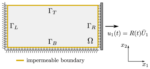
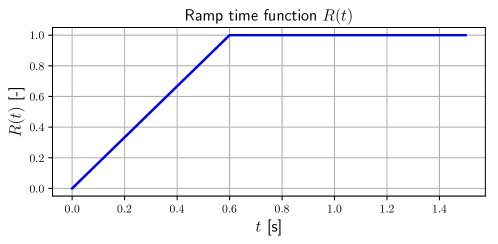
Figure 4: Validation test: top – boundary conditions applied to the macroscopic 2D sample; bottom – ramp function $R(t)$ driving deformations of the macroscopic sample in time.

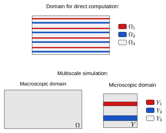
Figure 5: Computational domains: top – domain used in the reference model, build up by repetition ($8\times 4$) of the microscopic unit; bottom – macroscopic domain $\Omega$ (left) and decomposition of microscopic domain $Y$ (right).

	shear modulus	hydraulic permeability
$Y^{l}$	$\mu^{l}$ [MPa]	$\tilde{\boldsymbol{K}}^{l}$ [m2 / (Pa s)]
channel $Y_{1}$	$0.6$	$10^{-6}\boldsymbol{I}$
channel $Y_{2}$	$0.6$	$2\cdot 10^{-6}\boldsymbol{I}$
matrix $Y_{3}$	$1$	$10^{-4}\boldsymbol{I}$

Table 1: Permeability and elasticity parameters in the porous matrix $Y_{3}$ and two channels $Y_{1}$, $Y_{2}$.

The time histories of the pressures in the porous matrix and fluid channel obtained by the reference ($p^{REF}$) and homogenized ($p^{HOM}$) models are compared in Fig. 6. The channel pressure $p_{1}^{HOM}$ is the macroscopic variable involved in system (60), (61), while the matrix pressure $p_{3}^{HOM}$ comes from calculations on the microscopic reference cell, see Algorithm 2. Note that due to the geometry and applied boundary conditions, the computed pressure fields are homogeneous in the matrix and channel parts. The obtained results entitle us to conclude, that the responses of the presented homogenized model are in a close agreement with those of the reference model.

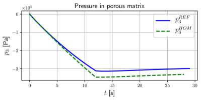
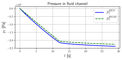
Figure 6: The pressures in the porous matrix and fluid channel obtained by the reference ($p^{REF}$) and homogenized ($p^{HOM}$) models.

5.2 2D shear test

In this and the following section, we demonstrate the proposed two-scale modelling of large deforming porous structures using two simple illustrative simulations.

We consider the macroscopic sample of the same dimensions as in the validation test. The applied boundary conditions, depicted in Fig. 7 left, are as follows: the sample is fixed to the rigid frame at the left boundary ($u_{1}=u_{2}=0$ on $\Gamma_{L}$), the displacement of the right boundary is zero in $x_{1}$-direction ($u_{1}=0$ on $\Gamma_{R}$) and it is driven in time by function $u_{2}(t)=R(t)\bar{U}_{2}$ in $x_{2}$-direction, where $\bar{U}_{2}=-0.08$ m and the ramp function $R(t)$ is defined in 5.1. The reference periodic cell is established by two curved channels embedded in the porous matrix, see Fig. 7 right, with the material parameters defined in Tab. 1. The scaling parameter for the following simulations is $\varepsilon=10^{-3}$.

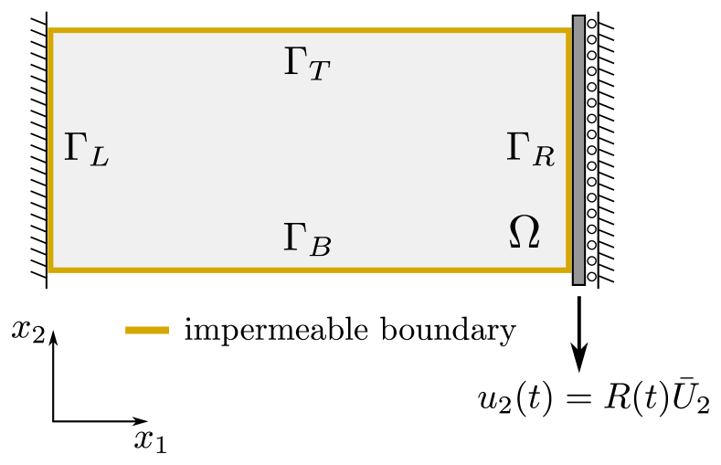
Figure 7: Shear test: left – boundary conditions applied to the macroscopic 2D sample; right – geometry of the microscopic periodic cell.

The resulting macroscopic deformations, pressure distributions, averaged Cauchy stress component $\mathcal{S}_{12}$, the deformed microscopic cells $Y$ and the pressure field $p_{3}$ together with perfusion velocities $w_{3}$ at two selected points $A$, $B$ of domain $\Omega$ are displayed in Fig. 8 for a particular time $t=0.8$ s. In Fig. 9 we show the time evolution of the homogenized coefficients $\boldsymbol{\mathcal{D}}$, $\boldsymbol{\mathcal{B}}^{\alpha}$, $\boldsymbol{\mathcal{C}}^{\alpha}$, $\boldsymbol{\mathcal{Q}}$, $\boldsymbol{\mathcal{S}}$ at a given macroscopic points. The components of the macroscopic deformation gradient $\boldsymbol{F}$ and channel pressures $p^{0}_{\alpha}$ are shown in Fig. 10.

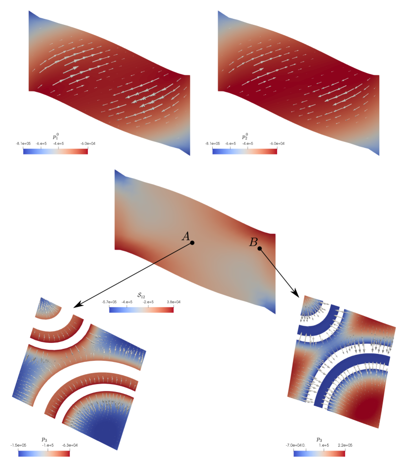
Figure 8: Shear test: top – deformed macroscopic sample at time $t=0.8$ s, pressure fields $p_{1}^{0}$, $p_{2}^{0}$ and the directions of perfusion velocities; middle – magnitude of the averaged Cauchy stress tensor $\boldsymbol{\mathcal{S}}$; bottom – deformed microscopic reference cells at macroscopic points $A$, $B$, reconstructed pressure field $p_{3}$ associated with the solid part $Y_{3}$ and the directions of perfusion velocities at the microscopic level.

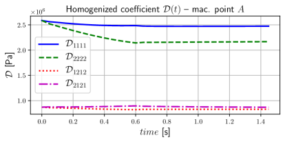
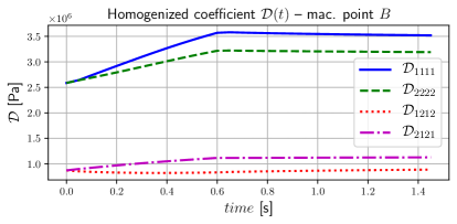
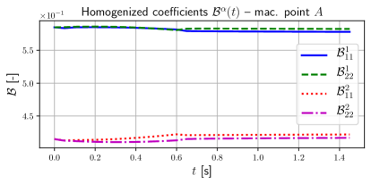
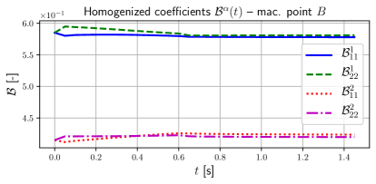
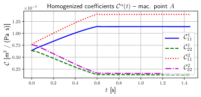
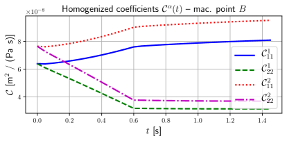
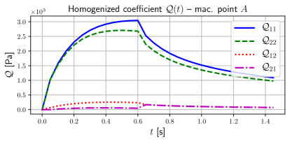
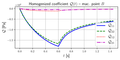
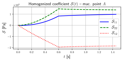
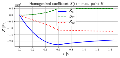
Figure 9: Shear test: time evolution of the homogenized coefficients $\boldsymbol{\mathcal{D}}$, $\boldsymbol{\mathcal{B}}^{\alpha}$, $\boldsymbol{\mathcal{C}}^{\alpha}$, $\boldsymbol{\mathcal{Q}}$, $\boldsymbol{\mathcal{S}}$ at two selected macroscopic points $A$ and $B$.

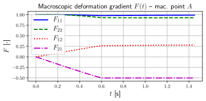
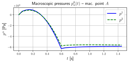
Figure 10: Shear test: left – components of the macroscopic deformation gradient $\boldsymbol{F}$ at point A; right – macroscopic pressures $p^{0}_{\alpha}$ at point A.

5.3 2D inflation test

The same microscopic and macroscopic geometries and the material parameters of the constituents as in the previous example are employed in the simple inflation test presented in this part. The macroscopic sample is attached to the rigid frame at the bottom edge ($u_{1}=u_{2}=0$ on $\Gamma_{B}$) and two prescribed pressures $\bar{P}_{1}=3\cdot 10^{5}$ Pa and $\bar{P}_{2}=1.5\cdot 10^{5}$ Pa multiplied by the ramp functions $R_{\alpha}(t)$ are applied at the left ($\Gamma_{L}$) and right ($\Gamma_{R}$) edges of the sample, see Fig. 11. The part of the boundary where $p_{\alpha}$ is not imposed, is assumed to be impermeable for fluid system $\alpha$, e.i. $\frac{\partial p_{1}}{\partial n}=0$ on $\Gamma\setminus\Gamma_{L}$ and $\frac{\partial p_{2}}{\partial n}=0$ on $\Gamma\setminus\Gamma_{R}$.

Figure 11: Inflation test: left – boundary conditions applied to the macroscopic 2D sample; right – ramp functions $R_{\alpha}(t)$ employed in the pressure boundary conditions.

The macroscopic and microscopic pressures and deformations induced by the prescribed channel pressures are shown in Fig. 12 for time $t=0.8$ s. The time changes of the homogenized coefficients $\boldsymbol{\mathcal{C}}$, $\boldsymbol{\mathcal{S}}$ is depicted in Fig. 13, deformation gradient $\boldsymbol{F}$ and pressures $p^{0}_{\alpha}$ are shown in Fig. 14.

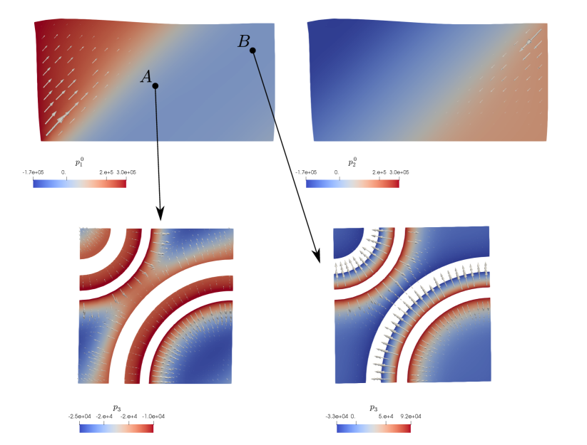
Figure 12: Inflation test: top – deformed macroscopic sample at time $t=0.8$ s, pressure fields $p_{1}^{0}$, $p_{2}^{0}$ and the directions of perfusion velocities; bottom – deformed microscopic reference cells at macroscopic points $A$, $B$, reconstructed pressure field $p_{3}$ associated with the solid part $Y_{3}$ and the directions of perfusion velocities at the microscopic level.

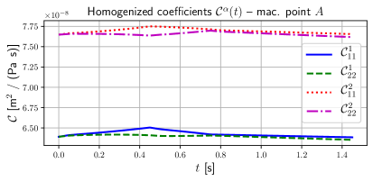
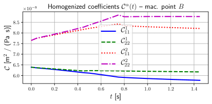
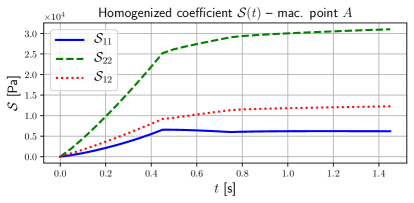
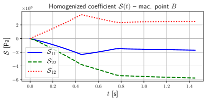
Figure 13: Inflation test: time evolution of the perfusion coefficients $\boldsymbol{\mathcal{C}}^{\alpha}$ and averaged Cauchy stress $\boldsymbol{\mathcal{S}}$ at two selected macroscopic points $A$ and $B$.

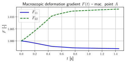
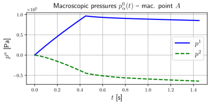
Figure 14: Inflation test: left – components of the macroscopic deformation gradient $\boldsymbol{F}$ at point A; right – macroscopic pressures $p^{0}_{\alpha}$ at point A.

6 Conclusion and outlook

We have proposed the multiscale model of the fluid-saturated porous media undergoing large deformations. Its derivation is based on our previous work [33], where we described modelling of large deforming fluid saturated porous media in the Eulerian framework using a sequential linearization concept for the Biot-type model associated with the deformed configuration.

In this paper, we considered locally periodic heterogeneities featuring the porous medium at the “microscopic” scale which, in reality, may correspond rather to the mesoscopic scale when the multiscale, hierarchical homogenization is in mind. In particular, we considered strong heterogeneities in the permeability to account for the double porosity features of the medium, see e.g. [1, 27, 30, 34, 35, 36], we apply standard homogenization procedures to the linearized equations to derive the two-scale mechanical model of large deforming porous media, assuming a locally periodic microstructure. The proposed two-scale incremental scheme leads to the finite element-square (FE²) computational approach, where local problems and consequently the homogenized properties are calculated by the finite element method in a given points of a macroscopic finite element domain. The coupled computational algorithm has been implemented in the Python based finite element solver SfePy [13], which is suitable for solving various multiscale and multi-physical problems. The homogenization engine, part of SfePy, allows to evaluate all required homogenized coefficients in an efficient way employing parallelization possibilities of a computer system.

The presented 2D numerical examples demonstrate that the proposed two-scale model provides a suitable computational tool for simulating fluid-saturated porous structures with non-linear material behavior under large strains. Due to the special topological arrangement of the microstructure involving two highly permeable channels separated by the dual-porous matrix, this model is supposed to be used in numerical modelling of deforming perfused tissues, such as liver or myocardium, where the microstructural tissue arrangement and embedded vessel networks may considerably affect the mechanical behavior at the organ level. To be able to simulate real structures with complex 3D macroscopic geometries with limited computational power, we need to employ some efficient strategies for reduction of the number of local microscopic problems to be solved. In this respect, various approaches related to this topic has been proposed, see e.g. [24, 20, 39, 17, 18]. These, however, are not directly applicable to the model featured by local internal variables evolving with time, thus, to find a suitable model order reduction remains an important topic for further research.

Appendix A Weak formulation of deformation-diffusion problem

The rate form of the governing equations for the deformation-diffusion problem was derived in [33], where also inertia effects were taken into account, and where a predictor–corrector time integration scheme was proposed. Here, we present the equations without inertia terms and we consider a simple one-step time discretization scheme.

A.1 Rate form of the “force–equilibrium” equation

Substituting (13) and (14) into (12) yields

$$\delta\Phi_{t} ((\boldsymbol{u},p);(\boldsymbol{v},0))\circ(\dot{\boldsymbol{u}},\dot{p},\delta t\mathcal{V})=$$ (62)

$$\int_{\Omega(t)}\Big{[}\nabla\mathcal{V}(\boldsymbol{\sigma}^{\rm eff}-p\boldsymbol{I})+\boldsymbol{\mathbb{D}}^{\rm eff}\boldsymbol{e}(\dot{\boldsymbol{u}})+p\left(\nabla\mathcal{V}+(\nabla\mathcal{V})^{T}\right)-(p\nabla\cdot\mathcal{V}+\dot{p})\boldsymbol{I}\Big{]}:\nabla\boldsymbol{v}$$

$$-\int_{\Omega(t)}\left(\dot{\boldsymbol{f}}\cdot\boldsymbol{v}+\boldsymbol{f}\cdot\boldsymbol{v}\nabla\cdot\mathcal{V}\right)$$

$$= \int_{\Omega(t)}\Big{[}\boldsymbol{\mathbb{D}}^{\rm eff}\boldsymbol{e}(\dot{\boldsymbol{u}})+\nabla\mathcal{V}\boldsymbol{\sigma}^{\rm eff}-p\left((\nabla\cdot\mathcal{V})\boldsymbol{I}-(\nabla\mathcal{V})^{T}\right)-\dot{p}\boldsymbol{I}\Big{]}:\nabla\boldsymbol{v}$$

$$-\int_{\Omega(t)}\left(\dot{\boldsymbol{f}}\cdot\boldsymbol{v}+\boldsymbol{f}\cdot\boldsymbol{v}\nabla\cdot\mathcal{V}\right).$$

Further, we use the time discretization (16), the state increments (10) and, in order to achieve the symmetry of the linearized system, we approximate $\delta t\mathcal{V}$ by the known increment $\delta\boldsymbol{u}^{(k)}$ in terms involving the unknown pressure increment $\delta p^{(k+1)}$ and by $\delta\boldsymbol{u}^{(k+1)}$ in the rest. Thus, we get

$$\delta\Phi_{t} ((\boldsymbol{u}^{(k)},p^{(k)});(\boldsymbol{v},0))\circ(\delta\boldsymbol{u}^{(k+1)},\delta p^{(k+1)},\delta t\mathcal{V})=$$ (63)

$$\int_{\Omega^{(k)}}\boldsymbol{\mathbb{D}}^{\rm eff}\boldsymbol{e}(\delta\boldsymbol{u}^{(k+1)})\boldsymbol{e}(\boldsymbol{v})+\int_{\Omega^{(k)}}\nabla(\delta\boldsymbol{u}^{(k+1)})\boldsymbol{\sigma}^{\rm eff}:\boldsymbol{v}$$

$$-\int_{\Omega^{(k)}}p^{(k)}\left((\nabla\cdot\delta\boldsymbol{u}^{(k+1)})\boldsymbol{I}-(\nabla\delta\boldsymbol{u}^{(k+1)})^{T}\right):\nabla\boldsymbol{v}$$

$$-\int_{\Omega^{(k)}}\Big{[}\delta p^{(k+1)}\left((\nabla\cdot\delta\boldsymbol{u}^{(k)})\boldsymbol{I}-(\nabla\delta\boldsymbol{u}^{(k)})^{T}\right)-\delta p^{(k+1)}\boldsymbol{I}\Big{]}:\nabla\boldsymbol{v}$$

$$-\int_{\Omega^{(k)}}\left(\delta\boldsymbol{f}^{(k+1)}\cdot\boldsymbol{v}+\boldsymbol{f}^{(k)}\cdot\boldsymbol{v}\nabla\cdot\mathcal{V}\right).$$

We add (63) and (7)₁, and due to the residual equation (6), we obtain

$$\int_{\Omega^{(k)}} \Big{[}\boldsymbol{\mathbb{D}}^{\rm eff}\boldsymbol{e}(\delta\boldsymbol{u}^{(k+1)})\boldsymbol{e}(\boldsymbol{v})+\nabla(\delta\boldsymbol{u}^{(k+1)})\boldsymbol{\sigma}^{\rm eff}:\nabla\boldsymbol{v}-p^{(k)}\left((\nabla\cdot\delta\boldsymbol{u}^{(k+1)})\boldsymbol{I}-(\nabla\delta\boldsymbol{u}^{(k+1)})^{T}\right):\nabla\boldsymbol{v}\Big{]}$$ (64)

$$-\int_{\Omega^{(k)}}\delta p^{(k+1)}\left[\left((\nabla\cdot\delta\boldsymbol{u}^{(k)})\boldsymbol{I}-(\nabla\delta\boldsymbol{u}^{(k)})^{T}\right)+\boldsymbol{I}\right]:\nabla\boldsymbol{v}$$

$$=\int_{\Omega^{(k)}}\left(\boldsymbol{f}^{(k+1)}\cdot\boldsymbol{v}-\boldsymbol{\sigma}^{(k)}:\nabla\boldsymbol{v}\right).$$

The expression in the square brackets in the first integral of (64) can be replaced by $\boldsymbol{\mathbb{A}}\boldsymbol{e}(\delta\boldsymbol{u}^{(k+1)})\boldsymbol{e}(\boldsymbol{v})$ using the tangent elastic operator $\boldsymbol{\mathbb{A}}$ introduced in (20). According to (19)₁, expression $\left((\nabla\cdot\delta\boldsymbol{u}^{(k)})\boldsymbol{I}-(\nabla\delta\boldsymbol{u}^{(k)})^{T}\right)$ is equal to $\boldsymbol{B}(\delta\boldsymbol{u}^{(k)})$ and the linearized equilibrium equation attains the following form

$$\int_{\Omega^{(k)}} \boldsymbol{\mathbb{A}}\boldsymbol{e}(\delta\boldsymbol{u}^{(k+1)})\boldsymbol{e}(\boldsymbol{v})-\int_{\Omega^{(k)}}\delta p^{(k+1)}\left(\boldsymbol{B}(\delta\boldsymbol{u}^{(k)})+\boldsymbol{I}\right):\nabla\boldsymbol{v}=\int_{\Omega^{(k)}}\left(\boldsymbol{f}^{(k+1)}\cdot\boldsymbol{v}-\boldsymbol{\sigma}^{(k)}:\nabla\boldsymbol{v}\right).$$ (65)

A.2 Rate form of the “fluid–content” equation

The analogous steps as in A.1 are employed to derive the rate form of the balance of the fluid content. In Eq. (15), the time derivatives are approximated by the finite differences (16), $\delta t\mathcal{V}$ is replaced by $\delta\boldsymbol{u}^{(k)}$ and the state fields $\boldsymbol{u}$, $p$ are rewritten employing the increments defined in (10). Thus, from (15) we get

$$\delta\Phi_{t} ((\boldsymbol{u}^{(k)},p^{(k)});(\boldsymbol{0},q))\circ(\delta\boldsymbol{u}^{(k+1)},\delta p^{(k+1)},\delta t\mathcal{V})=$$ (66)

$$\int_{\Omega(t)}\left(q\nabla\cdot\delta\boldsymbol{u}^{(k+1)}/{\delta t}+\boldsymbol{K}\nabla(p^{(k)}+\delta p^{(k+1)})\cdot\nabla q\right)\nabla\cdot\delta\boldsymbol{u}^{(k)}$$

$$+\int_{\Omega(t)}\left(q\nabla\cdot(\delta\boldsymbol{u}^{(k+1)}-\delta\boldsymbol{u}^{(k)})/\delta t+\boldsymbol{K}\nabla\delta p^{(k+1)}\cdot\nabla q\right)$$

$$-\int_{\Omega(t)}q(\nabla\delta\boldsymbol{u}^{(k)})^{T}:\nabla\delta\boldsymbol{u}^{(k+1)}/\delta t-\int_{\Omega(t)}\boldsymbol{K}\left(\nabla(p^{(k)}+\delta p^{(k+1)})\nabla\delta\boldsymbol{u}^{(k)}\right)\cdot\nabla q$$

$$-\int_{\Omega(t)}\boldsymbol{K}\nabla(p^{(k)}+\delta p^{(k+1)})\cdot\left(\nabla q\nabla\delta\boldsymbol{u}^{(k)}\right)+\int_{\Omega(t)}\delta\boldsymbol{K}\nabla p^{(k)}\cdot\nabla q-\delta\mathcal{J}^{(k+1)}(q)$$

$$= \int_{\Omega(t)}q\left((\nabla\cdot\delta\boldsymbol{u}^{(k)})\boldsymbol{I}-(\nabla\delta\boldsymbol{u}^{(k)})^{T}+\boldsymbol{I}\right):\nabla\delta\boldsymbol{u}^{(k+1)}/{\delta t}-\int_{\Omega(t)}q\nabla\cdot\delta\boldsymbol{u}^{(k)}/\delta t$$

$$+\int_{\Omega(t)}\left(\boldsymbol{K}\nabla\cdot\delta\boldsymbol{u}^{(k)}-(\nabla\delta\boldsymbol{u}^{(k)})\boldsymbol{K}^{T}-\boldsymbol{K}(\nabla\delta\boldsymbol{u}^{(k)})^{T}\right)\nabla(p^{(k)}+\delta p^{(k+1)})\cdot\nabla q$$

$$+\int_{\Omega(t)}\boldsymbol{K}\nabla\delta p^{(k+1)}\cdot\nabla q+\int_{\Omega(t)}\delta\boldsymbol{K}\nabla p^{(k)}\cdot\nabla q-\delta\mathcal{J}^{(k+1)}(q).$$

The time discretization of (7)₂ results in

$$\Phi_{t}((\boldsymbol{u}^{(k)},p^{(k)});(\boldsymbol{0},q))=\int_{\Omega(t)}\left(q\nabla\cdot\delta\boldsymbol{u}^{(k)}/\delta t+\boldsymbol{K}\nabla p^{(k)}\nabla q\right)-\mathcal{J}^{(k)}(q).$$ (67)

By adding (67) to (66) and considering $0=\Phi_{t+\delta t}\approx\Phi_{t}+\delta\Phi_{t}$, see (6) and (8), we obtain the linearized balance equation

$$\int_{\Omega(t)} q\left(\boldsymbol{B}(\delta\boldsymbol{u}^{(k)})+\boldsymbol{I}\right):\nabla\delta\boldsymbol{u}^{(k+1)}/{\delta t}+\int_{\Omega(t)}\left(\boldsymbol{H}(\delta\boldsymbol{u}^{(k)})+\boldsymbol{K}\right)\nabla\delta p^{(k+1)}\cdot\nabla q$$ (68)

$$=\mathcal{J}^{(k+1)}(q)-\int_{\Omega(t)}\left(\boldsymbol{H}(\delta\boldsymbol{u}^{(k)})+\boldsymbol{K}+\delta\boldsymbol{K}\right)\nabla p^{(k)}\cdot\nabla q,$$

where we employed $\boldsymbol{B}(\delta\boldsymbol{u}^{(k)})$ and $\boldsymbol{H}(\delta\boldsymbol{u}^{(k)})$ defined in (19) and $\mathcal{J}^{(k+1)}=\mathcal{J}^{(k)}+\delta\mathcal{J}^{(k+1)}$ contains the new flux at time level $k+1$.

Appendix B

B.1 Symmetric expression for coefficient $\boldsymbol{\mathcal{D}}$

Upon substituting $\boldsymbol{v}=\boldsymbol{\omega}^{ij}$ in (43)₁ and $q=\pi^{kl}$ in (43)₂ summation of the two equations yields the identity

$$a_{Y}\left(\boldsymbol{\omega}^{kl}+\boldsymbol{\Pi}^{kl},\boldsymbol{\omega}^{ij}\right)+b_{Y_{3}}\left(\bar{\boldsymbol{u}};\pi^{kl},\Pi^{ij}\right)+\delta tc_{Y_{3}}\left(\bar{\boldsymbol{u}};\pi^{ij},\pi^{kl}\right)=0,$$ (69)

and hence we get the last equality in (51). However, the minor symmetry does not hold, $\mathcal{D}_{ijkl}\neq\mathcal{D}_{jikl}$, in general, as $\boldsymbol{\omega}^{ij}$ are not symmetric with respect to indices $i,j$, i.e. $\boldsymbol{\omega}^{ij}\neq\boldsymbol{\omega}^{ji}$.

B.2 Equality of coupling coefficients $\boldsymbol{\mathcal{B}}^{\alpha}$ and $\boldsymbol{\mathcal{R}}^{\alpha}$

We shall employ the following identities: From (43)₁ and (44)₂ we get subsequently

$$a_{Y}\left(\boldsymbol{\omega}^{ij},\boldsymbol{\omega}^{\alpha}\right) =-a_{Y}\left(\boldsymbol{\Pi}^{ij},\boldsymbol{\omega}^{\alpha}\right)+b_{Y_{3}}\left(\bar{\boldsymbol{u}};\pi^{ij},\boldsymbol{\omega}^{\alpha}\right)$$ (70)

$$=-a_{Y}\left(\boldsymbol{\Pi}^{ij},\boldsymbol{\omega}^{\alpha}\right)-\delta tc_{Y_{3}}\left(\bar{\boldsymbol{u}};\pi^{\alpha},\pi^{ij}\right).$$

From (44)₁ we have that

$$a_{Y}\left(\boldsymbol{\omega}^{\alpha},\boldsymbol{\omega}^{ij}\right) =b_{Y_{3}}\left(\bar{\boldsymbol{u}};\pi^{\alpha},\boldsymbol{\omega}^{ij}\right)+b_{Y_{\alpha}}\left(\bar{\boldsymbol{u}};1,\boldsymbol{\omega}^{ij}\right).$$ (71)

Further we shall use the strong form of (44)₂; by integrating by parts we obtain

$$\delta t \sum_{\alpha=1,2}\int_{\Gamma_{\alpha}}\left[(\tilde{\boldsymbol{K}}^{3}+\tilde{\boldsymbol{H}}^{3}(\bar{\boldsymbol{u}}))\nabla_{y}\pi^{ij}\right]\cdot\boldsymbol{n}^{3}q\mathrm{\,dS}_{y}-\delta t\int_{Y_{3}}\nabla_{y}\cdot\left[(\tilde{\boldsymbol{K}}^{3}+\tilde{\boldsymbol{H}}^{3}(\bar{\boldsymbol{u}}))\nabla_{y}\pi^{ij}\right]q$$ (72)

$$+b_{Y_{3}}\left(\bar{\boldsymbol{u}};q,\boldsymbol{\omega}^{ij}+\boldsymbol{\Pi}^{ij}\right)=0\quad\forall q\in H_{\#}^{1}(Y_{3}),$$

and hence

$$\nabla_{y}\cdot\left[(\tilde{\boldsymbol{K}}^{3}+\tilde{\boldsymbol{H}}^{3}(\bar{\boldsymbol{u}}))\nabla_{y}\pi^{ij}\right]=(\boldsymbol{B}(\bar{\boldsymbol{u}})+\boldsymbol{I}):\nabla_{y}(\boldsymbol{\omega}^{ij}+\boldsymbol{\Pi}^{ij})\quad\mbox{in }Y_{3}.$$ (73)

On “testing” in (72) by $q=\pi^{\alpha}$ and integrating by parts again,

$$-\delta t\int_{\Gamma_{\alpha}}\left[(\tilde{\boldsymbol{K}}^{3}+\tilde{\boldsymbol{H}}^{3}(\bar{\boldsymbol{u}}))\nabla_{y}\pi^{ij}\right]\cdot\boldsymbol{n}^{3}\mathrm{\,dS}_{y}+\delta tc_{Y_{3}}\left(\bar{\boldsymbol{u}};\pi^{ij},\pi^{\alpha}\right)+b_{Y_{3}}\left(\bar{\boldsymbol{u}};\pi^{\alpha},\boldsymbol{\omega}^{ij}+\boldsymbol{\Pi}^{ij}\right)=0,$$ (74)

and thus

$$-g_{3}^{\alpha}(\bar{\boldsymbol{u}},\pi^{ij})+c_{Y_{3}}\left(\bar{\boldsymbol{u}};\pi^{ij},\pi^{\alpha}\right)+(\delta t)^{-1}b_{Y_{3}}\left(\bar{\boldsymbol{u}};\pi^{\alpha},\boldsymbol{\omega}^{ij}+\boldsymbol{\Pi}^{ij}\right)=0.$$ (75)

Now we can rewrite (56); first we use (71) and (75), which yields

$$\mathcal{R}_{ij}^{\alpha} =|Y|^{-1}b_{Y_{\alpha}}\left(\bar{\boldsymbol{u}};1,\boldsymbol{\omega}^{ij}+\boldsymbol{\Pi}^{ij}\right)+\delta t|Y|^{-1}g_{3}^{\alpha}(\bar{\boldsymbol{u}},\pi^{ij})$$ (76)

$$=|Y|^{-1}\left[b_{Y_{\alpha}}\left(\bar{\boldsymbol{u}};1,\boldsymbol{\Pi}^{ij}\right)+a_{Y}\left(\boldsymbol{\omega}^{\alpha},\boldsymbol{\omega}^{ij}\right)-b_{Y_{3}}\left(\bar{\boldsymbol{u}};\pi^{\alpha},\boldsymbol{\omega}^{ij}\right)\right.$$

$$\quad+\delta t\left.c_{Y_{3}}\left(\bar{\boldsymbol{u}};\pi^{ij},\pi^{\alpha}\right)+b_{Y_{3}}\left(\bar{\boldsymbol{u}};\pi^{\alpha},\boldsymbol{\omega}^{ij}+\boldsymbol{\Pi}^{ij}\right)\right]$$

$$=|Y|^{-1}\left[b_{Y_{\alpha}}\left(\bar{\boldsymbol{u}};1,\boldsymbol{\Pi}^{ij}\right)+a_{Y}\left(\boldsymbol{\omega}^{\alpha},\boldsymbol{\omega}^{ij}\right)\right.$$

$$\quad\left.+\delta tc_{Y_{3}}\left(\bar{\boldsymbol{u}};\pi^{ij},\pi^{\alpha}\right)+b_{Y_{3}}\left(\bar{\boldsymbol{u}};\pi^{\alpha},\boldsymbol{\Pi}^{ij}\right)\right].$$

Then, using (70), we get

$$\mathcal{R}_{ij}^{\alpha} =|Y|^{-1}\left[b_{Y_{\alpha}}\left(\bar{\boldsymbol{u}};1,\boldsymbol{\Pi}^{ij}\right)+b_{Y_{3}}\left(\bar{\boldsymbol{u}};\pi^{\alpha},\boldsymbol{\Pi}^{ij}\right)-a_{Y}\left(\boldsymbol{\Pi}^{ij},\boldsymbol{\omega}^{\alpha}\right)\right]=\mathcal{B}_{ij}^{\alpha},$$ (77)

which is the desired identity.

References

- [1] T. Arbogast, J. Douglas, and U. Hornung. Derivation of the double porosity model of single phase flow via homogenization theory. SIAM Journal on Mathematical Analysis, 21:823–836, 1990.
- [2] J.L. Auriault, C. Boutin, and C. Geindreau. Homogenization of Coupled Phenomena in Heterogenous Media. ISTE. Wiley, 2010.
- [3] A. Bedford and D. S. Drumheller. Theories of immiscible and structured mixtures. International Journal of Engineering Science, 21(8):863–960, 1983.
- [4] A. Bensoussan, J.L. Lions, and G. Papanicolau. Asymptotic Analysis for Periodic Structures. Elsevier Science, 1978.
- [5] M. A. Biot. General theory of three-dimensional consolidation. Journal of Applied Physics, 12(2):155–164, 1941.
- [6] M. A. Biot. Theory of elasticity and consolidation for a porous anisotropic solid. Journal of Applied Physics, 26(2):182–185, 1955.
- [7] R. M. Bowen. Part I - Theory of mixtures. In Continuum Physics, pages 1–127. Academic Press, 1976.
- [8] R. M. Bowen. Compressible porous media models by use of the theory of mixtures. International Journal of Engineering Science, 20(6):697–735, 1982.
- [9] D. L. Brown, Y. Efendiev, and V. H. Hoang. An efficient hierarchical multiscale finite element method for stokes equations in slowly varying media. Multiscale Modeling & Simulation, 11(1):30–58, 2013.
- [10] D. L. Brown, P. Popov, and Y. Efendiev. On homogenization of stokes flow in slowly varying media with applications to fluid-structure interaction. GEM - International Journal on Geomathematics 2, 2(281), 2011.
- [11] D. L. Brown, P. Popov, and Y. Efendiev. Effective equations for fluid-structure interaction with applications to poroelasticity. Applicable Analysis, 93(4):771–790, 2013.
- [12] R. Burridge and J.B. Keller. Biot’s poroelasticity equations by homogenization. In R. Burridge, S. Childress, and G. Papanicolaou, editors, Macroscopic Properties of Disordered Media, pages 51–57. Springer Berlin Heidelberg, 1982.
- [13] R. Cimrman, V. Lukeš, and E. Rohan. Multiscale finite element calculations in Python using Sfepy. Advances in Computational Mathematics, 45(4):1897–1921, 2019.
- [14] D. Cioranescu, A. Damlamian, and G. Griso. The periodic unfolding method in homogenization. SIAM Journal on Mathematical Analysis, 40(4):1585–1620, 2008.
- [15] D. Cioranescu, A. Damlamian, and G. Griso. The Periodic Unfolding Method; Theory and Applications to Partial Differential Problems. Series in Contemporary Mathematics 3. Springer, 2018.
- [16] M. A. Crisfield. Non-linear finite element analysis of solids and structures. Wiley, 1991.
- [17] G. J. Dvorak, Y. A. Bahei-El-Din, and A. M. Wafa. The modeling of inelastic composite materials with the transformation field analysis. Modelling and Simulation in Materials Science and Engineering, 2(3 A):571–586, 1994.
- [18] B. Eidel, A. Fischer, and A. Gote. A Nonlinear Finite Element Heterogeneous Multiscale Method for the Homogenization of Hyperelastic Solids and a Novel Staggered Two-Scale Solution Algorithm. arXiv e-prints, page arXiv:1908.08292, Aug 2019.
- [19] F. Feyel. A multilevel finite element method (fe2) to describe the response of highly non-linear structures using generalized continua. Computer Methods in Applied Mechanics and Engineering, 192(28):3233–3244, 2003.
- [20] F. Fritzen and M. Leuschner. Reduced basis hybrid computational homogenization based on a mixed incremental formulation. Computer Methods in Applied Mechanics and Engineering, 260:143–154, 2013.
- [21] S. J. Hollister, J. M. Brennan, and N. Kikuchi. A homogenization sampling procedure for calculating trabecular bone effective stiffness and tissue level stress. Journal of Biomechanics, 27(4):433–444, 1994.
- [22] S. V. Lomov, E. Bernal, D. S. Ivanov, S. V. Kondratiev, and I. Verpoest. Homogenisation of a sheared unit cell of textile composites. Revue Européenne des Éléments Finis, 14(6-7):709–728, 2005.
- [23] V. Lukeš and E. Rohan. Microstructure based two-scale modelling of soft tissues. Mathematics and Computers in Simulation, 80(6):1289 – 1301, 2010.
- [24] J. C. Michel and P. Suquet. Nonuniform transformation field analysis. International Journal of Solids and Structures, 40(25):6937–6955, 2003.
- [25] C. Miehe, J. Dettmar, and D. Zäh. Homogenization and two-scale simulations of granular materials for different microstructural constraints. International Journal for Numerical Methods in Engineering, 83:1206–1236, 2010.
- [26] I. Özdemir, W.A.M. Brekelmans, and M.G.D. Geers. Fe2 computational homogenization for the thermo-mechanical analysis of heterogeneous solids. Computer Methods in Applied Mechanics and Engineering, 198(3):602–613, 2008.
- [27] S.R. Pride and J.G. Berryman. Linear dynamics of double-porosity dual-permeability materials. II. fluid transport equations. Physical Review E - Statistical Physics, Plasmas, Fluids, and Related Interdisciplinary Topics, 68(3):10, 2003.
- [28] M. Ptashnyk. Locally periodic unfolding method and two-scale convergence on surfaces of locally periodic microstructures. Multiscale Modeling and Simulation, 13(3):1061–1105, 2015.
- [29] A. Ramírez-Torres, R. Penta, R. Rodríguez-Ramos, and A. Grillo. Effective properties of hierarchical fiber-reinforced composites via a three-scale asymptotic homogenization approach. Mathematics and Mechanics of Solids, pages 3554–3574, 2019.
- [30] E. Rohan and R. Cimrman. Two-scale modelling of tissue perfusion problem using homogenization of dual prous media. International Journal for Multiscale Computational Engineering, 8:81–102, 2010.
- [31] E. Rohan, R. Cimrman, and V. Lukeš. Numerical modelling and homogenized constitutive law of large deforming fluid saturated heterogeneous solids. Computers & Structures, 84(17):1095–1114, 2006.
- [32] E. Rohan and V. Lukeš. On modelling nonlinear phenomena in deforming heterogeneous media using homogenization and sensitivity analysis concepts. Applied Mathematics and Computation, 267:583–595, 2015.
- [33] E. Rohan and V. Lukeš. Modeling large-deforming fluid-saturated porous media using an Eulerian incremental formulation. Advances in Engineering Software, 113:84–95, 2017.
- [34] E. Rohan, S. Naili, R. Cimrman, and T. Lemaire. Multiscale modeling of a fluid saturated medium with double porosity: Relevance to the compact bone. Journal of the Mechanics and Physics of Solids, 60(5):857–881, 2012.
- [35] E. Rohan, S. Naili, and V.-H. Nguyen. Modelling of waves in fluid-saturated porous media with high contrast heterogeneity: homogenization approach. ZAMM - Journal of Applied Mathematics and Mechanics / Zeitschrift für Angewandte Mathematik und Mechanik, 98(9):1699–1733, 2018.
- [36] Eduard Rohan, Vu-Hieu Nguyen, and Salah Naili. Numerical modelling of waves in double-porosity biot medium. Computers & Structures, 232:105849, 2020. Mechanics and Modelling of Materials and Structures.
- [37] E. Sanchez-Palencia. Non-homogeneous media and vibration theory. Number 127 in Lecture Notes in Physics. Springer, Berlin, 1980.
- [38] J. Schröder. A numerical two-scale homogenization scheme: the FE2-method, pages 1–64. Springer Vienna, Vienna, 2014.
- [39] V. Sepe, S. Marfia, and E. Sacco. A nonuniform TFA homogenization technique based on piecewise interpolation functions of the inelastic field. Internation Journal of Solids and Structures, 50(5):725–742, 2013.
- [40] T. L. Van Noorden and A. Muntean. Homogenisation of a locally periodic medium with areas of low and high diffusivity. European Journal of Applied Mathematics, 22(5):493–516, 2011.
- [41] S. Whitaker. The method of volume averaging, volume 13 of Theory and Applications of Transport in Porous Media. Springer, 1999.
- [42] J. Yvonnet. Computational Homogenization of Heterogeneous Materials with Finite Elements. Springer International Publishing, 2019.
- [43] J. Yvonnet and Q.-C. He. The reduced model multiscale method (R3M) for the non-linear homogenization of hyperelastic media at finite strains. Journal of Computational Physics, 223(1):341–368, 2007.
- [44] J. Zeman, J. Novák, M. Šejnoha, and J. Šejnoha. Pragmatic multi-scale and multi-physics analysis of Charles bridge in Prague. Engineering Structures, 30(11):3365–3376, 2008.