Non-Asymptotic Performance Analysis of Size-Based Routing Policies

Abstract

We investigate the performance of two size-based routing policies: the Size Interval Task Assignment (SITA) and Task Assignment based on Guessing Size (TAGS). We consider a system with two servers and Bounded Pareto distributed job sizes with tail parameter 1 where the difference between the size of the largest and the smallest job is finite. We show that the ratio between the mean waiting time of TAGS over the mean waiting time of SITA is unbounded when the largest job size is large and the arrival rate times the largest job size is less than one. We provide numerical experiments that show that our theoretical findings extend to Bounded Pareto distributed job sizes with tail parameter different to $1$.

I Introduction

Figure 1: A system operating under the TAGS policy

Figure 2: A system operating under the SITA policy

Many existing routing policies to parallel queues are included in the SQ(d) framework, where for each incoming job, $d\geq 2$ servers are picked uniformly at random to observe their states and the job is routed to the server in the best state among the observed ones. It is known that the performance of this kind of systems is very good (see [1, 2, 3, 4]), however the author in [5] showed that when the variability of the job size distribution is high this family of policies are not optimal. This is, in fact, the regime where the size-based routing policies outperform the routing policies that belong the SQ(d) family of policies.

In this work, we study two size-based policies: the Size Interval Task Assignment (SITA) [6] and the Task Assignment with Guessing Size (TAGS) [7]. In the former policy, short jobs and long jobs are executed in different servers and, therefore, it is assumed that the size of incoming tasks is known. In the latter policy, all the jobs are executed in one server and, if a job does not end its service before a given deadline, it is stopped and enqueued in the other server, where it starts service from scratch. From the above definitions, it follows clearly that the mean waiting time of jobs in the SITA system is smaller than in the TAGS system. Recently, the authors in [8, 9] show for Bounded Pareto distributed job sizes that, when the difference between the smallest and the largest job size tends to infinity and the total load of the system is less than one, the ratio of the mean waiting time of TAGS over the mean waiting time of SITA is upper bounded by 2.

We consider a system with two servers and we compare the mean waiting time of both systems in a non-asymptotic regime where the difference between the size of the largest and the smallest job is finite. We show that the ratio of the mean waiting time of the TAGS system over that of the SITA system is unbounded for the Bounded Pareto distribution with tail parameter $1$ when the largest job size is large and the arrival rate times the largest job size is less than one. Our numerical experiments show that the performance ratio of both systems is unbounded other values of the tail parameter of the Bounded Pareto distribution and it can be large even if the arrival rate is not small.

II Model Description

II-A Notation

We consider a system with two servers with equal capacity. We assume that the servers are FCFS queues. Arriving jobs follow a Poisson distribution with rate $\lambda$. The size of the jobs is given by a sequence of i.i.d. random variables denoted by $X$. We denote by $F(s)=\mathbb{P}[X<s]$ the cumulative distribution function of the job size distribution. We assume $F(\cdot)$ to be differentiable and we write $f(s)=\frac{dF(s)}{ds}$. We assume that the size of the smallest job is one and the size of the largest job is $r>1$. The load of the system is denoted by $\rho$ and to ensure stability we assume that $\rho<1$.

II-B The TAGS System

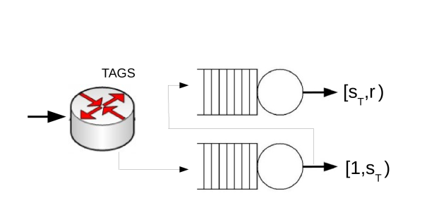
We focus on the TAGS routing (see Figure 2). Let $s\in[1,r].$ In this policy, all incoming jobs are sent to Server $1$. If a job has been served before $s$ units of time in Server 1, it leaves the system; otherwise, when the execution time equals $s$, it is stopped and sent to the end of the queue of Server 2, where the execution starts from scratch. Jobs that are executed in Server 2 are always executed until completion.

For a given value $s$, we denote by $W^{TAGS}(s)$ the random variable of the waiting time of incoming jobs under TAGS policy. We define as $s_{T}$ the value of $s$ such that the mean waiting time of the TAGS system is minimized, i.e.,

$$s_{T}=\operatorname*{arg\,min}_{s}\mathbb{E}[W^{TAGS}(s)].$$

From the above description, it follows that

$$\mathbb{E}[W^{TAGS}(s_{T})]= \mathbb{E}[W_{1}^{TAGS}(s_{T})]$$

$$+\left(\int_{s_{T}}^{r}f(x)dx\right)s_{T}$$

$$+\left(\int_{s_{T}}^{r}f(x)dx\right)\mathbb{E}[W_{2}^{TAGS}(s_{T})],$$ (1)

where $\mathbb{E}[W_{i}^{TAGS}(s_{T})]$ is the mean waiting time of jobs in Server $i$ when the threshold value is $s_{T}$.

II-C The SITA System

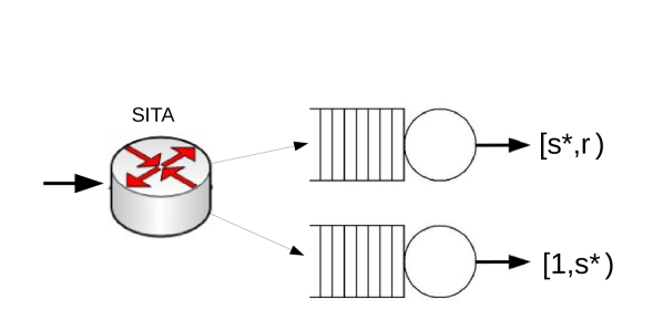
We focus on the SITA routing (see Figure 2). This policy assumes that the size of incoming jobs is known [10, 11]. Let $s\in[1,r].$ Under the SITA policy with cutoff $s$, jobs whose size is smaller than $s$ are sent to Server 1, whereas jobs whose size is larger than $s$ to Server 2. The random variable of the waiting time of incoming jobs under the SITA policy with cutoff $s$ is denoted by $W^{SITA}(s)$. We define as $s^{*}$ the value of $s$ such that the mean waiting time of the SITA system is minimized, i.e.,

$$s^{*}=\operatorname*{arg\,min}_{s}\mathbb{E}[W^{SITA}(s)].$$

The mean waiting time of jobs under the SITA policy with cutoff $s^{*}$ is given by

$$\mathbb{E}[W^{SITA}(s^{*})] =\left(\int_{1}^{s^{*}}f(x)dx\right)\mathbb{E}[W_{1}^{SITA}(s^{*})]$$

$$+\left(\int_{s^{*}}^{r}f(x)dx\right)\mathbb{E}[W_{2}^{SITA}(s^{*})],$$ (2)

where $\mathbb{E}[W_{i}^{SITA}(s^{*})]$ is the mean waiting time of jobs in Server $i$.

II-D The Bounded Pareto Distribution

We now present the Bounded Pareto distribution. A distribution $X$ is said to be Bounded Pareto with parameters $1$, $r$ and $\alpha$ if its density has the following form: if $1\leq x\leq r$, then

$$f(x)=\frac{\alpha x^{-\alpha-1}}{(1-(1/r)^{\alpha})},$$

and $f(x)=0$ otherwise. Besides, the cumulative distribution function of the Bounded Pareto distribution is given by the following expression:

$$F(x)=\begin{cases}0,&x\leq 1,\\ \frac{1-(1/x)^{\alpha}}{1-(1/r)^{\alpha}},&1\leq x\leq r,\\ 1,&x\geq r.\end{cases}$$

Besides, when $\alpha\neq 1$, we have that the mean of the distribution is given by $\frac{\alpha}{\alpha-1}\frac{1-(1/r)^{\alpha-1}}{1-(1/r)^{\alpha}}$whereas when $\alpha=1$ $\frac{\ln(r)}{1-\frac{1}{r}}.$The Bounded Pareto distribution with large range and $0<\alpha<2$ is know to be a good model for high variance job size distributions [12]. We also note that the Bounded Pareto distribution with $\alpha=-1$ coincides with the uniform distribution on the interval $[1,r]$. Besides, the most favorable distribution of SITA and TAGS is given when $\alpha=1$ [8]. This is, indeed, the case we study in the next section.

III Bounded Pareto Distribution with $\alpha=1$

We consider the Bounded Pareto distribution with $\alpha=1$ and we aim to compare the mean waiting time of a system with two queues operating under the TAGS routing with that of a system with two queues operating under the SITA routing. In the following result, we provide a lower-bound of the performance of the TAGS system.

Lemma 1.

For the Bounded Pareto distribution with $\alpha=1$, if $\lambda r<1$,

$$\mathbb{E}[W^{TAGS}(s_{T})]>\lambda r.$$

Proof.

We aim to study the optimal performance of the TAGS system with two queues. It follows from (1) that

$$\mathbb{E}[W^{TAGS}(s_{T})]\geq \mathbb{E}[W_{1}^{TAGS}(s_{T})]$$

$$+\left(\int_{s_{T}}^{r}f(x)dx\right)s_{T}.$$

For the Bounded Pareto distribution with $\alpha=1$, we have that

$$\mathbb{E}[W_{1}^{TAGS}(s_{T})]+\left(\int_{s_{T}}^{r}f(x)dx\right)s_{T}=$$

$$\frac{\lambda(s_{T}-1)}{2(1-\rho)(1-\tfrac{1}{r})}+\frac{1-\tfrac{s_{T}}{r}}{1-\tfrac{1}{r}}\geq$$

$$\frac{\lambda(s_{T}-1)}{2(1-\tfrac{1}{r})}+\frac{1-\tfrac{s_{T}}{r}}{1-\tfrac{1}{r}}=\frac{s_{T}(\lambda-\tfrac{1}{r})+2-2\lambda}{2(1-\tfrac{1}{r})}.$$

If $\lambda r<1$, then $\frac{x(\lambda-\tfrac{1}{r})+2-2\lambda}{2(1-\tfrac{1}{r})}$ decreases with $x$. Thus,

$$\frac{s_{T}(\lambda-\tfrac{1}{r})+2-2\lambda}{2(1-\tfrac{1}{r})} \geq\frac{r(\lambda-\tfrac{1}{r})+2-2\lambda}{2(1-\tfrac{1}{r})}$$

$$=\frac{\lambda(r-2)+1}{2(1-\tfrac{1}{r})}>\frac{\lambda(r-2)+\lambda r}{2(1-\tfrac{1}{r})}=\lambda r.$$

∎

It is important to note that, unlike in the previous work [8], we do not need to assume Poisson arrivals to all the servers in the above result. In the following result, we characterize the mean waiting time of the SITA system.

Lemma 2.

For the Bounded Pareto distribution with $\alpha=1$, when $\lambda r<1$ and $r$ is large,

$$\mathbb{E}[W^{SITA}(s^{*})]\leq\frac{\lambda(\sqrt{r}-1)^{2}}{\sqrt{r}(1-\tfrac{1}{r})^{2}}.$$

Proof.

We first note that the load of each server is upper bounded by $\rho$. Therefore, for the Bounded Pareto distribution with $\alpha=1$, we have that

$$\mathbb{E}[W_{1}^{SITA}(s^{*})]\leq\frac{\lambda(s^{*}-1)}{2(1-\rho)(1-(1/r))}$$

and

$$\mathbb{E}[W_{2}^{SITA}(s^{*})]\leq\frac{\lambda(r-s^{*})}{2(1-\rho)(1-(1/r))},$$

where $\rho=\lambda\ln(r)$. We now note that,

$$\lambda r<1\iff\lambda\ln(r)<\frac{ln(r)}{r}.$$

Since when $r$ is large, $\frac{\ln(r)}{r}$ tends to zero and $\rho=\lambda\ln(r)$, it follows that $\rho$ tends to zero when $\lambda r<1$. As a result,

$$\mathbb{E}[W_{1}^{SITA}(s^{*})]\leq\frac{\lambda(s^{*}-1)}{2(1-(1/r))}$$

and

$$\mathbb{E}[W_{2}^{SITA}(s^{*})]\leq\frac{\lambda(r-s^{*})}{2(1-(1/r))}.$$

We know from Section 3.2.4 of [13] that, for the Bounded Pareto distribution with $\alpha=1$, $s^{*}$ balances the load of both servers and, therefore, it can be obtained as follows:

$$\int_{1}^{s^{*}}f(x)dx=\int_{s^{*}}^{r}f(x)dx\iff s^{*}=\sqrt{r}.$$

As a result,

$$\mathbb{E}[W_{1}^{SITA}(s^{*})]\leq\frac{\lambda(\sqrt{r}-1)}{2(1-(1/r))}$$

and

$$\mathbb{E}[W_{2}^{SITA}(s^{*})]\leq\frac{\lambda(r-\sqrt{r})}{2(1-(1/r))}.$$

Therefore, from (2), it follows that

$$\mathbb{E}[W^{SITA}(s^{*})] \leq\left(\int_{1}^{s^{*}}f(x)dx\right)\frac{\lambda(\sqrt{r}-1)}{2(1-(1/r))}$$

$$+\left(\int_{s^{*}}^{r}f(x)dx\right)\frac{\lambda(r-\sqrt{r})}{2(1-(1/r))}$$

$$=\left(\int_{1}^{\sqrt{r}}f(x)dx\right)\frac{\lambda(\sqrt{r}-1)}{2(1-(1/r))}$$

$$+\left(\int_{\sqrt{r}}^{r}f(x)dx\right)\frac{\lambda(r-\sqrt{r})}{2(1-(1/r))}$$

$$=\frac{\lambda(1-\tfrac{1}{\sqrt{r}})(\sqrt{r}-1)}{2(1-(1/r))^{2}}$$

$$+\frac{\lambda(\tfrac{1}{\sqrt{r}}-\tfrac{1}{r})(r-\sqrt{r})}{2(1-(1/r))^{2}}$$

$$=\frac{\lambda(\tfrac{1}{\sqrt{r}}-\tfrac{1}{r})(r-\sqrt{r})}{(1-(1/r))^{2}}$$

$$=\frac{\lambda(\sqrt{r}-1)^{2}}{\sqrt{r}(1-(1/r))^{2}}.$$

∎

From the above lemmas, we have that when $\lambda r<1$ and $r$ is large, the ratio between the mean waiting time of TAGS over the mean waiting time of SITA is lower bounded by

$$\frac{\lambda r}{\frac{\lambda(\sqrt{r}-1)^{2}}{\sqrt{r}(1-(1/r))^{2}}}=\frac{(\sqrt{r}+1)^{2}}{\sqrt{r}},$$

where the equality is obtained by simplifying the derived expression. Interestingly, the last expression does not depend on $\lambda$. Besides, we now show that it is increasing with $r$.

Lemma 3.

The function $\frac{(\sqrt{r}+1)^{2}}{\sqrt{r}}$ is increasing with $r$.

Proof.

We aim to show that $\frac{(\sqrt{r}+1)^{2}}{\sqrt{r}}$ is increasing with $r$, which is true if and only if

$$((\sqrt{r}+1)^{2})^{\prime}\sqrt{r}-(\sqrt{r})^{\prime}(\sqrt{r}+1)^{2}>0\iff$$

$$\frac{2(\sqrt{r}+1)}{2\sqrt{r}}\sqrt{r}-\frac{1}{2\sqrt{r}}(\sqrt{r}+1)^{2}>0\iff$$

$$\sqrt{r}+1-\frac{1}{2\sqrt{r}}(\sqrt{r}+1)^{2}>0\iff$$

$$1-\frac{1}{2\sqrt{r}}(\sqrt{r}+1)>0\iff$$

$$2\sqrt{r}-(\sqrt{r}+1)>0\iff\sqrt{r}-1>0$$

∎

From the above results and using that $\frac{(\sqrt{r}+1)^{2}}{\sqrt{r}}$ tends to infinity when $r\to\infty$, it follows that when $\lambda r<1$, the ratio between the mean waiting time of the TAGS system and the mean waiting time of the SITA system is lower bounded by a function that is unbounded and the following result follows.

Theorem 4.

The ratio of the mean waiting time of the TAGS system and the mean waiting time of the SITA system is unbonded.

IV Numerical Experiments

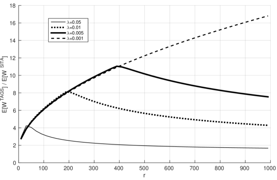
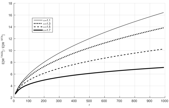
We present our numerical work, which focuses on the ratio between the mean waiting time of the TAGS system and the mean waiting time of the SITA system for the Bounded Pareto distribution. We investigate the evolution of this ratio when we vary $r$ from $10$ to $1000$ for different values of $\lambda$ and different values of $\alpha$. In Figure 3, we consider that $\alpha=1$ and we depict the ratio between the mean waiting time of the TAGS system and the mean waiting time of the SITA system as a function of $r$ for different values of $\lambda$. We observe that the maximum of this ratio is 4 when $\lambda=0.05$, 8 when $\lambda=0.01$, $11$ when $\lambda=0.005$ and when $\lambda=0.001$ the performance ratio is increasing with $r$ for the considered values of $r$. This illustration shows that the maximum over $r$ of the performance ratio under consideration increases when we decrease $\lambda$ and also that it can be large even if the value of the arrival rate is not very small. In Figure 4, we consider an arrival rate of $0.001$ and we study the evolution of the ratio between the mean waiting time of the TAGS system and the mean waiting time of the SITA system over $r$ for several values of $\alpha$ larger than one. We observe that the performance ratio under study is increasing with $r$ for the considered values of $r$. Similar results have been obtained for this performance ratio for different values of $\alpha$ which are smaller than one, that is, ratio between the mean waiting time of TAGS and the mean waiting time of SITA is also increasing with $r$ when $\alpha$ is smaller than 1. We omit this illustration due to lack of space.

Figure 3: The ratio $\mathbb{E}[W^{TAGS}(s_{T})]/\mathbb{E}[W^{SITA}(s_{T})]$ as a function of $r$ for different values of $\lambda$.

Figure 4: The ratio $\mathbb{E}[W^{TAGS}(s_{T})]/\mathbb{E}[W^{SITA}(s_{T})]$ as a function of $r$ for different values of $\alpha$.

References

- [1] R. D. Foley, D. R. McDonald et al., “Join the shortest queue: stability and exact asymptotics,” The Annals of Applied Probability, vol. 11, no. 3, pp. 569–607, 2001.
- [2] R. R. Weber, “On the optimal assignment of customers to parallel servers,” Journal of Applied Probab., vol. 15, no. 2, pp. 406–413, 1978.
- [3] A. W. Richa, M. Mitzenmacher, and R. Sitaraman, “The power of two random choices: A survey of techniques and results,” Combinatorial Optimization, vol. 9, pp. 255–304, 2001.
- [4] W. Winston, “Optimality of the shortest line discipline,” Journal of Applied Probability, vol. 14, no. 1, pp. 181–189, 1977.
- [5] W. Whitt, “Deciding which queue to join: Some counterexamples,” Operations Research, vol. 34, no. 1.
- [6] M. Harchol-Balter, M. E. Crovella, and C. D. Murta, “On choosing a task assignment policy for a distributed server system,” Journal of Parallel and Distributed Computing, vol. 59, no. 2, pp. 204–228, 1999.
- [7] M. Harchol-Balter, “Task assignment with unknown duration,” in Proceedings 20th IEEE International Conference on Distributed Computing Systems. IEEE, 2000, pp. 214–224.
- [8] E. Bachmat, J. Doncel, and H. Sarfati, “Performance and stability analysis of the task assignment based on guessing size routing policy,” IEEE 27th International Symposium on Modeling, Analysis, and Simulation of Computer and Telecommunication Systems, pp. 1–13, 2019.
- [9] ——, “Analysis of the task assignment based on guessing size policy,” Performance Evaluation, vol. 142, p. 102122, 2020.
- [10] J. Doncel, S. Aalto, and U. Ayesta, “Performance degradation in parallel-server systems,” IEEE/ACM Trans. on Netw., vol. 27, no. 2, pp. 875–888, April 2019.
- [11] J. Anselmi and J. Doncel, “Asymptotically optimal size-interval task assignments,” IEEE Transactions on Parallel and Distributed Systems, vol. 30, no. 11, pp. 2422–2433, 2019.
- [12] M. Harchol-Balter and A. B. Downey, “Exploiting process lifetime distributions for dynamic load balancing,” ACM Trans. Comput. Syst., vol. 15, no. 3, pp. 253–285, Aug. 1997.
- [13] M. Harchol-Balter and R. Vesilo, “To balance or unbalance load in size-interval task allocation,” Probability in the Engineering and Informational Sciences, vol. 24, no. 2, pp. 219–244, 2010.