Ada-Segment: Automated Multi-loss Adaptation for Panoptic Segmentation

Abstract

Panoptic segmentation that unifies instance segmentation and semantic segmentation has recently attracted increasing attention. While most existing methods focus on designing novel architectures, we steer toward a different perspective: performing automated multi-loss adaptation (named Ada-Segment) on the fly to flexibly adjust multiple training losses over the course of training using a controller trained to capture the learning dynamics. This offers a few advantages: it bypasses manual tuning of the sensitive loss combination, a decisive factor for panoptic segmentation; it allows to explicitly model the learning dynamics, and reconcile the learning of multiple objectives (up to ten in our experiments); with an end-to-end architecture, it generalizes to different datasets without the need of re-tuning hyperparameters or re-adjusting the training process laboriously. Our Ada-Segment brings 2.7% panoptic quality (PQ) improvement on COCO val split from the vanilla baseline, achieving the state-of-the-art $48.5\%$ PQ on COCO test-dev split and 32.9% PQ on ADE20K dataset. The extensive ablation studies reveal the ever-changing dynamics throughout the training process, necessitating the incorporation of an automated and adaptive learning strategy as presented in this paper.

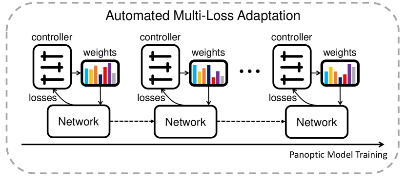
Figure 1: Our Ada-Segment aims at automatically adjusting the weights of multiple objectives in panoptic segmentation during training for achieving the balanced learning dynamics, in contrast to existing works that rely on carefully hand-tuned weights after tediously re-training multiple times. It adjusts the training loss every training epochs on the fly via a weight controller within a single training procedure. Ada-Segment can achieve remarkably better results than results without loss tuning and also perform significant better than other hyperparameter tuning methods.

Introduction

Capitalized on advances from traditional semantic segmentation and instance segmentation, the vision community recently steps forward to resolve a more challenging task, panoptic segmentation (Kirillov et al. 2018), which targets at simultaneously segmenting both foreground instance things (e.g., person, car and dog) and background semantic stuff (e.g., sky, river and sea), achieving a more unified understanding of images. Hence, panoptic segmentation is usually formulated as a multi-objective problem for jointly optimizing for semantic and instance segmentation. To solve this problem, many existing methods (Kirillov et al. 2019; Xiong et al. 2019; Porzi et al. 2019; Chen et al. 2019) have designed multi-branched network architectures, while each branch mapping to an instance or semantic segmentation objective and resulted in many (up to ten in our experiments) individual losses that need to be reconciled during training.

Various network modules or fusing strategies (Kirillov et al. 2019; Xiong et al. 2019; Liu et al. 2019; Lazarow et al. 2020) have been proposed to deal with the consistency of learning or predictions from instance segmentation and semantic segmentation branches. As reported in many literatures (Kirillov et al. 2019; Xiong et al. 2019), the performance of a panoptic segmentation architecture exhibits extreme sensitivity and variability

with respect to the multi-objective loss weights. Therefore, previous works relied on exhaustive hyper-parameter search over such weights. For example, Panoptic FPN (Kirillov et al. 2019) uses a grid search to find better loss weights on two datasets; UPSNet (Xiong et al. 2019) carefully investigates the weighting scheme of loss functions. In our experiments, different loss weights may yield 2% performance difference (measured in PQ). It is thus hard to disentangle the advantages of an improved method from a better hyperparameter setting.

Moreover, previous works only apply static loss weights throughout the training, skipping chances for the appropriate adaptation to the dynamically-varying convergence behaviors, as observed in our experiments. Finally, hand-tuned loss weights, whenever changing to a different dataset, must be carefully re-tuned, prohibiting the generalization across different data distributions.

To address these limitations, we present Ada-Segement, an efficient automated multi-loss adaptation framework to dynamically adjust the loss weight with respect to each sub-objective, seeking an improved optimization schedule during training. In Figure 1, Ada-Segment introduces an end-to-end weight controller to automatically generate loss weights to adjust model’s training loss. Departing from fixing a group of static weights during training, Ada-Segment adjusts the loss weights based on the training conditions with the weight controller. Specifically, the weight controller is firstly trained with several models training in parallel. It gathers training information from all models after a few training iterations (e.g., an epoch) and produces new weights for training. Besides, we find the trained controller is of the capability to capture the ever-changing training dynamics so that we can directly re-use it to automatically adjust training loss when training models on different datasets, training schedules and backbone networks.

Our main contributions are summarized as follows: (1) We propose Ada-Segment as a framework to automatically balance the multiple objectives in panotpic segmentation, bypassing tedious manual tuning of loss combination weights. (2) We introduce a novel weight controller within the multi-loss adaptation strategy that can capture the learning dynamics to adjust the loss weights during training, which is of the capability to transfer between different backbone network, training schedule and datasets. 3) We empirically demonstrate the significance of the convergence dynamics in panoptic segmentation model training. (4) Ada-Segment significantly outperforms previous state-of-the-art methods on COCO test-dev dataset with 48.5% PQ and ADE20K with 32.9% PQ, and brings 2.7% panoptic quality (PQ) improvement on COCO val split. Extensive ablation studies verify the importance of automated multi-loss adaptation and the generalizability of the framework.

Related Work

Panoptic Segmentation. The recently proposed panoptic segmentation task (Kirillov et al. 2018) departs from traditional multi-task problem (Tu et al. 2005; Farhadi et al. 2009) by introducing a unified task with meticulously designed task metrics, which requires algorithms to output unified results in a single model. Several works (Kirillov et al. 2019; Porzi et al. 2019) approach this problem via combining well-developed instance segmentation models (He et al. 2017) with a semantic segmentation decoder, and fusing the results together (Liu et al. 2019; Kirillov et al. 2019; Porzi et al. 2019). Besides, some works improve the interaction between sub-tasks through reasoning modules (Wu et al. 2020a), attention mechanisms (Chen et al. 2020; Li et al. 2019b), unified head (Xiong et al. 2019), automated neural architecture search (Wu et al. 2020b) or even deploy a bottom-up approach (Cheng et al. 2019). However, none of them have developed an effective or automated way to alleviate the imbalance caused by multiple subtasks; Instead, they spend a numerous amount of time trying to adjust the loss weights by hand. In this work, we aim at tackling this problem with an automated adaptation strategy.

Multi-objective Learning. Panoptic Segmentation is a unified computer vision task derived from multi-objective learning. However, when lacking systematic treatments, using a single model to handle multiple tasks may downgrade the performance (Kokkinos 2017) of the target task. Some optimization technics are proposed by previous works (Kendall et al. 2018; Chen et al. 2017), however, they are still unstable and even lead to divergence. Accordingly, for panotpic segmentation, some works (Xiong et al. 2019; Kirillov et al. 2019; Liu et al. 2019) try to manually find weights to adjust the training process and balance among subtasks, expecting to get higher performance, which, however, is time-intensive and cannot generalize across datasets – a problem that this paper tries to address.

Adaptive Learning. Adaptive learning is a widely researched topic. Curriculum Learning (Bengio et al. 2009; Lin et al. 2018; Ren et al. 2018) proposes to gradually increase the difficulty of training samples during training. Along this line, closest to ours is AutoLoss (Xu et al. 2018), which uses reinforcement learning to learn update schedules in alternate optimization problems.

Hyperparameter Tuning. Hyperparameter tuning is of a long history (Feurer and Hutter 2019). Traditional sample-based methods like grid or random search are computationally costly. PBT (Jaderberg et al. 2017) partly relieves this problem by tuning hyperparameters during training but cannot achieve satisfactory results. Bayes Optimization-based methods like GP-BO (Snoek et al. 2012) and SMAC (Hutter et al. 2011) utilize Bayes Optimization to achieve better tuning performance but are also computationally inefficient. BOHB (Falkner et al. 2018) proposes a more efficient BO-based method that combines Bayes Optimization with Hyperband (Li et al. 2017) to accelerate to the searching process. However, it is not applicable for searching hyperparameters dynamically. Gradient-based methods (Zeiler 2012; Baydin et al. 2017; Pedregosa 2016) benefit the tuning of some hyperparameters like learning rate during training but are hard to generalize well to the scenario of multi-objective weighting. RL-based methods like (Huang et al. 2019) designs specific search space for parameters within classification and metric learning loss functions, which cannot generalize to the scenario of multi-objective weighting; AM-LFS (Li et al. 2019a) directly tunes specific hyperparameters with greedy strategy, which ignores the training conditions and results in a sub-optimal solution.

Automated Online Multi-loss Adaptation

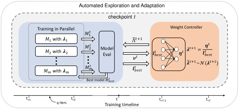
Figure 2: Illustration of the Automated Exploration and Adaptation in our Ada-Segment framework. It views the whole training process as a series of checkpoints ( $T$ checkpoints in total). The weight controller is trained interactively with $m$ models trained in parallel and evaluated at each checkpoint.

Overview

The common architectures (Kirillov et al. 2019; Xiong et al. 2019) tackle panoptic segmentation using a multi-objective model with several additional losses (e.g., losses from box head, segmentation head etc.). Given the loss vector $\boldsymbol{l}\in\mathbb{R}^{n}$ and their corresponding loss weight vector $\boldsymbol{\lambda}\in\mathbb{R}^{n}$ where $n$ is the number of training losses, we define the weighted loss of our panoptic segmentation framework as $L=\sum_{i=1}^{n}\lambda_{i}l_{i}$.

As stated previously, multi-loss weighting is essential but difficult in panotpic segmentation. Inspired by the adaptive learning and automated machine learning methods, the goal of our automated multi-loss adaptation (named Ada-Segment) framework is to automatically adjust $\boldsymbol{\lambda}$ during training via a controller. As Figure 2 shows, the controller is jointly trained with $m$ models (i.e., panotpic segmentation networks) $\{M_{1},M_{2},...,M_{m}\}$ training in parallel on a proxy training dataset (training set in short). After that, it can be used for controlling single model training at anytime.

Weight Controller

The weight controller is proposed to capture the training dynamics and automatically adjust loss weights during training. At the $t^{th}$ checkpoint, suppose the network produces the loss vector $\boldsymbol{l}^{t}$, and we want to find a weight vector $\boldsymbol{\lambda}^{t+1}$ to adjust the loss value so that the weighted loss can guide the network towards better optimization. Directly determine $\boldsymbol{\lambda}$ is impossible since we have no prior about it. However, since we know that the weighted loss vector is formulated as $\boldsymbol{\eta}^{t}=\boldsymbol{\lambda}^{t+1}\odot\boldsymbol{l}^{t}$ where $\odot$ is the element-wise multiplication. We introduce the weight controller to estimate the weighted loss vector as the transformation of the current loss vector as $\boldsymbol{\eta}^{t}=\pi(\boldsymbol{l}^{t};\theta),$ where $\theta$ is the learnable parameter in the weight controller $\pi$. Therefore, we can obtain the weight vector $\boldsymbol{\lambda}^{t+1}$ by

$$\boldsymbol{\lambda}^{t+1}=\frac{\boldsymbol{\eta}^{t}}{\boldsymbol{l}^{t}}=\frac{\pi(\boldsymbol{l}^{t};\theta)}{\boldsymbol{l}^{t}}.$$ (1)

Weight Controller Optimization. In this work, we use a policy network as the weight controller to predict the estimated weighted loss based on the loss at each time checkpoint. Since the loss weights directly determine the training loss, it may get into a dilemma if we use training loss to optimize the policy network through back-propagation. Some optimization technics are proposed by previous works (Kendall et al. 2018; Chen et al. 2017), however, they are still unstable and even lead to divergence when directly using training gradients to optimize weights on complex tasks like panoptic segmentation. Therefore, we optimize the policy network towards the evaluation metric (i.e., PQ in panoptic segmentation) via the validation set through REINFORCE (Williams 1992).

State Space: During training, at any time checkpoint $t$, the policy network takes the loss vector $\boldsymbol{l}^{t}$ to represent the optimization state of the model, and outputs the estimated weighted loss $\boldsymbol{\eta}^{t}$ to calculate $\boldsymbol{\lambda^{t+1}}$.

Action Space: Exploration is of great importance to find improved solution via an action space design. We sample loss weight candidates $\hat{\Lambda}^{t+1}=\{\boldsymbol{\hat{\lambda}}^{t+1}_{1},\boldsymbol{\hat{\lambda}}^{t+1}_{2},...,\boldsymbol{\hat{\lambda}}^{t+1}_{m}\}$ to train $m$ models from a Normal distribution

$$\boldsymbol{\hat{\lambda}}^{t+1}\sim\mathcal{N}(\boldsymbol{\lambda^{t+1}},\sigma),$$ (2)

in which $\boldsymbol{\lambda^{t+1}}$ is uesd as the mean value and $\sigma$ is the sampling standard deviation.

Rewards: Reward function $r(\cdot)$ measures the quality of the generated actions. Intuitively, after applying the actions, we can use the models’ performances (PQ) as the policy rewards to guide the training of the policy network. We refer this as the local reward function

$$r_{local}(\boldsymbol{v}^{t})=\frac{\boldsymbol{v}^{t}-mean(\boldsymbol{v}^{t})}{std(\boldsymbol{v}^{t})},$$ (3)

which normalizes the validation performances $\boldsymbol{v}^{t}\in\mathbb{R}^{m}$ at checkpoint $t$ to zero mean and unit variance as rewards.

Furthermore, we include the relative improvement from the previous checkpoint as the policy rewards:

$$r_{imp}(\boldsymbol{v}^{t}_{imp})=\frac{\boldsymbol{v}^{t}_{imp}}{std(\boldsymbol{v}^{t}_{imp})},$$ (4)

which calculates the normalized absolute improvement from the previous checkpoint to introduce long-range influences where $\boldsymbol{v}^{t}_{imp}=\boldsymbol{v}^{t}-v^{t-1}_{best}.$ This is non-trivial because only using the differences between temporal samples would overlook the training dynamics between checkpoints.

Therefore, the overall rewards are calculated as

$$r(\boldsymbol{v}^{t})=\frac{t}{T}(r_{local}(\boldsymbol{v}^{t})+r_{imp}(\boldsymbol{v}^{t}_{imp})),$$ (5)

where the scale factor $\frac{t}{T}$ controls the magnitude of the overall reward according to the training process since the early training stages are less important with more randomness.

Parameter Updates: Given the sample rewards, the parameter $\theta$ of the policy network $\pi$ is updated by the gradients

$$\nabla_{\theta}R^{t}(\theta)=\frac{1}{m}\sum_{j=1}^{m}{r^{t}_{j}(\boldsymbol{v}^{t})\nabla_{\theta}\log{s(\boldsymbol{\hat{\lambda}}^{t+1}_{j};\frac{\pi(\boldsymbol{l}^{t};\theta)}{\boldsymbol{l}^{t}},\sigma)}},$$ (6)

where $s(\cdot;\mu,\sigma)$ is the probability density function of the Normal distribution. It is worth noting that we only consider the situation that all loss values are nonnegative, which is the common scenario in panoptic segmentation. Therefore, when sampling from the Normal distribution, samples contain negative values would be given $-1$ as the reward directly to increase the training stability.

Ada-Segment Algorithm

In this section, we introduce how the overall Ada-Segment framework works in detail.

Initial State. Since the policy network requires training losses as input. At the very beginning, one pseudo training epoch is performed with all loss weights equal to 1 before the exact training schedule to obtain the initial loss $\boldsymbol{l}^{1}$.

Policy Initilaization The initial policy is crucial for training stability. All layers in the policy network are randomly initialized by the Normal distribution with mean value equal to $1/n_{c}$ instead of $0$ to avoid the loss weights to be non-positive at the beginning (except the bias parameters is initialized to 0), where $n_{c}$ is the number of input channels of each layer.

Automated Exploration and Adaptation. In this phase, the controller and $m$ models are jointly trained as shown in Figure 2. Between two checkpoints, we train models in parallel with separate loss weights generated by the weight controller and track the training losses. At each checkpoint, we evaluate all models on the validation set, obtaining the model performances $\boldsymbol{v}^{t}$ (i.e., PQ value on validation for panoptic segmentation) to calculate rewards following Equatin 5. The policy network is updated by gradients descent via Equation 6. To continue training, we broadcast the best-performed model to all other models, thus we can use $l^{t}_{best}$ as the training condition at each time checkpoint.

Policy Transfer. We can get the best-performed model $M^{T}_{best}$ after the exploration phase. However, we take it a step further and propose the policy transfer. Our framework, once finished one exploration process, also produces the trained controller that gives us the chance to re-use it at anytime, saving the time and computational cost when the dataset or training schedule changes.

Along with the training of the model, the policy network is changing accordingly, causing the policy $\pi^{T}$ may favor the latest training condition but partly forget former loss situations. Besides, earlier states of policy may suffer from the under-fitting problem with few update iterations. Therefore, to make full use of the controller, we proposed to combine all states of the policy network during exploration phase i.e., $\pi^{1}$ to $\pi^{T}$, via a weighted policy ensemble strategy.

When training a model $M_{p}$ for $E$ epochs and adjusting loss weights every training epoch, with $E$ is not necessary to be equal to $T$. By calculating the distance between a training epoch $e$ and corresponding update checkpoint $t$, we can assign a weight to each policy state at different training epochs controlled by a discount factor $\gamma=0.9$. Therefore, we have

$$\boldsymbol{\lambda}^{e+1}=\frac{1}{Z}\sum^{T}_{t}{\gamma^{\lvert\frac{e\times T}{E}-t\rvert}\frac{\pi^{t}(\boldsymbol{l}^{e};\theta)}{\boldsymbol{l}^{e}}},$$ (7)

where $\frac{T}{E}$ align the training procedure with the number of exploration checkpoints and $Z=\sum^{T}_{t}{\gamma^{\lvert\frac{e\times T}{E}-t\rvert}}$ is the normalizing factor. By combining policy states at different stages, the training dynamics captured by the policy network can be preserved to a large extend. To sum up, the paradigm of our Ada-Segment is summarized in Algorithm 1.

Input: Iterations between two checkpoints $q$, Initial Loss State $\boldsymbol{l}^{1}$, Number of checkpoints $T$, Number of training epochs $E$

Initialize $m$ models $\{M_{1},M_{2},...M_{m}\}$

Initialize policy network $\pi$

$\boldsymbol{l}_{best}^{1}\leftarrow\boldsymbol{l}^{1}$

for $t\leftarrow 1$ to $T$, do

Generate $\boldsymbol{\lambda}^{t+1}$ by Equation 1 with $\pi$ and $\boldsymbol{l}_{best}^{t}$

Sample $m$ candidates by Equation 2 with $\boldsymbol{\lambda}^{t+1}$

Train all models for $q$ iterations with $\hat{\Lambda}^{t+1}$

Collect model performances $\boldsymbol{v}^{t}$ and save $\boldsymbol{l}_{best}^{t}$

Obtain policy rewards by Equation 5

Update $\theta$ in $\pi$ via Equation 6

Save $\pi^{t}\leftarrow\pi$

Update all models with $M_{best}^{t}$

end for

Initialize a model $M_{p}$

for $e\leftarrow 1$ to $E$, do

Generate $\boldsymbol{\lambda}^{e+1}$ by Equation 7 with $\boldsymbol{l}^{e}$

Train model $M_{p}$ with $\boldsymbol{\lambda}^{e+1}$

end for

return $M^{p}$

Algorithm 1 The Ada-Segment framework.

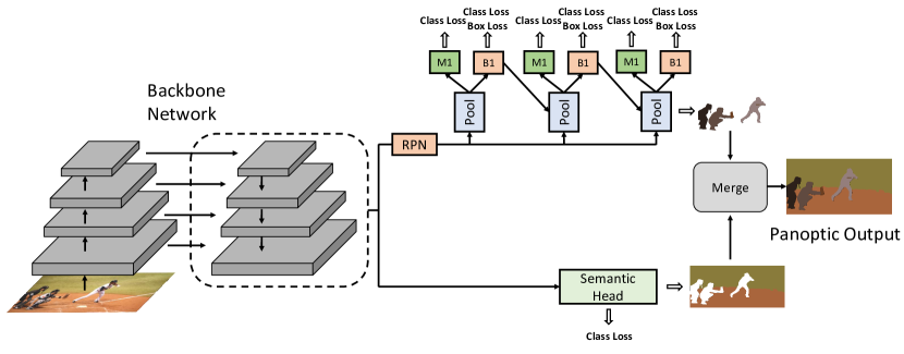
Figure 3: The network structure of our baseline. For detection branch, we use the three-stage Cascade R-CNN (Cai and Vasconcelos 2018), which contains three pairs of losses. The semantic segmentation branch is a simple SemanticFPN in (Kirillov et al. 2019). The overall architecture has ten losses to be jointly optimized.

Network Structure

Figure 3 shows the network structure used in our experiments, which extends Cascade Mask R-CNN (Cai and Vasconcelos 2018) with a semantic segmentation branch.

Backbone Networks. We use a ResNet (He et al. 2015a) with a Feature Pyramid Network (FPN) (Lin et al. 2017). and add deformable convolution (Dai et al. 2017) in stage $3\sim 5$ of the backbone networks.

Instance Segmentation Head. We use three cascaded detection heads after region proposal network in our network. To get the instance segmentation results, each stage of head outputs bounding box regression, classification and mask results for objects in an image.

Semantic Segmentation Head. We use a semantic segmentation head following Panotic FPN (Kirillov et al. 2019). It takes the FPN features as inputs and uses 1x1 convolution and bi-linear upsample function to gradually upsample each FPN feature to 1/4 of input image size. All upsampled features are summed up and transformed into the final segmentation map by a 1x1 convolution.

Experiments

Datasets and Evaluation

COCO. Following the competition setting in 2019 Microsoft COCO panoptic segmentation, which consists of 133 classes with 80 things classes and 53 stuff classes. We only use train2017 split with approximately 118k images for training and report the results on val split with 5k images. We also report our results on COCO test-dev split for comparison with other state-of-the-art methods.

ADE20K. ADE20K is a challenging dataset with densely labeled 22k images, with 100 things classes and 50 stuff classes. It contains heavier occlusions, more tiny objects and class ambiguities than COCO, and thus more challenging.

Proxy Dataset Setting. In the practice of automated machine learning, for evaluation during training, it is necessary to construct a proxy validation dataset instead of using the original validation set. For COCO, we randomly sample 10k images from the 118k training set for validation and the rest part as the proxy training set. For ADE20K, we train on 20k training images in which 2k images are randomly sampled images for validation during training.

Evaluation Setup. We follow the panoptic segmentation evaluation metrics proposed in (Kirillov et al. 2018) to evaluate our models in terms of panoptic quality (PQ), segmentation quality (SQ) and recognition quality (RQ). Note that PQ is the weighted sum of PQ^th and PQ^st for things and stuff classes respectively. We report these two metrics for demonstrating the effectiveness of our method.

Method	training set	PQ	PQth	PQst
Baseline	COCOp	40.7	47.1	31.0
Baseline-G	COCOp	41.7+1.0	48.7+1.6	31.1+0.1
Baseline-P	COCOp	41.1+0.4	48.8+1.7	29.4-1.6
Ada-Segment-A	COCOp	42.6+1.9	49.5+2.4	32.1+1.1
Ada-Segment	COCOp	43.2+2.5	50.5+3.4	32.3+1.3
Baseline	COCO	41.0	47.2	31.5
Baseline-G	COCO	42.1+1.1	49.0+1.8	31.6+0.1
Ada-Segment	COCO	43.7+2.7	51.2+4.0	32.5+1.0

Table 1: Comparison with different baselines on COCO val split. All models are trained on the proxy training set. Baseline-G: using coarse grid search to optimize loss weights with multiple runs. Baseline-P: applying a PBT-like (Jaderberg et al. 2017) framework to tune loss weights during training, which can be viewed as our method without the weight controller. $COCO_{p}$ represents the proxy dataset.

Method	Weighting Type	PQ	PQth	PQst
Baseline	static	41.0	47.2	31.5
Baseline-G	static	42.1	49.0	31.6
Final	static	42.2	50.0	30.4
Pred	static	42.6	50.3	31.0
Single-dy	dynamic	43.1	50.1	32.4
Comb-dy	dynamic	43.7	51.2	32.5

Table 2: Comparison of different static weighting strategy and different dynamical adaptation strategy on COCO.

Train Arch.	Trans. Arch	Train Data	Trans. Data	Train. Sche.	Tran. Sche.	PQ	PQth	PQst
R-50	R-50	ADE20Kp	COCO	1x	1x	42.7	49.0	33.1
R-50	R-50	COCOp	COCO	1x	1x	43.7	51.2	32.5
R-50	R-50	COCOp	ADE20K	1x	1x	32.0	34.3	27.4
R-50	R-50	ADE20Kp	ADE20K	1x	1x	32.9	35.6	27.9
R-50	R-101	COCOp	COCO	1x	1x	45.1	52.7	33.6
R-101	R-101	COCOp	COCO	1x	1x	45.2	52.2	34.7
R-50	R-50	COCOp	COCO	1x	2x	44.3	51.3	33.7
R-50	R-50	COCOp	COCO	2x	2x	44.4	50.9	34.5

Table 3: Transferability of the policy network across different backbones, training schedules and datasets. $D_{p}$ means searching and training on the proxy dataset. 1x: 12 epochs on COCO or 24 epochs on ADE20K; 2x: training for 24 epochs on COCO.

Method	PQ	PQth	PQst
Panoptic FPN†	38.1	43.8	29.4
Panoptic FPN‡	39.0+0.9	46.1+2.3	28.3-1.1
Panoptic FPN⋆	39.0+0.9	45.9+2.1	28.7-0.7
w Ada-Segment	39.9+1.8	46.6+2.8	29.7+0.3

Table 4: Multi-loss adaptation for Panoptic FPN (Kirillov et al. 2019) on COCO, ${\dagger}$: our re-implementation with all loss weights equal to 1; $\ddagger$: our re-implementation with loss weights used in the paper; $\star$: results reported in the paper.

Implementation Details

Model Training. We follow the commonly used hyper-parameter settings as stated in Panoptic FPN (Kirillov et al. 2019) within our experiments. We set the initial learning rate as 0.02 and weight decay as 0.0001 with stochastic gradient descent (SGD) for all experiments. To provide more stable information to train the policy network, we decrease learning rate with cosine policy, which is more smooth than decrease the learning rate at specific iterations. We initialize the backbone network with ImageNet pretrained model while the remaining parameters are initialized following (He et al. 2015b). For each model, we train totally 12 epochs (so called 1x setting) for COCO and 24 epochs for ADE20K on 8 GPUs with 2 images per GPU using PyTorch (Paszke et al. 2017).

Automated Multi-loss Adaptation. During joint training, we deploy $m=8$ models, where each model contains $n=10$ losses: three pairs of instance detection losses (bounding box loss, classification loss and mask loss) and a single semantic segmentation loss. In the weight controller, we set the sampling standard deviation $\sigma=0.2$, and we use three-layer MLP with hidden layer size 16 as the policy network. We use Adam (Kingma and Ba 2014) optimizer with learning rate $5e^{-2}$ and weight decay $5e^{-4}$ to optimize the policy network. For the overall Ada-Segement framework, we simply train 1 Epoch between two checkpoints for both COCO and ADE20K datasets. When adjusting loss weight, we re-scale the learning rate of the $i^{th}$ head by $\frac{1}{\lambda_{i}}$ for $i=1,2,...,n$ to ensure the head networks to be fully trained so that the loss weights only influence the shared backbone and the detection losses are averaged among three cascade stages.

Inference. The panoptic results are obtained in the way proposed in (Kirillov et al. 2018). Specifically, after merging instance masks on the non-overlap canvas, the remaining pixels are assigned according to semantic segmentation results (with areas less than 4096 being ignored).

Baseline Setup. The baseline method means setting equaling weights (with value 1) during training. As to be shown in the following sections, although a strong baseline network is used, it only produces unsatisfactory results, which is inhibited by the improper weight setting. Without particular notions, we report results with ResNet-50 backbone.

Methods	backbone	PQ	PQth	PQst	SQ	RQ
Panoptic FPN (Kirillov et al. 2019)	ResNet-101-FPN	40.9	48.3	29.7	-	-
OANet (Liu et al. 2019)	ResNet-101-FPN	41.3	50.4	27.7	-	-
AUNet (Li et al. 2019b)	ResNeXt-152-FPN-D	46.5	55.8	32.5	81.0	56.1
UPSNet (Xiong et al. 2019)	ResNet-101-FPN-D	46.6	53.2	36.7	80.5	56.9
OCFusion (Lazarow et al. 2020)	ResNeXt-101-FPN-D	46.7	54.0	35.7	-	-
SpatialFlow (Chen et al. 2019)	ResNet-101-FPN-D	47.3	53.5	37.9	81.8	56.9
BANet (Chen et al. 2020)	ResNet-101-FPN-D	47.3	54.9	35.9	80.8	57.5
SOGNet(Yang et al. 2019)	ResNet-101-FPN-D	47.8	-	-	80.7	57.6
Ours	ResNet-101-FPN-D	48.5	55.7	37.6	81.8	58.2

Table 5: Results on COCO test-dev split. In the table, ’-D’ represents methods using deformable convolution (Zhu et al. 2019) in the backbone networks. We achieve the best things-stuff trade-off to get best final PQ results.

Method	PQ	PQth	PQst	Type	Cost
Baseline	41.0	47.2	31.5	-	1x
GradNorm	41.8	48.0	32.4	G	$\sim$2x
Grid Search	42.1	49.0	31.6	S	$\sim$20x
PBT	41.4	49.1	29.8	S	$\sim$8x
AM-LFS	41.7	50.1	28.9	R	$\sim$8x
BOHB	42.0	50.0	29.9	B	$\sim$8x
Ada-Segment	43.7±0.1	51.2±0.07	32.5±0.14	R	$\sim$8x+1x

Table 6: Comparison with different types of automated tuning methods on COCO val split, including GradNorm (Chen et al. 2017), Grid Search, PBT (Jaderberg et al. 2017), AM-LFS (Li et al. 2019a) and BOHB (Falkner et al. 2018), on COCO val set based on our baseline network (R-50 backbone). G: Gradient-Based, S: Sample-Based B: BO-Based, R: RL-guided. We ran Ada-Segment 3 times with different random seeds and report in format of mean$\pm$std.

Ablation Studies

Main Results. We compare with different baselines in Table 1. Compared with the vanilla baseline using all weights equal to 1, our method achieves 43.7% PQ, bringing 2.7% performance gain. One may argue that whether the vanilla baseline is appropriate since we introduce more computational cost and the vanilla weight setting may have bias on different network structures. Therefore, we provide an alternate baseline named baseline-G following the way used in (Kirillov et al. 2019), which treats detection losses as a single group and performs grid search on detection and segmentation loss weights. It can be seen that our Ada-Segment also achieves 1.5% performance gains.

Effectiveness of Weight Controller. To validate the effectiveness of the weight controller, in the top part of Table 1, we remove the weight controller to see whether it could work well when only synchronize all models at each time checkpoints with different loss weights generated by an evolution strategy. This setting resembles Population Based Training (Jaderberg et al. 2017), and is also used as a baseline named by baseline-P. The results suggest that the controller contributes most in the loss weights adaption.

Besides, we can obtain the best-performed model $M^{T}_{best}$ after Automated Exploration and Adaptation phase. We also report the performance of $M^{T}_{best}$ as Ada-Segment-A in table 1, which can already brings 1.9% PQ gain compared with the vanilla baseline and outperforms baseline-G by 0.9%. When train model with the controller using policy ensemble, additional 0.6% performance gain is obtained, demonstrating that the controller did learn the potential training pattern and benefit the model training.

Superiority of Training Dynamics. Different from the a static weighting strategy, we leverage the weight controller to dynamically adjust training loss weights. One may have the question that whether it is enough to use the policy network to give a static weight setting that benefits the whole training process. We validate this concern by trying the following settings: 1) Final: training with the final loss weights $\boldsymbol{\lambda}_{best}^{T}$ of the Exploration and Adaptation phase. 2) Pred: using the final policy network to predict a static loss weights (based on the initial loss) to train the model. 3) Single-dy: using the final policy network to guide the training process. 4) Comb-dy: using the weight controller with the policy ensemble strategy during the training process.

The results in Table 2 demonstrate the significant advantage of dynamically adapting the loss weights during training. Using policy ensemble to combine all states of policy networks improves the final state of policy network $\pi^{T}$ by 0.6%. This is not surprising since the policy network is continuous updating in the exploration phase, and the final state may not well suite for the begining stages. It also suggests that there do exists ever-chaning convergence dynamics during panoptic model training.

Generalization Capability across Network Structures. The main results of our method are carried our on a well-developed network to show the problem that loss weighting inhibits the network-level design. One may curios about whether our framework can also work well on a simple network with less losses. To validate the generalization capability of our framework, we apply our Ada-Segment strategy to the simple Panoptic FPN (Kirillov et al. 2019), which uses Mask R-CNN (He et al. 2017) as base detector with three detection losses (bounding box regression / classification, mask segmentation losses) and uses the same segmentation head as used in our network, and the results are shown in Table 4.

It can be seen that although the network contains fewer losses than the network used in our method (4 vs 10 losses), the imbalance problem is also serious since it degrades 0.9% PQ and 2.3% PQ^th. With our Ada-Segment, we boost the performance of both PQ^th and PQ^st and improve the final performance by 1.8% PQ from the vanilla weighting and 0.9% from the well-tuned baseline.

Policy Transferability. In Table 3, we evaluate the transferability of the policy network on different backbones, training schedules and datasets. It can be found that, 1) the policy benefits model training when transfer from ADE20K to COCO. 2) Policy from COCO also has a positive effect on ADE20K (32.0% vs. 31.6% baseline) and comparable with grid-search baseline (32.1%). 3) Policy trained along with small backbone network also works well on larger backbone. 4) Policy obtained from short training schedule can also be apply on longger training schedule, suggesting that the training dynamics of different training schedules are similar.

Reward Function Design. When only using $r_{local}$ as rewards, the controller learns from the relative differences between sampled actions but overlooks the training dynamics between checkpoints, which only get 42.6% PQ finnally. With $r_{imp}$, the controller is trained much well to get 43.7% PQ.

Comparison with other methods

Panoptic Segmentation on COCO. We compare our proposed network with other state-of-the-art methods on COCO test-dev split in Table 5. With the proposed method, we achieve the PQ performance 48.5%, which is the state-of-the-art results produced by a single model without extra training data. It is worth noting that although our method does not report top performance on neither PQ^th nor PQ^st on test-dev set, we achieve the best things-stuff trade-off to get best final PQ results with our Ada-Segment to reconcile multiple subtask losses during training while previous works may favor one of the metrics and degrade another.

Automated Tuning Methods. Our method can be seen as an online hyperparameter tuning framework. In Table 6, we compare our Ada-Segment with different types of automated tuning methods to show the practicability and effectiveness of our method. Grid search and PBT(Jaderberg et al. 2017) are used as special baselines of as showed in the previous sections. GradNorm (Chen et al. 2017) is an effective multi-objective learning method that adjusts subtask gradients during back-propagation. We implement AM-LFS(Li et al. 2019a) to directly optimize the loss weights, which performs poorly on $PQ^{st}$, which suggests that our weight controller perfors much better than the greedy optimization.

Besides, when treating the loss weights as hyperparameters, we compare with BOHB (Falkner et al. 2018), the state-of-the-art hyperparameter optimization method, which performs much worse than our automated adaptation strategy since it only searches for a static parameter setting, missing the chance to adjust losses at different training stages.

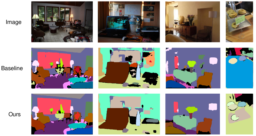
Figure 4: Qualitative comparison of the results produced by our baseline and the results using Ada-Segment for training.

Qualitative Results

In Figure 4, the results produced by our method are visually precise and coherent for both foreground objects and background stuff and the results output by our baseline contain some fuzzy part due to inappropriate training. More qualitative results can be found in the Appendix.

Conclusion

In this work, we propose a novel automated online multi-loss adaptation framework named Ada-Segment for panoptic segmentation. We emphasize the importance of dynamically adjusting the loss weights and propose the online multi-loss adaptation strategy with an effective and efficient weight controller, which achieves state-of-the-art performances on COCO and ADE20K panoptic segmentation benchmarks. We hope our work will give researchers in this area new insights to focus on the training level design.

Acknowledgments. This work was supported in part by National Natural Science Foundation of China (NSFC) under Grant No.U19A2073 and No.61976233, Guangdong Province Basic and Applied Basic Research (Regional Joint Fund-Key) Grant No.2019B1515120039, Nature Science Foundation of Shenzhen Under Grant No. 2019191361, Zhijiang Lab’s Open Fund (No. 2020AA3AB14) and CSIG Young Fellow Support Fund.

References

- Baydin et al. (2017) Baydin, A. G.; Cornish, R.; Rubio, D. M.; Schmidt, M.; and Wood, F. 2017. Online learning rate adaptation with hypergradient descent. arXiv preprint arXiv:1703.04782 .
- Bengio et al. (2009) Bengio, Y.; Louradour, J.; Collobert, R.; and Weston, J. 2009. Curriculum learning. In Proceedings of the 26th annual international conference on machine learning, 41–48. ACM.
- Cai and Vasconcelos (2018) Cai, Z.; and Vasconcelos, N. 2018. Cascade R-CNN: Delving into High Quality Object Detection. In CVPR.
- Chen et al. (2019) Chen, Q.; Cheng, A.; He, X.; Wang, P.; and Cheng, J. 2019. SpatialFlow: Bridging All Tasks for Panoptic Segmentation. arXiv preprint arXiv:1910.08787 .
- Chen et al. (2020) Chen, Y.; Lin, G.; Li, S.; Bourahla, O.; Wu, Y.; Wang, F.; Feng, J.; Xu, M.; and Li, X. 2020. BANet: Bidirectional Aggregation Network with Occlusion Handling for Panoptic Segmentation. In Proceedings of the IEEE/CVF Conference on Computer Vision and Pattern Recognition, 3793–3802.
- Chen et al. (2017) Chen, Z.; Badrinarayanan, V.; Lee, C.-Y.; and Rabinovich, A. 2017. Gradnorm: Gradient normalization for adaptive loss balancing in deep multitask networks. arXiv preprint arXiv:1711.02257 .
- Cheng et al. (2019) Cheng, B.; Collins, M. D.; Zhu, Y.; Liu, T.; Huang, T. S.; Adam, H.; and Chen, L.-C. 2019. Panoptic-DeepLab: A Simple, Strong, and Fast Baseline for Bottom-Up Panoptic Segmentation. arXiv preprint arXiv:1911.10194 .
- Dai et al. (2017) Dai, J.; Qi, H.; Xiong, Y.; Li, Y.; Zhang, G.; Hu, H.; and Wei, Y. 2017. Deformable convolutional networks. In Proceedings of the IEEE international conference on computer vision, 764–773.
- Falkner et al. (2018) Falkner, S.; Klein, A.; Hutter, F.; and et al. 2018. BOHB: Robust and efficient hyperparameter optimization at scale. arXiv preprint arXiv:1807.01774 .
- Farhadi et al. (2009) Farhadi, A.; Endres, I.; Hoiem, D.; and Forsyth, D. 2009. Describing objects by their attributes. In CVPR.
- Feurer and Hutter (2019) Feurer, M.; and Hutter, F. 2019. Hyperparameter optimization. In Automated Machine Learning, 3–33. Springer, Cham.
- He et al. (2017) He, K.; Gkioxari, G.; Dollár, P.; and Girshick, R. 2017. Mask r-cnn. In ICCV, 2961–2969.
- He et al. (2015a) He, K.; Zhang, X.; Ren, S.; and Sun, J. 2015a. Deep Residual Learning for Image Recognition. arXiv preprint arXiv:1512.03385 .
- He et al. (2015b) He, K.; Zhang, X.; Ren, S.; and Sun, J. 2015b. Delving deep into rectifiers: Surpassing human-level performance on imagenet classification. In Proceedings of the IEEE international conference on computer vision, 1026–1034.
- Huang et al. (2019) Huang, C.; Zhai, S.; Talbott, W.; Bautista, M. A.; Sun, S.-Y.; Guestrin, C.; and Susskind, J. 2019. Addressing the Loss-Metric Mismatch with Adaptive Loss Alignment. arXiv preprint arXiv:1905.05895 .
- Hutter et al. (2011) Hutter, F.; Hoos, H. H.; Leyton-Brown, K.; and et al. 2011. Sequential model-based optimization for general algorithm configuration. In International conference on learning and intelligent optimization, 507–523. Springer.
- Jaderberg et al. (2017) Jaderberg, M.; Dalibard, V.; Osindero, S.; Czarnecki, W. M.; Donahue, J.; Razavi, A.; Vinyals, O.; Green, T.; Dunning, I.; Simonyan, K.; et al. 2017. Population based training of neural networks. arXiv preprint arXiv:1711.09846 .
- Kendall et al. (2018) Kendall, A.; Gal, Y.; Cipolla, R.; and et al. 2018. Multi-task learning using uncertainty to weigh losses for scene geometry and semantics. In Proceedings of the IEEE Conference on Computer Vision and Pattern Recognition, 7482–7491.
- Kingma and Ba (2014) Kingma, D. P.; and Ba, J. 2014. Adam: A method for stochastic optimization. arXiv preprint arXiv:1412.6980 .
- Kirillov et al. (2019) Kirillov, A.; Girshick, R.; He, K.; and Dollár, P. 2019. Panoptic Feature Pyramid Networks. arXiv preprint arXiv:1901.02446 .
- Kirillov et al. (2018) Kirillov, A.; He, K.; Girshick, R.; Rother, C.; and Dollár, P. 2018. Panoptic segmentation. arXiv preprint arXiv:1801.00868 .
- Kokkinos (2017) Kokkinos, I. 2017. Ubernet: Training a universal convolutional neural network for low-, mid-, and high-level vision using diverse datasets and limited memory. In Proceedings of the IEEE Conference on Computer Vision and Pattern Recognition, 6129–6138.
- Lazarow et al. (2020) Lazarow, J.; Lee, K.; Shi, K.; and Tu, Z. 2020. Learning instance occlusion for panoptic segmentation. In Proceedings of the IEEE/CVF Conference on Computer Vision and Pattern Recognition, 10720–10729.
- Li et al. (2019a) Li, C.; Yuan, X.; Lin, C.; Guo, M.; Wu, W.; Yan, J.; and Ouyang, W. 2019a. Am-lfs: Automl for loss function search. In Proceedings of the IEEE International Conference on Computer Vision, 8410–8419.
- Li et al. (2017) Li, L.; Jamieson, K.; DeSalvo, G.; Rostamizadeh, A.; and Talwalkar, A. 2017. Hyperband: A novel bandit-based approach to hyperparameter optimization. The Journal of Machine Learning Research 18(1): 6765–6816.
- Li et al. (2019b) Li, Y.; Chen, X.; Zhu, Z.; Xie, L.; Huang, G.; Du, D.; and Wang, X. 2019b. Attention-guided unified network for panoptic segmentation. In CVPR.
- Lin et al. (2017) Lin, T.-Y.; Dollár, P.; Girshick, R.; He, K.; Hariharan, B.; and Belongie, S. 2017. Feature pyramid networks for object detection. In CVPR, 2117–2125.
- Lin et al. (2018) Lin, T.-Y.; Goyal, P.; Girshick, R.; He, K.; and Dollár, P. 2018. Focal loss for dense object detection. IEEE transactions on pattern analysis and machine intelligence .
- Liu et al. (2019) Liu, H.; Peng, C.; Yu, C.; Wang, J.; Liu, X.; Yu, G.; and Jiang, W. 2019. An End-to-End Network for Panoptic Segmentation. In CVPR.
- Paszke et al. (2017) Paszke, A.; Gross, S.; Chintala, S.; Chanan, G.; Yang, E.; DeVito, Z.; Lin, Z.; Desmaison, A.; Antiga, L.; and Lerer, A. 2017. Automatic differentiation in PyTorch. In NIPS Workshop.
- Pedregosa (2016) Pedregosa, F. 2016. Hyperparameter optimization with approximate gradient. arXiv preprint arXiv:1602.02355 .
- Porzi et al. (2019) Porzi, L.; Bulo, S. R.; Colovic, A.; and Kontschieder, P. 2019. Seamless scene segmentation. In Proceedings of the IEEE Conference on Computer Vision and Pattern Recognition, 8277–8286.
- Ren et al. (2018) Ren, M.; Zeng, W.; Yang, B.; and Urtasun, R. 2018. Learning to reweight examples for robust deep learning. arXiv preprint arXiv:1803.09050 .
- Snoek et al. (2012) Snoek, J.; Larochelle, H.; Adams, R. P.; and et al. 2012. Practical bayesian optimization of machine learning algorithms. In Advances in neural information processing systems, 2951–2959.
- Tu et al. (2005) Tu, Z.; Chen, X.; Yuille, A. L.; and Zhu, S.-C. 2005. Image parsing: Unifying segmentation, detection, and recognition. International Journal of computer vision 63(2): 113–140.
- Williams (1992) Williams, R. J. 1992. Simple statistical gradient-following algorithms for connectionist reinforcement learning. Machine learning 8(3-4): 229–256.
- Wu et al. (2020a) Wu, Y.; Zhang, G.; Gao, Y.; Deng, X.; Gong, K.; Liang, X.; and Lin, L. 2020a. Bidirectional Graph Reasoning Network for Panoptic Segmentation. In Proceedings of the IEEE/CVF Conference on Computer Vision and Pattern Recognition, 9080–9089.
- Wu et al. (2020b) Wu, Y.; Zhang, G.; Xu, H.; Liang, X.; and Lin, L. 2020b. Auto-Panoptic: Cooperative Multi-Component Architecture Search for Panoptic Segmentation. Advances in Neural Information Processing Systems 33.
- Xiong et al. (2019) Xiong, Y.; Liao, R.; Zhao, H.; Hu, R.; Bai, M.; Yumer, E.; and Urtasun, R. 2019. UPSNet: A Unified Panoptic Segmentation Network. arXiv preprint arXiv:1901.03784 .
- Xu et al. (2018) Xu, H.; Zhang, H.; Hu, Z.; Liang, X.; Salakhutdinov, R.; and Xing, E. 2018. AutoLoss: Learning Discrete Schedules for Alternate Optimization. arXiv preprint arXiv:1810.02442 .
- Yang et al. (2019) Yang, Y.; Li, H.; Li, X.; Zhao, Q.; Wu, J.; and Lin, Z. 2019. SOGNet: Scene Overlap Graph Network for Panoptic Segmentation. arXiv preprint arXiv:1911.07527 .
- Zeiler (2012) Zeiler, M. D. 2012. Adadelta: an adaptive learning rate method. arXiv preprint arXiv:1212.5701 .
- Zhu et al. (2019) Zhu, X.; Hu, H.; Lin, S.; and Dai, J. 2019. Deformable convnets v2: More deformable, better results. In Proceedings of the IEEE Conference on Computer Vision and Pattern Recognition, 9308–9316.