DIPPAS: A Deep Image Prior PRNU Anonymization Scheme

Abstract

Source device identification is an important topic in image forensics since it allows to trace back the origin of an image. Its forensics counter-part is source device anonymization, that is, to mask any trace on the image that can be useful for identifying the source device. A typical trace exploited for source device identification is the Photo Response Non-Uniformity (PRNU), a noise pattern left by the device on the acquired images. In this paper, we devise a methodology for suppressing such a trace from natural images without significant impact on image quality. Specifically, we turn PRNU anonymization into the combination of a global optimization problem in a Deep Image Prior (DIP) framework followed by local post-processing operations. In a nutshell, a Convolutional Neural Network (CNN) acts as generator and iteratively returns several images with attenuated PRNU traces. By exploiting a straightforward local post-processing and assembly on these images, we produce a final image that is anonymized with respect to the source PRNU, still maintaining high visual quality. With respect to widely-adopted deep learning paradigms, the used CNN is not trained on a set of input-target pairs of images. Instead, it is optimized to reconstruct output images from the original image under analysis itself. This makes the approach particularly suitable in scenarios where large heterogeneous databases are analyzed and prevents any problem due to lack of generalization. Through numerical examples on publicly available datasets, we prove our methodology to be effective compared to state-of-the-art techniques.

Research

1 Introduction

Source device identification is a well-studied problem in the multimedia forensics community [1, 2, 3, 4]. Indeed, identifying the source camera of an image helps to trace its origin and verifying its integrity. Many state-of-the-art techniques tackle this problem by relying on Photo Response Non-Uniformity (PRNU), which is a unique characteristic noise pattern left by the device on each acquired content [1]. Given a query image and a candidate device, it is possible to infer whether the image was shot by the device with a cross-correlation test between a noise trace extracted from the image and the device PRNU [5].

Despite the effort put into developing robust PRNU-based source attribution techniques, the forensic community has also focused on studying the possibility of removing PRNU traces from images. On one hand, determining at which level PRNU can be actually removed is essential to study the robustness of PRNU-based forensic detectors, and possibly improve them. On the other hand, when privacy is a concern, being able to link a picture to its owner is clearly undesirable. As an example, photojournalists carrying out legit investigations may prefer to anonymize their shots to avoid being threatened.

For these reasons, counter-forensic methods that enable deleting or reducing PRNU traces from images have been proposed in the literature. We can broadly split the developed techniques into two families. The first family requires the knowledge of the PRNU pattern to be deleted, and we refer to them as PRNU-aware methods. This is the case of [6, 7, 8], which propose different iterative solutions to delete a known PRNU from a given picture. Specifically, [6] proposes an adaptive PRNU-based image denoising, removing an estimate of the PRNU from each image. Authors of [7] estimate the best subtraction weight that minimizes the cross-correlation between the PRNU and the trace extracted from the image to be anonymized. Recently, [8] applies a Convolutional Neural Network (CNN), which exploits the source PRNU to hinder its traces from a query image. The network is used as a parametric operator, which iteratively overfits the given pair of image and PRNU, imposing a minimization of their correlation.

The second family of methods works by blindly modifying pixel values in order to make the underlying PRNU unrecognizable. For instance, [9] shows that multiple image denoising steps can help attenuating the PRNU, even though this may not be enough to completely hinder its traces from images [10]. Alternatively, [11] applies seam-carving to change pixel locations, and [12] exploits patch-match techniques to scramble pixel positions. More recently, [13] proposes an inpainting-based method which deletes and reconstructs image pixels such that final images are anonymized with respect to their source PRNU.

In this manuscript, we propose an image anonymization tool leveraging a combination of a global optimization strategy (i.e., operating on the full image) and local post-processing operations. In particular, global optimization on the entire image is performed exploiting a CNN. Given an image to be anonymized and a reference PRNU trace to be removed, the proposed network iteratively generates multiple images where PRNU traces are attenuated, still maintaining high visual quality. Differently from most CNN works, the proposed network does not need a training step. In fact, the used CNN exploits the Deep Image Prior (DIP) paradigm [14], thus acting as a framework to solve an inverse problem: estimate PRNU-free images from the picture under analysis and a reference PRNU trace. The proposed CNN takes a random noise realization as input and iterates until it is capable of generating PRNU-free representations of a selected picture. The analyst can decide when to stop CNN iterations by simply checking the trade-off between the quality of the generated images and the reached anonymization level. Then, we propose to aggregate the CNN output images by means of a post-processing step that works at image local level. In doing so, we achieve a remarkable enhancement concerning both image quality and anonymization level, at the expense of little additional computational cost.

The developed anonymization scheme is validated on $1200$ color images of the well known Dresden Image Database [15] and $600$ color images of the Vision Source Identification Dataset [16]. We address the anonymization problem on both uncompressed images (i.e., images selected from Dresden dataset) and JPEG-compressed images (i.e., images from both Dresden and Vision datasets). For the sake of comparison with state-of-the-art techniques, we test our methodology both when an estimate of the device PRNU is available (i.e., in a PRNU-aware scenario) and when the device PRNU can be estimated only from the query image itself (i.e., in a PRNU-blind scenario). Results show that the proposed technique actually hinders PRNU-based detectors, especially when the actual device PRNU is available.

The contributions of this paper can be summarized as follows:

• We propose the first application of the DIP paradigm to a image forensic problem, to the best of our knowledge.

• We adapt the DIP denoising pipeline to work in case of known multiplicative noise.

• We propose a PRNU-aware image anonymization technique that outperforms the state-of-the-art on the Dresden dataset and is the runner up on Vision.

• We propose a PRNU-blind image anonymization technique that reduces PRNU traces around image edges in contrast to other methods in the literature.

• We propose a method that allows forensic analysts to select the trade-off between image quality and anonymization capability depending on the working scenario.

The rest of the paper is organized as follows. In Section 2, we provide the reader with the background concepts useful for understanding the core of the proposed methodology. In Section 3, we present the details of the proposed scheme. In particular, we first define the inverse problem we aim at solving, then we devise a processing pipeline to obtain the target PRNU-free image. Finally, we describe the architecture design along with the optimization strategies. In Section 4, we describe the experimental setup; in Section 5, we discuss all the achieved results, compared with State of the Art solutions. Eventually, in Section 6 we draw our conclusions.

2 Background and problem statement

In this section, we introduce some background concepts useful to understand the rest of the paper. First, we introduce Photo Response Non-Uniformity (PRNU) and its use for in source device identification. Then, we present the adopted methodology known as Deep Image Prior (DIP) [14], which has been recently proposed as a paradigm to solve diverse inverse problems like image denoising. Eventually, we provide the formulation of the source device anonymization problem faced in this paper.

2.1 Photo Response Non-Uniformity

Photo Response Non-Uniformity (PRNU) is a characteristic noise fingerprint introduced in all images acquired by a device. Specifically, the PRNU $\mathbf{K}$ has the form of a zero-mean pixel-wise multiplicative noise. According to the well-known model proposed in [1, 2], a generic image $\mathbf{I}$ shot by a digital device can be described as

$$\mathbf{I}=\mathbf{I}_{0}\left(1+\gamma\mathbf{K}\right)+\bm{\Theta}$$ (1)

where $\mathbf{I}_{0}$ is the sensor output in the absence of noise, $\gamma$ is the weight of the PRNU contribution, and $\bm{\Theta}$ includes all the additional independent random noise components. The PRNU $\mathbf{K}$ can be estimated by collecting a set of images shot by the device, following the method proposed in [1, 2].

PRNU $\mathbf{K}$ is commonly used to solve source device identification problem, that is, given a query image $\mathbf{I}$ and a candidate device, understanding if the device shot that image or not. One way to solve the problem is to compute the Normalized Cross-Correlation (NCC) [1] between a noise residual $\mathbf{W}$ [2] extracted from the query image $\mathbf{I}$ and the PRNU $\mathbf{K}$ of the candidate device, pixel-wise scaled by $\mathbf{I}$. Referring to [1], we can define the NCC as

$$\text{NCC}(\mathbf{W},\mathbf{I}\mathbf{K})=\frac{\sum_{i,j}[\mathbf{W}]_{i,j}\cdot[\mathbf{I}\mathbf{K}]_{i,j}}{\|\mathbf{W}\|_{\mathrm{F}}\cdot\|\mathbf{I}\mathbf{K}\|_{\mathrm{F}}},$$ (2)

where $||\cdot||_{\mathrm{F}}$ is the Frobenius norm, while $[\mathbf{W}]_{i,j}$ and $[\mathbf{I}\mathbf{K}]_{i,j}$ are the terms in position $(i,j)$ of $\mathbf{W}$ and $\mathbf{I}\mathbf{K}$, respectively. If $\text{NCC}(\mathbf{W},\mathbf{I}\mathbf{K})$ is greater than a predefined threshold, the image can be attributed to the device with a certain confidence.

2.2 Deep Image Prior

A generic image restoration problem is usually solved through the minimization of an objective function of the form

$$J(\mathbf{x})=E(\mathbf{x};\mathbf{I})+\lambda R(\mathbf{x}),$$ (3)

where $E(\mathbf{x};\mathbf{I})$ is a task-dependent misfit function conditioned by the (corrupted) input image $\mathbf{I}$ and $R(\mathbf{x})$ is a regularization term designed to tackle the ill-posedness and ill-conditioning of the inverse problem. To avoid confusion with the rest of notation used in the paper, we refer at $\mathbf{x}$ as a generic image which the cost function is evaluated for. $\lambda$ is a weight setting the trade-off between honoring the data and imposing the desired a-priori features [17]. The restored image $\hat{\mathbf{x}}$ is then obtained as

$$\hat{\mathbf{x}}=\operatorname*{arg\,min}_{\mathbf{x}}J(\mathbf{x}).$$ (4)

The data misfit $E(\mathbf{x};\mathbf{I})$ is usually quite simple to devise, and it depends on the desired task. The design of a regularization term $R(\mathbf{x})$ can be challenging because it should capture the features of the desired image.

Deep Image Prior (DIP) has been proposed as an alternative solution with respect to standard regularization [14]. The objective function to minimize is recast as

$$J(\bm{\phi})=E(\mathbf{x};\mathbf{I})=E(f_{\bm{\phi}}(\mathbf{z});\mathbf{I}),$$ (5)

where $f_{\bm{\phi}}(\cdot)$ is a Convolutional Neural Network (CNN) represented as a parametric non linear function, $\bm{\phi}$ are the parameters of this function (i.e., the weights of the CNN), and $\mathbf{z}$ is a random noise realization. The value $f_{\bm{\phi}}(\mathbf{z})$ is associated with the output image to the network, thus it is related to a random noise realization $\mathbf{z}$ and to the CNN parameters $\bm{\phi}$. Notice that there is not an explicit regularization term: the CNN architecture itself plays the role of the prior. Through its convolutional layers, the CNN captures the inner structure and self-similarities of the desired uncorrupted image from the input corrupted one, and constraints the solution space. In other words, instead of minimizing the objective function in the space of the image as in (4), DIP performs the search in the space of the CNN parameters $\bm{\phi}$. This dramatically changes the shape of the objective function, driving the solution to honor both the data misfit and the deep features captured on the corrupted input image. The restored image is then obtained as

$$\hat{\mathbf{x}}=f_{\hat{\bm{\phi}}}(\mathbf{z}),$$ (6)

where

$$\hat{\bm{\phi}}=\operatorname*{arg\,min}_{\bm{\phi}}J(\bm{\phi}).$$ (7)

For the specific case of image denoising, the DIP objective function presented in (5) is customary set to the $\ell_{2}$ distance between the output image to the CNN for a given combination of noise realization $\mathbf{z}$ and network parameters $\bm{\phi}$, defined as $f_{\bm{\phi}}(\mathbf{z})$, and the input image $\mathbf{I}$ [18, 19, 20]. For the sake of notation, from now on we refer to the CNN output image $f_{\bm{\phi}}(\mathbf{z})$ as $\mathbf{I}_{\bm{\phi}}$. Therefore, (5) becomes

$$J(\bm{\phi})=\left\lVert\mathbf{I}_{\bm{\phi}}-\mathbf{I}\right\rVert_{2}^{2}.$$ (8)

One may ask why a CNN that is designed to reconstruct a generic image should perform denoising while its goal is set to fit the input (noisy) image $\mathbf{I}$. The main reason is the different behaviour of signal and noise components throughout the iterative optimization [21]. If the minimization is led to convergence, the result will indeed fit the noisy image, but the authors of [14] have shown that parametrizing the optimization via the weights of a CNN generator distorts the search space so that in the minimization process the signal fits faster than the noise. Therefore, [14] proposes to perform denoising by early stopping the iterative minimization. For example, in a forensic scenario, the analyst can stop the optimization when some task-specific average metrics reach a desirable value.

2.3 Problem formulation

In this paper, we focus on the forensics counter-part of the source device identification problem, that is, performing source device anonymization. Specifically, given an image, we aim at hindering PRNU traces left on the image in order to make it impossible to associate the image with its original source device. Meanwhile, the visual quality of the anonymized image should not be compromised by the anonymization process. This translates into fulfilling two main goals:

1. the NCC between the anonymized image and the actual source PRNU should be lower than a predefined threshold;

2. the Peak-Signal-to-Noise-Ratio (PSNR) between the anonymized image and the original image should assume high values.

To this purpose, we propose the Deep Image Prior PRNU Anonymization Scheme (DIPPAS), which is an anonymization method based on a DIP optimization framework followed by a local post-processing and assembly operations studied on purpose. In the next section, we present the proposed strategy, discussing the main intuitions behind the approach.

3 Proposed Methodology

The proposed method for image anonymization works in two main steps: a DIP-based method is adapted to generated multiple images with limited PRNU traces; these images are combined into a single one by means of a post-processing scheme.

To illustrate all the details of the proposed approach, in this section, we start showing the theoretical DIP-based framework chosen for our specific problem. Then, we explain how it is possible to generate an image using this framework. We then report the details of the developed post-processing scheme that merge multiple images into one. Finally, we describe the employed CNN architecture.

3.1 DIP-based image generation

Considering the model (1) of a generic image $\mathbf{I}$ acquired by a digital device, the anonymization task consists in estimating the ideal PRNU-free image $\mathbf{I}_{0}$. Indeed, $\mathbf{I}_{0}$ is completely uncorrelated from the device PRNU, and it has a reasonably good visual quality. We aim at this goal by combining the DIP denoising paradigm of (8) with the PRNU-based image modeling proposed in (1). $\mathbf{I}_{\bm{\phi}}=f_{\bm{\phi}}(\mathbf{z})$ being the output of the CNN for a given parameter configuration $\bm{\phi}$ and $\mathbf{z}$ a noise realization, the functional to be minimized becomes

$$J(\bm{\phi})=\left\lVert\mathbf{I}_{\bm{\phi}}\left(1+\gamma\mathbf{P}\right)-\mathbf{I}\right\rVert_{\mathrm{F}}^{2}.$$ (9)

We define $\mathbf{P}$ as the device fingerprint that can be either the estimated PRNU pattern (i.e., $\mathbf{P}=\mathbf{K}$), or the noise residual $\mathbf{W}$ extracted from $\mathbf{I}$ as suggested in [2].

The former situation is a PRNU-aware scenario (e.g., a user wants to anonymize its own pictures and knows the reference PRNU). In this case, the proposed scheme makes use of the PRNU $\mathbf{K}$ as the fingerprint $\mathbf{P}$, hence (9) becomes

$$J(\bm{\phi})=\left\lVert\mathbf{I}_{\bm{\phi}}\left(1+\gamma\mathbf{K}\right)-\mathbf{I}\right\rVert_{\mathrm{F}}^{2}.$$ (10)

The latter situation is a PRNU-blind scenario (e.g., a website wants to store anonymized images uploaded by users but each reference PRNU is not known at server side). In this case, the fingerprint $\mathbf{P}$ we inject in the inverse problem is the noise residual $\mathbf{W}$ extracted from $\mathbf{I}$ itself [2], hence (9) becomes

$$J(\bm{\phi})=\left\lVert\mathbf{I}_{\bm{\phi}}\left(1+\gamma\mathbf{W}\right)-\mathbf{I}\right\rVert_{\mathrm{F}}^{2}.$$ (11)

Notice that the term $\mathbf{I}_{\bm{\phi}}\left(1+\gamma\mathbf{P}\right)$ emulates the image modeling shown in (1) (correctly if $\mathbf{P}=\mathbf{K}$, approximately if $\mathbf{P}=\mathbf{W}$). The more $\mathbf{I}_{\bm{\phi}}\left(1+\gamma\mathbf{P}\right)$ approaches $\mathbf{I}$ in terms of Frobenius norm, the more $\mathbf{I}_{\bm{\phi}}$ will represent a reasonably better estimate of the ideal PRNU-free image $\mathbf{I}_{0}$, apart from independent random noise contributions. Given these premises, the estimated image $\mathbf{I}_{\bm{\phi}}$ is a good candidate for the anonymization of the input image $\mathbf{I}$.

In a nutshell, the proposed strategy is depicted in Figure 1. Starting from image $\mathbf{I}$, we extract the device noise residual $\mathbf{P}$ either in PRNU-aware or PRNU-blind scenario. Then, we generate the image $\mathbf{I}_{\bm{\phi}}$ following the DIP paradigm, i.e., imposing the fingerprint-injected image $\mathbf{I}_{\bm{\phi}}\left(1+\gamma\mathbf{P}\right)$ to be as similar as possible to the known image $\mathbf{I}$. By minimizing the functional (9), we estimate the image $\mathbf{I}_{\bm{\phi}}$ with attenuated fingerprint traces.

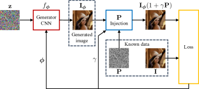
Figure 1: The proposed DIP-based image generation process. The known data are the acquired image $\mathbf{I}$ and the device fingerprint $\mathbf{P}$. During the inversion, the traces of $\mathbf{P}$ are attenuated by injecting $\mathbf{P}$ into the image $\mathbf{I}_{\bm{\phi}}$ generated by the CNN. In the PRNU-aware setup, $\mathbf{P}=\mathbf{K}$; in the PRNU-blind setup, $\mathbf{P}=\mathbf{W}$, a noise residual extracted from $\mathbf{I}$ [2].

3.2 Generation of PRNU-attenuated images

As we previously reported, the proposed DIP process can generate multiple images with attenuated PRNU traces. Referring to Figure 1, the generation pipeline is the following:

1. The CNN input tensor $\mathbf{z}$ is a realization of a zero-mean white gaussian noise, with the same size of image $\mathbf{I}$. We found uniform distributions to be less effective; we are convinced the white gaussian noise is able to excite a broader frequency range and can produce better images.

2. We optimize the weights of the CNN by minimizing (9). The optimization is performed over the generator weights $\bm{\phi}$. Notice that the PRNU injection weight $\gamma$ acts as a trainable layer of the architecture, so $\gamma$ is estimated directly during the inversion. Specifically, $\gamma$ is clamped to be positive, as negative $\gamma$ values are not model representative.

3. At each minimization step, we generate an image $\mathbf{I}_{\bm{\phi}}$, which is saved only if the PSNR with respect to the original image $\mathbf{I}$ is above a certain threshold $\tau_{\textrm{PSNR}}$. This is done to guarantee a sufficiently good visual quality for the generated image.

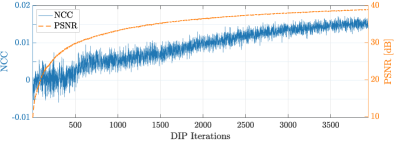
Figure 2: NCC and PSNR behaviour of generated images as a function of DIP iterations. Some generated images are depicted in Figure 3.

The minimization process ends when the PSNR between the generated image $\mathbf{I}_{\bm{\phi}}$ and the initial image $\mathbf{I}$ overcomes a threshold of $39\textrm{dB}$. The maximum number of iterations is anyway fixed to $10000$. In doing so, after the DIP process ends, a pool of $M$ generated images ${\mathbf{I}_{\bm{\phi}}}^{(m)},m\in[1,M]$ with PSNR $\geq\tau_{\textrm{PSNR}}$ has been collected. For the sake of clarity, Figure 2 and Figure 3 report one example of the inversion process, showing the evolution of the CNN-generated images, together with their PSNRs with respect to the original image and NCCs with the source device PRNU.

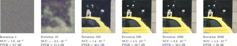
Figure 3: DIP inversion example: as iterations increase, the reconstructed images pass from a noisy behaviour (i.e., iteration $1$) to a very similar copy of the original image. However, as PSNR, NCC can slightly grow as well.

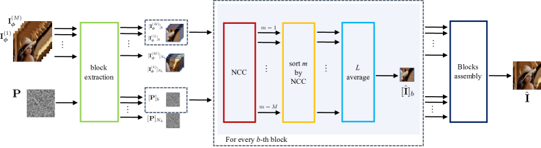
Figure 4: Assembly of the anonymized image. For each generated image ${\mathbf{I}_{\bm{\phi}}}^{(m)}$, $N_{b}$ blocks are extracted from the image and the fingerprint $\mathbf{P}$. Fixing a block position $b$, we compute the NCC between each pair of blocks $[{\mathbf{I}_{\bm{\phi}}}^{(m)}]_{b}$, $[\mathbf{P}]_{b}$, $m\in[1,M]$. Then, we order the $M$ image blocks according to their resulting NCCs and we average the first $L$ blocks pixel by pixel, obtaining the estimated block $[{\hat{\mathbf{I}}}]_{b}$. We follow this pipeline for each block position $b$, eventually assembling the results and estimating the anonymized image ${\hat{\mathbf{I}}}$.

3.3 Local post-processing and assembly

Notice that the DIP minimization functional Equation 9 imposes a constraint on the Frobenius norm of the difference between the fingerprint-injected image and the initial image. This constraint represents a global constraint as it does not specifically focus on local pixel areas. Recalling our final goals (i.e., maximizing the PSNR and minimizing the NCC of the anonymized image), while the PSNR is a global metrics as it considers the entire image and not local areas, the NCC can strongly depend on specific local regions of the image which can correlate with the device PRNU in diverse fashions.

Moreover, as DIP iterations increase, the minimization process risks to inject an excessive amount of PRNU traces in the generated images. This is noticeable from the examples depicted in Figure 2 and Figure 3: when iterations’ number grows, the PSNR of the generated images improves but their NCC can slightly grow as well, resulting in worse anonymization.

Given these premises, we propose to further optimize our solution by investigating the $M$ generated images on their local areas. We improve upon these results with a very straightforward methodology to generate one final anonymized image out of the $M$ previously generated, by locally optimizing the cross-correlation with the reference device fingerprint $\mathbf{P}$.

Specifically, Figure 4 depicts the proposed pipeline: we divide each available image ${\mathbf{I}_{\bm{\phi}}}^{(m)}$ and the reference fingerprint $\mathbf{P}$ into $N_{b}$ non overlapping squared blocks of $B\times B$ pixels. Image and fingerprint blocks are defined as $[{\mathbf{I}_{\bm{\phi}}}^{(m)}]_{b}$ and $[\mathbf{P}]_{b},b\in[1,N_{b}]$, respectively. Notice that, for each block geometric position $b$, we have $M$ available image blocks associated with the $M$ image realizations produced during the DIP iterations. For each block position $b$, three main steps follow:

1. We compute the NCCs between the $M$ image blocks $[{\mathbf{I}_{\bm{\phi}}}^{(m)}]_{b},m\in[1,M]$ and the fingerprint block $[\mathbf{P}]_{b}$ as in (2).

2. The available $M$ blocks are ordered accordingly to their resulting NCCs: first, we select the blocks with negative NCC and increasing absolute value; secondly, we select the blocks with positive NCC and increasing absolute value. In doing so, blocks with low absolute value of NCC and negative NCC are given higher priority than blocks returning bigger NCCs.

3. Following the order specified above, we average the first $L$ blocks pixel by pixel, ending up with a $B\times B$ final reconstructed block.

The final anonymized image $\hat{\mathbf{I}}$ is estimated by assembling the results obtained for each single block position $b$ and color channel.

3.4 CNN Architecture

The U-Net is a convolutional autoencoder (i.e., a CNN aiming at reconstructing a processed version of its input) characterized by the so called skip-connections and originally introduced for medical image processing [22]. If properly trained according to the standard deep learning paradigm, it proves very effective for multidimensional signal processing tasks such as denoising [23, 24], interpolation [25, 26], segmentation [27, 28], inpainting [29], and domain-specific post-processing operators [30, 31].

More recently, the Multi-Resolution U-Net [32] has been proposed for multimodal medical image segmentation, based on the consideration that the targets of interest have different shapes and scales. If we want to capture self-similarities of natural images to be employed as a prior, working at different scales can be strongly beneficial. Preliminary experiments on a small dataset led us to adopt such architecture rather than traditional U-Net and its derivations analyzed in [14].

Therefore, we propose an ad-hoc Multi-Resolution U-Net (shown in Figure 5) that can be summarized as follows:

1. Convolutional layers are replaced by so called Multi Resolution blocks shown in the bottom-right portion of Figure 5. These blocks approximate multi-scale features of the Inception block [33] while limiting the number of parameters of the network, which is critical when employing it as a deep prior. Every block is a chain of three convolutions; the final output is the sum of the input, scaled by a learned factor, and the stack of the three partial outputs.

2. Skip connections, which are the distinctive feature of the U-Net, are replaced by Residual Path blocks shown in the bottom-left portion of Figure 5, as proposed in [32]. $\mathcal{E}$ is the output of an encoding layer and $\mathcal{D}$ is concatenated to the corresponding decoding layer.

3. Downsampling is achieved by $3\times 3$ convolutions with stride $2\times 2$. Upsampling is performed by nearest neighbor interpolation. Batch Normalization and LeakyReLU activation follow every convolution apart from the last one (i.e., the CNN output) that is activated by a sigmoid.

Notice that, even though the result is the output of a CNN, the DIP method does not exploit the typical deep learning paradigm where a training phase is performed over a specifically designed set of data. In particular, only the query image is used in the reconstruction process and the CNN implicitly assumes the role of prior information that exploits correlations in the image to learn its inner structure.

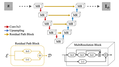
Figure 5: Proposed Multi-Resolution U-Net architecture.

4 Experiments

In this section, we describe the used datasets, the experimental setup and the evaluation metrics.

4.1 Datasets

We resort to two well-known datasets, commonly used for investigating PRNU-related problems on images. The first dataset is the Dresden Image Database [15], which collects both uncompressed and compressed images from more than $50$ diverse devices. Following the same procedure done in past works proposed in literature [13, 12], we select images from $6$ different camera instances, precisely Nikon D70, Nikon D70s, Nikon D200, two devices each. Second dataset is the recently released Vision Dataset [16], which includes JPEG compressed images captured from $35$ devices. Among the pool of available models, we collect images from $6$ different camera vendors, precisely from devices named as D12, D17, D19, D21, D24, D27 in [16].

The PRNU fingerprint of each device is computed by collecting all the available flat-field images shot by the device and following the Maximum Likelihood estimation proposed in [2]. Concerning the Dresden dataset, we exploit never-compressed Adobe Lightroom images to compute the PRNU, as it reasonably is the most accurate way to estimate the device fingerprint. Indeed, JPEG compression can create blockiness artifacts that may hinder PRNU estimation [2]. Every device includes $25$ homogeneously lit flat-field images for the PRNU estimation. For Vision dataset, we have more than $95$ JPEG flat-content images to compute each device fingerprint.

The images to be anonymized are selected from natural images, precisely we pick $100$ natural images per device. Regarding Dresden dataset, two different sub-sets can be extracted: for every device, we select $100$ never-compressed Adobe Lightroom images, together with other $100$ taken from the pool of JPEG compressed images. We end up with three distinct datasets comprising $600$ images each: the Dresden uncompressed dataset, called $\mathcal{D}_{u}$; the Dresden compressed dataset, defined as $\mathcal{D}_{c}$; the Vision (compressed) dataset, $\mathcal{V}$.

4.2 State-of-the-arst solutions

As state-of-the-art solutions, we select the most recent anonymization methods proposed in the literature.

Among the pool of PRNU-aware methods, we implement the method proposed in [6], being the most recent and cited contribution. We do not compare our solution with the PRNU-aware strategy recently proposed in [8], as its performance drops significantly whenever the used image denoising operator during cross-correlation tests is the commonly used one suggested in [1, 2]. Since in our proposed strategy we follow the methodology devised in [1, 2] for image denoising and cross-correlation, a comparison with [8] would be unfair.

Regarding PRNU-blind strategies, the most recent contribution is that proposed by us in [13], which demonstrates to outperform results of [12] in a PRNU-blind scenario. For the implementation of [13], we consider the parameter configurations achieving the best anonymization results, i.e., the strategies defined as $\ell^{(3)}_{1}$ and $\ell^{(5)}_{1}$ in the original paper.

Moreover, to show that simple denoising does not achieve good anonymization performances [10], we implement the well-known DnCNN denoiser [23] which represents a modern data-driven solution among image denoising strategies.

4.3 Experimental Setup

Considering what was done in the past state-of-the-art [13], our experiments process images of $512\times 512$ pixels with $512$ features extracted at the first MultiRes block. To do so, we center-crop all the images and the computed PRNUs to a common resolution of $512\times 512$ pixels. The optimization is performed through ADAM algorithm with learning rate $0.001$. At each iteration, we perturb the CNN input noise $\mathbf{z}$ with additive white gaussian noise with standard deviation $0.1$ to strengthen the convergence. This way, the network is more robust with respect to the specific noise realization and it is forced to learn higher level features. Without any specific code optimization, we reach a computation speed of $5$ iterations per second on a Nvidia Tesla V100 GPU, requiring $8$ GB of GPU memory.

Concerning the proposed local post-processing and assembly in Section 3.3, notice that the amount of $M$ available images at the output of DIP process changes accordingly to the input image, and to the PSNR requirement. Typical values are between 500 and 2500 images. The computational impact of the post-processing is mainly due to the Wiener filter that estimates the noise residual on all the $M$ images.. It is worth noticing that the vast majority of images needs few iterations (less than $3000$ iterations over $10000$ possible cycles, on average) to achieve the threshold of $39\textrm{dB}$ chosen to stop the inversion. We consider multiple parameter configurations in order to include a sufficiently wide pool of investigation cases. The block size $B$ can be chosen among $B=[32,64,128,256,512]$ pixels, and the maximum number of averaged blocks can vary as well, being $L=[1,5,10,25,50,75,100]$. Notice that the case $B=512$ corresponds to select the full image, without dividing it into blocks. It is worth noticing that the configuration $\{L=1,B=512\}$ coincides with the absence of the local area post-processing proposed in Section 3.3.

4.4 Evaluation Metrics

After the generation of the anonymized image $\hat{\mathbf{I}}$, we compute the NCC between $\hat{\mathbf{I}}$ and the source device PRNU $\mathbf{K}$, together with the PSNR between $\hat{\mathbf{I}}$ and the original image $\mathbf{I}$. These values are the used metrics for evaluating the results and comparing with state-of-the-art. The lower the achieved NCC together with a high PSNR, the better the image anonymization performance.

To summarize results related to the achieved NCCs, we make use of Receiver Operating Characteristic (ROC) curves related to the source device identification problem. Given a fixed device PRNU $\mathbf{K}$, NCCs of anonymized images taken with that device are defined as the positive set, while NCCs of images shot by other cameras are the negative set. Anonymization performance is evaluated through the Area Under the Curve (AUC), as done in [12, 13, 8]. Our goal is to reduce the AUC of the curves, thus making the PRNU-based identification not working, at the same time maintaining high values of PSNR.

5 Results and Discussion

In this section we provide the numerical results achieved with our experimental campaign that demonstrate the capability and limitations of our methodology. First, we deploy our method when the reference PRNU of the device is available at the analyst (i.e., $\mathbf{P}=\mathbf{K})$. Then, we show that our method can also be applied in the case of blind anonymization when the PRNU $\mathbf{K}$ is unknown (i.e., $\mathbf{P}=\mathbf{W})$. Results are compared with state-of-the-art techniques to highlight pros and cons.

5.1 PRNU-aware anonymization

In this scenario, the actual PRNU of the source device to be anonymized is known. Results are shown in terms of PSNR and AUC of the ROC curves for the three investigated datasets. Figure 6, Figure 7, Figure 8 refer to datasets $\mathcal{D}_{u}$, $\mathcal{D}_{c}$ and $\mathcal{V}$, respectively. For the sake of clarity in the following discussion, results for $L=25$ and $L=75$ are not depicted in these plots. It is important to notice that results must be analyzed by watching PSNR and AUC concurrently. Indeed, high PSNR is a good result only if paired with low AUC. We therefore privilege solutions providing a good PSNR / AUC trade-off. To ease the readability of reported results, we separately analyze in brief paragraphs the performance of each PRNU-anonymization method.
Proposed DIPPAS method. For all the investigated datasets, the proposed method is able to achieve PSNRs greater than $38$ dB, provided that a sufficiently high threshold $\tau_{\textrm{PSNR}}$ is chosen. Also in terms of AUCs, the proposed method can cover a wide range of possibilities, according to the chosen block size $B$ and amount of averaged blocks $L$. It is worth noticing that the application of local post-processing presented in Section 3.3 allows an improvement of the results in all the three scenarios. The DIP approach alone, which corresponds to configuration $\{L=1,B=512\}$, often shows low PSNRs and too high AUCs. Instead, by working on smaller image blocks, both PSNR and AUC improve, even without averaging multiple blocks together (i.e., with $L=1$).

In general, the smaller the block size $B$, the better the PSNR achieved, even though this behaviour seems to attenuate for high values of $\tau_{\textrm{PSNR}}$. Besides, the more the amount of averaged blocks $L$, the better the achieved PSNR. Regarding Dresden-related datasets, middle values of $L$ seem to work better for achieving good AUCs, while dataset $\mathcal{V}$ requires higher values of $L$ for lowering the AUC. The achieved AUCs are better on Dresden-related datasets, i.e., Figure 6 and Figure 7. For these two datasets, none of the state-of-the-art works outperforms the best DIPPAS results, while $\mathcal{V}$ dataset seems to be more challenging to be anonymized.
Proposed method in [6]. The solution provided by [6] achieves the best results in terms of PSNR for all three datasets. However, notice that the corresponding AUCs show very poor results if compared with DIPPAS and [13] for Dresden-related datasets. Concerning the dataset $\mathcal{V}$ shown in Figure 8, the AUC obtained by [6] seems to outperform every proposed strategy.

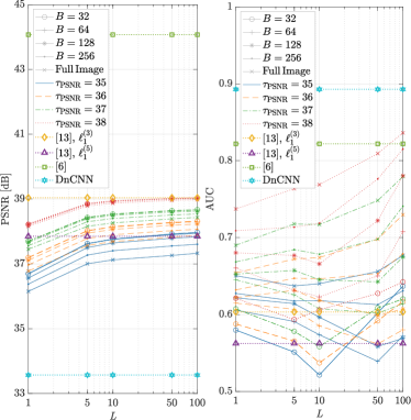
Figure 6: PRNU-aware anonymization results for the $\mathcal{D}_{u}$ dataset.

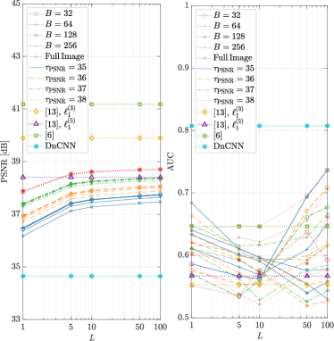
Figure 7: PRNU-aware anonymization results for the $\mathcal{D}_{c}$ dataset.

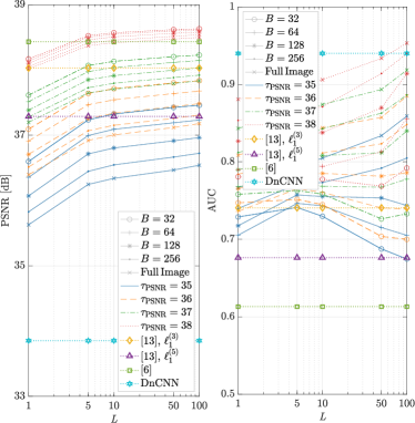
Figure 8: PRNU-aware anonymization results for the $\mathcal{V}$ dataset.

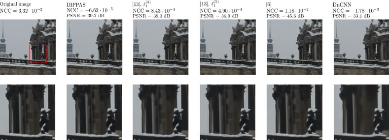
Figure 9: PRNU-aware anonymization for an image of the $\mathcal{D}_{c}$ dataset, comparing our proposed strategy with [13], [6] and DnCNN.

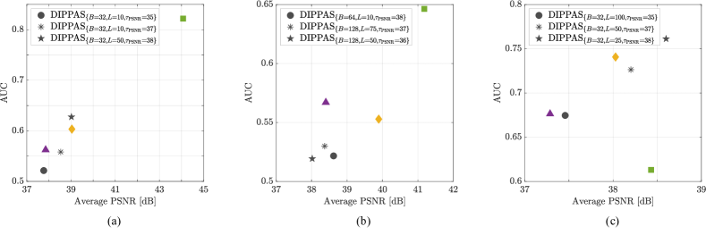
Figure 10: PRNU-aware anonymization results, reported in terms of AUC as a function of average PSNR achieved by three DIPPAS configurations for (a): the $\mathcal{D}_{u}$ dataset, (b): the $\mathcal{D}_{c}$ dataset, (c): the $\mathcal{V}$ dataset. We compare our proposed strategy with [13] $\ell_{1}^{(3)}$ (yellow $\blacklozenge$), [13] $\ell_{1}^{(5)}$ (purple $\blacktriangle$) and [6] (green $\blacksquare$).

We think this different behaviour can be explained by the diverse nature of Vision dataset with respect to Dresden. Indeed, in dataset $\mathcal{V}$ the device PRNU is estimated directly from JPEG-compressed images, while in Dresden-based datasets the PRNU is estimated from uncompressed ones. As a matter of fact, the PRNU estimated from JPEG-compressed images can present artifacts due to JPEG compression, which can also contribute to hinder the subtle sensor traces left on images [2]. As a consequence, anonymizing JPEG-compressed images with respect to the PRNU estimated from uncompressed data can be slightly more complicated than anonymizing JPEG images with respect to the PRNU estimated from JPEG data. In this vein, the strategy proposed by [6] seems to work in a very accurate way only if the device PRNU is estimated from JPEG-compressed images.
Proposed method in [13]. The proposed strategy in [13] achieves acceptable values of PSNRs in all the considered datasets, actually comparable to those achieved by DIPPAS. The resulting AUCs show satisfying values as well, except for the Vision-related dataset, where [13] seems to suffer more with respect to Dresden-related datasets, following a similar trend to that previously shown by DIPPAS method. Regardless, notice that DIPPAS can outperform the AUCs achieved by [13] in all three datasets.
Proposed method in [23]. The DnCNN solution proposed in [23] shows small values of PSNRs in all the experiments. Furthermore, the achieved results report too high AUCs, actually unacceptable for satisfactory image anonymization. DnCNN results seem to confirm that this simple image denoiser cannot accurately delete PRNU traces [10], leading to poor anonymization performances.

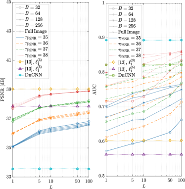
Figure 11: PRNU-blind anonymization results for the $\mathcal{D}_{u}$ dataset.

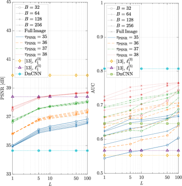
Figure 12: PRNU-blind anonymization results for the $\mathcal{D}_{c}$ dataset.

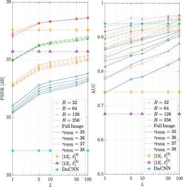
Figure 13: PRNU-blind anonymization results for the $\mathcal{V}$ dataset.

Figure 9 reports an example of anonymization performed over an image of $\mathcal{D}_{c}$ dataset. We depict the original image and its anonymized versions exploiting DIPPAS and the methods of [13], [6] and DnCNN [23]. Specifically, we choose the best performing DIPPAS parameter configuration in terms of both PSNR and AUC, i.e., $\{\tau_{\textrm{PSNR}}=38,B=64,L=10\}$; we select this configuration by referring to results shown in Figure 7. Zooming in the images (red squared area), we can visually notice that the best results are obtained by DIPPAS and [6]; DnCNN results in a heavily smoothed image, while [13] introduces some edge artifacts. The method devised in [6] is able to halve the original NCC, while DIPPAS dramatically scales the original NCC value by a factor of $0.002$.

To summarize the previously reported results, Figure 10 shows the behaviour of AUC as a function of the average PSNR achieved by DIPPAS in three selected parameter configurations. We compare our results with state-of-the-art as well. The best working condition consists in high PSNR and low AUC. It is possible to notice that DIPPAS provides the best trade-off on Dresden dataset, and the second best one on Vision. In this latter scenario, the best trade-off is provided by [6], which however reports very poor results on Dresden dataset.

5.2 PRNU-blind anonymization

In this scenario, the actual device PRNU is unknown, therefore the reference device fingerprint used during the DIP inversion and the blocks assembly corresponds to the noise residual extracted from the image, i.e., $\mathbf{P}=\mathbf{W}$. As previously done, we report the PSNR and AUC of the ROC curves for all three investigated datasets. Figure 11, Figure 12, Figure 13 depicts results for datasets $\mathcal{D}_{u}$, $\mathcal{D}_{c}$ and $\mathcal{V}$, respectively. For the sake of clarity in the following discussion, results for $L=25$ and $L=75$ are not depicted in these plots.

In terms of PSNR, on Vision dataset we are able to outperform [13], while for Dresden dataset we achieve slightly lower results. Moreover, DIPPAS achieves slightly higher AUCs than state-of-the-art solutions. Notice that the best AUC values are obtained for $L=1$, i.e., without performing block averaging.

We think this less effective anonymization with respect to the previous PRNU-aware scenario can be due to the assumption done during the DIP inversion (9) in order to estimate the anonymized image. As a matter of fact, the DIP paradigm leverages the PRNU-based image modeling reported in (1). Whenever the PRNU estimate $\mathbf{K}$ is unknown and the noise residual $\mathbf{W}$ is used instead, as reported in (11), the model is not clearly satisfied and the DIP solution will be sub-optimum. For this reason, in a PRNU-blind scenario, DIPPAS is still able to achieve good performance in terms of PSNR, but the AUC is not as good as in the PRNU-aware scenario.

From these results it may seem that DIPPAS cannot achieve better results than [13], but an important point has to be noticed. Indeed, [13] applies different processing to edges and to flat regions, thus removing PRNU traces in concentrated local regions. Precisely, notice that method [13] works in two separate steps: (i) estimate an anonymized version of the image exploiting inpainting techniques; (ii) substitute a denoised version of the edges extracted from the original image into the anonymized image, in order to enhance the output visual quality. In light of these considerations, we think that the edge processing operation performed on the output image can be the weak link in the proposed pipeline of [13]. Indeed, image edges only undergo two successive steps of BM3D denoising algorithm [34], thus they reasonably contain enough PRNU traces for performing source attribution, as suggested in [10].

Therefore, we compare DIPPAS and [13] only along the image edges, extracted following the same pipeline proposed in [13]. For every dataset, we evaluate DIPPAS results for a parameter configuration which returns the nearest PSNR value to that achieved by [13]. For instance, looking at Figure 11, dataset $\mathcal{D}_{u}$ is evaluated for $\{B=32,L=100,\tau_{\textrm{PSNR}}=38\}$ if compared to [13], $\ell_{1}^{(3)}$; we use $\{B=512,L=10,\tau_{\textrm{PSNR}}=37\}$ when comparing to [13], $\ell_{1}^{(5)}$.

We compare results in terms of relative change of AUC evaluated over image edges with respect to the AUC achieved on the full image. In a nutshell, the relative change in AUC can be computed as $(\textrm{AUC}_{\text{edges}}-\textrm{AUC})/{\textrm{AUC}}$, being AUC the metrics associated to the full image. Table 1 reports the results. Notice that the relative AUC change maintains a coherent behaviour for all the three datasets. On one side, [13] always reports a positive relative change; on the other side, DIPPAS presents a negative relative change.

DIPPAS results are coherent with what actually happens on natural images when compared with the PRNU in a reduced region (e.g., only along the edges). Indeed, the NCC drops as the image content is reduced, thus the AUC of the source attribution problem decreases. On the contrary, accuracy of [13] evaluated only along image edges strongly drops as the NCC increases, with a consequent AUC growth. This phenomenon can be explained by the previously reported consideration, that is, [13] performs only denoising along the edges and this is usually not enough to hinder PRNU traces [10].

As a consequence, the anonymization algorithm proposed in [13] can be easily spotted and defeated just by analyzing image edges, whereas the DIPPAS proposed solution does not present this drawback. Even if an analyst only use edges for PRNU-based attribution, the image would look anonymized. This is an additional pro of DIPPAS technique.

Table 1: AUC relative change on image edges, for prnu-blind anonymization.

NCC area	[13], $\ell^{(3)}_{1}$	DIPPAS
$\mathcal{V}_{\textrm{edges}}$	$+11.6\%$	$-9.1\%$
$\mathcal{D}_{u_{\textrm{edges}}}$	$+10.9\%$	$-17.8\%$
$\mathcal{D}_{c_{\textrm{edges}}}$	$+8.7\%$	$-17.6\%$

NCC area	[13], $\ell^{(5)}_{1}$	DIPPAS
$\mathcal{V}_{\textrm{edges}}$	$+22.3\%$	$-9.9\%$
$\mathcal{D}_{u_{\textrm{edges}}}$	$+19.1\%$	$-19.1\%$
$\mathcal{D}_{c_{\textrm{edges}}}$	$+6.1\%$	$-17.7\%$

6 conclusions

In this manuscript, we propose a source device anonymization scheme that leverages the Deep Image Prior (DIP) paradigm to attenuate PRNU traces in natural images, paired with a post-processing scheme that exploits multiple images. With this method, a CNN learns to iteratively generate images from noise realizations. Specifically, at each DIP iteration: (i) the CNN generates an image; (ii) we inject the device PRNU into this image; (iii) we minimize the distance between the input query image and the PRNU-injected image. In doing so, we are able to generate multiple images with a strongly attenuated PRNU pattern and high visual quality. Finally, we devise an efficient post-processing operation for assembling the final anonymized image from the CNN outputs realized at different iterations.

We compare our method against state-of-the-art anonymization schemes through numerical examples. In particular, when the PRNU of the device is available, we achieve our best results. Our scheme can be generalized to the case of blind anonymization, i.e., when the device PRNU is unknown and only a noise residual can be extracted from the query image and then injected into the DIP generation process.

Not surprisingly, our method suffers when the injected noise is quite different from the source device PRNU. However, it still proves interesting when compared to state-of-the-art solutions if we consider the homogeneity of PRNU removal effect. Indeed, we are capable of removing PRNU traces on all image regions, whereas the considered baseline leaves image edges mainly non-anonymized.

Our future work will be devoted to investigate the possibility of starting from a pre-trained network to speed-up convergence. Moreover, we will focus on a better inversion model to be used in case of blind PRNU removal.

Availability of supporting data

All the numeric experiments shown in this manuscript relies on publicly available datasets [15, 16]. The codes have been released in a GitHub repository at: https://github.com/polimi-ispl/dip_prnu_anonymizer.

Competing interests

The authors declare that they have no competing interests.

Funding

The authors have no funding to be declared.

Author’s contributions

All authors contributed in the design of the proposed method and writing the manuscript.

References

- [1] Lukáš, J., Fridrich, J., Goljan, M.: Digital camera identification from sensor pattern noise. IEEE Transactions on Information Forensics and Security (TIFS) 1, 205–214 (2006)
- [2] Chen, M., Fridrich, J., Goljan, M., Lukas, J.: Determining image origin and integrity using sensor noise. IEEE Transactions on Information Forensics and Security (TIFS) 3, 74–90 (2008)
- [3] Kirchner, M., Johnson, C.: SPN-CNN: Boosting Sensor-Based Source Camera Attribution with Deep Learning. In: IEEE International Workshop on Information Forensics and Security (2019)
- [4] Mandelli, S., Cozzolino, D., Bestagini, P., Verdoliva, L., Tubaro, S.: Cnn-based fast source device identification. IEEE Signal Processing Letters 27, 1285–1289 (2020)
- [5] Chen, M., Fridrich, J., Goljan, M., Lukas, J.: Source digital camcorder identification using sensor photo-response nonuniformity. In: SPIE Electronic Imaging (EI) (2007)
- [6] Karaküçük, A., Dirik, A.E.: Adaptive photo-response non-uniformity noise removal against image source attribution. Journal of Digital Investigation 12, 66–76 (2015)
- [7] Zeng, H., Chen, J., Kang, X., Zeng, W.: Removing camera fingerprint to disguise photograph source. In: IEEE International Conference on Image Processing (ICIP) (2015)
- [8] Bonettini, N., Bondi, L., Güera, D., Mandelli, S., Bestagini, P., Tubaro, S., Delp, E.J.: Fooling prnu-based detectors through convolutional neural networks. In: 2018 26th European Signal Processing Conference (EUSIPCO), pp. 957–961 (2018). IEEE
- [9] Rosenfeld, K., Sencar, H.T.: A study of the robustness of PRNU-based camera identification. In: IS&T/SPIE Electronic Imaging (EI) (2009). International Society for Optics and Photonics
- [10] Bernacki, J.: On robustness of camera identification algorithms. Multimedia Tools and Applications, 1–22 (2020)
- [11] Dirik, A.E., Sencar, H.T., Memon, N.: Analysis of seam-carving-based anonymization of images against PRNU noise pattern-based source attribution. IEEE Transactions on Information Forensics and Security (TIFS) 9, 2277–2290 (2014)
- [12] Entrieri, J., Kirchner, M.: Patch-based desynchronization of digital camera sensor fingerprints. In: IS&T Electronic Imaging (EI) (2016)
- [13] Mandelli, S., Bondi, L., Lameri, S., Lipari, V., Bestagini, P., Tubaro, S.: Inpainting-based camera anonymization. In: IEEE International Conference on Image Processing (ICIP) (2017)
- [14] Ulyanov, D., Vedaldi, A., Lempitsky, V.: Deep image prior. In: The IEEE Conference on Computer Vision and Pattern Recognition (CVPR) (2018)
- [15] Gloe, T., Böhme, R.: The dresden image database for benchmarking digital image forensics. Journal of Digital Forensic Practice 3, 150–159 (2010)
- [16] Shullani, D., Fontani, M., Iuliani, M., Shaya, O.A., Piva, A.: Vision: a video and image dataset for source identification. EURASIP Journal on Information Security 15 (2017)
- [17] Moulin, P., Juan Liu: Analysis of multiresolution image denoising schemes using generalized gaussian and complexity priors. IEEE Transactions on Information Theory 45(3), 909–919 (1999). doi:10.1109/18.761332
- [18] Tirer, T., Giryes, R.: Back-projection based fidelity term for ill-posed linear inverse problems. IEEE Transactions on Image Processing 29, 6164–6179 (2020). doi:10.1109/TIP.2020.2988779
- [19] Dong, W., Wang, P., Yin, W., Shi, G., Wu, F., Lu, X.: Denoising prior driven deep neural network for image restoration. IEEE Transactions on Pattern Analysis and Machine Intelligence 41(10), 2305–2318 (2019). doi:10.1109/TPAMI.2018.2873610
- [20] Lin, B., Tao, X., Lu, J.: Hyperspectral image denoising via matrix factorization and deep prior regularization. IEEE Transactions on Image Processing 29, 565–578 (2020). doi:10.1109/TIP.2019.2928627
- [21] Aggarwal, H.K., Mani, M.P., Jacob, M.: Modl: Model-based deep learning architecture for inverse problems. IEEE Transactions on Medical Imaging 38(2), 394–405 (2019). doi:10.1109/TMI.2018.2865356
- [22] Ronneberger, O., Fischer, P., Brox, T.: U-net: Convolutional networks for biomedical image segmentation. In: International Conference on Medical Image Computing and Computer-assisted Intervention, pp. 234–241 (2015). Springer
- [23] Zhang, K., Zuo, W., Chen, Y., Meng, D., Zhang, L.: Beyond a gaussian denoiser: Residual learning of deep cnn for image denoising. IEEE Transactions on Image Processing (TIP) 26(7), 3142–3155 (2017). doi:10.1109/TIP.2017.2662206
- [24] Cruz, C., Foi, A., Katkovnik, V., Egiazarian, K.: Nonlocality-reinforced convolutional neural networks for image denoising. IEEE Signal Processing Letters 25(8), 1216–1220 (2018). doi:10.1109/LSP.2018.2850222
- [25] Kong, F., Picetti, F., Lipari, V., Bestagini, P., Tubaro, S.: Deep prior-based seismic data interpolation via multi-res u-net. In: SEG Technical Program Expanded Abstracts 2020, pp. 3159–3163 (2020). doi:10.1190/segam2020-3426173.1
- [26] Mandelli, S., Borra, F., Lipari, V., Bestagini, P., Sarti, A., Tubaro, S.: Seismic data interpolation through convolutional autoencoder. In: SEG Technical Program Expanded Abstracts 2018, pp. 4101–4105 (2018). doi:10.1190/segam2018-2995428.1
- [27] Zhou, Z., Siddiquee, M.M.R., Tajbakhsh, N., Liang, J.: Unet++: Redesigning skip connections to exploit multiscale features in image segmentation. IEEE Transactions on Medical Imaging 39(6), 1856–1867 (2020). doi:10.1109/TMI.2019.2959609
- [28] Jurdi, R.E., Petitjean, C., Honeine, P., Abdallah, F.: Bb-unet: U-net with bounding box prior. IEEE Journal of Selected Topics in Signal Processing 14(6), 1189–1198 (2020). doi:10.1109/JSTSP.2020.3001502
- [29] Sidorov, O., Hardeberg, J.Y.: Deep hyperspectral prior: Single-image denoising, inpainting, super-resolution. In: 2019 IEEE/CVF International Conference on Computer Vision Workshop (ICCVW), pp. 3844–3851 (2019). doi:10.1109/ICCVW.2019.00477
- [30] Picetti, F., Lipari, V., Bestagini, P., Tubaro, S.: Seismic image processing through the generative adversarial network. Interpretation 7(3), 15–26 (2019). doi:10.1190/INT-2018-0232.1
- [31] Devoti, F., Parera, C., Lieto, A., Moro, D., Lipari, V., Bestagini, P., Tubaro, S.: Wavefield compression for seismic imaging via convolutional neural networks. In: SEG Technical Program Expanded Abstracts 2019, pp. 2227–2231 (2019). doi:10.1190/segam2019-3216395.1
- [32] Ibtehaz, N., Rahman, M.S.: Multiresunet: Rethinking the u-net architecture for multimodal biomedical image segmentation. Neural Networks 121, 74–87 (2020)
- [33] Szegedy, C., Liu, W., Jia, Y., Sermanet, P., Reed, S., Anguelov, D., Erhan, D., Vanhoucke, V., Rabinovich, A.: Going deeper with convolutions. In: Proceedings of the IEEE Conference on Computer Vision and Pattern Recognition (CVPR) (2015)
- [34] Dabov, K., Foi, A., Katkovnik, V., Egiazarian, K.: Image denoising by sparse 3D transform-domain collaborative filtering. IEEE Transactions on Image Processing (TIP) 16, 2080–2095 (2007)