Fine-grained Angular Contrastive Learning with Coarse Labels

Abstract

Few-shot learning methods offer pre-training techniques optimized for easier later adaptation of the model to new classes (unseen during training) using one or a few examples. This adaptivity to unseen classes is especially important for many practical applications where the pre-trained label space cannot remain fixed for effective use and the model needs to be ”specialized” to support new categories on the fly. One particularly interesting scenario, essentially overlooked by the few-shot literature, is Coarse-to-Fine Few-Shot (C2FS), where the training classes (e.g. animals) are of much ‘coarser granularity’ than the target (test) classes (e.g. breeds). A very practical example of C2FS is when the target classes are sub-classes of the training classes. Intuitively, it is especially challenging as (both regular and few-shot) supervised pre-training tends to learn to ignore intra-class variability which is essential for separating sub-classes. In this paper, we introduce a novel ’Angular normalization’ module that allows to effectively combine supervised and self-supervised contrastive pre-training to approach the proposed C2FS task, demonstrating significant gains in a broad study over multiple baselines and datasets. We hope that this work will help to pave the way for future research on this new, challenging, and very practical topic of C2FS classification.

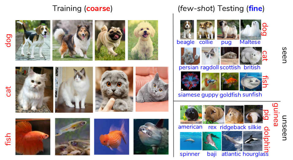
Figure 1: The Coarse-to-Fine Few-Shot (C2FS): During training we observe only coarse class labels (in red, e.g. animals), while at test time we are expected to adapt our model to support the fine classes (in blue, e.g. breeds) using one or few samples. The fine classes may be sub-classes of the train classes (seen) or sub-classes of classes unseen during training.

1 Introduction

In the most commonly encountered learning scenario, supervised learning, a set of target (class) labels is provided for a set of samples (images) using which we train a model (CNN [26, 18, 53] or Transformer [66, 40]) that casts these samples into some representation space from which predictions are made, e.g. using a linear classifier. Nevertheless, while supervised learning is a very common setting, in many practical applications the set of the target labels of interest is not static, and may change over time. One good example is few-shot learning [57, 49, 55], where a model is pre-trained in such a way that more classes could be added later with only very few additional labeled examples used for adapting the model to support these new classes.

However, in previous few-shot learning works most (if not all) of the new classes: (i) are separate from the classes the model already knows, in the sense that they either belong to a different branch of the class hierarchy or are siblings to the known classes; and (ii) are of same or similar level of granularity (same level of class hierarchy). But what about the very practical situation when the new classes are fine-grained sub-classes strictly included inside the known (coarse) classes being their descendants in the class taxonomy? This situation typically occurs during the lifespan of the model when the application requires separating some sub-classes of the current classes into separate classes and yet when the training dataset was created these (unknown in advance) sub-classes were not annotated. For example, this could occur in product specialization for product search, or during personalizing a generic model to a specific customer. Naturally, going back to re-labeling each time this occurs is much too costly to be an option.

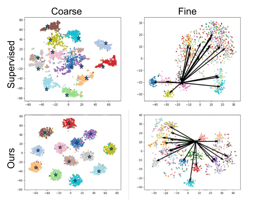
Figure 2: Learned embedding tSNE visualization: Top - coarse-supervised baseline, Bottom - ours (ancor). Left - coarse classes, right - fine sub-classes of one arbitrary coarse class. Stars are embeddings of the linear classifier (class) weight vectors, black arrows point from the class weight to the fine sub-classes centroids. Clearly, ancor induces order on the sub-classes arranging them nicely around the class weight and making them separable.

In this paper, we target the Coarse-to-Fine Few-Shot (C2FS) task (Fig. 1) where a model pre-trained on a set of base classes (denoted as the ‘coarse’ classes), needs to adapt on the fly to an additional set of target (‘fine’) classes of much ‘finer granularity’ than the training classes. The target classes could be sub-classes of the base classes (a particularly interesting case), or they could be a separate set, yet requiring much stronger (than base classes) attention to fine-grained details in order to visually separate. To be efficient, we want this adaptation to occur using only one or few samples of the fine (sub-)classes. Intuitively, this setup is particularly challenging for models pre-trained on the coarse classes in ‘the standard’ supervised manner, as: (a) standard supervised learning losses do not care about the intra-class arrangement of the samples belonging to the same class in the model’s feature space $\mathcal{F}$, as long as these samples are close to each other and the regions associated with different classes are separable (Fig. 2 top-left) - potentially causing the sub-classes to spread arbitrarily inside same-class-associated regions of $\mathcal{F}$ thus hindering their separability (Fig. 2 top-right); and (b) $\mathcal{F}$ is retaining the information on the attributes needed to predict the set of target ‘coarse’ labels, while at the same time reducing intra-class variance and suppressing attributes not relevant to the task for better generalization, which may eliminate the intra-class distinctions between sub-classes (Fig. 2 top-right).

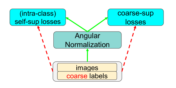
Figure 3: Angular Normalized COntrastive Regularization (ancor): our method jointly employs inter-class supervised and intra-class self-supervised contrastive losses that would pull to different directions without our proposed Angular normalization component that separates the forces applied by the two losses to different planes leading to significant performance gains.

In contrast to supervised learning, recently emerged contrastive self-supervised methods [3, 17, 2, 13] were proven highly instrumental in learning good features without any labels. These methods are able to pre-train effectively attaining almost the same representation (feature) quality as fully supervised counterparts, and even surpassing it when transferring to other tasks (e.g. detection [17]). Even more importantly, these methods are optimizing features for ’instance recognition’, retaining the information for identifying the fine details that separate instances between and within classes in the dataset, and thus likely also retaining features needed for effective sub-class recognition. That being said, contrastive methods have so far been mostly evaluated examining their ability for inter-class separation in a relatively favorable condition of an abundance of unlabeled data (e.g. ImageNet). And yet, naive use of these methods for the C2FS task is sub-optimal. On their own, they lack the use of coarse labels supervision. And when naively used jointly with coarse-supervised losses, their lack of synergy with those losses leads to lower gains (Sec. 4.5.1).

Building upon advances in contrastive self-supervised learning, we propose the Angular Normalized COntrastive Regularization (ancor) approach for the C2FS task. It enables few-shot adaptation to fine-grained (sub-)classes using few examples, while pre-training using only coarse class labels. Our approach (Fig. 3) effectively combines, in a multi-task manner, the supervised pre-training on the coarse classes that ensures inter-class separation, with contrastive self-supervised intra-class learning that facilitates the self-organization and separability of the fine sub-classes in the resulting feature space (Fig. 2 bottom). Our method features a novel angular normalization component that enhances the synergy between the supervised and contrastive self-supervised tasks, minimizing friction between them by separating their forces to different planes. We compare ancor to a diverse set of baselines and ablations, on multiple datasets, both underlining its effectiveness and providing a strong basis for future studies of the proposed C2FS task.

To summarize, our contribution is threefold: (i) we propose the Coarse-to-Fine Few-Shot (C2FS) task of training using only coarse class labels and adapting to support finer (sub-)classes with few (even one) examples; (ii) we propose the ancor approach for C2FS task, based on effective multi-task combination of supervised inter-class and self-supervised intra-class learning, featuring a novel angular normalization component to minimize friction and maximize the synergy between the two tasks; (iii) we offer extensive evaluation and analysis showing the strength of our proposed ancor approach on a variety of datasets and compared to a diverse set of baselines.

2 Related Work

Self-supervised learning. While the onset of deep-learning was pre-dominantly ruled by supervised learning [26, 18, 53], recently many self-supervised representation learning methods have emerged. These works generate different self-induced (pretext) pseudo-labels for unlabeled data and drive the visual feature learning without any external supervision. Earlier works used predicting patch position [7], image colorization [65], jigsaw puzzles [36], image in-painting [38], predicting image rotations [12], and others as pretext tasks. Yet, more recently, [56, 54, 3, 17, 5, 13, 2] have demonstrated the power of contrastive instance discrimination, significantly surpassing previous results and narrowing the gap with supervised methods. SimCLR [3] defined positive pairs as two augmentations of the same image and contrasted them with other images of the same batch. Instead, MoCo [17, 5] contrasted with samples extracted from a dynamic queue produced by a slowly progressing momentum encoder. SWAV [2] uses a clustering objective for computing the contrastive loss, BYOL [13] replaces the contrastive InfoNCE loss with direct regression between positive pairs, essentially removing the need for negative samples, and [59] explores the effect of different contrastive augmentation strategies. Interestingly, contrastive methods have recently shown promising results for domain adaptation [22] and supervised learning [23]. Intuitively, for solving our C2FS task both inter-class (between the coarse classes) and intra-class (within the classes) separation are jointly required. Supervised methods are better at inter-class separation, but are worse in intra-class separation (Fig. 2 top right), while contrastive self-supervised methods are better on intra-class and are worse on inter-class discrimination (Tab. 6). In this paper, we show how to properly combine the two to enjoy the benefits of both.

Few-shot learning. Meta-learning methods, which are very popular in the few-shot literature [57, 49, 51, 28, 10, 30, 67, 41, 35, 45, 4, 48, 37, 64, 63, 9, 27, 16, 62, 19, 32, 8], learn from few-shot tasks (or episodes) rather than from individual labeled samples. Such tasks are small datasets, with a few labeled training (support) examples, and a few test (query) examples. The goal is to learn a model that at test time can be adapted to support novel categories, unseen during training on the base categories (with abundant train data). In [39, 29, 24, 11, 31] additional unlabeled data is used, [60, 47] leverage additional semantic information available for the classes, and [11, 21, 1, 50] examine the usage of unsupervised or self-supervised training in the context of a standard few-shot learning. Recently, several works have noted that standard supervised pre-training on the base classes followed by simple fine-tuning attains (if done right) comparable and mostly better performance than the leading meta-learning methods [58, 55, 31], even more strikingly so when the target (test) classes are in a different visual domain [14]. Here, we build upon this intuition and do not use meta-learning for pre-training. Note though that in all these approaches, the base categories of the training set and the set of test categories are assumed to be of similar granularity (e.g. some ImageNet categories as the base and others as the target, or species of birds as the base and as the target, etc.). In particular, no method was proposed to tackle a commonly occurring (and hence very practical) situation of target classes being the sub-classes of the base classes. Generally, situations when the target classes are from lower level of the classes hierarchy than the base classes have not been considered in the above works.

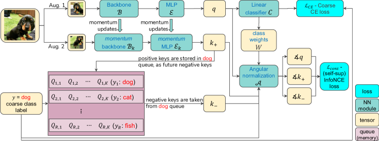
Figure 4: ancor method overview - training flow. For illustrative purposes, showing a single image flow instead of a batch. The query $q$ and the positive key $k_{+}$ are computed from two random augmentations of the input image via the model ($\mathcal{B}\to\mathcal{E}$) and its momentum-updated counterpart ($\mathcal{B}_{k}\to\mathcal{E}_{k}$) [17]. The negative keys $k_{-}$ are taken from the queue $\mathcal{Q}_{y}$ corresponding to the coarse class $y$ of the image. $q$ is classified to the coarse classes by linear classifier $C$, which is followed by the (supervised) CE loss $\mathcal{L}_{CE}$. The (self-supervised) InfoNCE loss $\mathcal{L}_{cont}$ is not applied directly on $q$, $k_{+}$, and $k_{-}$. Doing so would result in disagreement between supervised and self-supervised losses objectives. Instead, $q$, $k_{+}$, and $k_{-}$ are first normalized with the proposed Angular normalization component $\mathcal{A}$ using the linear classifier $C$ weights $W$ corresponding to $y$. This disentangles the forces applied by the two losses, effectively leading to greater synergy between them and consequently to increased performance, as demonstrated by our experiments and ablations.

Coarse and fine learning. Relatively few works have considered learning problems entailing mixing of coarse and fine labels. Several works [43, 15, 52] consider the partially fine-supervised training setting, where during training a mix of (equal #) coarse- and fine- labeled samples is used for training. In contrast, in this work we focus on training using only coarse-labeled data, while fine categories are added at test time and from very few examples (usually one). [20] extends the partially fine-supervised setting to unbalanced splits between coarse- and fine- labeled samples via a MAML-like [10] optimization, albeit in multi-label classification setting (and non-standard performance measure). Similarly, [44] also explores the unbalanced partially fine-supervised setting. Prototype propagation between coarse and fine classes on a known (in advance) class ontology graph is explored in [33] in the few-shot context and in partially fine-supervised training setting, also assuming full knowledge of the classes graph (which also includes the test classes). Finally, a concurrent work of [61] focuses on a scenario similar to C2FS. In [61] the learning is split into three separate consecutive steps: (i) feature learning using a combination of supervised learning with coarse labels and general batch-contrastive learning disregarding classes; (ii) greedy clustering of each coarse class into a set of (fine) pseudo-sub-classes in the resulting feature space; (iii) applying a meta-learning techniques to fine-tune the model to the set of generated pseudo-sub-classes. In contrast, in our ancor approach the model is trained end-to-end, contrastive learning is done within the coarse classes, and we propose a special angular loss component for significantly enhancing the supervised and self-supervised contrastive learning synergies. As a result, in section 4.4.2, we obtain good gains over [61] on the same tieredImageNet test.

3 Method

3.1 Coarse-to-Fine Few-Shot (C2FS) task

Denote by $\mathcal{Y}_{coarse}=\{y_{1},...,y_{R}\}$ a set of $R$ coarse training classes (e.g. kinds of animals: dog, cat, fish, …), and let ${\mathcal{S}_{train}^{coarse}=\{(I_{j},y_{j})|y_{j}\in\mathcal{Y}_{coarse}\}_{j=1}^{N}}$ be a set of $N$ training images annotated (only) with $\mathcal{Y}_{coarse}$. Let ${\mathcal{Y}_{fine}=\{y_{1,1},...,y_{1,k_{1}},y_{2,1},...,y_{2,k_{2}},...,y_{R,1},...y_{R,k_{R}}\}}$ be a set of fine sub-classes (e.g. animal breeds) of the coarse classes $\mathcal{Y}_{coarse}$. In our experiments we also explore the case when fine classes are sub-classes of unseen coarse classes. Let $\mathcal{B}$ be an encoder (CNN backbone) mapping images to a $d$-dimensional feature space $\mathcal{F}\subset\mathbb{R}^{d}$ (i.e. $\mathcal{B}(I_{j})=F_{j}\in\mathcal{F}$) trained on $\mathcal{S}_{train}$. Provided at test time with a small $k$-shot training set for a subset $\mathcal{Y}_{fine}^{m}\subseteq\mathcal{Y}_{fine}$ of $m$ fine classes: $\mathcal{S}_{train}^{fine}=\{(I_{r},y_{r})|y_{r}\in\mathcal{Y}_{fine}^{m}\}_{r=1}^{k\cdot m}$ our goal is to train a classifier $C:\mathcal{F}\to\mathcal{Y}_{fine}^{m}$ with maximal accuracy on the $\mathcal{Y}_{fine}^{m}$ fine classes test set. For example, $m$ could also be $\sum k_{i}$ making $\mathcal{Y}_{fine}^{m}=\mathcal{Y}_{fine}$ (’all-way’). Note that during training of $\mathcal{B}$ the set of fine sub-classes $\mathcal{Y}_{fine}$ is unknown. Also note that according to [58, 55, 31], SOTA few-shot performance can be achieved even without modifying $\mathcal{B}$ when adapting to (unseen) test classes.

3.2 The (ancor) approach

At its core, our method focuses on learning $\mathcal{B}$ combining (with added synergy) supervised learning for inter-class separation of the coarse classes $\mathcal{Y}_{coarse}$ and contrastive self-supervised learning for separating the fine sub-classes within each coarse class ($\mathcal{Y}_{fine}$). The training architecture of ancor is illustrated in Fig. 4. Our model is comprised of: (i) a CNN encoder $\mathcal{B}:I\to\mathbb{R}^{d}$ with Global Average Pooling (GAP) on top (e.g. ResNet50 mapping images to $2048$-dimensional vectors); (ii) an MLP embedder module $\mathcal{E}:\mathbb{R}^{d}\to\mathbb{R}^{e}$ with $e<d$ (e.g. $2048\to 2048\to 128$), $\mathcal{E}$ also includes $L_{2}$ normalization of the final vector; (iii) second pair of (momentum) encoder $\mathcal{B}_{k}$ and (momentum) embedder $\mathcal{E}_{k}$ for encoding the positive keys in the contrastive objective that are momentum updated from $\mathcal{B}$ and $\mathcal{E}$ respectively (following [17]); (iv) a linear classifier $C:\mathbb{R}^{e}\to\mathcal{Y}_{coarse}$ without bias and $W\in\mathbb{R}^{R\times e}$ its weight matrix (so $W\cdot\mathcal{E}(\mathcal{B}(I))$ are the $R$ coarse classes logits of $C$); (v) a set of per-class ’negative-instance’ queues $\{\mathcal{Q}_{i}\}_{i=1}^{R}$, with each queue: $\mathcal{Q}_{i}\in\mathbb{R}^{e\times K}$ of length $K$ (different from [17] that utilized a single queue for the entire dataset); and (vi) an Angular normalization module explained below, that is used for inducing synergy between the supervised and self-supervised contrastive losses by disentangling the forces they apply on samples in the feature space.

The training (Fig. 4) proceeds in batches, but for clarity here we describe the training process for a single training image $I$ annotated with a coarse class label $y\in\mathcal{Y}_{coarse}$. Abusing notation let $y$ also denote the index of the coarse class in $\mathcal{Y}_{coarse}$. We first augment $I$ twice to get $I_{q}$ and $I_{k}$ which are then passed through the corresponding encoders and embedders to retrieve $q=\mathcal{E}(\mathcal{B}(I_{q}))$ and $k_{+}=\mathcal{E}_{k}(\mathcal{B}_{k}(I_{k}))$. We also set $k_{-}=\mathcal{Q}_{y}$ (being ’momentum’ embeddings of previously encountered samples of the same coarse class $y$, at the end of the training cycle $k_{+}$ is also added to $\mathcal{Q}_{y}$). Our two loss functions are: $\mathcal{L}_{CE}(C(q),y)$ being the coarse-supervised softmax Cross Entropy (CE) on $C(q)=W\cdot q$ logits and $1$-hot vector for $y$ coarse class label; and $\mathcal{L}_{cont}(q,k_{+},k_{-})$ being the $y$ class-specific self-supervised contrastive InfoNCE loss applied to query $q$ positive key $k_{+}$ and negative keys $k_{-}$. However, if used naively, $\mathcal{L}_{CE}$ would try to push $q$ towards the other samples of the same class $y$, while at the same time $\mathcal{L}_{cont}$ would try to push it away from them (as $k_{-}$ represents the other samples of the class). This would diminish the synergy between the losses and, as shown in the ablation study 4.5.1, would result in significant performance drop on the the C2FS task.

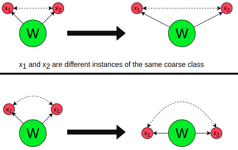
Figure 5: The angular normalization effect. Top: without normalization minimizing the contrastive loss $\mathcal{L}_{cont}$ pushes the samples of the same coarse class $x_{1}$, $x_{2}$ (red) away from each other and thus away from the class weight vector $W$ (green) increasing the supervised loss $\mathcal{L}_{CE}$; Bottom: after angular normalization, $\mathcal{L}_{cont}$ operates on angles in the orbit around the class weight, not affecting the distance between the weight and the samples.

Angular normalization. To improve this synergy, we propose a new module which we name ’angular normalization’. For a given image $I$ with embedding $q$ and coarse label $y$, the logit for class $y$ in classifier $C$ is $W_{y}\cdot q$, where $W_{y}$ is the $y^{th}$ row of $W$. Thus, the supervised loss $\mathcal{L}_{CE}(C(q),y)$ is minimized when $W_{y}\cdot q$ is maximized and $W_{i\neq y}\cdot q$ are minimized, or in other words, when $q$ (unit vector, as the embedder $\mathcal{E}$ ends with $L_{2}$ normalization) shifts towards being in the direction of $W_{y}$. And this is the same for all images of class $y$ essentially encouraging their collapse to $W_{y}/||W_{y}||$ (the unit vector closest to $W_{y}$). But this collapse is in direct conflict of interests with the $y$ class-specific InfoNCE contrastive loss $\mathcal{L}_{cont}(q,k_{+},k_{-})$ that tries to push $y$’s samples away from each other (Fig. 5 top). To solve this, we propose a simple method that can be used to induce synergy between $\mathcal{L}_{CE}$ and $\mathcal{L}_{cont}$. We define the $y$-class specific angular normalizaton:

$$\mathcal{A}(x,W,y)=\angle x=\frac{\frac{x}{\rVert{x}\rVert}-\frac{\mathcal{W}_{y}}{\rVert\mathcal{W}_{y}\rVert}}{\rVert\frac{x}{\rVert{x}\rVert}-\frac{\mathcal{W}_{y}}{\rVert\mathcal{W}_{y}\rVert}\rVert}.$$ (1)

which converts any unit vector $x/||x||$ into a unit vector representing its angle around $W_{y}/||W_{y}||$. With the above definition of angular normalization $\mathcal{A}$, we replace the $q$, $k_{+}$, and $k_{-}$ in $\mathcal{L}_{cont}$ with their $y$-class-specific normalized versions:

$$\angle q =\mathcal{A}(q,W,y)$$ (2)

$$\angle k_{+} =\mathcal{A}(k_{+},W,y)$$ (3)

$$\angle k_{-} =\mathcal{A}(k_{-},W,y)$$ (4)

and obtain our final (full) loss function:

$$\mathcal{L}=\mathcal{L}_{CE}(C(q),y)+\mathcal{L}_{cont}(\angle q,\angle k_{+},\angle k_{-})$$ (5)

where the angular normalized contrastive loss $\mathcal{L}_{cont}(\angle q,\angle k_{+},\angle k_{-})$ operates in the space of angles in the ’orbit’ around $W_{y}/||W_{y}||$, thus not interfering with the ’drive to collapse to $W_{y}/||W_{y}||$’ dictated by the $\mathcal{L}_{CE}$ loss (Fig. 5 bottom). An additional intuitive benefit of the $\mathcal{A}$ normalization is that it ignores the distance to the (normalized) class weight vector, thus protecting $\mathcal{L}_{cont}$ from bias caused by different ’tighter’ or ’looser’ sub-classes.

3.3 Few-shot testing on fine classes

At test time, only the encoder $\mathcal{B}$ followed by $L_{2}$ normalization is retained as the feature extractor and following [6] the MLP embedder $\mathcal{E}$ is dropped (for higher performance). According to our definition of C2FS task, only a small $k$-shot and $m$-way training set $\mathcal{S}_{train}^{fine}$ is available for adapting the model to support the fine-classes. For the few-shot classifier we use the method of [55]. For every few-shot episode, we create 5 augmented copies for every support sample, and train a logistic regression model on the support set encoded using $\mathcal{B}$ followed by $L_{2}$ normalization. The model with the resulting logistic regression classifier on top is then used to classify the query samples of the episode.

4 Experiments

4.1 Datasets

Our experiments were performed on: (i) BREEDS [46], four datasets derived from ImageNet with class hierarchy re-calibrated by [46] so classes on same hierarchy level are of the same visual granularity (not so in the WordNet hierarchy); (ii) CIFAR-100 [25]; and (iii) tieredImageNet [42], a subset of ImageNet, with train/val/test built from different coarse classes. Datasets are summarised in Table 1.

Dataset	L17	NL26	E13	E30	CIFAR100	Tiered
# Coarse classes	17	26	13	30	20	20/6
# Fine classes	68	104	260	240	100	351/160
# Train images	88K	132K	334K	307K	50K	448K
# Test images	3.4K	5.2K	13K	12K	10K	206K
Image resolution	224	224	224	224	32	84

Table 1: Datasets: L17, NL26, E13 & E30 are the Living17, NonLiving17, Entity13 & Entity30 from BREEDS. For Tiered the train/val/test classes are non overlapping; For CIFAR-100 and BREEDS val was 10% of the train, Tiered has pre-defined val set.

	LIVING-17		NONLIVING-26		ENTITY-13		ENTITY-30
Method	5-way	all-way	5-way	all-way	5-way	all-way	5-way	all-way
Fine (upper-bound)	91.10 $\pm$ 0.47	58.95 $\pm$ 0.16	85.25 $\pm$ 0.49	47.68 $\pm$ 0.13	91.01 $\pm$ 0.39	50.19 $\pm$ 0.08	91.65 $\pm$ 0.41	56.54 $\pm$ 0.09
Fine$+$ (upper-bound)	78.39 $\pm$ 0.64	46.92 $\pm$ 0.16	74.95 $\pm$ 0.57	39.57 $\pm$ 0.11	85.98 $\pm$ 0.55	47.87 $\pm$ 0.09	85.43 $\pm$ 0.57	45.87 $\pm$ 0.09
MoCoV2	56.66 $\pm$ 0.70	18.57 $\pm$ 0.11	63.51 $\pm$ 0.75	21.07 $\pm$ 0.11	82.00 $\pm$ 0.67	33.06 $\pm$ 0.07	80.37 $\pm$ 0.62	28.62 $\pm$ 0.06
MoCoV2-ImageNet [5]	82.21 $\pm$ 0.73	40.29 $\pm$ 0.14	77.07 $\pm$ 0.78	34.78 $\pm$ 0.13	85.24 $\pm$ 0.6	35.62 $\pm$ 0.08	83.06 $\pm$ 0.62	31.73 $\pm$ 0.08
SWAV-ImageNet [2]	79.83 $\pm$ 0.65	38.79 $\pm$ 0.15	76.26 $\pm$ 0.71	33.94 $\pm$ 0.11	81.15 $\pm$ 0.65	33.57 $\pm$ 0.07	79.91 $\pm$ 0.54	31.15 $\pm$ 0.07
Coarse	85.12 $\pm$ 0.74	33.83 $\pm$ 0.10	83.53 $\pm$ 0.64	33.52 $\pm$ 0.11	82.33 $\pm$ 0.61	17.49 $\pm$ 0.04	87.03 $\pm$ 0.54	24.01 $\pm$ 0.06
Coarse$+$	79.29 $\pm$ 0.65	37.44 $\pm$ 0.12	75.91 $\pm$ 0.66	36.80 $\pm$ 0.11	83.23 $\pm$ 0.66	31.15 $\pm$ 0.07	84.81 $\pm$ 0.61	33.22 $\pm$ 0.08
ancor (ours)	89.23 $\pm$ 0.55	45.14 $\pm$ 0.12	86.23 $\pm$ 0.54	43.10 $\pm$ 0.11	90.58 $\pm$ 0.54	42.29 $\pm$ 0.08	88.12 $\pm$ 0.54	41.79 $\pm$ 0.08

Table 2: Results for different baselines on the four BREEDS datasets. Top section contains models trained with fine-grained labels that serve as upper bounds, middle section contains baselines, and the bottom section is our results.

4.2 Baselines

As C2FS task is new, we propose a diverse set of natural baselines and upper bounds for the task. We also compare to the concurrent work of [61] where applicable. For fair comparison, we use $200$ train epochs for all models (ours, baselines). The effect of longer training is explored in section 4.5.5. Hyper-parameters of all compared methods were tuned on val sets. For the baselines and upper bounds we also used the best training practices from [55], including self-distillation, which consistently improved their performance. For fairness, in each experiment all compared methods use the same backbone architecture (for the encoder $\mathcal{B}$).

Coarse Baselines: models trained using coarse labels and with $\mathcal{L}_{CE}$ loss. We consider two such models: (i) ’Coarse’ being the encoder $\mathcal{B}$ followed by a linear classifier $C$; (ii) ’Coarse$+$’ being $\mathcal{B}\to\mathcal{E}\to C$ which has the same number of learned parameters as our ancor model. At test time, the MLP embedder $\mathcal{E}$ is dropped from Coarse$+$ for higher performance (same as for ancor ).

Self-supervised Baselines: Two baselines of MoCoV2 [5]: (i) ’MocoV2’ is using the [5] official code to train on respective training sets; (ii) ’MocoV2-ImageNet’ is the official full ImageNet pre-trained model of [5]. Similarly, ’SWAV-ImageNet’ is the official model of [2]. Note that full ImageNet pre-trained models saw more data during training than did ancor , and yet, interestingly, ancor attains better results. Finally, ’naive combination’ of supervised and self-supervised losses without our angular normalization $\mathcal{A}$ is explored in ablation (Sec. 4.5.1). Due to lack of space, additional baselines are provided in Supplementary.

Fine Upper-Bound: a natural performance upper-bounds for ancor are the $\mathcal{B}\to C$ and $\mathcal{B}\to\mathcal{E}\to C$ models trained on the fine labels of the respective training sets (hidden from ancor according to the C2FS task definition). To be consistent with the coarse baselines naming convention, we call them ’Fine’ and ’Fine$+$’ respectively. To match the evaluation setting, for both ’Fine’ and ’Fine$+$’ we also drop the classifier $C$ and embedder $\mathcal{E}$ when few-shot testing.

4.3 Additional implementation details

The encoder $\mathcal{B}$ was: ResNet-50 [18] for the $224\times 224$ datasets (BREEDS [46]), and ResNet-12 for the small resolution datasets (CIFAR-100 [25] and tieredImageNet [42]), as is common in the self-supervised and few-shot works respectively. The output dim of these networks is $d=2048$ or $d=640$, respectively. Our MLP embedder $\mathcal{E}$ consisted of two stacked fully connected layers with ReLu activation: $d\to d\to e$, we used $e=128$ in all experiments. We used cosine-annealing with warm restarts schedule [34] with 20 epochs per cycle. We trained on 4 V100 GPUs, with a batch size $b=256$ and base learning rate $lr=0.03$ for BREEDS, and $b=1024$ and $lr=0.12$ for CIFAR-100 and tieredImageNet. We used $wd=1e^{-4}$ weight decay. We used queue size $K=65536$, InfoNCE temperature of $\tau=0.2$, and $m=0.999$ for the momentum encoder ($m=0.99$ for CIFAR-100). All hyper-parameters were optimized on val sets, using the same optimization for our method and the baselines. Code: github.com/guybuk/ANCOR.

4.4 Results

We report results for 5-way $k$-shot and all-way $k$-shot $15$-query tests. Following [55] we evaluate on 1000 random episodes and report the mean accuracy and the 95% confidence interval. Unless explicitly stated $k=1$. Effect of more shots is evaluated in section 4.5.2. The test classes of each episode are a random subset of the set of fine classes $\mathcal{Y}_{fine}$ (or all of them in all-way tests). In section 4.5.3, in order to further investigate the sources of our improvements, we evaluate a special case of ’intra-class’ testing, when all the categories of the episode belong to the same (randomly sampled) coarse class.

4.4.1 Unseen fine sub-classes of seen coarse classes

We first evaluate the core use-case of the C2FS task, namely training on coarse classes $\mathcal{Y}_{coarse}$ and generalizing to fine sub-classes of those classes $\mathcal{Y}_{fine}$ as defined in section 3.1. We used BREEDS and CIFAR-100 for this evaluation, and the results are reported in Tables 2 and 3 respectively. As can be seen, ancor significantly outperforms the coarse baselines across all datasets, in both the 5-way and the all-way tests (e.g. on BREEDS, by over 10% on 5-way and over 5% on all-way). Notably, in NONLIVING-26 5-way, our model surpasses even the Fine models. Moreover, on BREEDS we observe large gains (over 5% in 5-way and over 6% in all-way) over full ImageNet pre-trained self-supervised baselines in all datasets. This suggests that even significantly larger and more diverse training data available to those models is not sufficient to bridge the gap of coarse classes supervision which is needed for the C2FS, and is effectively utilized by ancor in good synergy with the self-supervised objective (due to our angular component). In the supplementary we explore a ’sub-population shift’ variant of this scenario where the sub-classes appearing in training (with the coarse class label only) are non-overlapping with those appearing in the test.

	5-way	all-way
Fine (upper-bound)	74.36 $\pm$ 0.68	28.82 $\pm$ 0.11
Fine$+$ (upper-bound)	69.65 $\pm$ 0.67	27.00 $\pm$ 0.11
MoCo V2	48.07 $\pm$ 0.68	10.61 $\pm$ 0.06
Coarse	74.40 $\pm$ 0.70	27.37 $\pm$ 0.11
Coarse$+$	70.69 $\pm$ 0.69	26.16 $\pm$ 0.10
ancor (ours)	74.56 $\pm$ 0.70	29.84 $\pm$ 0.11

Table 3: Results on CIFAR-100.

4.4.2 Unseen fine sub-classes of unseen coarse classes

We use the tieredImageNet dataset to evaluate the second use-case for C2FS task: when the fine classes $\mathcal{Y}_{fine}$ are not sub-classes of the training coarse classes $\mathcal{Y}_{coarse}$, and in fact belong to a different branch of the classes taxonomy, and yet $\mathcal{Y}_{fine}$ are of significantly higher visual granularity then $\mathcal{Y}_{coarse}$. We train using only the coarse labels of tieredImageNet train classes, and evaluate on its standard test set (with its fine labels). As tieredImageNet is a standard few-shot benchmark, here we compare to the few-shot SOTA methods [55, 19, 62] trained using coarse train labels. The results of this experiment are summarized in Table 4 showing significant advantage of ancor over the baselines. Interestingly, the self-supervised MoCoV2 lags (significantly) behind, underlining the benfit of additional coarse supervision even in situation when test classes are descendants of different coarse classes. Notably, ancor also has a good 3%-5% advantage over the results of the concurrent work of [61] also dealing with coarse-and-fine few-shot interplay and performing the same experiment.

	5-way	5-way	All-way
	1-shot	5-shot	1-shot
[55] fine (upper-bound)	70.15 $\pm$ 0.70	84.96 $\pm$ 0.47	15.42 $\pm$ 0.06
[55] coarse	61.61 $\pm$ 0.74	75.72 $\pm$ 0.56	8.42 $\pm$ 0.04
MoCoV2	53.19 $\pm$ 0.68	70.90 $\pm$ 0.58	8.33 $\pm$ 0.04
CAN [19]	56.91 $\pm$ 0.55	69.76 $\pm$ 0.46	6.29 $\pm$ 0.08
BDE-MetaBL [61]	60.54 $\pm$ 0.79	75.22 $\pm$ 0.63	N/A
DeepEMD [62]	62.84 $\pm$ 0.71	76.95 $\pm$ 0.76	9.65 $\pm$ 0.15
ancor (ours)	63.54 $\pm$ 0.70	80.12 $\pm$ 0.53	11.97 $\pm$ 0.06

Table 4: Results on tieredImageNet.

4.5 Analysis

We used the LIVING-17 dataset for the analysis.

4.5.1 Ablation study

Here we evaluate several design choices of the ancor approach. In terms of architecture, we compare two variants of the coarse-supervised branch: (i) ’Seq’ being $\mathcal{B}\to\mathcal{E}\to C\to\mathcal{L}_{CE}$; and (ii) ’Fork’ being $\mathcal{B}\to\mathcal{E}_{layer\#1}\to C\to\mathcal{L}_{CE}$. In both cases the self-supervised contrastive branch remains the same: $\mathcal{B}\to\mathcal{E}\to\mathcal{L}_{cont}$. We also test the contribution of the angular normalization $\mathcal{A}$ in the self-supervised branch (between $\mathcal{E}$ and $\mathcal{L}_{cont}$). Of Seq and Fork, only Seq admits the possibility for angular normalization, as in Fork the classifier weights are of different dimensionality ($\text{dim}=d$) than the output of $\mathcal{E}$ ($\text{dim}=e$). Finally, we also evaluate the contribution of having a queue $\mathcal{Q}_{i}$ for each class (’Multi’) vs. simply stacking all negative keys in a single shared queue $\mathcal{Q}$ (’Single’). The results of this ablation are presented in Table 5. Looking at all-way results we draw the following conclusions: (i) difference between Seq and Fork is small; (ii) without angular normalization single queue is better than multi-queue in all-way, likely because $\mathcal{L}_{cont}$ negative keys $k_{-}$ taken from the shared queue do not belong to the same class (as opposed to Multi with queue per class) reducing the $\mathcal{L}_{cont}$ drive to disperse same class elements in feature space; (iii) angular normalization gives a significant boost both to Single+Seq and to Multi+Seq; and (iv) Multi+Seq is best when combined with angular normalization forming ancor.

	MQ	S/F	$\mathcal{A}$	5-way	all-way
Single+Fork	✗	F	✗	82.45	42.75
Multi+Fork	✓	F	✗	85.38	36.28
Single+Seq	✗	S	✗	79.44	41.55
Multi+Seq	✓	S	✗	81.75	36.06
Single+Seq+Angular	✗	S	✓	82.1	42.62
ancor (ours) Multi+Seq+Angular	✓	S	✓	89.23	45.14

Table 5: Architecture ablations. (1) MQ: Multi queue (queue per class, otherwise one queue for all classes [17]) (2) S/F: Sequential or Fork architecture. (3) $\mathcal{A}$: Angular normalization component.

4.5.2 The effect of adding more shots

Here we evaluate the effect of adding more shots (number of support samples per class) to the few-shot episodes during testing. The results are shown in Fig. 6 demonstrating ancor’s consistent advantage (of about $+5\%$ accuracy in all-way) above the strongest of self-supervised (MocoV2-ImageNet) and supervised (Coarse+) baselines.

	all-way	intra-class	all-way
	(coarse)	(fine)	(fine)
Coarse	81.44 $\pm$ 0.31	37.03 $\pm$ 0.53	33.83 $\pm$ 0.1
Coarse$+$	50.83 $\pm$ 0.32	46.56 $\pm$ 0.65	37.44 $\pm$ 0.12
MoCoV2	27.36 $\pm$ 0.23	47.7 $\pm$ 0.62	18.57 $\pm$ 0.11
ancor (ours)	84.25 $\pm$ 0.31	48.77 $\pm$ 0.71	45.14 $\pm$ 0.12

Table 6: Closer look on all-way (fine test labels) result breaking it into all-way with coarse test labels and intra-class-fine (fine classes of same random coarse class).

4.5.3 Closer look at the fine classes performance

Success in C2FS entails both not confusing the coarse classes as well as not confusing the fine sub-classes of each class. Therefore we ask ourselves, is the benefit of ancor coming from less coarse confusion or from less (intra-class) fine confusion? Looking at Table 6 we see that ancor has better all-way coarse accuracy (using coarse-only labels of the test set), as well as better intra-class fine accuracy evaluated by creating the few-shot episodes by random sampling a coarse class $y_{i}\in\mathcal{Y}_{coarse}$ and then generating a random episode from (all of) it’s sub-classes $\{y_{i,1},...,y_{i,k_{i}}\}$. Consequently, ancor has the highest performance on the all-way fine test that we also saw in Tab. 2. Interestingly, Coarse, Coarse$+$, and MoCoV2 results indicate there is a trade-off between all-way coarse and intra-class-fine performances, trade-off apparently topped by ancor.

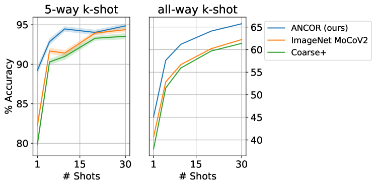
Figure 6: 5-way and all-way results with increasing $k$ shots.

4.5.4 Closer look at the features

We further explore the feature space $\mathcal{F}$ learned by ancor using visualizations. Fig. 2 visualizes $\mathcal{F}$ on ENTITY-13 via tSNE and compares it to the tSNE plots of the feature space of the Coarse baseline, both on the coarse classes level and when digging into a random coarse class, qualitatively showing an advantage for ancor ’s feature space. In addition, in figure 7 we show a simple heatmap visualization of activations of the last convolutional layer of $\mathcal{B}$ obtained by dropping the GAP at the end of $\mathcal{B}$ and for each feature vector $f$ corresponding to a spatial coordinate in the resulting tensor computing the norm of the activation $||\mathcal{E}(f)||^{2}$. To obtain a higher resolution for this visualization we also increase the input image resolution by $\times 2$. Surprisingly, despite the relatively small number of coarse classes (not benefiting spatial specificity), and the instance recognition nature of the self supervised objective (that could in principle use background pixels to discriminate instance images), the features learned by ancor trained $\mathcal{B}$ are remarkably good at localizing the object instances essentially ignoring the background. We verified this phenomena is stable and repeating in almost all localizations we examined and would be very interesting to explore in future studies.

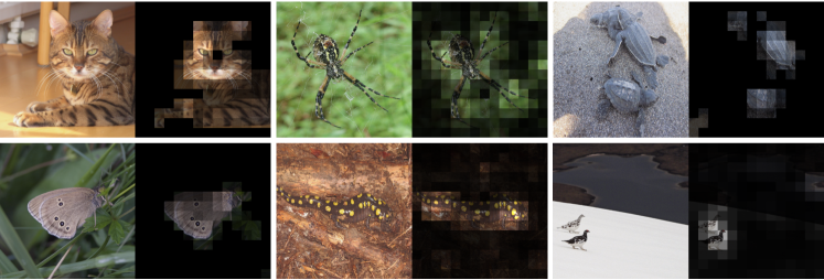
Figure 7: ancor encoder $\mathcal{B}$ last layer activations examples.

4.5.5 Longer training

In all above experiments, for fair comparison we used 200 epochs for training all models (ancor, baselines and upper bounds). In Fig. 8 we explore what happens if we train longer. As can be seen, there is still much to be gained from ancor with longer training. We attribute this positive effect to the contrastive component that is known to benefit from longer training [2, 5]. Almost 15% gains are observed for ancor when increasing the number of epochs from 200 to 800, and interestingly, ancor ’s ’all-way’ gain above the baselines becomes larger with more epochs.

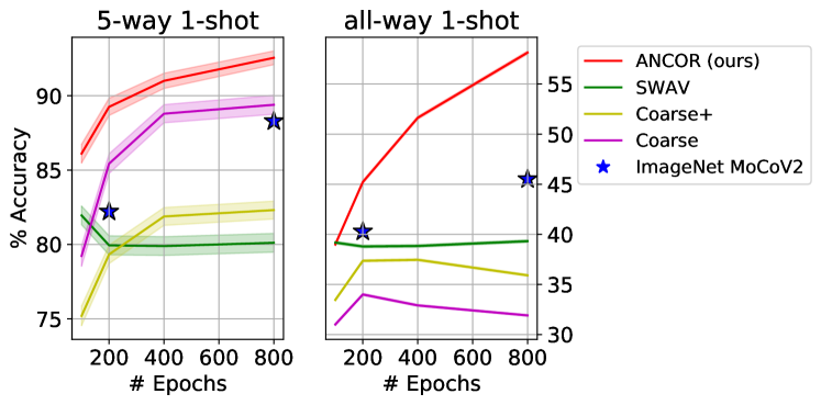
Figure 8: Results for 5-way and all-way tests, reporting with an increasing number of epochs.

5 Summary and conclusions

We have proposed the C2FS task focusing on situations when a few-shot model needs to adapt to much finer-grained unseen classes than the base classes used during its pre-training, including the challenging case when the unseen target classes are sub-classes of the base classes. We introduced the ancor approach for the C2FS task based on effective combination of inter-class supervised and intra-class self-supervised losses featuring a novel ’angular normalization’ component inducing synergy between these (otherwise conflicting) losses. We have demonstrated the effectiveness of ancor on a variety of datasets showing: (i) promising results of ancor on the C2FS task also in the more challenging ’all-way’ setting; (ii) that the proposed angular component is instrumental in the success of ancor; (iii) the advantages of ancor are preserved when adding more shots for the fine classes; (iv) ancor does best also in the challenging ’intra-class fine’ scenario when all target classes belong to the same coarse class; (v) promising properties of ancor feature space including surprisingly good spatial attention to object instances; and (vi) ancor can be improved considerably with longer training, getting larger improvements on C2FS task than even leading self-supervised methods trained on more data ([5, 2]). We hope that this work will serve as a good basis for future research into the exciting and challenging C2FS task further pushing its limits. Finally, we believe that the proposed angular normalization component is useful beyond the C2FS task for any situation involving supervised and contrastive self-supervised multi-tasking, and leave it to future works to explore its uses further.

6 Appendix

6.1 Additional baselines

	LIVING-17		NONLIVING-26		ENTITY-13		ENTITY-30
Method	5-way	all-way	5-way	all-way	5-way	all-way	5-way	all-way
ensemble(Coarse+, MoCoV2)	74.07 $\pm$ 0.67	34.02 $\pm$ 0.13	73.14 $\pm$ 0.71	33.23 $\pm$ 0.11	85.27 $\pm$ 0.57	36.39 $\pm$ 0.08	84.22 $\pm$ 0.6	34.56 $\pm$ 0.08
ensemble(Coarse, MoCoV2)	84.32 $\pm$ 0.62	36.39 $\pm$ 0.13	79.95 $\pm$ 0.65	34.31 $\pm$ 0.11	85.97 $\pm$ 0.59	34.03 $\pm$ 0.08	88.48 $\pm$ 0.55	34.49 $\pm$ 0.08
cascade(Coarse+,MoCoV2)	74.1 $\pm$ 0.66	34.04 $\pm$ 0.13	73.1 $\pm$ 0.7	33.23 $\pm$ 0.11	85.19 $\pm$ 0.57	36.38 $\pm$ 0.08	84.33 $\pm$ 0.6	34.57 $\pm$ 0.08
cascade(Coarse,MoCoV2)	88.27 $\pm$ 0.63	38.02 $\pm$ 0.14	84.66 $\pm$ 0.64	36.05 $\pm$ 0.11	86.39 $\pm$ 0.59	35.46 $\pm$ 0.07	90.02 $\pm$ 0.55	37.1 $\pm$ 0.08
concat(Coarse+,MoCoV2)	73.48 $\pm$ 0.66	33.4 $\pm$ 0.13	71.49 $\pm$ 0.71	31.28 $\pm$ 0.11	84.26 $\pm$ 0.59	35.64 $\pm$ 0.08	83.03 $\pm$ 0.62	33.5 $\pm$ 0.07
concat(Coarse,MoCoV2)	83.45 $\pm$ 0.63	35.89 $\pm$ 0.13	77.59 $\pm$ 0.67	32.48 $\pm$ 0.11	85.35 $\pm$ 0.6	33.89 $\pm$ 0.07	86.83 $\pm$ 0.57	33.82 $\pm$ 0.07
Supervised Contrastive [23]	86.49 $\pm$ 0.67	35.11 $\pm$ 0.12	84.54 $\pm$ 0.61	37.44 $\pm$ 0.11	87.08 $\pm$ 0.58	28.57 $\pm$ 0.15	88.86 $\pm$ 0.52	33.67 $\pm$ 0.17
ancor (ours)	89.23 $\pm$ 0.55	45.14 $\pm$ 0.12	86.23 $\pm$ 0.54	43.10 $\pm$ 0.11	90.58 $\pm$ 0.54	42.29 $\pm$ 0.08	88.12 $\pm$ 0.54	41.79 $\pm$ 0.08

Table 7: Additional baselines: evaluated using BREEDS [46] with $1$-shot. The ”Coarse”, ”Coarse+”, and ”MoCoV2” models used in ensemble and cascade combinations are as described in the paper. (1) ensemble: averaging the two models predictions (probabilities after softmax); (2) cascade: classify into the max-scoring coarse classes $\mathcal{Y}_{coarse}$ using the coarse-supervised model (with the linear classifier resulting from pre-training), and then use the self-supervised model (with the LR classifier, paper Sec. 3.3) for intra-class classification within the chosen coarse class (limiting the target classes to its sub-classes); (3) concat: concatenate the feature vectors from the two models and then apply few-shot classification as in the paper Sec. 3.3; (4) Same as Coarse+ using the Supervised Contrastive loss [23] replacing CE.

	Good	Bad	5-way	all-way
Coarse$+$		✓	70.77 $\pm$ 0.74	36.65 $\pm$ 0.19
Coarse$+$	✓		73.44 $\pm$ 0.69	43.13 $\pm$ 0.22
ancor (ours)		✓	74.99 $\pm$ 0.71	40.69 $\pm$ 0.20
ancor (ours)	✓		77.32 $\pm$ 0.69	47.53 $\pm$ 0.22

Table 8: Sub-population Shift. Two hand-crafted partitions of the LIVING-17 dataset, created by [46], such that the test sub-classes are different from the (unlabeled) training sub-classes, yet share the common coarse classes. ’Good’ and ’Bad’ represent a less and more adversarial partitioning. Note that in practice these models train on half the data the models trained on LIVING-17 in the main paper have, due to the partitioning.

We include $7$ additional baseline comparisons using the four BREEDS [46] datasets. These baselines were not included in the main paper due to lack of space. The comparisons are summarized in Table 7. We include several kinds of additional baselines covering different possible supervised + self-supervised combinations, as well as of supervised contrastive loss use:

• ensemble (of Coarse/Coarse+ with MoCoV2): averaging the two models predictions (probabilities after softmax)

• cascade (of Coarse/Coarse+ with MoCoV2): classify into the max-scoring coarse classes $\mathcal{Y}_{coarse}$ using the coarse-supervised model (with the linear classifier resulting from pre-training), and then use the self-supervised model (with the LR classifier, Section 3.3 in the paper) for intra-class classification within the chosen coarse class (limiting the target classes to the sub-classes of the predicted coarse class)

• concat (of Coarse/Coarse+ with MoCoV2): concatenating the features produces by the two models, and doing few-shot classification via learning the logistic regression (paper Section 3.3) on the resulting concatenated features.

• Supervised Contrastive: Training with coarse labels $\mathcal{Y}_{coarse}$ using the Supervised Contrastive loss [23] replacing CE.

The ”Coarse”, ”Coarse+”, and ”MoCoV2” models used in ensemble, cascade, and concat combinations are as described in the paper. As can be seen from the table, in all (the more challenging) all-way experiments ancor maintains a significant advantage over the baselines, even ones combining (via an ensemble, a cascade, or a concat) separately trained coarse-supervised and contrastive self-supervised models, and thus also using twice more learn-able parameters than ancor. This demonstrates once again the importance of joint coarse-supervised and contrastive self-supervised training employed by ancor and facilitated by the proposed angular normalization component enhancing the synergy between these two objectives.

	LIVING-17		NONLIVING-26		ENTITY-13		ENTITY-30
Method	5-way	all-way	5-way	all-way	5-way	all-way	5-way	all-way
Fine (upper-bound)	91.94 $\pm$ 0.44	64.66 $\pm$ 0.17	87.68 $\pm$ 0.50	54.42 $\pm$ 0.13	94.22 $\pm$ 0.34	64.30 $\pm$ 0.09	93.11 $\pm$ 0.38	61.70 $\pm$ 0.09
Fine$+$ (upper-bound)	90.25 $\pm$ 0.48	63.54 $\pm$ 0.17	86.27 $\pm$ 0.51	53.16 $\pm$ 0.14	91.99 $\pm$ 0.40	59.43 $\pm$ 0.09	91.03 $\pm$ 0.43	57.48 $\pm$ 0.09
MoCoV2	81.45 $\pm$ 0.61	46.65 $\pm$ 0.16	78.33 $\pm$ 0.65	42.08 $\pm$ 0.12	87.30 $\pm$ 0.53	48.97 $\pm$ 0.08	86.51 $\pm$ 0.56	46.77 $\pm$ 0.09
MoCoV2-ImageNet [5]	89.27 $\pm$ 0.57	51.60 $\pm$ 0.15	82.22 $\pm$ 0.66	43.32 $\pm$ 0.12	88.30 $\pm$ 0.55	45.52 $\pm$ 0.08	87.18 $\pm$ 0.58	42.23 $\pm$ 0.08
SWAV-ImageNet [2]	80.11 $\pm$ 0.63	39.30 $\pm$ 0.14	73.43 $\pm$ 0.67	33.06 $\pm$ 0.11	79.58 $\pm$ 0.62	33.36 $\pm$ 0.07	78.89 $\pm$ 0.64	31.16 $\pm$ 0.07
Coarse	89.04 $\pm$ 0.63	29.06 $\pm$ 0.23	84.72 $\pm$ 0.63	27.99 $\pm$ 0.18	82.66 $\pm$ 0.75	11.24 $\pm$ 0.08	90.09 $\pm$ 0.59	20.63 $\pm$ 0.12
Coarse$+$	89.41 $\pm$ 0.61	33.07 $\pm$ 0.23	84.69 $\pm$ 0.59	32.07 $\pm$ 0.20	85.23 $\pm$ 0.63	22.85 $\pm$ 0.13	88.43 $\pm$ 0.55	28.33 $\pm$ 0.15
ancor (ours)	92.59 $\pm$ 0.47	58.15 $\pm$ 0.16	88.25 $\pm$ 0.52	49.38 $\pm$ 0.13	92.04 $\pm$ 0.44	50.72 $\pm$ 0.09	92.13 $\pm$ 0.44	50.85 $\pm$ 0.09

Table 9: Results for different baselines on the four BREEDS datasets. Every model was trained for 800 epochs.

6.2 Sub-population Shift

The ’sub-population shift’ benchmark was proposed in [46] intended to evaluate how classification performance is affected when the train classes and test classes consist of different (non-overlapping set of) sub-classes (eg. ‘Dog‘ class in training consist of samples of ’Bloodhound’ and ’Pekinese’, while the test dogs are the ’Great Pyrenese’ and the ’papillon’). For this purpose they propose two hand-crafted partitions for each of their datasets: named ’good’ and ’bad’, which represent a less and a more adversarial partitioning respectively. We leverage this to create a task that is on one hand allows having the same coarse classes in training and in testing (as in the task in Section 4.4.1), while still having the sub-classes of those coarse classes non-overlapping (different) between the train and the test (as in the task in Section in 4.4.2). In other words, in this scenario the test sub-classes are completely different from the training ones, and yet they share the same parent coarse classes. Our evaluation on this task, provided in Table 8, shows that despite this challenging setting, ancor significantly outperforms the strongest baseline by $>4\%$ in the all-way test.

6.3 Additional results for 800-epoch training

In this section we further examine the effect of longer training longer on the performance. As can be seen in Table 9, following longer 800 epoch training ancor obtains significant gains in all the experimental settings. The most noticeable gains are in the all-way tests, where we observe that the gap above the baselines grows with longer training. We attribute this improvement to the contrastive component that is known to benefit from longer training [2, 5]. Interestingly, with longer training the coarse baseline models have gained accuracy in the 5-way test, but lost accuracy in the all-way test (compared to the 200 epochs performance). This supports our hypothesis that the coarse-classes supervised objective encourages reducing intra-class variation, and as such, with the longer training, tends to decresae the distinction between fine-sub classes loosing their discriminability within the coarse class. This again underlines the merits of our ancor approach that retains and enhances the fine sub-classes discrimnability thus significantly benefiting from the longer training regime.

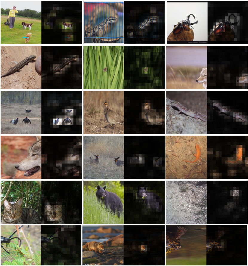
Figure 9: Additional examples of ancor encoder $\mathcal{B}$ last layer activations.

6.4 Additional examples of ancor encoder $\mathcal{B}$ last layer activations

Additional examples of ancor encoder $\mathcal{B}$ last layer activations are provided in Figure 9, again illustrating an interesting attention to objects learned by ancor despite not being provided with any location supervision during training.

Acknowledgments This material is based upon work supported by the Defense Advanced Research Projects Agency (DARPA) under Contract No. FA8750-19-C-1001. Any opinions, findings and conclusions or recommendations expressed in this material are those of the author(s) and do not necessarily reflect the views of DARPA. Raja Giryes was supported by ERC-StG grant no. 757497 (SPADE).

References

- [1] Antreas Antoniou and Amos Storkey. Assume, Augment and Learn: Unsupervised Few-Shot Meta-Learning via Random Labels and Data Augmentation. Technical report.
- [2] Mathilde Caron, Ishan Misra, Julien Mairal, Priya Goyal, Piotr Bojanowski, and Armand Joulin. Unsupervised Learning of Visual Features by Contrasting Cluster Assignments. 6 2020.
- [3] Ting Chen, Simon Kornblith, Mohammad Norouzi, and Geoffrey Hinton. A Simple Framework for Contrastive Learning of Visual Representations. ICML, 2 2020.
- [4] Wei-Yu Chen, Yen-Cheng Liu, Zsolt Kira, Yu-Chiang Wang, and Jia-Bin Huang. A Closer Look At Few-Shot Classification. In ICLR, 2019.
- [5] Xinlei Chen, Haoqi Fan, Ross Girshick, and Kaiming He. Improved Baselines with Momentum Contrastive Learning. arXiv, 3 2020.
- [6] Xinlei Chen, Haoqi Fan, Ross Girshick, and Kaiming He. Improved Baselines with Momentum Contrastive Learning. arXiv, 3 2020.
- [7] Carl Doersch, Abhinav Gupta, and Alexei A Efros. Unsupervised Visual Representation Learning by Context Prediction. In ICCV, 2015.
- [8] Sivan Doveh, Eli Schwartz, Chao Xue, Rogerio Feris, Alex Bronstein, Raja Giryes, and Leonid Karlinsky. MetAdapt: Meta-Learned Task-Adaptive Architecture for Few-Shot Classification. Technical report, 2019.
- [9] Nikita Dvornik, Cordelia Schmid, and Julien Mairal. Diversity with Cooperation: Ensemble Methods for Few-Shot Classification. In ICCV, 2019.
- [10] Chelsea Finn, Pieter Abbeel, and Sergey Levine. Model-Agnostic Meta-Learning for Fast Adaptation of Deep Networks. In ICML, 2017.
- [11] Spyros Gidaris, Andrei Bursuc, Nikos Komodakis, Patrick Pérez, and Matthieu Cord. Boosting Few-Shot Visual Learning with Self-Supervision. In ICCV, 6 2019.
- [12] Spyros Gidaris, Praveer Singh, and Nikos Komodakis. Unsupervised Representation Learning by Predicting Image Rotations. In ICLR. arXiv, 3 2018.
- [13] Jean-Bastien Grill, Florian Strub, Florent Altché, Corentin Tallec, Pierre H. Richemond, Elena Buchatskaya, Carl Doersch, Bernardo Avila Pires, Zhaohan Daniel Guo, Mohammad Gheshlaghi Azar, Bilal Piot, Koray Kavukcuoglu, Rémi Munos, and Michal Valko. Bootstrap your own latent: A new approach to self-supervised Learning. 6 2020.
- [14] Yunhui Guo, Noel C. Codella, Leonid Karlinsky, James V. Codella, John R. Smith, Kate Saenko, Tajana Rosing, and Rogerio Feris. A Broader Study of Cross-Domain Few-Shot Learning. In ECCV, 12 2020.
- [15] Yanming Guo, Yu Liu, Erwin M. Bakker, Yuanhao Guo, and Michael S. Lew. CNN-RNN: a large-scale hierarchical image classification framework. Multimedia Tools and Applications, 77(8):10251–10271, 4 2018.
- [16] Fusheng Hao, Fengxiang He, Jun Cheng, Lei Wang, Jianzhong Cao, and Dacheng Tao. Collect and Select : Semantic Alignment Metric Learning for Few-Shot Learning. ICCV, pages 8460–8469, 2019.
- [17] Kaiming He, Haoqi Fan, Yuxin Wu, Saining Xie, and Ross Girshick. Momentum Contrast for Unsupervised Visual Representation Learning. CVPR, pages 9726–9735, 11 2020.
- [18] Kaiming He, Xiangyu Zhang, Shaoqing Ren, and Jian Sun. Deep Residual Learning for Image Recognition. arXiv:1512.03385, 2015.
- [19] Ruibing Hou, Hong Chang, Bingpeng Ma, Shiguang Shan, and Xilin Chen. Cross Attention Network for Few-shot Classification. NeurIPS, 10 2019.
- [20] Cheng-Yu Hsieh, Miao Xu, Gang Niu, Hsuan-Tien Lin, and Masashi Sugiyama. A PSEUDO-LABEL METHOD FOR COARSE-TO-FINE MULTI-LABEL LEARNING WITH LIMITED SUPERVISION. Technical report.
- [21] Kyle Hsu, Sergey Levine, and Chelsea Finn. Unsupervised Learning via Meta-Learning. ICLR, 10 2019.
- [22] Guoliang Kang, Lu Jiang, Yi Yang, and Alexander G Hauptmann. Contrastive Adaptation Network for Unsupervised Domain Adaptation. Proceedings of the IEEE Computer Society Conference on Computer Vision and Pattern Recognition, 2019-June:4888–4897, 1 2019.
- [23] Prannay Khosla, Piotr Teterwak, Chen Wang, Aaron Sarna, Yonglong Tian, Phillip Isola, Aaron Maschinot, Ce Liu, and Dilip Krishnan. Supervised Contrastive Learning. arXiv, 4 2020.
- [24] Jongmin Kim, Taesup Kim, Sungwoong Kim, and Chang D Yoo. Edge-Labeling Graph Neural Network for Few-shot Learning. In CVPR, 2019.
- [25] Alex Krizhevsky. Learning Multiple Layers of Features from Tiny Images. Technical report. Science Department, University of Toronto, Tech., pages 1–60, 2009.
- [26] Alex Krizhevsky, Ilya Sutskever, and Geoffrey E Hinton. ImageNet Classification with Deep Convolutional Neural Networks. Advances In Neural Information Processing Systems, pages 1–9, 2012.
- [27] Kwonjoon Lee, Subhransu Maji, Avinash Ravichandran, and Stefano Soatto. Meta-Learning with Differentiable Convex Optimization. In CVPR, 2019.
- [28] Hongyang Li, David Eigen, Samuel Dodge, Matthew Zeiler, and Xiaogang Wang. Finding Task-Relevant Features for Few-Shot Learning by Category Traversal. 1, 2019.
- [29] Xinzhe Li, Qianru Sun, Yaoyao Liu, Shibao Zheng, Qin Zhou, Tat-Seng Chua, and Bernt Schiele. Learning to Self-Train for Semi-Supervised Few-Shot Classification. In NeurIPS, pages 1–14, 2019.
- [30] Zhenguo Li, Fengwei Zhou, Fei Chen, and Hang Li. Meta-SGD: Learning to Learn Quickly for Few-Shot Learning. In arXiv:1707.09835, 2017.
- [31] Moshe Lichtenstein, Prasanna Sattigeri, Rogerio Feris, Raja Giryes, and Leonid Karlinsky. TAFSSL: Task-Adaptive Feature Sub-Space Learning for Few-Shot Classification. In ECCV. Springer, Cham, 8 2020.
- [32] Yann Lifchitz, Yannis Avrithis, Sylvaine Picard, and Andrei Bursuc. Dense Classification and Implanting for Few-Shot Learning. In CVPR, 2019.
- [33] Lu Liu, Tianyi Zhou, Guodong Long, Jing Jiang, Lina Yao, and Chengqi Zhang. Prototype Propagation Networks (PPN) for Weakly-supervised Few-shot Learning on Category Graph. Technical report, 2019.
- [34] Ilya Loshchilov and Frank Hutter. SGDR: Stochastic Gradient Descent with Warm Restarts. 5th International Conference on Learning Representations, ICLR 2017 - Conference Track Proceedings, 8 2016.
- [35] Tsendsuren Munkhdalai and Hong Yu. Meta Networks. In Proceedings of machine learning research, page 2554, 2017.
- [36] Mehdi Noroozi and Paolo Favaro. Unsupervised learning of visual representations by solving jigsaw puzzles. In ECCV, volume 9910 LNCS, pages 69–84. Springer Verlag, 3 2016.
- [37] Boris N. Oreshkin, Pau Rodriguez, and Alexandre Lacoste. TADAM: Task dependent adaptive metric for improved few-shot learning. NeurIPS, 5 2018.
- [38] Deepak Pathak, Philipp Krahenbuhl, Jeff Donahue, Trevor Darrell, and Alexei A. Efros. Context Encoders: Feature Learning by Inpainting. In CVPR, volume 2016-December, pages 2536–2544. IEEE Computer Society, 4 2016.
- [39] Limeng Qiao, Yemin Shi, Jia Li, Yaowei Wang, Tiejun Huang, and Yonghong Tian. Transductive Episodic-Wise Adaptive Metric for Few-Shot Learning. In ICCV, 2019.
- [40] Prajit Ramachandran, Niki Parmar, Ashish Vaswani, Irwan Bello, Anselm Levskaya, and Jonathon Shlens. Stand-Alone Self-Attention in Vision Models. ICCV, 6 2019.
- [41] Sachin Ravi and Hugo Larochelle. Optimization As a Model for Few-Shot Learning. ICLR, pages 1–11, 2017.
- [42] Mengye Ren, Eleni Triantafillou, Sachin Ravi, Jake Snell, Kevin Swersky, Joshua B. Tenenbaum, Hugo Larochelle, and Richard S. Zemel. Meta-Learning for Semi-Supervised Few-Shot Classification. ICLR, 3 2018.
- [43] Marko Ristin, Juergen Gall, Matthieu Guillaumin, and Luc Van Gool. From Categories to Subcategories: Large-scale Image Classification with Partial Class Label Refinement. Technical report.
- [44] Joshua Robinson, Stefanie Jegelka, and Suvrit Sra. Strength from Weakness: Fast Learning Using Weak Supervision. Technical report.
- [45] Andrei A. Rusu, Dushyant Rao, Jakub Sygnowski, Oriol Vinyals, Razvan Pascanu, Simon Osindero, and Raia Hadsell. Meta-Learning with Latent Embedding Optimization. In ICLR, 7 2018.
- [46] Shibani Santurkar, Dimitris Tsipras, and Aleksander Madry. BREEDS: Benchmarks for Subpopulation Shift. 8 2020.
- [47] Eli Schwartz, Leonid Karlinsky, Rogerio Feris, Raja Giryes, and Alex M. Bronstein. Baby steps towards few-shot learning with multiple semantics. pages 1–11, 2019.
- [48] Eli Schwartz, Leonid Karlinsky, Joseph Shtok, Sivan Harary, Mattias Marder, Abhishek Kumar, Rogerio Feris, Raja Giryes, and Alex M Bronstein. Delta-Encoder: an Effective Sample Synthesis Method for Few-Shot Object Recognition. NeurIPS, 2018.
- [49] Jake Snell, Kevin Swersky, and Richard Zemel. Prototypical Networks for Few-shot Learning. In NIPS, 2017.
- [50] Jong-Chyi Su, Subhransu Maji, and Bharath Hariharan. When Does Self-supervision Improve Few-shot Learning? ECCV, 10 2020.
- [51] Flood Sung, Yongxin Yang, Li Zhang, Tao Xiang, Philip H.S. Torr, and Timothy M. Hospedales. Learning to Compare: Relation Network for Few-Shot Learning. In CVPR, pages 1199–1208, 11 2018.
- [52] Fariborz Taherkhani, Hadi Kazemi, Ali Dabouei, Jeremy Dawson, and Nasser Nasrabadi. A weakly supervised fine label classifier enhanced by coarse supervision. Technical report, 2019.
- [53] Mingxing Tan and Quoc V. Le. EfficientNet: Rethinking Model Scaling for Convolutional Neural Networks. In ICML, volume 2019-June, pages 10691–10700. International Machine Learning Society (IMLS), 5 2019.
- [54] Yonglong Tian, Dilip Krishnan, and Phillip Isola. Contrastive Multiview Coding. 6 2019.
- [55] Yonglong Tian, Yue Wang, Dilip Krishnan, Joshua B. Tenenbaum, and Phillip Isola. Rethinking Few-Shot Image Classification: a Good Embedding Is All You Need? In ECCV, 3 2020.
- [56] Aaron Van Den Oord, Yazhe Li, and Oriol Vinyals. Representation learning with contrastive predictive coding, 7 2018.
- [57] Oriol Vinyals, Charles Blundell, Timothy Lillicrap, Koray Kavukcuoglu, and Daan Wierstra. Matching Networks for One Shot Learning. NIPS, 2016.
- [58] Yan Wang, Wei-Lun Chao, Kilian Q. Weinberger, and Laurens van der Maaten. SimpleShot: Revisiting Nearest-Neighbor Classification for Few-Shot Learning. 11 2019.
- [59] Tete Xiao, Xiaolong Wang, Alexei A. Efros, and Trevor Darrell. What Should Not Be Contrastive in Contrastive Learning. 8 2020.
- [60] Chen Xing, Negar Rostamzadeh, Boris N Oreshkin, and Pedro O Pinheiro. Adaptive Cross-Modal Few-Shot Learning. In NeurIPS, 2019.
- [61] Jinhai Yang, Hua Yang, and Lin Chen. Coarse-to-Fine Pseudo-Labeling Guided Meta-Learning for Few-Shot Classification. Technical report.
- [62] Chi Zhang, Yujun Cai, Guosheng Lin, and Chunhua Shen. DeepEMD: Few-Shot Image Classification with Differentiable Earth Mover’s Distance and Structured Classifiers. In CVPR, 2020.
- [63] Hongguang Zhang, Jing Zhang, and Piotr Koniusz. Few-shot learning via saliency-guided hallucination of samples. CVPR, 2019-June:2765–2774, 2019.
- [64] Jian Zhang, Chenglong Zhao, Bingbing Ni, Minghao Xu, and Xiaokang Yang. Variational Few-Shot Learning. In IEEE International Conference on Computer Vision (ICCV), 2019.
- [65] Richard Zhang, Phillip Isola, and Alexei A. Efros. Colorful Image Colorization. In ECCV, volume 9907 LNCS, pages 649–666. Springer Verlag, 3 2016.
- [66] Hengshuang Zhao, Cuhk Jiaya, Jia Cuhk, and Vladlen Koltun. Exploring Self-attention for Image Recognition. In CVPR, 2020.
- [67] Fengwei Zhou, Bin Wu, and Zhenguo Li. Deep Meta-Learning: Learning to Learn in the Concept Space. Technical report, 2 2018.