Block majorization-minimization with diminishing radius
for constrained nonconvex optimization

Abstract.

Block majorization-minimization (BMM) is a simple iterative algorithm for nonconvex constrained optimization that sequentially minimizes majorizing surrogates of the objective function in each block coordinate while the other coordinates are held fixed. BMM entails a large class of optimization algorithms such as block coordinate descent and its proximal-point variant, expectation-minimization, and block projected gradient descent. We establish that for general constrained nonconvex optimization, BMM with strongly convex surrogates can produce an $\varepsilon$-stationary point within $O(\varepsilon^{-2}(\log\varepsilon^{-1})^{2})$ iterations and asymptotically converges to the set of stationary points. Furthermore, we propose a trust-region variant of BMM that can handle surrogates that are only convex and still obtain the same iteration complexity and asymptotic stationarity. These results hold robustly even when the convex sub-problems are inexactly solved as long as the optimality gaps are summable. As an application, we show that a regularized version of the celebrated multiplicative update algorithm for nonnegative matrix factorization by Lee and Seung has iteration complexity of $O(\varepsilon^{-2}(\log\varepsilon^{-1})^{2})$. The same result holds for a wide class of regularized nonnegative tensor decomposition algorithms as well as the classical block projected gradient descent algorithm. These theoretical results are validated through various numerical experiments.

1. Introduction

Throughout this paper, we are interested in the minimization of a continuous function $f:\mathcal{E}:=\mathbb{R}^{I_{1}}\times\dots\times\mathbb{R}^{I_{m}}\rightarrow[0,\infty)$ on a cartesian product of convex sets $\boldsymbol{\Theta}=\Theta^{(1)}\times\dots\times\Theta^{(m)}$:

(1) $$\boldsymbol{\theta}^{*}\in\operatorname*{arg\,min}_{\boldsymbol{\theta}=[\theta_{1},\dots,\theta_{m}]\in\boldsymbol{\Theta}}f(\theta_{1},\dots,\theta_{m}).$$

When the objective function $f$ is nonconvex, the convergence of any algorithm for solving (1) to a globally optimal solution can hardly be expected. Instead, global convergence to stationary points of the objective function is desired.

To obtain a first-order optimal solution to (1), we consider algorithms based on Block Majorization-Minimization (BMM) [31]. The high-level idea of BMM is that, in order to minimize a multi-block objective, one can minimize a majorizing surrogate of the objective in each block in a cyclic order: For $n\geq 1$ and $i=1,\dots,m$,

(2) $$\textbf{{BMM}}\quad\begin{cases}g_{n}^{(i)}\leftarrow\left[\begin{matrix}\textup{Majorizing surrogate of $\theta\mapsto f_{n}^{(i)}(\theta):=f\left(\theta_{n}^{(1)},\cdots,\theta_{n}^{(i-1)},\theta,\theta_{n-1}^{(i+1)},\cdots,\theta_{n-1}^{(m)}\right)$};\\ \textup{$g_{n}^{(i)}\geq f_{n}^{(i)}$,\, $g_{n}^{(i)}(\theta_{n-1}^{(i)})=f_{n}^{(i)}(\theta_{n-1}^{(i)})$}\end{matrix}\right]\\ \theta_{n}^{(i)}\in\operatorname*{arg\,min}_{\theta\in\Theta^{(i)}}g_{n}^{(i)}(\theta).\end{cases}$$

There are several examples of BMM with multiple blocks ($m\geq 2$): Multiplicative update for nonnegative matrix factorization by Lee and Seung [47], block EM algorithm [43], the convex-concave procedure for the difference of convex programs [81], alternating least squares for nonnegative CANDECOMP/PARAFAC decomposition [14], and the classical proximal point algorithm [13, Sec. 3.4.3]. For single block ($m=1$), BMM reduces to the well-known majorization-minimization algorithm [40], which entails the EM algorithm for maximum likelihood estimation [56, 16], forward-backward splitting [17], and iterative reweighted least squares [21].

BMM entails several well-known algorithms for constrained nonconvex minimization. First, when the objective $f$ is convex in each block (i.e., block multi-convex) and the surrogate $g_{n}^{(i)}$ is identical to the block objective function $f_{n}^{(i)}$ in (2), then BMM reduces to Block coordinate descent (BCD), also known as nonlinear Gauss-Seidel [9, 77], where one sequentially minimizes the objective function in each block coordinate while the other coordinates are held fixed:

(3) $$\textbf{{BCD}}\hskip 85.35826pt\theta_{n}^{(i)}\in\operatorname*{arg\,min}_{\theta\in\Theta^{(i)}}f\left(\theta_{n}^{(1)},\cdots,\theta_{n}^{(i-1)},\theta,\theta_{n-1}^{(i+1)},\cdots,\theta_{n-1}^{(m)}\right).$$

Due to its simplicity, BCD has been widely used in various optimization problems such as nonnegative matrix or tensor factorization [45, 47, 34]. Using proximal surrogates in (2), BMM becomes BCD with proximal regularization (BCD-PR):

(4) $$\textbf{{BCD-PR}}\hskip 28.45274pt\theta_{n}^{(i)}\in\operatorname*{arg\,min}_{\theta\in\Theta^{(i)}}\left(g_{n}^{(i)}(\theta):=f\left(\theta_{n}^{(1)},\cdots,\theta_{n}^{(i-1)},\theta,\theta_{n-1}^{(i+1)},\cdots,\theta_{n-1}^{(m)}\right)+\frac{\lambda}{2}\lVert\theta-\theta_{n-1}^{(i)}\rVert^{2}\right),$$

where $\lambda\geq 0$ is a fixed constant. If we use prox-linear surrogates in (2), then BMM becomes the block prox-linear minimization [79], which is equivalent to the block projected gradient descent (block PGD) [76]:

(5) $$\textbf{Block PGD}\qquad\theta_{n}^{(i)}\leftarrow \operatorname*{arg\,min}_{\theta\in\Theta^{(i)}}\left(g_{n}^{(i)}(\theta):=f_{n}^{(i)}(\theta_{n-1}^{(i)})+\langle\nabla f_{n}^{(i)}(\theta_{n-1}^{(i)}),\,\theta-\theta_{n-1}^{(i)}\rangle+\frac{\lambda}{2}\lVert\theta-\theta_{n-1}^{(i)}\rVert^{2}\right)$$

(6) $$=\textup{Proj}_{\Theta^{(i)}}\left(\theta^{(i)}_{n-1}-\frac{1}{\lambda}\nabla f_{n}^{(i)}(\theta_{n-1}^{(i)})\right).$$

The function $g_{n}^{(i)}$ in (5) is indeed a majorizing surrogate of $f_{n}^{(i)}$ when the objective $f$ has $L$-Lipschitz gradient and $\lambda\geq L$. Block PGD has applications in nonnegative matrix factorization [42], nonnegative tensor completion [44], blind source separation [33], hyperspectral data analysis [60], sparse dictionary learning [51, 2] and many other problems where the constrained set and objective function are generally non-convex but convex in each block.

A key advantage of BMM over BCD is that one can work with majorizing surrogates $g_{n}^{(i)}$ that are strongly convex while the marginal block objectives $f_{n}^{(i)}$ may not even be convex. This advantage is implicit in block PGD but becomes apparent if we view it as BMM with prox-linear surrogates in (6), which is $\lambda$-strongly convex. Strong convexity of surrogates for instance ensures the uniqueness of their minimizer, which is a key property that ensures asymptotic convergence to stationary points. Furthermore, strong convexity also plays a key role in iteration complexity analysis [32, 36] since it often implies square-summability of one-step parameter changes. However, there are several cases when one cannot use strongly convex surrogates (e.g., linear surrogates for concave objectives, and matrix factorization loss). In order to handle such cases, we propose to use a trust-region within BMM. Namely, fix a sequence $(r_{n})_{n\geq 1}$ of numbers in $(0,\infty]$ (including $\infty$) that acts as the radii of the trust-region. We then generalize (2) as

(7) $$\textbf{BMM-DR}\hskip 56.9055pt\begin{cases}g_{n}^{(i)}\leftarrow\textup{Majorizing surrogate of $f_{n}^{(i)}$ at $\theta_{n-1}^{(i)}$ as in \eqref{eq:EBMM}}\\ \theta_{n}^{(i)}\in\operatorname*{arg\,min}_{\theta\in\Theta^{(i)},\,\lVert\theta-\theta_{n}^{(i)}\rVert\leq r_{n}}g_{n}^{(i)}(\theta).\end{cases}$$

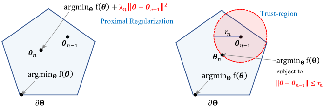
Figure 1. Illustration of the effect of proximal regularization (left) and trust-region (right).

Note that (7) is identical to BMM (2) except that we restrict the range of parameter search within a radius $r_{n}$ from the previous estimation. Our key observation is that this additional trust-region constraint can replace the role of strong convexity of surrogates, so we can use non-strongly-convex surrogates for block optimization. When $r_{n}\equiv\infty$, then this additional radius constraint becomes vacuous, and we recover the standard BMM (2). The resulting algorithm, which we call BMM with diminishing radius (BMM-DR) is stated in Algorithm 1. See Figure 1 for an illustration of the effect of proximal regularization and trust-region.

Related work. Asymptotic convergence to stationary points of BCD for convex $f$ has been extensively studied [30, 70, 49, 75]. It is known that BCD does not always converge to the stationary points of the non-convex objective function that is convex in each block [59], but such global convergence is guaranteed under additional assumptions: Two-block ($m=2$) or strict quasiconvexity for $m-2$ blocks [27, 28] and uniqueness of minimizer per block [8, Sec. 2.7]. Due to the additional proximal regularization, BCD-PR is guaranteed to converge to stationary points as long as the proximal surrogates $g_{n}^{(i)}$ in (4) is strongly convex (see [28, 79, 1]). In [79], it was shown that block PGD in (6) converges asymptotically to a Nash equilibrium (a weaker notion than stationary points) and also a local rate of convergence under the Kurdyka-Łojasiewicz condition is established. More generally, in [62], BMM (2) is known to converge to the set of stationary points when the surrogates $g_{n}^{(i)}$ have unique minimizer over the constraint sets $\Theta^{(i)}$.

For minimizing convex objectives, BMM reduces the gap between the current objective value and the global minimum at rate $O(1/n)$ in $n$ iterations [32], assuming strong convexity of the surrogates. A series of works including [68, 18, 12, 72, 54] proved the complexity of BMM and its variant under different settings. A summary of some tricks used in the proofs can also be found in [7]. These results, however, require certain types of convexity assumptions. For minimizing a general constrained nonconvex objective, the iteration complexity of an algorithm refers to the worst-case number of iterations until an $\varepsilon$-approximate stationary point is obtained. Compared to the convex minimization case, however, the iteration complexity for BMM (2) for constrained nonconvex setting is not very well understood. In particular, iteration complexity for BCD and block PGD is unknown, although a local linear convergence rate for block PGD was established in [76]. A Riemannian counterpart of block PGD for compact manifolds was recently shown to have iteration complexity of $\widetilde{O}(\varepsilon^{-2})$ [61]. But this result does not hold for the Euclidean setting both with or without constraints, as the underlying manifold should be compact without boundary. Recently, Lyu and Kwon showed that BCD-PR has iteration complexity of $\widetilde{O}(\varepsilon^{-2})$ [36] both for the constrained and unconstrained settings.

Contribution. In this work, we analyze the block majorization-minimization algorithm with optional trust-region constraints (7). Our main results are summarized below:

(1)

Global asymptotic convergence to stationary points from arbitrary initialization;

(2)

An upper bound on the rate of convergence to stationary points of order $n^{-1/2}\log n$;

(3)

Worst-case bound of $O(\varepsilon^{-2}(\log\varepsilon^{-1})^{2})$ on the number of iterations to achieve $\varepsilon$-approximate stationary points;

(4)

Robustness of the aforementioned results under inexact execution of the algorithm;

(5)

Allowing convex but non-strongly-convex surrogates by utilizing trust-regions with diminishing radii.

To the best of our knowledge, we believe our work provides the first result on the global rate of convergence and iteration complexity of BMM for minimizing smooth nonconvex objectives under convex constraints. We do not impose any additional assumptions such as the Kurdyka-$\L$ojasiewicz property. For gradient descent methods with unconstrained nonconvex objective, it is known that such rate of convergence cannot be faster than $O(1/n^{1/2})$ [15], so our rate bound matches the optimal result up to a $\log n$ factor. These results continue to hold if convex sub-problems are solved inexactly. We allow either using strongly convex surrogates, or convex surrogates with possibly non-unique solutions for the sub-problems together with trust-regions of diminishing radii.

We apply our framework and results to various stylized examples such as nonnegative matrix factorization (NMF), nonnegative CANDECOMP/PARAFAC-decomposition (NCPD), and block projected gradient descent (BPGD) and obtain the following results:

(6)

A regularized version of the multiplicative update algorithm for nonnegative matrix/tensor factorization with guaranteed asymptotic convergence to stationary points and iteration complexity of $O(\varepsilon^{-2}(\log\varepsilon^{-1})^{2})$;

(7)

Asymptotic convergence to stationary points and iteration complexity of $O(\varepsilon^{-2}(\log\varepsilon^{-1})^{2})$ for block projected gradient descent .

We believe that these are the first iteration complexity results for NMF and NCPD as well as BPGD for nonconvex objectives. We experimentally validate our theoretical results with both synthetic and real-world data and demonstrate. We find that that our algorithms outperform the existing ones especially when the matrix and tensors to be factorized are sparse.

Notation. Throughout this section, we will denote by $(\boldsymbol{\theta}_{n})_{n\geq 1}$ an (possibly inexact) output of Algorithm 1. Write $\boldsymbol{\theta}_{n}=[\theta^{(1)}_{n},\dots,\theta^{(m)}_{n}]$ for $n\geq 1$. Also, for each $n\geq 1$ and $i\in\{1,\dots,m\}$, we denote

(8) $$\Theta^{(i)}_{n}:=\{\theta\in\Theta^{(i)}\,|\,\lVert\theta-\theta_{n-1}^{(i)}\rVert\leq r_{n}\},$$

which is the constraint set that appears in (11).

Throughout this paper, denote $\Lambda:=\{\boldsymbol{\theta}_{n}\,|\,n\geq 1\}\subseteq\boldsymbol{\Theta}$. Also, for each $n\geq 1$, denote $\Lambda_{n}^{\star}$ the set of the exact output of one step of Algorithm 1. That is,

(9) $$\Lambda_{n}^{\star}:=\{\boldsymbol{\theta}_{n}^{\star}=[\theta_{n}^{(1\star)},\dots,\theta_{n}^{(m\star)}]\,:\,\textup{$\theta_{n}^{(i\star)}$ is an exact minimizer of $g_{n}^{(i)}$ over $\Theta^{(i)}_{n}$ for $i=1,\dots,m$}\}.$$

We will denote a generic element of $\Lambda^{\star}_{n}$ by $\boldsymbol{\theta}_{n}^{\star}$.

Organization. This paper is organized as follows. We state the algorithm (Algorithm 1) and the main results Section 2. In Section 3, we prove the iteration complexity results stated in Theorem 2.1 (i)-(ii). In Section 4, we prove the asymptotic stationary result stated in Theorem 2.1 (iii). Then we provide some applications of our theory in Section 5. Finally, we present the experimental results of the applications in Section 6.

2. Statement of main results

2.1. Statement of the algorithm

In this section, we give a formal statement of the BMM-DR algorithm (7), which entails all algorithms mentioned in the introduction: BCD (3), BCD-PR (4), and BMM (2).

Algorithm 1 Block Majorization-Minimization with Diminishing Radius (BMM-DR)

1:Input: $\boldsymbol{\theta}_{0}=(\theta_{0}^{(1)},\cdots,\theta_{0}^{(m)})\in\Theta^{(1)}\times\cdots\times\Theta^{(m)}$ (initial estimate); $N$ (number of iterations); $(r_{n})_{n\geq 1}$, (non-increasing radii in $(0,\infty]$)

2: for $n=1,\dots,N$ do:

3:  Update estimate $\boldsymbol{\theta}_{n}=[\theta_{n}^{(1)},\cdots,\theta_{n}^{(m)}]$ by

4:   For $i=1,\cdots,m$ do:  

(10) $$g_{n}^{(i)}\leftarrow\left[\textup{Majorizing surrogate of $\theta\mapsto f_{n}^{(i)}(\theta):=f\left(\theta_{n}^{(1)},\cdots,\theta_{n}^{(i-1)},\theta,\theta_{n-1}^{(i+1)},\cdots,\theta_{n-1}^{(m)}\right)$}\right]$$

(11) $$\theta_{n}^{(i)}\in\operatorname*{arg\,min}_{\theta\in\Theta^{(i)},\,\lVert\theta-\theta_{n-1}^{(i)}\rVert\leq r_{n}}\,g_{n}^{(i)}(\theta)$$

5:   end for

6: end for

7:output: $\boldsymbol{\theta}_{N}$

The majorizing surrogate $g_{n}^{(i)}$ in (10) is chosen so that

(1) (Majorization) $g_{n}^{(i)}(\theta)-f_{n}^{(i)}(\theta)\geq 0$ for all $\theta\in\Theta^{(i)}$;

(2) (Sharpness) $g_{n}^{(i)}(\theta_{n-1}^{(i)})=f_{n}^{(i)}(\theta_{n-1}^{(i)})$;

(3) (Convexity) $g_{n}^{(i)}$ is convex on $\Theta^{(i)}$.

2.2. Measure of stationarity

Recall that we say $\boldsymbol{\theta}^{*}\in\boldsymbol{\Theta}$ is a stationary point of $f$ over $\boldsymbol{\Theta}$ if

(12) $$\sup_{\boldsymbol{\theta}\in\boldsymbol{\Theta},\,\lVert\boldsymbol{\theta}-\boldsymbol{\theta}^{*}\rVert\leq 1}\,\langle-\nabla f(\boldsymbol{\theta}^{*}),\,\boldsymbol{\theta}-\boldsymbol{\theta}^{*}\rangle\leq 0,$$

where $\langle\cdot,\,\cdot\rangle$ denotes the dot project on $\mathbb{R}^{I_{1}+\dots+I_{m}}\supseteq\boldsymbol{\Theta}$. Equivalently, let $\mathcal{N}_{\boldsymbol{\Theta}}(\boldsymbol{\theta}):=\{\eta\,:\,\langle\eta,\,{\boldsymbol{\theta}^{\prime}-\boldsymbol{\theta}}\rangle\leq 0\,\,\forall\boldsymbol{\theta}^{\prime}\in\boldsymbol{\Theta}\}$ denote the normal cone of $\boldsymbol{\Theta}$ at $\boldsymbol{\theta}$. Then $\boldsymbol{\theta}^{*}$ is a stationary point of $f$ over $\boldsymbol{\Theta}$ if and only if $-\nabla f(\boldsymbol{\theta}^{*})\in\mathcal{N}_{\boldsymbol{\Theta}}(\boldsymbol{\theta})$. If $\boldsymbol{\theta}^{*}$ is in the interior of $\boldsymbol{\Theta}$, then it implies $\lVert\nabla f(\boldsymbol{\theta}^{*})\rVert=0$. For iterative algorithms, such a first-order optimality condition may hardly be satisfied exactly in a finite number of iterations, so it is more important to know how the worst-case number of iterations required to achieve an $\varepsilon$-approximate solution scales with the desired precision $\varepsilon$. More precisely, we say $\boldsymbol{\theta}^{*}\in\boldsymbol{\Theta}$ is an $\varepsilon$-approxiate stationary point of $f$ over $\boldsymbol{\Theta}$ if

(13) $$\sup_{\boldsymbol{\theta}\in\boldsymbol{\Theta},\,\lVert\boldsymbol{\theta}-\boldsymbol{\theta}^{*}\rVert\leq 1}\,\left\langle-\nabla f(\boldsymbol{\theta}^{*}),\,\boldsymbol{\theta}-\boldsymbol{\theta}^{*}\right\rangle\leq\varepsilon.$$

This notion of $\varepsilon$-approximate solution is consistent with the corresponding notion for unconstrained problems. Indeed, if $\boldsymbol{\theta}^{*}$ is an interior point of $\boldsymbol{\Theta}$, then (13) reduces to $\lVert\nabla f(\boldsymbol{\theta}^{*})\rVert\leq\varepsilon$.

There are alternative ways to define $\varepsilon$-stationary points for constrained problems. We have the equivalence between the following two stationary measures (see [3, Prop. B.1] and [65, Prop. 8.32]):

(14) $$\sup_{\boldsymbol{\theta}\in\boldsymbol{\Theta}\setminus\{\boldsymbol{\theta}^{*}\}}\,\left\langle-\nabla f(\boldsymbol{\theta}^{*}),\,\frac{\boldsymbol{\theta}-\boldsymbol{\theta}^{*}}{\lVert\boldsymbol{\theta}-\boldsymbol{\theta}^{*}\rVert}\right\rangle=\textup{dist}(\mathbf{0},\nabla f(\boldsymbol{\theta})+\mathcal{N}_{\boldsymbol{\Theta}}(\boldsymbol{\theta})),$$

where the right-hand side is a standard measure of stationarity (e.g., see [55]). The stationary measures in (14) do not behave continuously as one approaches stationary points at the boundary of the constraint set from the interior. This was partly the motivation for Davis and Drusvyatskiy to use a ‘near-stationary measure’ incorporating Moreu envelop in their seminal work for constrained stochastic optimization [20]. Namely, if this measure is small at a parameter $\boldsymbol{\theta}$, then the prox-point $\hat{\boldsymbol{\theta}}$ is close to being stationary and is near $\boldsymbol{\theta}$. From this perspective, the stationarity measure we introduced in (13) is a measure of approximate stationarity that is direct (since it does not involve an additional proximal operator) and it behaves continuously near the boundary.

For each $\varepsilon>0$ we define the worst-case iteration complexity $N_{\varepsilon}$ of an algorithm for solving (1) as

(15) $$N_{\varepsilon}:=\sup_{\boldsymbol{\theta}_{0}\in\boldsymbol{\Theta}}\,\inf\,\{n\geq 1\,|\,\text{$\boldsymbol{\theta}_{n}$ is an $\varepsilon$-approximate stationary point of $f$ over $\boldsymbol{\Theta}$}\},$$

where $(\boldsymbol{\theta}_{n})_{n\geq 0}$ is a sequence of estimates produced by the algorithm with an initial estimate $\boldsymbol{\theta}_{0}$. Note that $N_{\varepsilon}$ gives the worst-case bound on the number of iterations for an algorithm to achieve an $\varepsilon$-approximate solution due to the supremum over the initialization $\boldsymbol{\theta}_{0}$ in (15).

2.3. Assumptions

Throughout this paper, we assume the following conditions:

A1.

The constraint sets $\Theta^{(i)}\subseteq\mathbb{R}^{I_{i}}$, $i=1,\dots,m$ are nonempty, closed, and convex (but not necessarily compact) subsets in $\mathbb{R}^{I_{i}}$.

A2.

The objective function $f:\boldsymbol{\Theta}\rightarrow\mathbb{R}$ is continuously differentiable, and for each compact subset $\boldsymbol{\Theta}_{0}\subseteq\boldsymbol{\Theta}$, there exist a constant $L_{f}=L_{f}(\boldsymbol{\Theta}_{0})$ such that $\lVert\nabla f(x)-\nabla f(y)\rVert\leq L_{f}\lVert x-y\rVert$ for all $x,y\in\boldsymbol{\Theta}_{0}$. Also, $f^{*}:=\inf_{\boldsymbol{\theta}\in\boldsymbol{\Theta}}f(\boldsymbol{\theta})>-\infty$. Furthermore, the sub-level sets $f^{-1}((-\infty,a])=\{\boldsymbol{\theta}\in\boldsymbol{\Theta}\,:\,f(\boldsymbol{\theta})\leq a\}$ for $a\in\mathbb{R}$ are compact.

In A1, we allow the the constraint set $\Theta^{(i)}$ to be the whole space $\mathbb{R}^{I_{i}}$. The $C^{1}$-assumption of the objective in A2 is weaker than the $L$-smoothness assumption that is standard in the literature of BCD (see, e.g., [79, 50]).

Next, we define the majorization gap as the function $h_{n}^{(i)}:=g_{n}^{(i)}-f_{n}^{(i)}$ for each $n\geq 0$ and $i=1,\dots,m$. Note that $h_{n}^{(i)}\geq 0$, $h_{n}^{(i)}(\theta_{n-1}^{(i)})=0$. Hence if we assume $h_{n}^{(i)}$ is differentiable, then necessarily $\nabla h_{n}^{(i)}(\theta_{n-1}^{(i)})=0$. We make the following assumption for the majorization gap.

A3.

Either of the following holds:

(a)

(Trust-region used)    $\sum_{n=1}^{\infty}r_{n}^{2}<\infty$; or

(b)

(Trust-region not used)    $r_{n}\equiv\infty$ and the majorization gap $h_{n}^{(i)}$ satisfies the quadratic lower bound

(16) $$h_{n}^{(i)}(\theta)\geq\frac{\rho}{2}\lVert\theta-\theta_{n-1}^{(i)}\rVert^{2}\quad\textup{for all $\theta\in\Theta^{(i)}$}$$

for some constant $\rho>0$.

Furthermore, the majorization gap $h_{n}^{(i)}=g_{n}^{(i)}-f_{n}^{(i)}$ satisfies the following smoothness property:

(c)

For each compact subset $\boldsymbol{\Theta}_{0}\subseteq\boldsymbol{\Theta}$, there exist a constant $L_{h}=L_{h}(\boldsymbol{\Theta}_{0})$ such that $\lVert\nabla h_{n}^{(i)}(x)-\nabla h_{n}^{(i)}(y)\rVert\leq L_{h}\lVert x-y\rVert$ for all $x,y\in\boldsymbol{\Theta}_{0}$.

Note that the sub-problem of block minimization (11) amounts to minimizing convex majorizing surrogate $g_{n}^{(i)}$ over the constraint set $\Theta^{(i)}$ if $r_{n}=\infty$ or the intersection $\Theta^{(i)}\cap\{\theta\,:\,\lVert\theta-\theta_{n-1}^{(i)}\rVert\leq r_{n}\}$ if $r_{n}<\infty$, which are both convex sets. Hence each iteration of Algorithm 1 can be readily executed using standard convex optimization procedures (see, e.g., [9]). For instance, each iteration of block PGD (6) can be exactly computed given that projection onto the convex constraint set $\Theta^{(i)}$ has a closed-form expression (e.g., nonnegativity constraints or thresholding).

However, for many instances of Algorithm 1, it could be the case that the convex sub-problems can only be solved approximately. Fortunately, our analysis of Algorithm 1 allows inexact computation of solutions to the convex sub-problems, as long as the ‘optimality gaps’ are summable. To be precise, we define the optimality gap at iteration $n$ as

(17) $$\Delta_{n}=\Delta_{n}(\boldsymbol{\theta}_{0}):=\max_{1\leq i\leq m}\left(g_{n}^{(i)}(\theta^{(i)}_{n})-g_{n}^{(i)}(\theta_{n}^{(i\star)})\right)\quad\textup{where \,\, $\theta_{n}^{(i\star)}\in\operatorname*{arg\,min}_{\theta\in\Theta^{(i)},\,\lVert\theta-\theta^{(i)}_{n-1}\rVert\leq r_{n}}g_{n}^{(i)}(\theta)$}.$$

Then we require the following summability of optimality gaps as in A4.

A4.

The optimality gaps are summable: $\sum_{n=1}^{\infty}\Delta_{n}<\infty$.

Since the sub-problems (11) are convex, they can be solved approximately up to arbitrary prescribed precision. Hence A4 can easily be satisfied. For instance, the optimality gap shrinks linearly fast if the sub-problems (11) are strongly convex by using coordinate descent algorithms or using gradient descent algorithms, where also superlinear convergence is available using accelerated methods under additional assumptions [77, 6]. We also remark that the accumulated optimality gap $\sum_{n=1}^{\infty}\Delta_{n}$ only affects the multiplicative constant in the rate of convergence in Theorem 2.1(i) but not the order of the rate.

For establishing asymptotic stationarity of the iterates produced by Algorithm 1, we need the additional assumption on the smoothness of surrogates:

A5.

(a)

(Trust-region used)    If $\sum_{n=1}^{\infty}r_{n}^{2}<\infty$, then $r_{n+1}/r_{n}=O(1)$;

(b)

(Trust-region not used)    If $r_{n}\equiv\infty$, then surrogates $g_{n}^{(i)}$ for all $n,i$ have $L_{g}$-Lipschitz contiuous gradients for some constant $L_{g}>0$ and are $\lambda$-strongly convex for some constant $\lambda>0$: For all $\theta,\theta^{*}\in\Theta^{(i)}$,

(18) $$\textup{(Lipschitz gradients)}\hskip 85.35826pt\lVert\nabla g_{n}^{(i)}(\theta)-\nabla g_{n}^{(i)}(\theta^{*})\rVert \leq L_{g}\lVert\theta-\theta^{*}\rVert,$$

(19) $$\textup{(Strong convexity)}\hskip 29.30629ptg_{n}^{(i)}(\theta)-g_{n}^{(i)}(\theta^{*})-\langle\nabla g_{n}^{(i)}(\theta^{*}),\,\theta-\theta^{*}\rangle \geq\frac{\lambda}{2}\lVert\theta-\theta^{*}\rVert^{2}.$$

We remark that in case $g_{n}^{(i)}=f_{n}^{(i)}$ for all $n\geq 1$ and $i=1,\dots,m$ (i.e., zero majorization gap), in which case Algorithm 1 reduces to block coordinate descent with diminishing radius, (18) is automatically satisfied due to Proposition 3.3. We also remark that it is straightforward to extend our analysis to the case where the constants $L_{g}$ in (18) and $\lambda$ in (19) depend on the block index $i$. For simplicity of presentation, we do not pursue this straightforward generalization.

2.4. Statement of main results

Now we state the main result, Theorem 2.1. To our best knowledge, this gives the first worst-case rate of convergence and iteration complexity of BCD-type algorithms for nonconvex-constrained minimization in the literature.

Theorem 2.1.

Assume A1-A4 hold. Let $(\boldsymbol{\theta}_{n})_{n\geq 0}$ be an (possibly inexact) output of Algorithm 1. Then the following hold:

(i)

(Rate of convergence) There exists constants $M_{1},M_{2}>0$ such that for $n\geq 1$,

(20) $$\min_{1\leq k\leq n}\,\,\left[\sup_{\boldsymbol{\theta}\in\boldsymbol{\Theta},\,\lVert\boldsymbol{\theta}-\boldsymbol{\theta}_{k}\rVert\leq 1}\left\langle-\nabla f(\boldsymbol{\theta}_{k}),\,\boldsymbol{\theta}-\boldsymbol{\theta}_{k}\right\rangle\right] \leq\begin{cases}\frac{M_{1}}{\sum_{k=1}^{n}\min\{r_{k},1\}}&\textup{if $\sum_{n=1}^{\infty}r_{n}^{2}<\infty$}\\[5.0pt] \frac{M_{2}\log n}{2\sqrt{n}}&\textup{if $r_{n}\equiv\infty$}\end{cases}$$

(See (64)-(65) for explicit expressions for $M_{1}$ and $M_{2}$.)

(ii)

(Worst-case iteration complexity) Suppose either $r_{n}=1/(\sqrt{n}\log n)$ for $n\geq 1$ or $r_{n}\equiv\infty$. Then the worst-case iteration complexity $N_{\varepsilon}$ for Algorithm 1 satisfies $N_{\varepsilon}=O(\varepsilon^{-2}(\log\varepsilon^{-1})^{2})$.

(iii)

(Asymptotic stationarity) Further assume that A5 holds and $\sum_{n=1}^{\infty}r_{n}=\infty$. Then $(\boldsymbol{\theta}_{n})_{n\geq 1}$ converges to the set of stationary points of $f$ over $\boldsymbol{\Theta}$.

Theorem 2.1(i) provides a bound on the rate of convergence measured in terms of the stationarity measure introduced in (13). The result covers both options when trust-regions of square-summable radii are used or trust-region is not used throughout the iterations. These two options give the same upper bound on the rate of convergence $O(n^{-1/2}\log n)$. To see this, note that the upper bound in (116) when $\sum_{n=1}^{\infty}r_{n}^{2}<\infty$ is optimized when $r_{k}$’s are chosen as large as possible. One such choice is $r_{n}=1/(\sqrt{n}\log n)$ for $n\geq 1$, which gives

(21) $$\frac{1}{\sum_{k=1}^{n}\min\{r_{k},1\}}=O(n^{-1/2}\log n).$$

In particular, if all stationary points of $f$ in $\boldsymbol{\Theta}$ are in the interior of $\boldsymbol{\Theta}$, then (116) and (21) imply

(22) $$\min_{1\leq k\leq n}\,\lVert\nabla f(\boldsymbol{\theta}_{k})\rVert=O\left(n^{-1/2}\log n\right).$$

This matches the worst-case rate of convergence in gradient norm for first-order methods for unconstrained nonconvex optimization [11, 71, 80, 78, 38].

Theorem 2.1(ii) gives a worst-case iteration complexity of Algorithm 1 of producing and $\varepsilon$-stationary point. This can be easily obtained from Theorem 2.1(i) by setting the upper bound to be less than $\varepsilon$.

Lastly, Theorem 2.1(iii) states that the iterates produced by Algorithm 1, possibly solving the sub-problems inexactly with summable optimality gap, asymptotically converges to the set of stationary points of the problem (1). In the special case when all stationary points of $f$ over $\boldsymbol{\Theta}$ are isolated, then global convergence to a single stationary point can be easily deduced from Theorem 2.1(iii).

The most technical part of our asymptotic analysis is to handle inexact computation when bounded trust-regions are used. Roughly speaking, for asymptotic analysis with trust-region, we need to show that the additional trust-region constraints ‘vanish’ in the limit in the sense that any convergent subsequence of the iterates cannot touch the trust-region boundaries indefinitely. Allowing inexact computation of the surrogate minimization within the trust-region poses an additional challenge. The analysis is given in Section 4.

3. Proof of iteration complexity

We start by recalling a classical lemma on the first-order approximation of functions with Lipshitz gradients.

Lemma 3.1 (First-order approximation of functions with Lipschitz gradient).

Let $f:\Omega(\subseteq\mathbb{R}^{p})\rightarrow\mathbb{R}$ be differentiable and $\nabla f$ be $L$-Lipschitz continuous on $\Omega$. Then for each $\theta,\theta^{\prime}\in\Omega$,

(23) $$\left|f(\theta^{\prime})-f(\theta)-\nabla f(\theta)^{T}(\theta^{\prime}-\theta)\right|\leq\frac{L}{2}\lVert\theta-\theta^{\prime}\rVert^{2}.$$

Proof.

This is a classical lemma. See [53, Lem 1.2.3]. ∎

We will also use the following basic observation frequently: For all $n\geq 1$ and $i=1,\dots,m$,

(24) $$f^{(i)}_{n}(\theta^{(i)}_{n-1})-f^{(i)}_{n}(\theta^{(i)}_{n}) \overset{(a)}{=}g^{(i)}_{n}(\theta^{(i)}_{n-1})-g^{(i)}_{n}(\theta^{(i\star)}_{n})+g^{(i)}_{n}(\theta^{(i\star)}_{n})-g^{(i)}_{n}(\theta^{(i)}_{n})+g^{(i)}_{n}(\theta^{(i)}_{n})-f^{(i)}_{n}(\theta^{(i)}_{n})$$

(25) $$\overset{(b)}{\leq}-\Delta_{n}+g^{(i)}_{n}(\theta^{(i)}_{n})-f^{(i)}_{n}(\theta^{(i)}_{n})$$

(26) $$\overset{(c)}{\leq}-\Delta_{n},$$

where (a) follows from $g_{n}^{(i)}(\theta_{n-1}^{(i)})=f_{n}^{(i)}(\theta_{n-1}^{(i)})$, (b) follows from the definition of $\Delta_{n}$ in (17), and (c) follows from that $g_{n}^{(i)}$ majorizes $f_{n}^{(i)}$.

Proposition 3.2 (Monotonicity of objective and Stability of iterates).

Suppose A1, A2, and A4 hold. Then the following hold:

(i)

$f(\boldsymbol{\theta}_{n-1})-f(\boldsymbol{\theta}_{n})\geq-m\Delta_{n}+\sum_{i=1}^{m}h^{(i)}_{n}(\theta^{(i)}_{n})\geq-m\Delta_{n}$;

(ii)

$\sum_{n=1}^{\infty}\sum_{i=1}^{m}h^{(i)}_{n}(\theta^{(i)}_{n})<f(\boldsymbol{\theta}_{0})-f^{*}+m\sum_{n=1}^{\infty}\Delta_{n}<\infty$.

(iii)

If $\sum_{n=1}^{\infty}r_{n}^{2}<\infty$, then $\lVert\theta_{n}^{(i)}-\theta_{n-1}^{(i)}\rVert\leq r_{n}$ for all $i,n$ and

(27) $$\sum_{n=1}^{\infty}\lVert\boldsymbol{\theta}_{n}-\boldsymbol{\theta}_{n-1}\rVert^{2}\leq\sum_{n=1}^{\infty}r_{n}^{2}<\infty.$$

If $h_{n}^{(i)}(\theta)\geq\frac{\rho}{2}\lVert\theta-\theta_{n-1}^{(i)}\rVert^{2}$ for all $\theta\in\Theta^{(i)}$ and for all $i,n$, then

(28) $$\frac{\rho}{2}\sum_{n=1}^{\infty}\lVert\boldsymbol{\theta}_{n}-\boldsymbol{\theta}_{n-1}\rVert^{2} \leq\sum_{n=1}^{\infty}\sum_{i=1}^{m}h^{(i)}_{n}(\theta^{(i)}_{n})<f(\boldsymbol{\theta}_{0})-f^{*}+m\sum_{n=1}^{\infty}\Delta_{n}<\infty.$$

In particular, in both cases, $\lVert\theta_{n-1}^{(i)}-\theta_{n}^{(i)}\rVert=o(1)$ for all $i=1,\dots,m$.

Proof.

Fix $i\in\{1,\dots,m\}$. By (24), it follows that

(29) $$f(\boldsymbol{\theta}_{n-1})-f(\boldsymbol{\theta}_{n})$$

(30) $$\qquad=\sum_{i=1}^{m}f(\theta_{n}^{(1)},\dots,\theta_{n}^{(i-1)},\theta_{n-1}^{(i)},\theta_{n-1}^{(i+1)},\dots,\theta_{n-1}^{(m)})-f(\theta_{n}^{(1)},\dots,\theta_{n}^{(i-1)},\theta_{n}^{(i)},\theta_{n-1}^{(i+1)},\dots,\theta_{n-1}^{(m)})$$

(31) $$\qquad=\sum_{i=1}^{m}f_{n}^{(i)}(\theta^{(i)}_{n-1})-f_{n}^{(i)}(\theta^{(i)}_{n})$$

(32) $$\qquad\geq-m\Delta_{n}+\sum_{i=1}^{m}g^{(i)}_{n}(\theta^{(i)}_{n})-f^{(i)}_{n}(\theta^{(i)}_{n})$$

(33) $$\qquad\geq-m\Delta_{n}.\quad$$

This shows (i). Note that (ii) follows by adding up the above inequality for $n\geq 1$.

Lastly, we show (iii). If $\sum_{n=1}^{\infty}r_{n}^{2}<\infty$, then the assertion follows immediately. Otherwise, suppose the majorization gap $h_{n}^{(i)}$ satisfies the quadratic lower bound. Then by (16),

(34) $$g^{(i)}_{n}(\theta^{(i)}_{n})-f^{(i)}_{n}(\theta^{(i)}_{n}) \geq\frac{\rho}{2}\lVert\theta_{n}^{(i)}-\theta_{n-1}^{(i)}\rVert^{2}.$$

Together with (ii) we get (iii). ∎

Proposition 3.3 (Boundedness of iterates).

Assume A1, A2, A4, and either A3(a) or A3(b) hold (but not necessarily A3(c)). Then there exists compact and convex subsets $S^{(i)}\subseteq\Theta^{(i)}$ for $i=1,\dots,m$ such that

(35) $$\bigcup_{n=0}^{\infty}B_{\leq 1}(\boldsymbol{\theta}_{n})\subseteq\boldsymbol{\Theta}_{0}:=S^{(1)}\times\dots\times S^{(m)},$$

where $B_{\leq 1}(x):=\{y\in\boldsymbol{\Theta}\,:\,\lVert x-y\rVert\leq 1\}$.

Proof.

First let $T:=m\sum_{k=1}^{\infty}\Delta_{k}$, which is finite by A4. Recall that by Proposition 3.2, we have

(36) $$\sup_{n\geq 0}f(\boldsymbol{\theta}_{n})\leq f(\boldsymbol{\theta}_{0})+T<\infty.$$

It follows that $\{\boldsymbol{\theta}_{n}\,:\,n\geq 0\}$ is a subset of the sublevel set $A_{0}:=f^{-1}((-\infty,f(\boldsymbol{\theta}_{0})+T])$, which is compact by A2. Let $\Pi^{(i)}$ denote the projection from $\boldsymbol{\Theta}$ to its $i$th block component $\Theta^{(i)}$. Then $\Pi^{(i)}(A_{0})$ is a compact subset of $\Theta^{(i)}$. Take $R^{(i)}$ to be the ‘unit fattening’ of this compact subset, that is,

(37) $$R^{(i)}:=\left\{\theta\in\Theta^{(i)}\,:\,\lVert\theta-\theta^{\prime}\rVert\leq 1\,\,\textup{for some $\theta^{\prime}\in\Pi^{(i)}(A_{0})$}\right\}.$$

Now let $S^{(i)}$ be the convex hull of $R^{(i)}$ for $i=1,\dots,m$. Then $S^{(i)}$ is closed and bounded, so is also a compact subset of $\Theta^{(i)}$. Then (35) follows for $\boldsymbol{\Theta}_{0}:=S^{(1)}\times\dots\times S^{(m)}$. ∎

Proposition 3.4 (Finite first variation I).

Assume A1-A4 hold and let $L=L_{f}>0$ be as in Proposition 3.3. Suppose $\sum_{n=1}^{\infty}r_{n}^{2}<\infty$. Then

$$\sum_{n=0}^{\infty}\left|\left\langle\nabla f(\boldsymbol{\theta}_{n+1}),\,\boldsymbol{\theta}_{n}-\boldsymbol{\theta}_{n+1}\right\rangle\right| \leq\begin{cases}\frac{L}{2}\sum_{n=1}^{\infty}r_{n}^{2}+\left(f(\boldsymbol{\theta}_{0})-f^{*}\right)+\left(\frac{L}{\rho}+2\right)m\sum_{n=1}^{\infty}\Delta_{n}<\infty&\textup{if \ref{assumption:A3}{(a)} holds,}\\[5.0pt] \left(\frac{L}{\rho}+1\right)\left(f(\boldsymbol{\theta}_{0})-f^{*}\right)+\left(\frac{L}{\rho}+2\right)m\sum_{n=1}^{\infty}\Delta_{n}<\infty&\textup{if \ref{assumption:A3}{(b)} holds.}\end{cases}$$

Proof.

By A2 and Proposition 3.3, $\nabla f$ is $L$-Lipschitz continuous on the compact subset $\boldsymbol{\Theta}_{0}\subseteq\boldsymbol{\Theta}$ (in Prop. 3.3) that contains all iterates $\boldsymbol{\theta}_{n}$, $n\geq 0$. Hence by Lemma 3.1, for all $n\geq 0$,

$$\left|f(\boldsymbol{\theta}_{n})-f(\boldsymbol{\theta}_{n+1})-\left\langle\nabla f(\boldsymbol{\theta}_{n+1}),\,\boldsymbol{\theta}_{n}-\boldsymbol{\theta}_{n+1}\right\rangle\right|\leq\frac{L}{2}\lVert\boldsymbol{\theta}_{n}-\boldsymbol{\theta}_{n+1}\|^{2}.$$

By Proposition 3.2, $f(\boldsymbol{\theta}_{n})\geq f(\boldsymbol{\theta}_{n+1})-m\Delta_{n+1}$ for each $n\geq 0$. Hence it follows that

(38) $$\left|\left\langle\nabla f(\boldsymbol{\theta}_{n+1}),\,\boldsymbol{\theta}_{n}-\boldsymbol{\theta}_{n+1}\right\rangle\right| \leq\frac{L}{2}\lVert\boldsymbol{\theta}_{n}-\boldsymbol{\theta}_{n+1}\|^{2}+|f(\boldsymbol{\theta}_{n})-f(\boldsymbol{\theta}_{n+1})|$$

(39) $$\leq\frac{L}{2}\lVert\boldsymbol{\theta}_{n}-\boldsymbol{\theta}_{n+1}\|^{2}+f(\boldsymbol{\theta}_{n})-f(\boldsymbol{\theta}_{n+1})+2m\Delta_{n+1}.$$

for $n\geq 0$. Adding up the above inequality for all $n\geq 0$ and using Proposition 3.2 then gives the assertion. ∎

The following result is the key lemma for establishing the iteration complexity of our algorithm.

Lemma 3.5 (Key lemma for iteration complexity).

Assume A1-A4 hold and let $L>0$ be as in Proposition 3.3. Let $b_{n}\in[0,\min\{r_{n},1\}]$ for all $n\geq 1$. Then for all $n\geq 0$,

(40) $$b_{n+1}\sup_{\boldsymbol{\theta}\in\boldsymbol{\Theta},\,\lVert\boldsymbol{\theta}-\boldsymbol{\theta}_{n}\rVert\leq 1}\left\langle-\nabla f(\boldsymbol{\theta}_{n}),\,\boldsymbol{\theta}-\boldsymbol{\theta}_{n}\right\rangle \leq\left\langle-\nabla f(\boldsymbol{\theta}_{n+1}),\,\boldsymbol{\theta}_{n+1}-\boldsymbol{\theta}_{n}\right\rangle+mLb_{n+1}\lVert\boldsymbol{\theta}_{n}-\boldsymbol{\theta}_{n+1}\rVert$$

(41) $$\qquad+\left(\frac{L}{2}+mL\right)\lVert\boldsymbol{\theta}_{n+1}-\boldsymbol{\theta}_{n}\rVert^{2}+\frac{Lb_{n+1}^{2}}{2}+m\Delta_{n+1},$$

for some constant $L>0$.

Proof.

Fix $n\geq 0$ and let $\boldsymbol{\theta}=[\theta^{(1)},\dots,\theta^{(m)}]\in\boldsymbol{\Theta}$ be such that $\lVert\boldsymbol{\theta}-\boldsymbol{\theta}_{n}\rVert\leq b_{n+1}\leq r_{n+1}$. Then we have

(42) $$g_{n+1}^{(i)}(\theta^{(i)}_{n+1})-\Delta_{n+1} \leq g_{n+1}^{(i)}(\theta^{(i\star)}_{n+1})\leq g_{n+1}^{(i)}(\theta^{(i)}).$$

Let $\boldsymbol{\Theta}_{0}=S^{(1)}\times\dots\times S^{(m)}$ be as in Proposition 3.3. Then $\boldsymbol{\theta},\boldsymbol{\theta}_{n}\in\boldsymbol{\Theta}_{0}$ for all $n\geq 0$. From A2 and A3(c), each surrogate $g_{n}^{(i)}$ has $L$-Lipschitz continuous gradient on $S^{(i)}$ where $L=L_{f}+L_{h}>0$. Recall that $\nabla g_{n+1}^{(i)}(\theta_{n}^{(i)})=\nabla f_{n+1}^{(i)}(\theta_{n}^{(i)})$ since $g_{n}^{(i)}\geq f_{n}^{(i)}$ and $g_{n+1}^{(i)}(\theta_{n}^{(i)})=f_{n+1}^{(i)}(\theta_{n}^{(i)})$. Hence by subtracting $f_{n+1}^{(i)}(\theta_{n}^{(i)})$ from both sides and applying the $L$-smoothness of $g_{n+1}^{(i)}$ on $S^{(i)}$ (see Lemma 3.1), we get

(43) $$\left\langle\nabla f_{n+1}^{(i)}(\theta_{n}^{(i)}),\,\theta_{n+1}^{(i)}-\theta_{n}^{(i)}\right\rangle \leq\left\langle\nabla f_{n+1}^{(i)}(\theta_{n}^{(i)}),\,\theta^{(i)}-\theta_{n}^{(i)}\right\rangle$$

(44) $$\qquad+\frac{L}{2}\lVert\theta_{n+1}^{(i)}-\theta_{n}^{(i)}\rVert^{2}+\frac{L}{2}\lVert\theta^{(i)}-\theta_{n}^{(i)}\rVert^{2}+\Delta_{n+1}$$

for some constant $L>0$. Adding up these inequalities for $i=1,\dots,m$ ,

(45) $$\left\langle\left[\nabla f_{n+1}^{(1)}(\theta_{n}^{(1)}),\dots,\nabla f_{n+1}^{(m)}(\theta_{n}^{(m)})\right],\,\boldsymbol{\theta}_{n+1}-\boldsymbol{\theta}_{n}\right\rangle \leq\left\langle\left[\nabla f_{n+1}^{(1)}(\theta_{n}^{(1)}),\dots,\nabla f_{n+1}^{(m)}(\theta_{n}^{(m)})\right],\,\boldsymbol{\theta}-\boldsymbol{\theta}_{n}\right\rangle$$

(46) $$+\frac{L}{2}\lVert\boldsymbol{\theta}_{n+1}-\boldsymbol{\theta}_{n}\rVert^{2}+\frac{L}{2}\lVert\boldsymbol{\theta}-\boldsymbol{\theta}_{n}\rVert^{2}+m\Delta_{n+1}.$$

Since for each $i=1,\dots,m$ $\nabla_{i}f$ is $L$-Lipschitz in the $i$th block coordinate (Proposition 3.3), we have

(47) $$\lVert\nabla_{i}f(\boldsymbol{\theta}_{n+1})-\nabla f_{n+1}^{(i)}(\theta_{n}^{(i)})\rVert \leq L\lVert\boldsymbol{\theta}_{n}-\boldsymbol{\theta}_{n+1}\rVert,$$

(48) $$\lVert\nabla_{i}f(\boldsymbol{\theta}_{n})-\nabla f_{n+1}^{(i)}(\theta_{n}^{(i)})\rVert \leq L\lVert\boldsymbol{\theta}_{n}-\boldsymbol{\theta}_{n+1}\rVert.$$

Hence we have

(49) $$\left\langle\nabla f(\boldsymbol{\theta}_{n+1}),\,\boldsymbol{\theta}_{n+1}-\boldsymbol{\theta}_{n}\right\rangle \leq\left\langle\nabla f(\boldsymbol{\theta}_{n}),\,\boldsymbol{\theta}-\boldsymbol{\theta}_{n}\right\rangle+mL\lVert\boldsymbol{\theta}_{n}-\boldsymbol{\theta}_{n+1}\rVert\cdot\lVert\boldsymbol{\theta}-\boldsymbol{\theta}_{n}\rVert$$

(50) $$\qquad+\left(\frac{L}{2}+mL\right)\lVert\boldsymbol{\theta}_{n+1}-\boldsymbol{\theta}_{n}\rVert^{2}+\frac{L}{2}\lVert\boldsymbol{\theta}-\boldsymbol{\theta}_{n}\rVert^{2}+m\Delta_{n+1}.$$

The above holds for all $\boldsymbol{\theta}\in\boldsymbol{\Theta}$ with $\lVert\boldsymbol{\theta}-\boldsymbol{\theta}_{n}\rVert\leq b_{n+1}$. Thus we obtain

(51) $$\left\langle\nabla f(\boldsymbol{\theta}_{n+1}),\,\boldsymbol{\theta}_{n+1}-\boldsymbol{\theta}_{n}\right\rangle \leq\inf_{\boldsymbol{\theta}\in\boldsymbol{\Theta},\,\lVert\boldsymbol{\theta}-\boldsymbol{\theta}_{n}\rVert\leq b_{n+1}}\left\langle\nabla f(\boldsymbol{\theta}_{n}),\,\boldsymbol{\theta}-\boldsymbol{\theta}_{n}\right\rangle+mLb_{n+1}\lVert\boldsymbol{\theta}_{n}-\boldsymbol{\theta}_{n+1}\rVert$$

(52) $$\qquad+\left(\frac{L}{2}+mL\right)\lVert\boldsymbol{\theta}_{n+1}-\boldsymbol{\theta}_{n}\rVert^{2}+\frac{Lb_{n+1}^{2}}{2}+m\Delta_{n+1}.$$

Now observe that by the convexity of $\boldsymbol{\Theta}$, if $\boldsymbol{\theta}_{n}+av\in\boldsymbol{\Theta}$ for a scalar $a\geq 1$ and $v\in\mathbb{R}^{p}$, then $\boldsymbol{\theta}_{n}+v\in\boldsymbol{\Theta}$. Hence we get

(53) $$\sup_{\lVert u\rVert\leq 1,\,\boldsymbol{\theta}_{n}+u\in\boldsymbol{\Theta}}\left\langle-\nabla f(\boldsymbol{\theta}_{n}),\,u\right\rangle =\sup_{\lVert v\rVert\leq b_{n+1},\,\boldsymbol{\theta}_{n}+b_{n+1}^{-1}v\in\boldsymbol{\Theta}}\left\langle-\nabla f(\boldsymbol{\theta}_{n}),\,b_{n+1}^{-1}v\right\rangle$$

(54) $$\leq b_{n+1}^{-1}\sup_{\lVert v\rVert\leq b_{n+1},\,\boldsymbol{\theta}_{n}+v\in\boldsymbol{\Theta}}\left\langle-\nabla f(\boldsymbol{\theta}_{n}),\,v\right\rangle.$$

Combining the above with (51) then shows the assertion. ∎

Lemma 3.6 (Basic lemma on summability of nonnegative sequences).

Let $(a_{n})_{n\geq 0}$ and $(b_{n})_{n\geq 0}$ be sequences of nonnegative real numbers such that $\sum_{n=0}^{\infty}a_{n}b_{n}<\infty$. Then

(55) $$\min_{1\leq k\leq n}b_{k}\leq\frac{\sum_{k=0}^{\infty}a_{k}b_{k}}{\sum_{k=1}^{n}a_{k}}=O\left(\left(\sum_{k=1}^{n}a_{k}\right)^{-1}\right).$$

Proof.

The assertion follows from noting that

(56) $$\left(\sum_{k=1}^{n}a_{k}\right)\min_{1\leq k\leq n}b_{k}\leq\sum_{k=1}^{n}a_{k}b_{k}\leq\sum_{k=1}^{\infty}a_{k}b_{k}<\infty.$$

∎

Now we are ready to derive the iteration complexity results in Theorem 2.1 (i)-(ii).

Proof of Theorem 2.1 (i)-(ii).

Suppose $b_{n}\in[0,\min\{r_{n},1\}]$ is such that $\sum_{n=1}^{\infty}b_{n}^{2}<\infty$. Introduce the following notations

(57) $$A:=f(\boldsymbol{\theta}_{0})-f^{*},\quad B:=\sum_{n=1}^{\infty}\Delta_{n},\quad C:=\sum_{n=1}^{\infty}b_{n}^{2},\quad D:=\sum_{n=1}^{\infty}\lVert\boldsymbol{\theta}_{n}-\boldsymbol{\theta}_{n-1}\rVert^{2},\quad E:=\sum_{n=1}^{\infty}r_{n}^{2}.$$

Then $A\in[0,\infty)$ by A2, $B\in[0,\infty)$ by A4, $C\in[0,\infty)$ by the hypothesis, and $D\in[0,\infty)$ by Proposition 3.2. Furthermore, by Cauchy-Schwarz inequality,

(58) $$\sum_{n=0}^{\infty}b_{n+1}\lVert\boldsymbol{\theta}_{n}-\boldsymbol{\theta}_{n+1}\rVert\leq\sqrt{CD}<\infty.$$

Now summing the inequalities in (40) in Lemma 3.5 for all $n\geq 0$ and using Proposition 3.4, we get

(59) $$\sum_{n=0}^{\infty}b_{n+1}\sup_{\boldsymbol{\theta}\in\boldsymbol{\Theta},\,\lVert\boldsymbol{\theta}-\boldsymbol{\theta}_{n}\rVert\leq 1}\left\langle-\nabla f(\boldsymbol{\theta}_{n}),\,\boldsymbol{\theta}-\boldsymbol{\theta}_{n}\right\rangle$$

(60) $$\qquad\leq\sum_{n=0}^{\infty}\left\langle-\nabla f(\boldsymbol{\theta}_{n+1}),\,\boldsymbol{\theta}_{n+1}-\boldsymbol{\theta}_{n}\right\rangle+mL\sum_{n=0}^{\infty}b_{n+1}\lVert\boldsymbol{\theta}_{n}-\boldsymbol{\theta}_{n+1}\rVert$$

(61) $$\hskip 56.9055pt+\left(\frac{L}{2}+mL\right)\sum_{n=0}^{\infty}\lVert\boldsymbol{\theta}_{n+1}-\boldsymbol{\theta}_{n}\rVert^{2}+\frac{L}{2}\sum_{n=0}^{\infty}b_{n+1}^{2}$$

(62) $$\qquad\leq M<\infty,$$

where

(63) $$M:=\begin{cases}A+\left(\frac{L}{2}+3\right)mB+\frac{L}{2}C+L\left(\frac{1}{2}+m\right)D+mL\sqrt{CD}+\frac{L}{2}E&\textup{if \ref{assumption:A3}{(a)} holds,}\\ \left(\frac{L}{\rho}+1\right)A+\left(\frac{L}{2}+3\right)mB+\frac{L}{2}C+L\left(\frac{1}{2}+m\right)D+mL\sqrt{CD}&\textup{if \ref{assumption:A3}{(b)} holds}.\end{cases}$$

On one hand, suppose A3(a) holds. Then we choose $b_{n}=\min\{r_{n},1\}$ for $n\geq 1$. Then $\max\{C,D\}\leq E$, so in this case

(64) $$M\leq M_{1}:=A+\left(\frac{L}{2}+3\right)mB+L\left(\frac{3}{2}+2m\right)E.$$

On the other hand, suppose A3(b) holds. By Proposition 3.2, $D\leq\frac{2}{\rho}(A+mB)$. Hence

(65) $$M\leq M_{2}:=\left(L\left(\rho^{-1}+\rho+2m\right)+1\right)A+\left(\frac{L}{2}\left(1+\frac{2+4m}{\rho}\right)+3\right)mB+\frac{L}{2}C+mL\sqrt{C}\sqrt{\frac{2}{\rho}(A+mB)}.$$

Now Theorem 2.1 (i) is a direct consequence of (59) and Lemma 3.5.

Next, (ii) is a direct consequence of (i). Indeed, if $r_{n}=1/(\sqrt{n}\log n)$, then the upper bound on the rate of convergence in (i) is of order $O(1/\sum_{k=1}^{n}k^{-1/2}/(\log k))=O(\log n\big{/}2\int_{1}^{n}x^{-1/2}\,dx)=O(\frac{\log n}{2\sqrt{n}})$. Similarly, if $r_{n}\equiv\infty$, then we can choose $b_{n}=n^{-1/2}/(\log n)$ for $n\geq 1$. Then we have the same rate of convergence in (i). Then one can conclude by using the fact that $n\geq 2\varepsilon^{-1}(\log\varepsilon^{-1})^{2}$ implies $(\log n)^{2}/n\leq\varepsilon$ for all sufficiently small $\varepsilon>0$. ∎

4. Proof of asymptotic stationarity

Recall that after the update $\boldsymbol{\theta}_{n-1}\mapsto\boldsymbol{\theta}_{n}$, each block coordinate of $\boldsymbol{\theta}_{n}$ and $\boldsymbol{\theta}_{n}^{\star}$ are within distance $r_{n}$ from the corresponding block coordinate of $\boldsymbol{\theta}_{n-1}$. For each $n\geq 1$, we say $\boldsymbol{\theta}_{n}^{\star}$ is a short point if all of its block coordinates are strictly within $r_{n}$ from the corresponding block coordinate of $\boldsymbol{\theta}_{n-1}$, and $\boldsymbol{\theta}_{n}^{\star}$ is said to be a long point otherwise. Observe that if $\boldsymbol{\theta}_{n}^{\star}$ is a short point, then imposing the search radius restriction in (11) has no effect and $\boldsymbol{\theta}_{n}^{\star}$ is obtained from $\boldsymbol{\theta}_{n-1}$ by a single cycle of exact block majorization-minimization on the constraint set $\boldsymbol{\Theta}$. In particular, this holds if $r_{n}=\infty$ since then every $\boldsymbol{\theta}_{n}^{\star}\in\Lambda^{\star}$ must be a short point.

Proposition 4.1 (Vanishing gradient of the majorization gap).

Suppose A3(c) holds. Then there exists a constant $L_{h}>0$ such that for all $n\geq 1$ and $i=1,\dots,m$,

(66) $$\lVert\nabla h_{n}^{(i)}(\theta_{n}^{(i)})\rVert\leq L_{h}\|\theta_{n}^{(i)}-\theta_{n-1}^{(i)}\|.$$

Proof.

Write $h=h_{n}^{(i)}$. Let $\boldsymbol{\Theta}_{0}=S^{(1)}\times\dots\times S^{(m)}$ by as in Proposition 3.3. Then $\boldsymbol{\theta}_{n}\in\boldsymbol{\Theta}_{0}$ for all $n\geq 1$. Then $\nabla h$ is $L_{h}$-Lipschitz continuous on $S^{(i)}$ for some uniform constant $L_{h}>0$ by A3(c). Since $\theta_{n}^{(i)},\theta_{n-1}^{(i)}\in S^{(i)}$ and $\nabla h(\theta_{n-1}^{(i)})=0$, we get $\lVert\nabla h(\theta_{n}^{(i)})\rVert=\lVert\nabla h(\theta_{n}^{(i)})-\nabla h(\theta_{n-1}^{(i)})\rVert\leq L_{h}\|\theta_{n}^{(i)}-\theta_{n-1}^{(i)}\|$, as desired. ∎

Proposition 4.2 (Asymptotic exactness of iterates).

Suppose A1-A4 hold. Then for each $i=1,\dots,m$,

(67) $$\lVert\theta_{n}^{(i)}-\theta_{n}^{(i\star)}\rVert=o(1),$$

Proof.

Fix $i\in\{1,\dots,m\}$. There are two cases to consider. First, when A3(a) holds, (67) follows from a triangle inequality and that both $\theta_{n}^{(i)}$ and $\theta_{n}^{(i\star)}$ are within distance $r_{n}$ from $\theta_{n-1}^{(i)}$ since $r_{n}=o(1)$. Second, suppose A3(b) holds. Then by the first-order optimality (recall that $\Theta^{(i)}_{n}$ in (8) is convex)

(68) $$\langle\nabla g_{n}^{(i)}(\theta_{n}^{(i\star)}),\,\theta-\theta_{n}^{(i\star)}\rangle\geq 0\quad\textup{for all $\theta\in\Theta^{(i)}_{n}$ for all $i=1,\dots,m$. }$$

Then by $\lambda$-strong convexity of $g_{n}^{(i)}$ in A3(b),

(69) $$\frac{\lambda}{2}\lVert\theta_{n}^{(i)}-\theta_{n}^{(i\star)}\rVert^{2} \leq g_{n}^{(i)}(\theta_{n}^{(i)})-g_{n}^{(i)}(\theta_{n}^{(i\star)})-\langle\nabla g_{n}^{(i)}(\theta_{n}^{(i\star)}),\,\theta_{n}^{(i)}-\theta_{n}^{(i\star)}\rangle\leq\Delta_{n}.$$

It follows that $\lVert\theta_{n}^{(i)}-\theta_{n}^{(i\star)}\rVert\leq\sqrt{2\Delta_{n}/\lambda}$. According to A4, $\Delta_{n}=o(1)$, so we have $\lVert\theta_{n}^{(i)}-\theta_{n}^{(i\star)}\rVert=o(1)$. ∎

Proposition 4.3 (Sufficient condition for stationarity I).

Assume A1-A5 hold. If $(\boldsymbol{\theta}_{n_{k}}^{\star})_{k\geq 1}$ is a convergent subsequence of $(\boldsymbol{\theta}_{n}^{\star})_{n\geq 1}$ consisting of short points, then $\lim_{k\rightarrow\infty}\boldsymbol{\theta}_{n_{k}}=\lim_{k\rightarrow\infty}\boldsymbol{\theta}_{n_{k}}^{\star}=:\boldsymbol{\theta}_{\infty}$ and $\boldsymbol{\theta}_{\infty}$ is a stationary point of $f$ over $\boldsymbol{\Theta}$.

Proof.

Note that if $\boldsymbol{\theta}_{n}^{\star}$ is a short point, then each block coordinate $\theta_{n}^{(i\star)}$ lies in the interior of $\lVert\boldsymbol{\theta}-\boldsymbol{\theta}_{n-1}^{(i)}\rVert<r_{n}$, the trust region of radius $r_{n}$. Hence by the first-order optimality condition,

(70) $$\langle\nabla g_{n}^{(i)}(\theta_{n}^{(i\star)}),\,\theta-\theta_{n}^{(i\star)}\rangle\geq 0\quad\textup{for all $\theta\in\Theta^{(i)}$ for all $i=1,\dots,m$. }$$

We wish to show that $\boldsymbol{\theta}_{\infty}$ is a stationary point of $f$ over $\boldsymbol{\Theta}$. Denote $\boldsymbol{\theta}_{\infty}=[\theta_{\infty}^{(1)},\dots,\theta_{\infty}^{(m)}]$. Fix $i\in\{1,\dots,m\}$ and $\theta\in\Theta^{(i)}$ with $\|\theta-\theta_{\infty}^{(i)}\|\leq 1$. By Proposition 3.3 and continuous differentiability of $f$ in A2, there exists a constant $C>0$ such that $\lVert\nabla f_{n}^{(i)}(\theta_{n}^{(i)})\rVert\leq C$ for all $n,i$. Then by using Cauchy-Schwartz inequality and Proposition 4.1,

(71) $$\langle\nabla f_{n}^{(i)}(\theta_{n}^{(i)}),\,\theta-\theta_{n}^{(i)}\rangle \geq\langle\nabla f_{n}^{(i)}(\theta_{n}^{(i)}),\,\theta-\theta_{n}^{(i\star)}\rangle-\lVert\nabla f_{n}^{(i)}(\theta_{n}^{(i)})\rVert\,\lVert\theta_{n}^{(i)}-\theta_{n}^{(i\star)}\rVert$$

(72) $$\geq\langle\nabla g_{n}^{(i)}(\theta_{n}^{(i)}),\,\theta-\theta_{n}^{(i\star)}\rangle-\lVert\nabla h_{n}^{(i)}(\theta_{n}^{(i)})\rVert\,\lVert\theta-\theta_{n}^{(i)}\rVert-C\,\lVert\theta_{n}^{(i)}-\theta_{n}^{(i\star)}\rVert$$

(73) $$\geq\langle\nabla g_{n}^{(i)}(\theta_{n}^{(i)}),\,\theta-\theta_{n}^{(i\star)}\rangle-L_{h}\lVert\theta_{n}^{(i)}-\theta_{n-1}^{(i)}\rVert\,\lVert\theta-\theta_{n}^{(i)}\rVert-C\,\lVert\theta_{n}^{(i)}-\theta_{n}^{(i\star)}\rVert.$$

We apply the last inequality for $n$ replaced with $n_{k}$. By Proposition 4.2, we have $\boldsymbol{\theta}_{n_{k}}\rightarrow\boldsymbol{\theta}_{\infty}$ as $k\rightarrow\infty$. Also by Proposition 3.2, we have $\lVert\boldsymbol{\theta}_{n-1}-\boldsymbol{\theta}_{n}\rVert=o(1)$. So $\boldsymbol{\theta}_{n_{k}-1}\rightarrow\boldsymbol{\theta}_{\infty}$ as $k\rightarrow\infty$. Since $\lVert\theta-\theta_{\infty}^{(i)}\rVert\leq 1$, it follows that $\lVert\theta-\theta_{n_{k}}^{(i)}\rVert\leq 2$ for all sufficiently large $k$. Then by using continuity of $\nabla f$ and $\nabla g_{n}^{(i)}$ as well as (70), we deduce

(74) $$\langle\nabla_{i}f(\boldsymbol{\theta}_{\infty}),\,\theta-\theta_{\infty}^{(i)}\rangle =\mathop{\rm lim\,inf}\limits_{k\rightarrow\infty}\,\,\langle\nabla f_{n_{k}}^{(i)}(\theta_{n_{k}}^{(i)}),\,\theta-\theta_{n_{k}}^{(i)}\rangle$$

(75) $$\geq\mathop{\rm lim\,inf}\limits_{k\rightarrow\infty}\,\,\langle\nabla g_{n_{k}}^{(i)}(\theta_{n_{k}}^{(i\star)}),\,\theta-\theta_{n_{k}}^{(i\star)}\rangle\geq 0.$$

This holds for all $i\in\{1,\dots,m\}$ so we can conclude. ∎

Now we can deduce Theorem 2.1 (iii) for the case of BMM with strongly convex surrogates without diminishing radius.

Proof of Theorem 2.1 (iii) under A3(b).

By Proposition 3.3, the sequence of iterates $(\boldsymbol{\theta}_{n})_{n\geq 1}$ is bounded. Hence it suffices to show that every limit point of this sequence is a stationary point of $f$ over $\boldsymbol{\Theta}$. To this effect, let $(\boldsymbol{\theta}_{n_{k}})_{k\geq 1}$ denote an arbitrary convergent subsequence of $(\boldsymbol{\theta}_{n})_{n\geq 1}$. Denote $\boldsymbol{\theta}_{\infty}:=\lim_{k\rightarrow\infty}\boldsymbol{\theta}_{n_{k}}$. By Proposition 4.2, we have $\boldsymbol{\theta}_{n_{k}}^{\star}\rightarrow\boldsymbol{\theta}_{\infty}$ as $k\rightarrow\infty$. Since $r_{n}\equiv\infty$ under A3(b), each $\boldsymbol{\theta}_{n_{k}}^{\star}$ is a short point. Thus by Proposition 4.3, $\boldsymbol{\theta}_{\infty}$ is a stationary point of $f$ over $\boldsymbol{\Theta}$, as desired. ∎

In the remainder of this section, we prove Theorem 2.1(iii) under A3(a). The key technical point is to handle a sequence of iterates $(\boldsymbol{\theta}_{n})_{n\geq 1}$ where $\boldsymbol{\theta}_{n}^{\star}$ can both be short or long points due to the non-degenerate radius $r_{n}<\infty$ of the trust-region.

Proposition 4.4 (Finite first variation II).

Assume A1-A4 hold and let $L_{g}:=L_{f}+L_{h}>0$ as in Proposition 3.3. Suppose $\sum_{n=1}^{\infty}r_{n}^{2}<\infty$. Then

$$\sum_{n=0}^{\infty}\left|\left\langle\nabla f(\boldsymbol{\theta}_{n}),\,\boldsymbol{\theta}_{n}-\boldsymbol{\theta}_{n+1}^{\star}\right\rangle\right|<\infty.$$

Proof.

We first note that since $\nabla f_{n+1}^{(i)}(\theta_{n}^{(i)})=\nabla g_{n+1}^{(i)}(\theta_{n}^{(i)})$,

(76) $$\left|\left\langle\nabla f_{n+1}^{(i)}(\theta_{n}^{(i)}),\,\theta_{n}^{(i)}-\theta_{n+1}^{(i\star)}\right\rangle\right| =\left|\left\langle\nabla g_{n+1}^{(i)}(\theta_{n}^{(i)}),\,\theta_{n}^{(i)}-\theta_{n+1}^{(i\star)}\right\rangle\right|$$

(77) $$\overset{(a)}{\leq}\frac{L_{g}}{2}\lVert\theta_{n}^{(i)}-\theta_{n+1}^{(i\star)}\rVert^{2}+\left|g_{n+1}^{(i)}(\theta_{n}^{(i)})-g_{n+1}^{(i)}(\theta_{n+1}^{(i\star)})\right|$$

(78) $$\overset{(b)}{\leq}\frac{L_{g}}{2}\lVert\theta_{n}^{(i)}-\theta_{n+1}^{(i\star)}\rVert^{2}+g_{n+1}^{(i)}(\theta_{n}^{(i)})-g_{n+1}^{(i)}(\theta_{n+1}^{(i\star)})$$

(79) $$\leq\frac{L_{g}}{2}\lVert\theta_{n}^{(i)}-\theta_{n+1}^{(i\star)}\rVert^{2}+g_{n+1}^{(i)}(\theta_{n}^{(i)})-g_{n+1}^{(i)}(\theta_{n+1}^{(i)})+g_{n+1}^{(i)}(\theta_{n+1}^{(i)})-g_{n+1}^{(i)}(\theta_{n+1}^{(i\star)})$$

(80) $$\overset{(c)}{\leq}\frac{L_{g}r_{n+1}^{2}}{2}+g_{n+1}^{(i)}(\theta_{n}^{(i)})-g_{n+1}^{(i)}(\theta_{n+1}^{(i)})+\Delta_{n+1},$$

where (a) follows from Proposition 3.3 with $L_{g}:=L_{f}+L_{h}>0$, (b) follows since $\theta_{n+1}^{(i\star)}$ is an exact minimizer of $g_{n+1}^{(i)}$ over $\Theta^{(i)}_{n+1}$ and $\theta_{n}^{(i)}\in\Theta^{(i)}_{n+1}$, and (c) follows from the trust-region constraint and the definition of $\Delta_{n+1}$ in (17).

Next, recalling $g_{n+1}^{(i)}(\theta_{n}^{(i)})=f_{n+1}^{(i)}(\theta_{n}^{(i)})$ and $g_{n}^{(i)}\geq f_{n}^{(i)}$, we get

(81) $$\sum_{i=1}^{m}g_{n+1}^{(i)}(\theta_{n}^{(i)})-g_{n+1}^{(i)}(\theta_{n+1}^{(i)}) =\sum_{i=1}^{m}f_{n+1}^{(i)}(\theta_{n}^{(i)})-g_{n+1}^{(i)}(\theta_{n+1}^{(i)})$$

(82) $$\leq\sum_{i=1}^{m}f_{n+1}^{(i)}(\theta_{n}^{(i)})-f_{n+1}^{(i)}(\theta_{n+1}^{(i)})$$

(83) $$=f(\boldsymbol{\theta}_{n})-f(\boldsymbol{\theta}_{n+1}).$$

Then summing the above inequality over $n\geq 0$ is at most a telescoping sum, which is at most $f(\boldsymbol{\theta}_{0})-f^{*}$, so this shows

(84) $$\sum_{n=0}^{\infty}\sum_{i=1}^{m}g_{n+1}^{(i)}(\theta_{n}^{(i)})-g_{n+1}^{(i)}(\theta_{n+1}^{(i)})\leq f(\boldsymbol{\theta}_{0})-f^{*}.$$

Lastly, using $L_{f}$-Lipschitz continuity of $\nabla_{i}f$ for each $i=,\dots,m$ in Proposition 3.3,

(85) $$\sum_{i=1}^{m}\left|\left\langle\nabla f_{n+1}^{(i)}(\theta_{n}^{(i)}),\,\theta_{n}^{(i)}-\theta_{n+1}^{(i\star)}\right\rangle\right| \geq\left|\left\langle\nabla f_{n+1}^{(1)}(\theta_{n}^{(1)}),\dots,\nabla f_{n+1}^{(m)}(\theta_{n}^{(m)}),\,\boldsymbol{\theta}_{n}-\boldsymbol{\theta}_{n+1}^{\star}\right\rangle\right|$$

(86) $$\geq\left|\left\langle\nabla f(\boldsymbol{\theta}_{n}),\,\boldsymbol{\theta}_{n}-\boldsymbol{\theta}_{n+1}^{\star}\right\rangle\right|-mL_{f}\lVert\boldsymbol{\theta}_{n}-\boldsymbol{\theta}_{n+1}\rVert\,\lVert\boldsymbol{\theta}_{n}-\boldsymbol{\theta}_{n+1}^{\star}\rVert$$

(87) $$\geq\left|\left\langle\nabla f(\boldsymbol{\theta}_{n}),\,\boldsymbol{\theta}_{n}-\boldsymbol{\theta}_{n+1}^{\star}\right\rangle\right|-mL_{f}r_{n+1}^{2}.$$

Therefore, combining the above inequalities,

(88) $$\sum_{n=0}^{\infty}\left|\left\langle\nabla f(\boldsymbol{\theta}_{n}),\,\boldsymbol{\theta}_{n}-\boldsymbol{\theta}_{n+1}^{\star}\right\rangle\right|\leq\left(\frac{mL_{g}}{2}+mL_{f}\right)\sum_{n=1}^{\infty}r_{n}^{2}+(f(\boldsymbol{\theta}_{0})-f^{*})+m\sum_{n=1}^{\infty}\Delta_{n}<\infty,$$

as desired. ∎

Lemma 4.5 (Key lemma for asymptotic stationarity for inexact trust-region).

Assume A1-A3. Suppose $\sum_{n=1}^{\infty}r_{n}^{2}<\infty$. Then there is a constant $c>0$ such that for all $n\geq 0$,

(89) $$\min\{r_{n},1\}\sup_{\boldsymbol{\theta}\in\boldsymbol{\Theta},\,\lVert\boldsymbol{\theta}-\boldsymbol{\theta}_{n}\rVert\leq 1}\left\langle-\nabla f(\boldsymbol{\theta}_{n}),\,\boldsymbol{\theta}_{n+1}-\boldsymbol{\theta}_{n}\right\rangle \leq\left\langle-\nabla f(\boldsymbol{\theta}_{n}),\,\boldsymbol{\theta}_{n+1}^{\star}-\boldsymbol{\theta}_{n}\right\rangle+cr_{n+1}^{2}.$$

Proof.

Let $b_{n}:=\min\{r_{n},1\}$ for all $n\geq 1$. Fix $n\geq 0$ and let $\boldsymbol{\theta}=[\theta^{(1)},\dots,\theta^{(m)}]\in\boldsymbol{\Theta}$ be such that $\lVert\boldsymbol{\theta}-\boldsymbol{\theta}_{n}\rVert\leq b_{n+1}\leq r_{n+1}$. Then we have

(90) $$g_{n+1}^{(i)}(\theta^{(i\star)}_{n+1})\leq g_{n+1}^{(i)}(\theta^{(i)}).$$

Let $\boldsymbol{\Theta}_{0}=S^{(1)}\times\dots\times S^{(m)}$ be as in Proposition 3.3. From A2 and A3(c), each surrogate $g_{n}^{(i)}$ has $L$-Lipschitz continuous gradient on $S^{(i)}$ where $L=L_{f}+L_{h}>0$. Also, $\boldsymbol{\theta},\boldsymbol{\theta}_{n+1}^{\star},\boldsymbol{\theta}_{n}\in\boldsymbol{\Theta}_{0}$ for all $n\geq 1$. Recall that $\nabla g_{n+1}^{(i)}(\theta_{n}^{(i)})=\nabla f_{n+1}^{(i)}(\theta_{n}^{(i)})$ since $g_{n}^{(i)}\geq f_{n}^{(i)}$ and $g_{n+1}^{(i)}(\theta_{n}^{(i)})=f_{n+1}^{(i)}(\theta_{n}^{(i)})$. Hence by subtracting $g_{n+1}^{(i)}(\theta_{n}^{(i)})$ from both sides and applying the $L$-smoothness of $g_{n}^{(i)}$ on $S^{(i)}$ (see Lemma 3.1),

(91) $$\left\langle\nabla f_{n+1}^{(i)}(\theta_{n}^{(i)}),\,\theta_{n+1}^{(i\star)}-\theta_{n}^{(i)}\right\rangle \leq\left\langle\nabla f_{n+1}^{(i)}(\theta_{n}^{(i)}),\,\theta^{(i)}-\theta_{n}^{(i)}\right\rangle+\frac{L}{2}\lVert\theta_{n+1}^{(i\star)}-\theta_{n}^{(i)}\rVert^{2}+\frac{L}{2}\lVert\theta^{(i)}-\theta_{n}^{(i)}\rVert^{2}$$

(92) $$\leq\left\langle\nabla f_{n+1}^{(i)}(\theta_{n}^{(i)}),\,\theta^{(i)}-\theta_{n}^{(i)}\right\rangle+Lr_{n+1}^{2}.$$

Adding up these inequalities for $i=1,\dots,m$

(93) $$\sum_{i=1}^{m}\left\langle\nabla f_{n+1}^{(i)}(\theta_{n}^{(i)}),\,\theta_{n+1}^{(i\star)}-\theta_{n}^{(i)}\right\rangle \leq\left\langle\left[\nabla f_{n+1}^{(1)}(\theta_{n}^{(1)}),\dots,\nabla f_{n+1}^{(m)}(\theta_{n}^{(m)})\right],\,\boldsymbol{\theta}-\boldsymbol{\theta}_{n}\right\rangle+mLr_{n+1}^{2}$$

(94) $$\overset{(a)}{\leq}\left\langle\nabla f(\boldsymbol{\theta}_{n}),\,\boldsymbol{\theta}-\boldsymbol{\theta}_{n}\right\rangle+mL_{f}\lVert\boldsymbol{\theta}_{n+1}-\boldsymbol{\theta}_{n}\rVert\cdot\lVert\boldsymbol{\theta}-\boldsymbol{\theta}_{n}\rVert+mLr_{n+1}^{2}$$

(95) $$\overset{(b)}{\leq}\left\langle\nabla f(\boldsymbol{\theta}_{n}),\,\boldsymbol{\theta}-\boldsymbol{\theta}_{n}\right\rangle+cr_{n+1}^{2}$$

for $c:=m^{2}L_{f}+mL$, where (a) uses that $\nabla_{i}f$ is $L_{f}$-Lipschitz in the $i$th block coordinate (Proposition 3.3) for each $i=1,\dots,m$ and (b) follows since $\lVert\boldsymbol{\theta}_{n+1}-\boldsymbol{\theta}_{n}\rVert\leq mr_{n+1}$ and $\lVert\boldsymbol{\theta}-\boldsymbol{\theta}_{n}\rVert\leq r_{n+1}$. The above inequality holds for all $\boldsymbol{\theta}\in\boldsymbol{\Theta}$ with $\lVert\boldsymbol{\theta}-\boldsymbol{\theta}_{n}\rVert\leq b_{n+1}$. Furthermore, note that

(96) $$\sum_{i=1}^{m}\left\langle\nabla f_{n+1}^{(i)}(\theta_{n}^{(i)}),\,\theta_{n+1}^{(i\star)}-\theta_{n}^{(i)}\right\rangle =\left\langle\nabla f_{n+1}^{(1)}(\theta_{n}^{(1)}),\dots,\nabla f_{n+1}^{(m)}(\theta_{n}^{(1)}),\,\boldsymbol{\theta}_{n+1}^{\star}-\boldsymbol{\theta}_{n}\right\rangle$$

(97) $$\geq\left\langle\nabla f(\boldsymbol{\theta}_{n}),\,\boldsymbol{\theta}_{n+1}^{\star}-\boldsymbol{\theta}_{n}\right\rangle-mL_{f}\lVert\boldsymbol{\theta}_{n}-\boldsymbol{\theta}_{n+1}\rVert\,\lVert\boldsymbol{\theta}_{n+1}^{\star}-\boldsymbol{\theta}_{n}\rVert$$

(98) $$\geq\left\langle\nabla f(\boldsymbol{\theta}_{n}),\,\boldsymbol{\theta}_{n+1}^{\star}-\boldsymbol{\theta}_{n}\right\rangle-mL_{f}r_{n+1}^{2}.$$

Thus it follows that

(99) $$\left\langle\nabla f(\boldsymbol{\theta}_{n}),\,\boldsymbol{\theta}_{n+1}^{\star}-\boldsymbol{\theta}_{n}\right\rangle\leq\inf_{\boldsymbol{\theta}\in\boldsymbol{\Theta},\lVert\boldsymbol{\theta}-\boldsymbol{\theta}_{n}\rVert\leq b_{n+1}}\left\langle\nabla f(\boldsymbol{\theta}_{n}),\,\boldsymbol{\theta}-\boldsymbol{\theta}_{n}\right\rangle+(c+mL_{f})r_{n+1}^{2}.$$

Then using (54), we can conclude the assertion. ∎

Proposition 4.6 (Sufficient condition for stationarity II).

Assume A1-A4 hold. Suppose that $\sum_{n=1}^{\infty}r_{n}^{2}<\infty$ and $r_{n+1}/r_{n}=O(1)$. Suppose there exists a subsequence $(\boldsymbol{\theta}_{n_{k}})_{k\geq 1}$ such that for some $i\in\{1,\dots,m\}$, either

(100) $$\sum_{k=1}^{\infty}\lVert\boldsymbol{\theta}_{n_{k}}-\boldsymbol{\theta}_{n_{k}+1}^{\star}\rVert=\infty\quad\text{or}\quad\mathop{\rm lim\,inf}\limits_{k\rightarrow\infty}\,\,\left|\left\langle\nabla f(\boldsymbol{\theta}_{n_{k}}),\,\frac{\boldsymbol{\theta}_{n_{k}}-\boldsymbol{\theta}_{n_{k}+1}^{\star}}{\lVert\boldsymbol{\theta}_{n_{k}}-\boldsymbol{\theta}_{n_{k}+1}^{\star}\rVert}\right\rangle\right|=0.$$

Then there is a further subsequence $(s_{k})_{k\geq 1}$ of $(n_{k})_{k\geq 1}$ such that $\lim_{k\rightarrow\infty}\boldsymbol{\theta}_{s_{k}}$ exists and is a stationary point of $f$ over $\boldsymbol{\Theta}$.

Proof.

By Proposition 4.4,

(101) $$\sum_{k=1}^{\infty}\lVert\boldsymbol{\theta}_{n_{k}}-\boldsymbol{\theta}_{n_{k}+1}^{\star}\rVert\,\left|\left\langle\nabla f(\boldsymbol{\theta}_{n_{k}}),\,\frac{\boldsymbol{\theta}_{n_{k}}-\boldsymbol{\theta}_{n_{k}+1}^{\star}}{\lVert\boldsymbol{\theta}_{n_{k}}-\boldsymbol{\theta}_{n_{k}+1}^{\star}\rVert}\right\rangle\right|<\infty.$$

Hence the former condition in (100) implies the latter condition in (100). Thus it suffices to show that this latter condition implies the assertion. Assume this condition, and let $(t_{k})_{k\geq 1}$ be a subsequence of $(n_{k})_{k\geq 1}$ for which the liminf in (100) is achieved. By taking a further subsequence, we may assume that $\boldsymbol{\theta}_{\infty}=\lim_{k\rightarrow\infty}\boldsymbol{\theta}_{t_{k}}$ exists. Then $\boldsymbol{\theta}_{\infty}\in\boldsymbol{\Theta}$ since $\boldsymbol{\Theta}$ is closed by A1.

Now suppose for contradiction that $\boldsymbol{\theta}_{\infty}$ is not a stationary point of $f$ over $\boldsymbol{\Theta}$. Then there exists ${\boldsymbol{\theta}}^{\prime}\in\boldsymbol{\Theta}$ and $\delta>0$ such that $\left\langle\nabla f(\boldsymbol{\theta}_{\infty}),\,\boldsymbol{\theta}^{\prime}-\boldsymbol{\theta}_{\infty}\right\rangle<-\delta<0$. Denote $\boldsymbol{\theta}^{t}:=t\boldsymbol{\theta}^{\prime}+(1-t)\boldsymbol{\theta}_{\infty}$ for $t\in[0,1]$. Then

(102) $$\langle\nabla f(\boldsymbol{\theta}_{\infty}),\,\boldsymbol{\theta}^{t}-\boldsymbol{\theta}_{\infty}\rangle=t\langle\nabla f(\boldsymbol{\theta}_{\infty}),\,\boldsymbol{\theta}^{\prime}-\boldsymbol{\theta}_{\infty}\rangle<t\,\delta<0\quad\textup{for all $t\in[0,1]$}.$$

Choose $t$ sufficiently small so that $\lVert\boldsymbol{\theta}^{t}-\boldsymbol{\theta}_{\infty}\rVert<1/2$ and denote $\boldsymbol{\theta}^{*}$ for such $\boldsymbol{\theta}^{t}$. Note that $\boldsymbol{\theta}^{*}\in\boldsymbol{\Theta}$ by convexity of $\boldsymbol{\Theta}$.

By the triangle inequality, write

(103) $$\lVert\left\langle\nabla f(\boldsymbol{\theta}_{t_{k}}),\,\boldsymbol{\theta}^{*}-\boldsymbol{\theta}_{t_{k}}\right\rangle-\left\langle\nabla f(\boldsymbol{\theta}_{\infty}),\,\boldsymbol{\theta}^{*}-\boldsymbol{\theta}_{\infty}\right\rangle\rVert$$

(104) $$\qquad\leq\lVert\nabla f(\boldsymbol{\theta}_{t_{k}})-\nabla f(\boldsymbol{\theta}_{\infty})\rVert\cdot\lVert\boldsymbol{\theta}^{*}-\boldsymbol{\theta}_{t_{k}}\rVert+\lVert\nabla f(\boldsymbol{\theta}_{\infty})\rVert\cdot\lVert\boldsymbol{\theta}_{\infty}-\boldsymbol{\theta}_{t_{k}}\rVert.$$

Noting that $\lVert\boldsymbol{\theta}_{n}-\boldsymbol{\theta}_{n-1}\rVert=O(r_{n})=o(1)$, we see that the right-hand side goes to zero as $k\rightarrow\infty$. Hence by Lemma 4.5, there is a constant $c>0$ such that for al $n\geq 1$,

(105) $$\frac{\lVert\boldsymbol{\theta}_{t_{k}+1}^{\star}-\boldsymbol{\theta}_{t_{k}}\rVert}{\min\{r_{t_{k}},1\}}\left\langle\nabla f(\boldsymbol{\theta}_{t_{k}+1}^{\star}),\,\frac{\boldsymbol{\theta}_{t_{k}+1}^{\star}-\boldsymbol{\theta}_{t_{k}}}{\lVert\boldsymbol{\theta}_{t_{k}+1}^{\star}-\boldsymbol{\theta}_{t_{k}}\rVert}\right\rangle \leq\inf_{\boldsymbol{\theta}\in\boldsymbol{\Theta},\,\lVert\boldsymbol{\theta}-\boldsymbol{\theta}_{t_{k}}\rVert\leq 1}\left\langle\nabla f(\boldsymbol{\theta}_{t_{k}}),\,\boldsymbol{\theta}-\boldsymbol{\theta}_{t_{k}}\right\rangle+c\frac{r_{t_{k}+1}^{2}}{r_{t_{k}}}.$$

Since $\lVert\boldsymbol{\theta}_{n+1}^{\star}-\boldsymbol{\theta}_{n}\rVert\leq mr_{n+1}$, by using the hypothesis, the left-hand side above converges to zero as $k\rightarrow\infty$. All terms on the right-hand side above except the first one vanish as $k\rightarrow\infty$. Also note that $\lVert\boldsymbol{\theta}^{*}-\boldsymbol{\theta}_{t_{k}}\rVert\leq\lVert\boldsymbol{\theta}^{*}-\boldsymbol{\theta}_{\infty}\rVert+\lVert\boldsymbol{\theta}_{\infty}-\boldsymbol{\theta}_{t_{k}}\rVert<1$ for all $k$ sufficiently large. Hence we obtain

(106) $$0\leq\mathop{\rm lim\,inf}\limits_{k\rightarrow\infty}\inf_{\boldsymbol{\theta}\in\boldsymbol{\Theta},\,\lVert\boldsymbol{\theta}-\boldsymbol{\theta}_{t_{k}}\rVert\leq 1}\left\langle\nabla f(\boldsymbol{\theta}_{t_{k}}),\,\boldsymbol{\theta}-\boldsymbol{\theta}_{t_{k}}\right\rangle \leq\mathop{\rm lim\,inf}\limits_{k\rightarrow\infty}\,\left\langle\nabla f(\boldsymbol{\theta}_{t_{k}}),\,\boldsymbol{\theta}^{*}-\boldsymbol{\theta}_{t_{k}}\right\rangle$$

(107) $$=\left\langle\nabla f(\boldsymbol{\theta}_{\infty}),\,\boldsymbol{\theta}^{*}-\boldsymbol{\theta}_{\infty}\right\rangle<0,$$

which is a contradiction. This shows the assertion. ∎

The following proposition is crucial in establishing global convergence to stationary points (Theorem 2.1 (i)) and it is the only place where we use non-summability of the radii $r_{n}$’s in the proof of Theorem 2.1.

Proposition 4.7 (Local structure of a non-stationary limit point).

Assume A1-A4, $\sum_{n=1}^{\infty}r_{n}=\infty$, and $\sum_{n=1}^{\infty}r_{n}^{2}<\infty$. Suppose there exists a non-stationary limit point $\boldsymbol{\theta}_{\infty}$ of $\Lambda$. Then there exists $\varepsilon>0$ such that the $\varepsilon$-neighborhood $B_{\varepsilon}(\boldsymbol{\theta}_{\infty}):=\{\boldsymbol{\theta}\in\boldsymbol{\Theta}\,|\,\lVert\boldsymbol{\theta}-\boldsymbol{\theta}_{\infty}\rVert<\varepsilon\}$ with the following properties:

(a)

$B_{\varepsilon}(\boldsymbol{\theta}_{\infty})$ does not contain any stationary points of $\Lambda$.

(b)

There exists infinitely many $\boldsymbol{\theta}_{n}^{\star}$’s outside of $B_{\varepsilon}(\boldsymbol{\theta}_{\infty})$.

Proof.

Let $A$ denote the event that there exists a non-stationary limit point $\boldsymbol{\theta}_{\infty}$ of $\Lambda$. Let $B$ denote the event that there exists an $\varepsilon$-neighborhood $B_{\varepsilon}(\boldsymbol{\theta}_{\infty})$ of $\boldsymbol{\theta}_{\infty}$ that does not contain any short points of $\Lambda$. We claim that $A$ implies $B$. Suppose for contrary that $A\setminus B$ is true. Then for all $\varepsilon>0$, $B_{\varepsilon}(\boldsymbol{\theta}_{\infty})$ contains some short point of $\Lambda$. Then there exists a subsequence of short points of $\Lambda$ converging to $\boldsymbol{\theta}_{\infty}$, but then $\boldsymbol{\theta}_{\infty}$ has to be stationary by Proposition 4.3. This contradicts $A$. Hence $A$ implies $B$.

Next, on the event $A$, we show that there exists $\varepsilon>0$ such that $B_{\varepsilon}(\boldsymbol{\theta}_{\infty})$ satisfies (a). Suppose for contradiction that there exists no such $\varepsilon>0$. Then we have a sequence $(\boldsymbol{\theta}_{\infty;k})_{k\geq 1}$ of stationary points of $\Lambda$ that converges to $\boldsymbol{\theta}_{\infty}$. Fix $\boldsymbol{\theta}\in\boldsymbol{\Theta}$ and note that by Cauchy-Schwarz inequality,

(108) $$\langle\nabla f(\boldsymbol{\theta}_{\infty}),\,\boldsymbol{\theta}-\boldsymbol{\theta}_{\infty}\rangle \geq-\lVert\nabla f(\boldsymbol{\theta}_{\infty})-\nabla f(\boldsymbol{\theta}_{\infty;k})\rVert\cdot\lVert\boldsymbol{\theta}-\boldsymbol{\theta}_{\infty}\rVert$$

(109) $$\qquad-\lVert\nabla f(\boldsymbol{\theta}_{\infty;k})\rVert\cdot\lVert\boldsymbol{\theta}_{\infty}-\boldsymbol{\theta}_{\infty;k}\rVert+\langle\nabla f(\boldsymbol{\theta}_{\infty;k}),\,\boldsymbol{\theta}-\boldsymbol{\theta}_{\infty;k}\rangle.$$

Note that $\nabla f$ is continuous by A2 and $\langle\nabla f_{\infty;k}(\boldsymbol{\theta}_{\infty;k}),\,\boldsymbol{\theta}-\boldsymbol{\theta}_{\infty;k}\rangle\geq 0$ since $\boldsymbol{\theta}_{\infty;k}$ is a stationary point of $f_{\infty;k}$ over $\boldsymbol{\Theta}$. Hence by taking $k\rightarrow\infty$, this shows $\langle\nabla f(\boldsymbol{\theta}_{\infty}),\,\boldsymbol{\theta}-\boldsymbol{\theta}_{\infty}\rangle\geq 0$. Since $\boldsymbol{\theta}\in\boldsymbol{\Theta}$ was arbitrary, this implies that $\boldsymbol{\theta}_{\infty}$ is a stationary point of $f$ over $\boldsymbol{\Theta}$. This contradicts $A$.

Lastly, from the earlier results, on the event $A$, we can choose $\varepsilon>0$ such that $B_{\varepsilon}(\boldsymbol{\theta}_{\infty})$ has no short point of $\Lambda$ and also satisfies (a). We will show that $B_{\varepsilon/2}(\boldsymbol{\theta}_{\infty})$ satisfies (b). Then $B_{\varepsilon/2}(\boldsymbol{\theta}_{\infty})$ satisfies (a)-(b), as desired. Suppose for contradiction there are only finitely many $\boldsymbol{\theta}_{n}^{\star}$’s outside of $B_{\varepsilon/2}(\boldsymbol{\theta}_{\infty})$. Then there exists an integer $M\geq 1$ such that $\boldsymbol{\theta}_{n}^{\star}\in B_{\varepsilon/2}(\boldsymbol{\theta}_{\infty})$ for all $n\geq M$. Then each $\boldsymbol{\theta}_{n}^{\star}$ for $n\geq M$ is a long point of $\Lambda$. By definition, it follows that $\lVert\boldsymbol{\theta}_{n}^{\star}-\boldsymbol{\theta}_{n-1}\lVert\geq r_{n}$ for all $n\geq M$. Then since $\sum_{n=1}^{\infty}r_{n}=\infty$, by Proposition 4.6 there exists a subsequence $(n_{k})_{k\geq 1}$ such that $\boldsymbol{\theta}_{\infty}^{\prime}:=\lim_{k\rightarrow\infty}\boldsymbol{\theta}_{n_{k}}$ exists and is stationary. But since $\boldsymbol{\theta}^{\prime}_{\infty}\in B_{\varepsilon}(\boldsymbol{\theta})$, this contradicts (a). This shows the assertion. ∎

We are now ready to give proof of the asymptotic stationarity result stated in Theorem 2.1 (iii).

Proof of Theorem 2.1 (iii) under A3(a).

Suppose for contradiction that there exists a non-stationary limit point $\boldsymbol{\theta}_{\infty}\in\boldsymbol{\Theta}$ of $\Lambda$. By Proposition 4.7, we may choose $\varepsilon>0$ such that $B_{\varepsilon}(\boldsymbol{\theta}_{\infty})$ satisfies the conditions (a)-(b) of Proposition 4.7. Choose $M\geq 1$ large enough so that $r_{n}<\varepsilon/4$ whenever $t\geq M$. We call an integer interval $I:=[\ell,\ell^{\prime}]$ a crossing if $\boldsymbol{\theta}_{\ell}\in B_{\varepsilon/3}(\boldsymbol{\theta}_{\infty})$, $\boldsymbol{\theta}_{\ell^{\prime}}\in B_{2\varepsilon/3}(\boldsymbol{\theta}_{\infty})$, and no proper subset of $I$ satisfies both of these conditions. By definition, two distinct crossings have empty intersections. Fix a crossing $I=[\ell,\ell^{\prime}]$, it follows that by triangle inequality,

(110) $$\sum_{n=\ell}^{\ell^{\prime}-1}\lVert\boldsymbol{\theta}_{n+1}-\boldsymbol{\theta}_{n}\rVert\geq\lVert\boldsymbol{\theta}_{\ell^{\prime}}-\boldsymbol{\theta}_{\ell}\rVert\geq\varepsilon/3.$$

Note that since $\boldsymbol{\theta}_{\infty}$ is a limit point of $\Lambda$, $\boldsymbol{\theta}_{n}$ visits $B_{\varepsilon/3}(\boldsymbol{\theta}_{\infty})$ infinitely often. Moreover, by condition (a) of Proposition 4.7, $\boldsymbol{\theta}_{n}$ also exits $B_{\varepsilon}(\boldsymbol{\theta}_{\infty})$ infinitely often. It follows that there are infinitely many crossings. Let $t_{k}$ denote the $k^{\textup{th}}$ smallest index that appears in some crossing. Then $t_{k}\rightarrow\infty$ as $k\rightarrow\infty$, and by (110),

(111) $$\sum_{k=1}^{\infty}\lVert\boldsymbol{\theta}_{t_{k}+1}-\boldsymbol{\theta}_{t_{k}}\rVert\geq(\text{$\#$ of crossings})\,\frac{\varepsilon}{3}=\infty.$$

Then by Proposition 4.6, there exists a subsequence $(s_{k})_{k\geq 1}$ of $(t_{k})_{k\geq 1}$ such that $\boldsymbol{\theta}_{\infty}^{\prime}:=\lim_{k\rightarrow\infty}\boldsymbol{\theta}_{s_{k}}$ exists and is a stationary of $f$ over $\boldsymbol{\Theta}$. However, since $\boldsymbol{\theta}_{t_{k}}\in B_{2\varepsilon/3}(\boldsymbol{\theta}_{\infty})$ for all $k\geq 1$, we have $\boldsymbol{\theta}_{\infty}^{\prime}\in B_{\varepsilon}(\boldsymbol{\theta}_{\infty})$. This contradicts the condition (b) of Proposition 4.7 for $B_{\varepsilon}(\boldsymbol{\theta}_{\infty})$ that it cannot contain any stationary point of $f$ over $\boldsymbol{\Theta}$. This shows that there is no non-stationary limit point $\boldsymbol{\theta}_{\infty}\in\boldsymbol{\Theta}$ of $\Lambda$. See Figure 2 for an illustration of the proof. ∎

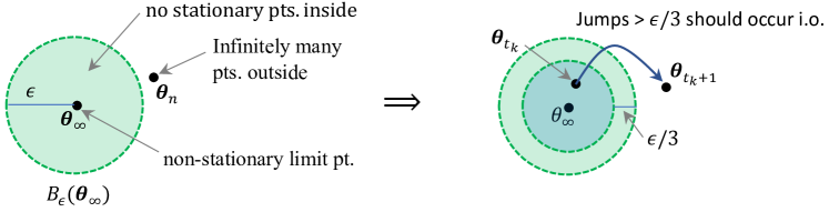
Figure 2. Illustration of the proof of Theorem 2.1 (iii) with diminishing radius.

5. Applications of the main result

5.1. Nonnegative Matrix Factorization (NMF)

Given a $p\times N$ data matrix $X\in\mathbb{R}^{p\times N}$ and an integer parameter $r\geq 1$, consider the following constrained matrix factorization problem

(112) $$\operatorname*{arg\,min}_{W\in\Theta^{(1)}\subseteq\mathbb{R}^{p\times r},\,H\in\Theta^{(2)}\subseteq\mathbb{R}^{r\times N}}\lVert X-WH\lVert_{F}^{2}+\lambda\lVert H\rVert_{1},$$

where the two factors $W$ and $H$ are called dictionary and code matrices of $X$, respectively, and $\lambda\geq 0$ is a $\ell_{1}$-regularizer for the code matrix $H$. Depending on the application contexts, we may impose some constraints $\Theta^{(1)}$ and $\Theta^{(2)}$ on the dictionary and code matrices, respectively, such as nonnegativity or some other convex constraints. An interpretation of this approximate factorization is that the $r$ columns of $W$ give an approximate basis for spanning the $N$ columns of $X$, where the columns of $H$ give suitable linear coefficients for each approximation. In dictionary learning problems [58, 25, 46, 24, 39] , one seeks for a sparse representation of the columns of $X$ with respect to and an over-complete dictionary $W$, for which one can take $r>p$ and $\lambda>0$.

The Nonnegative Matrix Factorization (NMF) [47] is a special instance of the constrain matrix factorization problem above, which is stated as follows:

(113) $$\min_{W\in\mathbb{R}_{\geq 0}^{p\times r},H\in\mathbb{R}_{\geq 0}^{r\times N}}f(W,H):=\frac{1}{2}\|X-WH\|_{F}^{2},$$

where a nonnegative data matrix $X\in\mathbb{R}_{\geq 0}^{p\times N}$ is given. NMF has numerous applications in text analysis, image reconstruction, medical imaging, bioinformatics, and many other scientific fields [66, 4, 5, 19, 74, 10, 64]. The use of nonnegativity constraint in NMF is crucial in obtaining a “parts-based" representation of the input signal [45].

In [47], the following multiplicative update (MU) algorithm is studied for solving (113):

(114) $$\textbf{MU}\hskip 85.35826pt\begin{cases}H_{n+1}\leftarrow H_{n}\odot(W_{n}^{T}X)\oslash(W_{n}^{T}W_{n}H_{n})\\ W_{n+1}^{T}\leftarrow W_{n}^{T}\odot(H_{n}X^{T})\oslash(H_{n}H_{n}^{T}W_{n}^{T}),\end{cases}$$

where $\odot$ and $\oslash$ denote entry-wise multiplication and division. Given a nonnegative initialization $(W_{0},H_{0})$, the iterate (114) generates a sequence of non-negative factor matrices $(W_{n},H_{n})_{\geq 0}$. In [47], it was shown that the objective value of (113) monotonically decreases under the iterate (114), but it has not been proven that the convergence is toward the set of stationary points of (113). There are numerous works that propose modified versions of (114) and show asymptotic convergence to stationary points. [41, 57, 73, 83]. Furthermore, to the best of our knowledge, there has not been any result on the rate of convergence of any variants of MU (114).

Here we propose MU with Regularization (MUR), which falls under our BMM (Alg. 1) and satisfies the hypothesis of our main result, Theorem 2.1. Fix regularization parameters $\delta,\rho\geq 0$. (We call $\delta$ the thresholding parameter and $\rho$ the proximal regularization parameter.) Consider the following variant of MU:

(115) $$\textbf{MUR}\hskip 56.9055pt\begin{cases}\tilde{H}_{n}\leftarrow H_{n}\lor\delta,\\ H_{n+1}\leftarrow(\tilde{H}_{n}\odot(W_{n}^{T}X+\rho\tilde{H}_{n})\oslash((W_{n}^{T}W_{n}+\rho\mathbf{I})\tilde{H}_{n}),\\ \tilde{W}_{n}\leftarrow\tilde{W}_{n}\lor\delta,\\ W_{n+1}^{T}\leftarrow W_{n}^{T}\odot(H_{n}X^{T}+\rho\tilde{W}_{n}^{T})\oslash((H_{n}H_{n}^{T}+\rho\mathbf{I})\tilde{W}_{n}^{T}),\end{cases}$$

where $(\,\cdot\lor\delta)$ is the operation of taking maximum with $\delta$ entry-wise and $\mathbf{I}$ denotes the $r\times r$ identity matrix. Note that by setting $\delta=\rho=0$, (115) reduces to the standard MU in (114). The following corollary shows that the MUR (115) algorithm for NMF, as long as $\rho,\delta>0$, retains the asymptotic convergence and the rate of convergence stated in Theorem 2.1.

Corollary 5.1 (Convergence of MUR for NMF).

Fix a matrix $X\in\mathbb{R}_{\geq 0}^{p\times N}$. Let $(\boldsymbol{\theta}_{n})_{n\geq 0}$, $\boldsymbol{\theta}_{n}:=(W_{n},H_{n})$ be generated by (115) with arbitrary initialization $\boldsymbol{\theta}_{0}\in\boldsymbol{\Theta}:=\mathbb{R}_{\geq 0}^{p\times r}\times\mathbb{R}_{\geq 0}^{r\times N}$. Denote $f(W,H):=\frac{1}{2}\lVert X-WH\rVert_{F}^{2}$. Suppose the thresholding and proximal regularization parameters $\delta,\rho$ are strictly positive. Then the following hold:

(i)

(Rate of convergence) There exists an explicit constant $M>0$ such that for $n\geq 1$,

(116) $$\min_{1\leq k\leq n}\,\,\left[\sup_{\boldsymbol{\theta}\in\boldsymbol{\Theta},\,\lVert\boldsymbol{\theta}-\boldsymbol{\theta}_{k}\rVert\leq 1}\left\langle-\nabla f(\boldsymbol{\theta}_{k}),\,\boldsymbol{\theta}-\boldsymbol{\theta}_{k}\right\rangle\right] \leq\frac{M\log n}{2\sqrt{n}}.$$

(ii)

(Worst-case iteration complexity) The worst-case iteration complexity $N_{\varepsilon}$ for the MUR algorithm (115) satisfies $N_{\varepsilon}=O(\varepsilon^{-2}(\log\varepsilon^{-1})^{2})$.

(iii)

(Asymptotic stationarity) $(\boldsymbol{\theta}_{n})_{n\geq 1}$ converges to the set of stationary points of the NMF problem (112).

In order to justify Corollary 5.1, we first explain why MUR (115) can be viewed as a special instance of the BMM algorithm (Alg. 1). Consider the following convex sub-problem of (112):

(117) $$\min_{H\geq 0}\left(f_{n}(H):=\frac{1}{2}\lVert X-W_{n}H\rVert_{F}^{2}\right).$$

For any matrix $A$ and positive integer $j$ at most the number of columns in $A$, denote $A^{j}$ to be its $j$th column. Then $f_{n}(H)=\sum_{j=1}^{N}f_{n}^{j}(H^{j})$, where $f_{n}^{j}(\mathbf{h}):=\frac{1}{2}\lVert X^{j}-W_{n}\mathbf{h}\rVert_{F}^{2}$.

Fix parameters $\rho,\delta\geq 0$. Define a function $g_{n}:\mathbb{R}^{r\times N}\rightarrow\mathbb{R}$ by

(118) $$g_{n}(H) :=\sum_{j=1}^{N}g_{n}^{j}(H^{j}),$$

(119) $$g_{n}^{i}(\mathbf{h}) :=f^{j}_{n}\left(\mathbf{h}_{n}\right)+\left(\mathbf{h}-\mathbf{h}_{n}\right)^{T}\nabla_{\mathbf{h}}f^{j}_{n}\left(\mathbf{h}_{n}\right)+\frac{1}{2}\left(\mathbf{h}-\mathbf{h}_{n}\right)^{T}\left(\mathbf{D}_{n}^{j}+\rho\mathbf{I}\right)\left(\mathbf{h}-\mathbf{h}_{n}\right),$$

where $\mathbf{D}=\mathbf{D}^{j}_{n}(\delta,\rho)$ is the $r\times r$ diagonal matrix given by

(120) $$\mathbf{D}_{a,b}:=\mathbf{1}(a=b)\frac{[W_{n}^{T}W_{n}(\mathbf{h}_{n}\lor\delta)]_{a}}{[\mathbf{h}_{n}\lor\delta]_{a}},$$

The thresholding parameter $\delta\geq 0$ prevents the denominator above from vanishing when $H^{j}_{n}$ has zero on some coordinates. We claim that $g_{n}$ is a majorizing surrogate of $f_{n}$ with the following properties:

1. $\nabla f$ is $L_{f}$-Lipschitz continuous for some $L_{f}>0$ when restricted onto a compact set.

2. $g_{n}\geq f_{n}$ and $g_{n}(H_{n})=f_{n}(H_{n})$; $g_{n}$ is a quadratic function.

3. $H_{n+1}$ in (115) is an exact minimizer of $g_{n}$ over $\mathbb{R}_{\geq 0}^{p\times r}$.

4. $\frac{\rho}{2}\lVert H-H_{n}\rVert_{F}^{2}\leq g_{n}(H)-f_{n}(H)$ for all $H\in\mathbb{R}^{p\times r}$.

5. If $\delta>0$, then there exists a constant $L_{h}>0$ such that $h_{n}:=g_{n}-f_{n}$ has $L_{h}$-Lipschitz continuous gradient for some constant $L_{h}>0$.

A similar construction of surrogate function and claim will hold for $W_{n+1}$ by symmetry. Points [b]-[c] verify that (115) is a particular instance of BMM (Alg. 1). Given this, we can easily verify that the hypothesis of Theorem 2.1 holds for the NMF problem (112) and the algorithm MUR (115). Indeed, Assumptions A1 and A2 hold trivially. The restricted smoothness property of the majorization gap in A3 holds by point [e]. A3b holds for $\rho>0$ due to point [d] (This is why we should require $\rho>0$ in Corollary 5.1). A4 holds by point [c]. Lastly, A5 holds by points [d] and [e]. This is enough to deduce Corollary 5.1 from Theorem 2.1.

Proof of points [a]-[e].

We first justify [a]. Note that $\nabla_{H}f(W,H)=W_{n}^{T}(X-WH)$ and $\nabla_{W}f(W,H)=(X-WH)H^{T}$ so

(121) $$\nabla f(W,H)-\nabla f(W^{\prime},H^{\prime})=\left[W^{T}W(H-H^{\prime}),(W-W^{\prime})HH^{T}\right].$$

Thus, if we restrict $(W,H)$ on a compact subset of the parameter space, then $\nabla f$ is $L_{f}$-Lipschitz continuous for some constant (depending on the compact subset) $L_{f}>0$. This verifies [a].

Clearly $g_{n}$ is a quadratic function. Next, fix $j\in\{1,\dots,N\}$. Note that we can expand $f_{n}^{j}(\mathbf{h})$ at $\mathbf{h}_{n}:=H_{n}^{j}$ as the following quadratic function

(122) $$f^{j}_{n}\left(\mathbf{h}\right)=f^{j}_{n}\left(\mathbf{h}_{n}\right)+\left(\mathbf{h}-\mathbf{h}_{n}\right)^{T}\nabla_{\mathbf{h}}f^{j}_{n}\left(\mathbf{h}_{n}\right)+\frac{1}{2}\left(\mathbf{h}-\mathbf{h}_{n}\right)^{T}W_{n}^{T}W_{n}\left(\mathbf{h}-\mathbf{h}_{n}\right).$$

Hence subtracting the above from $g_{n}^{j}$, we get

(123) $$g_{n}^{j}(\mathbf{h})-f_{n}^{j}(\mathbf{h})=\frac{1}{2}\left(\mathbf{h}-\mathbf{h}_{n}\right)^{T}\left(\mathbf{D}^{j}_{n}-W_{n}^{T}W_{n}+\rho\mathbf{I}\right)\left(\mathbf{h}-\mathbf{h}_{n}\right).$$

We claim that the matrix $\mathbf{D}^{i}_{n}-W_{n}^{T}W_{n}$ is positive semidefinite. To justify the claim, it is enough to show that the following matrix is positive semidefinite:

(124) $$Q:=\textup{diag}(\tilde{H}_{n}^{j})\,(\mathbf{D}-W_{n}^{T}W_{n})\,\textup{diag}(\tilde{H}_{n}^{j}).$$

Indeed, this can be shown from the following calculation (similar computation was used in the proof of [47, Lem. 2]): For all $\mathbf{x}\in\mathbb{R}^{r}$,

(125) $$\mathbf{x}^{T}Q\mathbf{x} =\left(\sum_{a}[W_{n}^{T}W_{n}\tilde{H}_{n}^{j}]_{a}[\tilde{H}_{n}^{j}]_{a}\mathbf{x}_{a}^{2}\right)-\sum_{a,b}\mathbf{x}_{a}[\tilde{H}_{n}^{j}]_{a}[W_{n}^{T}W_{n}]_{a,b}[\tilde{H}_{n}^{j}]_{b}\mathbf{x}_{b}$$

(126) $$=\sum_{a,b}[W_{n}^{T}W_{n}]_{a,b}[\tilde{H}_{n}^{j}]_{a}[\tilde{H}_{n}^{j}]_{b}\mathbf{x}_{a}^{2}-\sum_{a,b}\mathbf{x}_{a}[\tilde{H}_{n}^{j}]_{a}[W_{n}^{T}W_{n}]_{a,b}[\tilde{H}_{n}^{j}]_{b}\mathbf{x}_{b}$$

(127) $$=\sum_{a,b}[W_{n}^{T}W_{n}]_{a,b}[\tilde{H}_{n}^{j}]_{a}[\tilde{H}_{n}^{j}]_{b}\left(\frac{\mathbf{x}_{a}^{2}+\mathbf{x}_{b}^{2}}{2}-\mathbf{x}_{a}\mathbf{x}_{b}\right)$$

(128) $$=\sum_{a,b}[W_{n}^{T}W_{n}]_{a,b}[\tilde{H}_{n}^{j}]_{a}[\tilde{H}_{n}^{j}]_{b}\left(\mathbf{x}_{a}-\mathbf{x}_{b}\right)^{2}/2\geq 0.$$

Now, since $Q$ is positive semidefinite, the identity (123) implies points [b] and [d].

Next, we justify point [c]. First note that minimizing $g_{n}(H)$ over $H\in\mathbb{R}_{\geq 0}^{r\times N}$ can be done separately over the columns of $H$. Note that

(129) $$\nabla g_{n}^{j}(H^{j}) =-W_{n}^{T}X^{j}+W_{n}^{T}W_{n}\tilde{H}^{j}_{n}+(\mathbf{D}^{j}_{n}+\rho\mathbf{I})(H^{j}-\tilde{H}^{j}_{n})$$

(130) $$=-W_{n}^{T}X^{j}+(\mathbf{D}^{j}_{n}+\rho\mathbf{I})H^{j}-\rho\tilde{H}^{j}_{n}.$$

The global minimizer of $g_{n}^{j}$ is given by the solution to $\nabla g_{n}^{j}=\mathbf{0}$, which is

(131) $$H^{j}_{n+1}:=(\mathbf{D}_{n}^{j}+\rho\mathbf{I})^{-1}\left(W_{n}^{T}X^{j}+\rho\tilde{H}_{n}^{j}\right)$$

Assuming $H_{n}$ and $W_{n}$ are entry-wise nonnegative, recursively, $H_{n+1}^{j}$ is also entry-wise nonnegative. Hence $H_{n+1}^{j}$ above is the global minimizer of $g_{n}^{j}$ on $\mathbb{R}_{\geq 0}^{r}$. By collecting the columns $j=1,\dots,N$, it follows that $H_{n+1}$ in (115) is the global minimizer of $g_{n}$ over $\mathbb{R}_{\geq 0}^{r\times N}$.

Lastly, we justify point [e]. From (123) the majorization gap $h_{n}=g_{n}-f_{n}$ is a quadractic function with Hessian depending on $W_{n}$ and $H_{n}$. At this point, we know that (115) is an instance of BMM (Alg. 1). We have also verified the hypothesis of Proposition 3.3. This proposition shows that the iterates $(W_{n},H_{n})_{n\geq 1}$ (and hence $\tilde{H}_{n}$s) are contained in a bounded set. Take $L$ to be

(132) $$L:=\sup_{n\geq 1}\max_{1\leq j\leq N}\left(\lVert\mathbf{D}_{n}^{j}\rVert_{\infty}+\rho\right)\leq\sup_{n\geq 1}\,\delta^{-1}\left(\lVert W_{n}^{T}W_{n}\tilde{H}_{n}\rVert_{\infty}+\rho\right)<\infty.$$

Then $L$ uniformly upper bounds the largest eigenvalue of $\mathbf{D}^{j}_{n}-W_{n}^{T}W_{n}+\rho\mathbf{I}$ in (123). This shows [e]. ∎

In [41], another version of modified MU was proposed. The author showed its asymptotic convergence to first-order stationary points and numerically verified its similar convergence speed compared to the original MU. Below we discuss the difference between our MUR and the modified MU in [41] (MU-Lin). To see the difference, one first rewrites the algorithms in gradient descent form as follows,

(133) $$\textbf{MU}:\qquad\qquad H_{n+1}\leftarrow H_{n}-H_{n}\oslash(W_{n}^{T}W_{n}H_{n})\odot\nabla_{H}f(W_{n},H_{n})$$

(134) $$\textbf{MU-Lin}:\qquad H_{n+1}\leftarrow H_{n}-\bar{H}_{n}\oslash(W_{n}^{T}W_{n}\bar{H}_{n}+\rho\mathbf{I})\odot\nabla_{H}f(W_{n},H_{n})$$

(135) $$\textbf{MUR}:\qquad\quad\;H_{n+1}\leftarrow\tilde{H}_{n}-\tilde{H}_{n}\oslash\left[(W_{n}^{T}W_{n}+\rho\mathbf{I})\tilde{H}_{n}\right]\odot\nabla_{H}f(W_{n},\tilde{H}_{n})$$

where

(137) $$(\bar{H}_{n})_{i,j}\equiv\begin{cases}(H_{n})_{i,j}&\text{ if }\nabla_{H}f\left(W_{n},H_{n}\right)_{i,j}\geq 0\\ \max\left((H_{n})_{i,j},\delta\right)&\text{ if }\nabla_{H}f\left(W_{n},H_{n}\right)_{i,j}<0\end{cases}.$$

Here $H_{i,j}$ is the $(i,j)$-th element of the matrix $H$, and $\delta>0$ is a threshold parameter. Viewing the MU as the gradient descent in (133) with step size $H_{n}\oslash(W_{n}^{T}W_{n}H_{n})$, its issue become obvious. Namely, the numerator could be zero which results in no change during updates, and the denominator could also be zero which leads to blow-up issues. Both of these issues make it hard to prove that MU converges to stationary points [42, 29]. The MU-Lin (134) addresses these issues by modifying both the numerator and denominator of the step size. The numerator is partially regularized by a threshold parameter $\delta>0$ so that it becomes positive when the gradient is negative, as shown in (137). The denominator is still not guaranteed to be nonzero since the regularization of $H_{n}$ only applies to the elements corresponding to a negative gradient. Hence, another regularization term $\rho\mathbf{I}$ with $\rho>0$ is added to the denominator which solves the blow-up issue. Different from MU-Lin, the modification of MUR is guided by the general framework of BMM. As aforementioned, we modify MU such that MUR falls under our BMM and satisfies the assumptions of the convergence and complexity results of BMM. Still, we could rewrite MUR in gradient descent form as in (135). Different from MU and MU-Lin, the updates of MUR is a gradient descent from $\tilde{H}_{n}$ instead of $H_{n}$. Our modification ensures that $\tilde{H}_{n}$ includes no zero elements (see (115)) so the numerator of the step size is always positive. Also for the denominator, we only need to guarantee $W_{n}^{T}W_{n}$ has no zero columns, therefore a regularization term $\rho\mathbf{I}$ with $\rho>0$ is added to it. Besides the theoretical guarantee of convergence and complexity of MUR, in section 6.1, we also numerically verify the advantage of MUR when dealing with sparse data.

5.2. Applications to Constrained Matrix and Tensor Factorization

As matrix factorization is for unimodal data, nonnegative tensor factorization (NTF) provides a powerful and versatile tool that can extract useful latent information out of multi-model data tensors. As a result, tensor factorization methods have witnessed increasing popularity and adoption in modern data science [67, 82, 84, 69, 63].

Suppose a data tensor $\mathbf{X}\in\mathbb{R}^{I_{1}\times\cdots\times I_{m}}$ is given and fix an integer $R\geq 1$. In the CANDECOMP/PARAFAC (CP) decomposition of $\mathbf{X}$ [34], we would like to find $R$ loading matrices $U^{(i)}\in\mathbb{R}^{I_{i}\times R}$ for $i=1,\dots,m$ such that the sum of the outer products of their respective columns approximate $\mathbf{X}$:

(138) $$\hskip 71.13188pt\mathbf{X}\approx\sum_{k=1}^{R}\bigotimes_{i=1}^{m}U^{(i)}[:,k],$$

where $U^{(i)}[:,k]$ denotes the $k^{\textup{th}}$ column of the $I_{i}\times R$ loading matrix matrix $U^{(i)}$ and $\bigotimes$ denotes the outer product. As an optimization problem, the above CP decomposition model can be formulated as the following the constrained tensor factorization problem:

(139) $$\operatorname*{arg\,min}_{U^{(1)}\in\Theta^{(1)},\dots,U^{(m)}\in\Theta^{(i)}}\left(f(U^{(1)},\dots,U^{(m)}):=\left\lVert\mathbf{X}-\sum_{k=1}^{R}\bigotimes_{i=1}^{m}U^{(i)}[:,k]\right\rVert_{F}^{2}+\sum_{i=1}^{m}\lambda_{i}\lVert U^{(i)}\rVert_{1}\right),$$

where $\Theta^{(i)}\subseteq\mathbb{R}^{I_{i}\times R}$ denotes a closed and convex constraint set and $\lambda_{i}\geq 0$ is a $\ell_{1}$-regularizer for the $i^{\textup{th}}$ loading matrix $U^{(i)}$ for $i=1,\dots,m$. In particular, by taking $\lambda_{i}=0$ and $\Theta^{(i)}$ to be the set of nonnegative $I_{i}\times R$ matrices for $i=1,\dots,m$, (139) reduces to the nonnegative CP decomposition (NCPD) [67, 82]. Also, It is easy to see that (139) is equivalent to

(140) $$\operatorname*{arg\,min}_{U^{(1)}\in\Theta^{(1)},\dots,U^{(m)}\in\Theta^{(i)}}\left\lVert\mathbf{X}-\operatorname{\texttt{Out}}(U^{(1)},\dots,U^{(m-1)})\times_{m}(U^{(m)})^{T}\right\rVert_{F}^{2}+\sum_{i=1}^{m}\lambda_{i}\lVert U^{(i)}\rVert_{1},$$

which is a CP-dictionary-learning problem introduced in [48]. Here $\times_{m}$ denotes the mode-$m$ product (see [34]) the outer product of loading matrices $U^{(1)},\dots,U^{(m)}$ is defined as

(141) $$\operatorname{\texttt{Out}}(U^{(1)},\dots,U^{(m)}):=\left[\bigotimes_{k=1}^{m}U^{(k)}[:,1],\,\bigotimes_{k=1}^{m}U^{(k)}[:,2],\,\dots\,,\bigotimes_{k=1}^{m}U^{(k)}[:,R]\right]\in\mathbb{R}^{I_{1}\times\dots\times I_{m}\times R}.$$

Namely, we can think of the $m$-mode tensor $\mathbf{X}$ as $I_{m}$ observations of $(m-1)$-mode tensors, and the $R$ rank-1 tensors in $\operatorname{\texttt{Out}}(U^{(1)},\dots,U^{(m)})$ serve as dictionary atoms, whereas the transpose of the last loading matrix $U^{(m)}$ can be regarded as the code matrix (see Figure 3). In particular, assuming $m=2$, (141) becomes the constrained matrix factorization problem in (112).

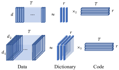
Figure 3. Illustration of NMF (top) and NTF (bottom). $m$-mode tensors are observed $n$ times. One seeks $m$ loading matrices as well as a code matrix that gives an approximate decomposition of all data.

The constrained tensor factorization problem (139) falls under the framework of BCD in (3), since the objective function $f$ in (139) is convex in each loading matrix $U^{(i)}$ for $i=1,\dots,m$. Indeed, BCD is a popular approach for both NMF and NTF problems [35]. Namely, when we apply BCD (3) for (139), each block update amounts to solving a quadratic problem under convex constraint. BCD for (139) is known as the form of alternating least squares (ALS). For NMF, ALS (or vanilla BCD in (3)) is known to converge to stationary points [28]. However, for NTF with $m\geq 3$ modes, global convergence to stationary points of ALS is not guaranteed in general [34] and requires some additional regularity conditions [8, 28]. Using our general framework of BMM-DR, we propose the following iterative algorithms for constrained tensor factorization: For each $n\geq 1$ and $i=1,\dots,m$,

(142) BMM-DR for CTF

(143) $$\begin{cases}\mathbf{A}\leftarrow\operatorname{\texttt{Out}}(U^{(1)}_{n-1},\dots,U^{(i-1)}_{n-1},U^{(i+1)}_{n-1},\dots,U^{(m-1)}_{n-1})\in\mathbb{R}^{(I_{1}\times\cdots\times I_{i-1}\times I_{i+1}\times\cdots\times I_{m})\times R}\\ B\leftarrow\textup{unfold}(\mathbf{A},m)\in\mathbb{R}^{(I_{1}\cdots I_{i-1}I_{i+1}\cdots I_{m})\times R}\\ g_{n}^{(i)}(U)\leftarrow\textup{Majorizing surrogate of $f_{n}^{(i)}(U):=\lVert\textup{unfold}(\mathbf{X},i)-BU^{T}\rVert_{F}^{2}+\lambda_{i}\lVert U\rVert_{1}$}\\ U_{n}^{(i)}\in\operatorname*{arg\,min}_{U\in\Theta^{(i)},\,\lVert U-U_{n-1}^{(i)}\rVert_{F}\leq r_{n}}\,g_{n}^{(i)}(U),\end{cases}$$

where $\textup{unfold}(\cdot,i)$ denotes the mode-$i$ tensor unfolding (see [34]) and $r_{n}\in[0,\infty]$ for $n\geq 1$ denotes radius of trust-region. The iterate (142) specializes in various tensor factorization algorithms depending on the choice of the surrogate $g_{n}^{(i)}$. Namely, first, there are four ALS-type algorithms:

1. (ALS)  $g_{n}^{(i)}=f_{n}^{(i)}$, $r_{n}\equiv\infty$

2. (ALS with DR)  $g_{n}^{(i)}=f_{n}^{(i)}$, $\sum_{n=1}^{\infty}r_{n}=\infty,\sum_{n=1}^{\infty}r_{n}^{2}<\infty$.

3. (ALS with PR)  $g_{n}^{(i)}(U)=f_{n}^{(i)}(U)+\frac{\rho}{2}\lVert U-U_{n-1}^{(i)}\rVert_{F}^{2}$, $\rho>0$, and $r_{n}\equiv\infty$.

4. (ALS with DR+PR)  $g_{n}^{(i)}(U)=f_{n}^{(i)}(U)+\frac{\rho}{2}\lVert U-U_{n-1}^{(i)}\rVert_{F}^{2}$, $\rho>0$, $\sum_{n=1}^{\infty}r_{n}=\infty$, and $\sum_{n=1}^{\infty}r_{n}^{2}<\infty$.

Next, specialize (139) into NCPD, where $\Theta^{(i)}=\mathbb{R}^{I_{i}\times R}_{\geq 0}$ and $\lambda_{i}=0$ for $i=1,\dots m$. There are two MU-type algorithms for NCPD, which can be derived similarly as in the NMF case (see Sec. 5.1):

1. (MU) $g_{n}^{(i)}=g_{n}$ in (118) with $\delta=\rho=0$, $H=U^{T}$, $X=\textup{unfold}(\mathbf{X},i)$, and $W_{n}=B$. This yields the following factor update:

   (144) $$(U_{n+1}^{(i)})^{T}\leftarrow U_{n}^{(i)}\odot(B^{T}\textup{unfold}(\mathbf{X},i))\oslash(B^{T}BU_{n}^{(i)}).$$

2. (MUR)  $g_{n}^{(i)}=g_{n}$ in (118) with $\delta,\rho>0$, $H=U^{T}$, $X=\textup{unfold}(\mathbf{X},i)$, and $W_{n}=B$. This yields the following factor update:

   (145) $$\begin{cases}\tilde{U}\leftarrow U_{n}^{(i)}\lor\delta\\ (U_{n+1}^{(i)})^{T}\leftarrow\tilde{U}\odot\left((B^{T}\textup{unfold}(\mathbf{X},i))+\rho\tilde{U}^{T}\right)\oslash((B^{T}B+\rho\mathbf{I})\tilde{U}).\end{cases}$$

For many instances of BMM-DR for CTF listed above, we can apply our general result (Theorem 2.1) to deduce their convergence and complexity. Unfortunately, Theorem 2.1 does not cover the case when the objective is non-differentiable, so we may need to assume zero $L_{1}$-regularization in (139). Furthermore, in order to guarantee asymptotic convergence to stationary points and iteration complexity as stated in Theorem 2.1, we need to assume that either diminishing radius or majorization with a quadratic gap is used. This rules out the vanilla ALS (a) for general CTF and MU (e) for NCPD. The following corollary holds for all the other options listed above.

Corollary 5.2 (Convergence of BMM-DR for CTF).

Suppose no sparsity regularizaiton is assumed ($\lambda_{1}=\dots=\lambda_{m}=0$) in (139). Let $\boldsymbol{\theta}_{n}:=[U^{(1)}_{n},\dots,U^{(m)}_{n}]$, $n\geq 0$ be generated by (142) with one of the options (b), (c), (d) (for general convex constraints on factor matrices) or (f) (for NCPD). Then (i)-(iii) of Theorem 2.1 holds for $(\boldsymbol{\theta}_{n})_{n\geq 0}$.

Remark 5.3.

In recent joint work with Strohmeier and Needell [48], the first author has developed an online version of constrained tensor factorization and convergence analysis under mild assumptions. The technique of using diminishing radius was first introduced in the reference to encourage the stability of iterates in an online setting.

5.3. Block Projected Gradient Descent

In the introduction, we discussed that the block projected gradient descent (BPGD) (6) is a special instance of BMM where prox-linear surrogates are exactly minimized over convex constraint sets. Therefore, our general result (Theorem 2.1) implies that the BPGD algorithm (6) converges asymptotically to the stationary points (not only Nash equilibrium) and also has iteration complexity of $\widetilde{O}(\varepsilon^{-2})$, under the hypothesis of Theorem 2.1. See Corollary 5.4.

Corollary 5.4 (Complexity of Block PGD).

Let $(\boldsymbol{\theta}_{n})_{n\geq 0}$ be generated by the block projected gradient descent updates (6). Suppose A1 and A2 hold, where the convex constraint sets $\Theta^{(i)}$ are not necessarily bounded. Further, assume that the stepsize $1/\lambda$ is sufficiently small. Then (i)-(iii) of Theorem 2.1 holds for $(\boldsymbol{\theta}_{n})_{n\geq 0}$. In particular, the iteration complexity for smooth nonconvex objectives with convex constraints is $\tilde{O}(\varepsilon^{-2})$.

To the best of our knowledge, Corollary 5.4 is the first complexity result of block PGD for smooth nonconvex objectives. In [79], under a mild condition, it was shown that the above algorithm converges asymptotically to a Nash equilibrium (a weaker notion than stationary points) and also a local rate of convergence under the Kurdyka-Łojasiewicz condition is established. Also, the convergence of BPGD in terms of the function values for convex objectives with complexity $\tilde{O}(\varepsilon^{-1})$ is known [12]. Recently, iteration complexity of $\tilde{O}(\varepsilon^{-2})$ of block gradient descent on compact Riemannian manifolds has been obtained [61, 26]. These results concern constraints given by compact Riemannian manifold without boundary, which applies neither for the unconstrained Euclidean space (for being unbounded) nor compactly constrained Euclidean space (for having boundary).

5.4. Expectation Maximization (EM) Algorithm [23]

The well-known Expectation Maximization (EM) algorithm is another concrete example of the MM algorithm. Let $\boldsymbol{\theta}$ be the parameters to be estimated and $w$ be the observations. Denote $p(w\mid\boldsymbol{\theta})$ as the conditional probability of $w$ given $\boldsymbol{\theta}$. Let $z$ be a random vector representing some hidden variables. The maximum likelihood estimation problem w.r.t $\boldsymbol{\theta}$ constrained in a convex set $\boldsymbol{\Theta}$ is formulated as the following,

(146) $$\min_{\boldsymbol{\theta}\in\boldsymbol{\Theta}}\left(f(\boldsymbol{\theta}):=\;-\ln{p(w\mid\boldsymbol{\theta})}\right).$$

The proximal EM algorithm is an iterative algorithm as follows:

(147) $$\textbf{Proximal EM}\quad\begin{cases}\textup{{E-step}:}\;g_{n}(\boldsymbol{\theta}):=-\mathbb{E}_{z|w,\boldsymbol{\theta}_{n-1}}\left[\ln{p(w,z\mid\boldsymbol{\theta})}\right]+\mathbb{E}_{z\mid w,\boldsymbol{\theta}_{n-1}}\left[\ln p\left(z\mid w,\boldsymbol{\theta}_{n-1}\right)\right],\\ \textup{{proximal M-step}: }\boldsymbol{\theta}_{n}=\operatorname*{arg\,min}_{\boldsymbol{\theta}\in\boldsymbol{\Theta}}\left(g_{n}(\boldsymbol{\theta})+\frac{\rho}{2}\lVert\boldsymbol{\theta}-\boldsymbol{\theta}_{n-1}\rVert^{2}\right),\end{cases}$$

where $\rho\geq 0$ is the proximal regularization parameter. If $\rho=0$, then (147) reduces to the standard EM algorithm. Note that we allow the parameter $\boldsymbol{\theta}$ can have additional convex constraint $\boldsymbol{\Theta}$ (e.g., $\boldsymbol{\theta}$ could be the covariance matrix of a multivariate Gaussian variable with independent coordinates. Then $\boldsymbol{\Theta}$ is the set of diagonal matrices of nonnegative diagonal entries).

EM and its proximal version in (147) are classical examples of the MM algorithm. To see this, note that

(148) $$-\ln p(w\mid\boldsymbol{\theta}) \overset{(a)}{=}-\ln\,\mathbb{E}_{z\mid\boldsymbol{\theta}}\left[p(w\mid z,\boldsymbol{\theta})\right]$$

(149) $$=-\ln\,\mathbb{E}_{z\mid\boldsymbol{\theta}}\left[\frac{p\left(z\mid w,\boldsymbol{\theta}_{n-1}\right)p(w\mid z,\boldsymbol{\theta})}{p\left(z\mid w,\boldsymbol{\theta}_{n-1}\right)}\right]$$

(150) $$\overset{(b)}{=}-\ln\,\mathbb{E}_{z\mid w,\boldsymbol{\theta}_{n-1}}\left[\frac{p(z\mid\boldsymbol{\theta})p(w\mid z,\boldsymbol{\theta})}{p\left(z\mid w,\boldsymbol{\theta}_{n-1}\right)}\right]$$

(151) $$\overset{(c)}{\leq}-\mathbb{E}_{z\mid w,\boldsymbol{\theta}_{n-1}}\ln\left[\frac{p(z\mid\boldsymbol{\theta})p(w\mid z,\boldsymbol{\theta})}{p\left(z\mid w,\boldsymbol{\theta}_{n-1}\right)}\right]$$

(152) $$=-\mathbb{E}_{z\mid w,\boldsymbol{\theta}_{n-1}}\ln p(w,z\mid\boldsymbol{\theta})+\mathbb{E}_{z\mid w,\boldsymbol{\theta}_{n-1}}\ln p\left(z\mid w,\boldsymbol{\theta}_{n-1}\right)$$

(153) $$=g_{n}(\boldsymbol{\theta}),$$

where (a) is due to an iterated expectation, (b) is due to Bayes’ rule, and (c) follows from Jensen’s inequality. Hence $g_{n}$ is a majorizing surrogate of $\boldsymbol{\theta}\mapsto-\ln p(w\mid\boldsymbol{\theta})$. Furthermore, $g_{n}(\boldsymbol{\theta}_{n-1})=f(\boldsymbol{\theta}_{n-1})$. Hence we conclude that the proximal EM algorithm (as well as the EM) is a special case of the MM algorithm.

Under some assumption on the likelihood function, we can apply our general result for BMM (Theorem 2.1) to derive convergence and complexity results for the proximal EM algorithm, as stated in the following corollary.

Corollary 5.5 (Convergence of proximal EM).

Let $(\boldsymbol{\theta}_{n})_{n\geq 0}$ denote the (possibly inexact) output of the proximal EM algorithm (147) with arbitrary initialization $\boldsymbol{\theta}_{0}\in\boldsymbol{\Theta}$. Suppose the following hold:

(A1-EM)

A2 holds for the log-likelihood function in (146).

(A2-EM)

The gap in the Jensen’s inequality in (151) is upper bounded by $\frac{L_{h}}{2}\lVert\boldsymbol{\theta}-\boldsymbol{\theta}_{n-1}\rVert^{2}$ for some constant $L_{h}>0$.

(A3-EM)

The optimality gaps of the M-step are summable (see A4).

(A4-EM)

$g_{n}$ in (147) has $L_{g}$-Lipschitz continuous gradients for some $L_{g}>0$ and $\rho>L_{g}$.

Then (i)-(iii) of Theorem 2.1 for $r_{n}\equiv\infty$ hold for the proximal EM.

We also remark that one can consider EM with diminishing radius (instead of proximal regularization) and apply Theorem 2.1 under suitable assumptions that warrant the hypothesis of this theorem. Furthermore, one could also extend the EM algorithm to a multi-block case, which would make it a special instance of the BMM algorithm [62, 43]. We can also consider the block EM with either proximal regularization or diminishing radius, and obtain a similar corollary as above. We omit the detailed discussion.

6. Experimental Validation

6.1. Comparison between MU and MUR for NMF

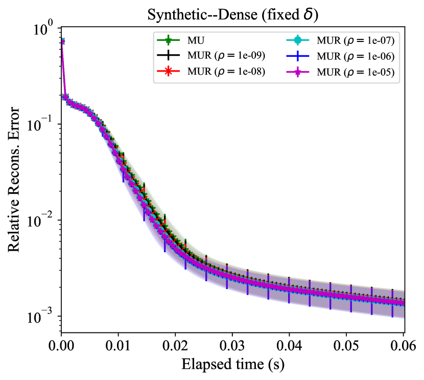
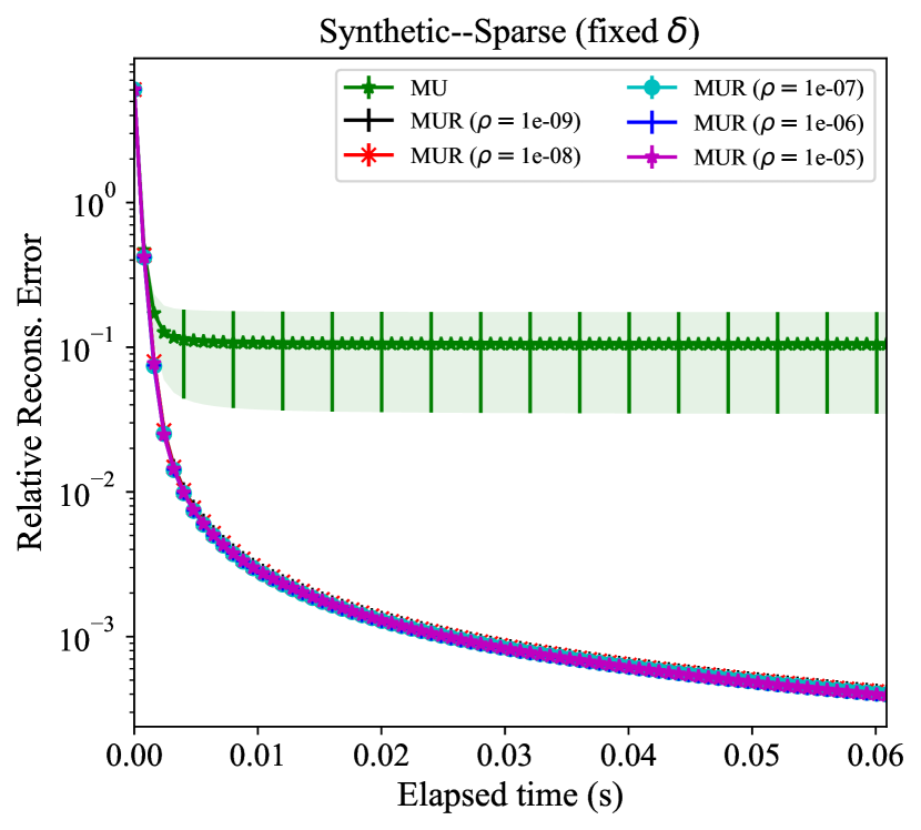
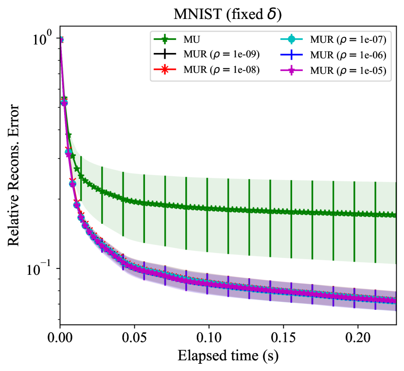
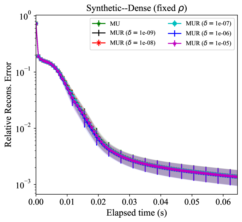
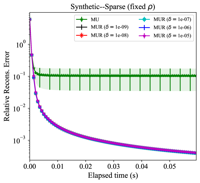
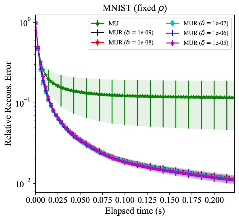
Figure 4. Comparison of the performance of MUR for the nonnegative matrix factorization (NMF) problem against MU. For MUR in the first (second) row, $\delta$ ($\rho$) is fixed as $10^{-8}$. The number of columns of loading matrices is set to be $r=2$ for synthetic data and $r=15$ for MNIST data. The average relative reconstruction error with standard deviation is shown by the solid lines and shaded regions of respective colors.

In this section, we compare the performance of our MUR (115) for the task of NMF (113) against the original MU (114). We consider both synthetic data and real-world data: (1) Synthetic data $\mathbf{X}_{\textup{synth}}\in\mathbb{R}^{100\times 50}_{\geq 0}$ equals $WH$ where $W\in\mathbb{R}^{100\times 2}_{\geq 0}$ and $H\in\mathbb{R}^{2\times 50}_{\geq 0}$ are generated by sampling each entry uniformly and independently from the unit interval $[0,1]$; (2) Sparse synthetic data $\mathbf{X}_{\textup{synth-sp}}\in\mathbb{R}^{100\times 50}_{\geq 0}$ is generated in the same way as $\mathbf{X}_{\textup{synth}}$ but with sparsity $0.2$, i.e. only $20\%$ of the entries are non-zero; (3) MNIST data $\mathbf{X}_{\textup{MNIST}}\in\mathbb{R}^{28\times 28}_{\geq 0}$ (height $\times$ width) is one figure randomly sampled from the MNIST data set [22].

In numerical experiments, we use MU and MUR to learn nonnegative matrices $W\in\mathbb{R}^{100\times 2}_{\geq 0}$ and $H\in\mathbb{R}^{2\times 50}_{\geq 0}$ with synthetic data, and $W\in\mathbb{R}^{28\times 15}_{\geq 0}$ and $H\in\mathbb{R}^{15\times 28}_{\geq 0}$ with MNIST data. MU and MUR with various threshold parameters $\delta$ and regularization parameter $\rho$ are run $100$ times in each experiment with random initial data. The average relative reconstruction error with standard deviation is computed and shown in Figure 4 with solid lines and shaded regions. As shown in Figure 4, in the synthetic data case without the sparsity feature, MU and MUR show similar convergence speeds. In the sparse data case, for both synthetic and MNIST data, MUR with various parameters significantly outperforms MU. One could find clues of underlying reason from the updates of MU in Section 5.1. In fact, from (133), the step size of gradient descent updates involves $H$ and $W$ in both the denominator and numerator, whose elements could possibly be zero especially when the data is sparse. A zero numerator of the step size results in no change during updates, while a zero denominator would lead to blow-up issues. These challenges contribute to the comparatively poorer performance of MU when compared to MUR. MUR overcomes the issues with the help of parameters $\rho$ and $\delta$, as discussed in detail in Section 5.1.

6.2. Nonnegative CP-decomposition

In this section, we compare the performance of our proposed BMM-DR algorithm (Algorithm 1, implemented as (142) for NCPD) and MUR (142)((f)) for the task of NCPD (139) (with no $L_{1}$-regularization, i.e., $\lambda_{1}=\lambda_{2}=\lambda_{3}=0$) against two most popular approaches in practice: 1) The vanilla BCD (3) (known as Alternating Least Squares for NCPD); and 2) Multiplicative Update (MU) (see [67]). Recall that we recover the standard ALS from (142) by setting $r_{n}=\infty$ for $n\geq 1$. We consider one synthetic and one real-world tensor data as follow:

1. $\mathbf{X}_{\text{synth}}\in\mathbb{R}_{\geq 0}^{100\times 50\times 30}$ equals $\operatorname{\texttt{Out}}(V_{1},V_{2},V_{3})$, where the true loading matrices $V_{1}\in\mathbb{R}_{\geq 0}^{100\times 2}$, $V_{2}\in\mathbb{R}_{\geq 0}^{50\times 2}$, and $V_{3}\in\mathbb{R}_{\geq 0}^{30\times 2}$ are generated by sampling each of their entries uniformly and independently from the unit interval $[0,1]$.

2. $\mathbf{X}_{\textup{Cifar10}}\in\mathbb{R}_{\geq 0}^{1000\times 32\times 32\times 3}$ $(\textup{samples}\times\textup{height}\times\textup{width}\times\textup{RGB})$ is $1000$ samples randomly sampled from the Cifar 10 dataset [37]. The four modes correspond to samples, height, width, and RGB channels, in order. Since the last dimension is only $3$ by its nature, we need to transform it into a $3$-tensor to better facilitate the algorithms. Namely, we obtain a 3-D slice by selecting the data along the RGB channels, specifically using the values from the first channel (R). This process resulted in a new $3$-tensor $\mathbf{X}_{\textup{Cifar10-R}}\in\mathbb{R}_{\geq 0}^{1000\times 32\times 32}$ $(\textup{samples}\times\textup{height}\times\textup{width})$, representing the grayscale version of the original images.

For each data tensor $\mathbf{X}$ of shape $I_{1}\times I_{2}\times I_{3}$, we used the aforementioned algorithms to learn three loading matrices $U_{i}\in\mathbb{R}^{I_{i}\times R}$ for $i=1,2,3$. We set the number of columns $R=2$ for synthetic data and $R=10$ for the Cifar10 dataset. Each algorithm is run 10 times with independent random initial data in each case, and the plot shows the average relative reconstruction error (the square root of $f_{\textup{CTF}}$ in (139) divided by $\lVert\mathbf{X}\rVert_{F}$) together with their standard deviation in shades. The results are shown in Figure 5.

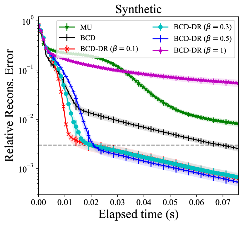
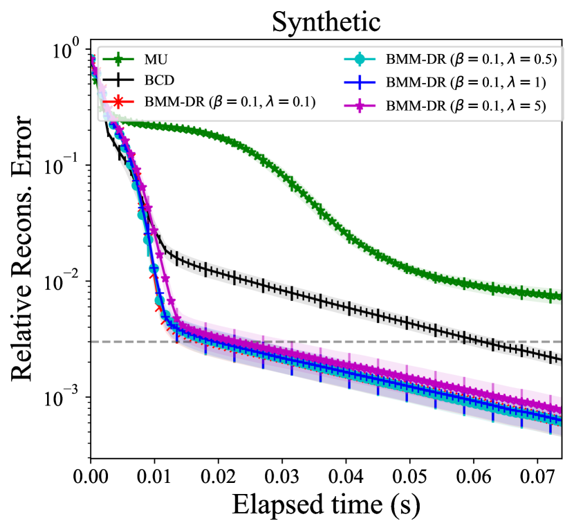
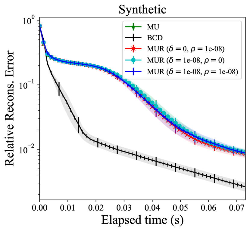
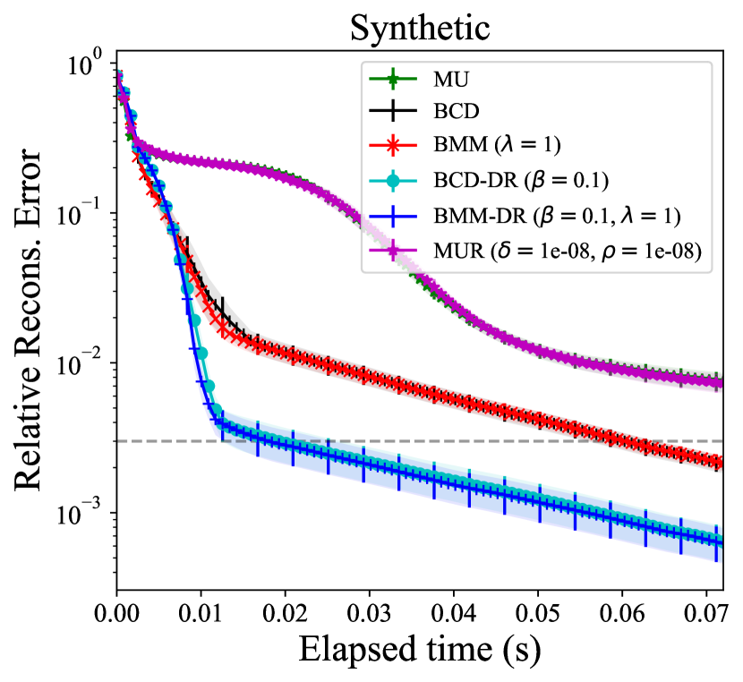
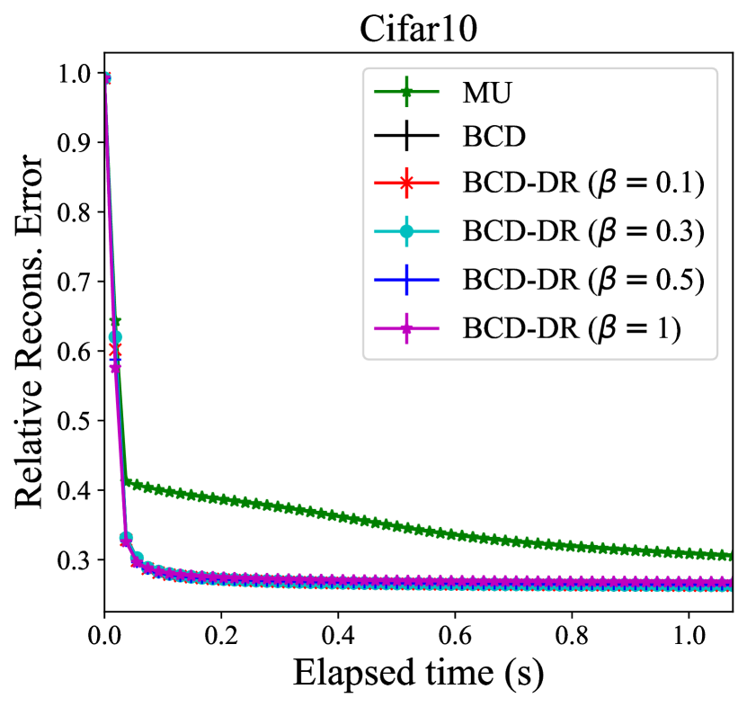
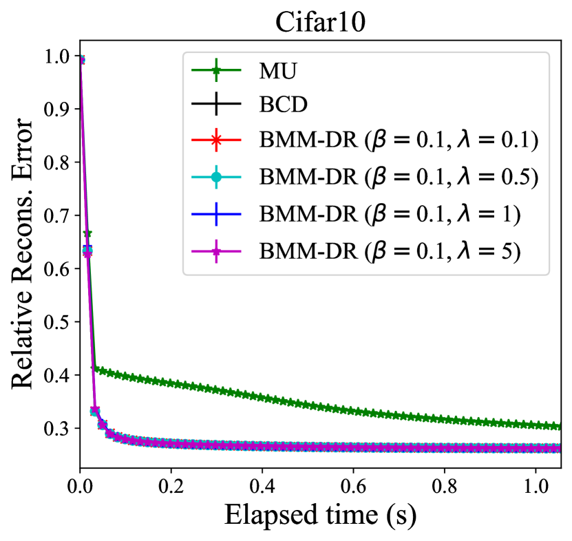
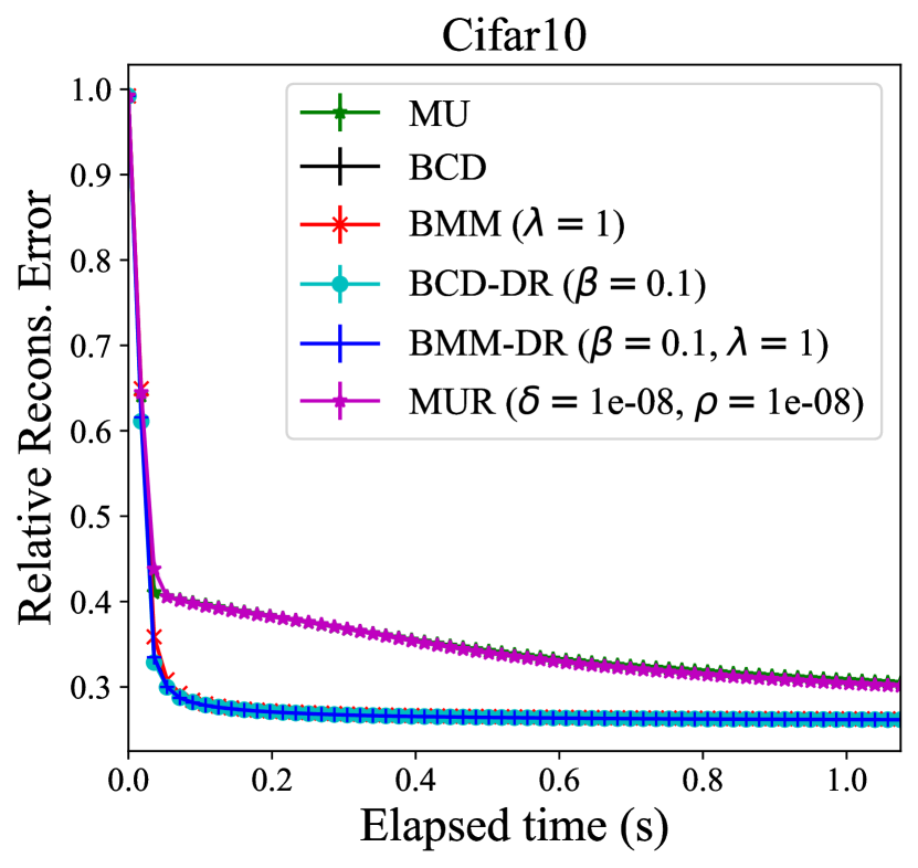
Figure 5. Comparison of the performance of BMM-DR (Algorithm 1) and MUR against BCD and MU for the nonnegative CP-decomposition (NCPD) problem. BCD is implmented as (142)((a)) with $r_{n}=\infty$ for $n\geq 1$ (equivalent to Alternating Least Sqaures). BCD-DR is implemented as (142)((b)) with $c^{\prime}=\lVert\mathbf{X}\rVert_{F}/(1.5\times 10^{5})$ for synthetic data and $c^{\prime}=\lVert\mathbf{X}\rVert_{F}/(3\times 10^{5})$ for Cifar10 data ($\mathbf{X}$ denoting the data tensor) and weights $r_{n}=n^{-\beta}/\log n$ for $n\geq 1$ for both. BMM ((c)) is implemented with a proximal regularizer with parameter $\lambda$. BMM-DR ((d)) is implemented on top of BMM with diminishing radius with parameter $\beta=0.1$ and same $c^{\prime}$ as BCD-DR. MU and MUR are implemented as ((e)) and ((f)), respectively. The average relative reconstruction error with standard deviation is shown by the solid lines and shaded regions of respective colors.

In the experiments, BCD-DR is implemented as (142). Using the same notations as in (142), denote the marginal loss function as

(154) $$f_{n}^{(i)}(U^{(i)})=\left\|\operatorname{unfold}(X,i)-B\left(U^{(i)}\right)^{T}\right\|_{F}^{2}.$$

Instead of directly minimizing $f_{n}^{(i)}$, BMM-DR minimizes a surrogate function $g_{n}^{(i)}$ in each iteration with

(155) $$g_{n}^{(i)}(U^{(i)}):=f_{n}^{(i)}(U^{(i)})+\lambda_{n}\|U^{(i)}-U^{(i)}_{n-1}\|_{F}^{2}=\left\|\operatorname{unfold}(X,i)-B\left(U^{(i)}\right)^{T}\right\|_{F}^{2}+\lambda_{n}\|U^{(i)}-U^{(i)}_{n-1}\|_{F}^{2}.$$

Then the updates of BMM-DR can be written as

(156) $$U_{n}^{(i)}\in\operatorname*{arg\,min}_{U\in\Theta^{(i)},\,\lVert U-U_{n-1}^{(i)}\rVert\leq r_{n}}\,\lVert\textup{unfold}(\mathbf{X},i)-B(U^{(i)})^{T}\rVert_{F}^{2}+\lambda_{n}\|U^{(i)}-U^{(i)}_{n-1}\|_{F}^{2}.$$

We take all the regularization parameters $\lambda_{n}$ to be constant in our numerical examples, i.e. $\lambda_{n}=\lambda>0$.

For synthetic data, as shown in Figure 5, BCD-DR with proper diminishing radius parameters $\beta$ and $c^{\prime}$ is significantly faster than MU and also the standard vanilla BCD in terms of elapsed time. The choice of $c^{\prime}$ is important to achieve the best performance of BCD-DR. Here we take $c^{\prime}=\lVert\mathbf{X}\rVert_{F}/(1.5\times 10^{5})$ where $\mathbf{X}$ denote the synthetic data tensor, and $1.5\times 10^{5}$ is the number of elements in the tensor. Similarly, a proper value of $\beta$ is also crucial for fast convergence, here as shown in Figure 5, BCD-DR with $\beta=0.1$ attains its best performance. In the case of BMM-DR algorithms, we set $\beta$ to $0.1$ and conduct tests using varying values of parameter $\lambda$. Remarkably, BMM-DR consistently outperforms both MU and the standard vanilla BCD in terms of elapsed time across all tested $\lambda$ values. As for the comparison of MU and MUR, they show similar convergence speed since the tensor data is dense (detailed discussion in Section 6.1).

For the Cifar 10 data set, the same experiments are conducted with $c^{\prime}=\lVert\mathbf{X}\rVert_{F}/(3\times 10^{5})$. All BCD-DR and BMM-DR outperform MU in terms of elapsed time and demonstrate a comparable convergence rate to the vanilla BCD. Diminishing radius (DR) does not accelerate the convergence as in the synthetic data case, due to the difference of the observed tensor data. In the synthetic data case, the tensor data is generated by loading matrices, so one is able to recover the loading matrices with a small relative reconstruction error. In fact, the acceleration from DR becomes significant when the relative reconstruction error is of order $10^{-2}$. However, decomposing real-world tensor to loading matrices with such a small relative reconstruction error may not be possible, since an approximate solution of (138) with such a small error may not exist. Hence, the acceleration from DR is not observed in the Cifar 10 data set case.

6.3. CANDECOMP/PARAFAC (CP) dictionary learning

In this section, we study the performance of BMM-DR (Algorithm 1) for the task of general unconstrained CP-dictionary learning (139) (with no $L_{1}$-regularization, i.e., $\lambda_{1}=\lambda_{2}=\lambda_{3}=0$), namely, $\Theta^{(i)}=\mathbb{R}^{I_{i}\times R}$ for $i=1,2,3$. We compare its performance with vanilla BCD, which is also known as Alternating Least Square (ALS). For BMM algorithms, we still use the proximal surrogates (155).

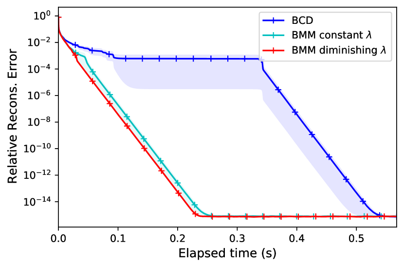
(a) Synthetic data 1

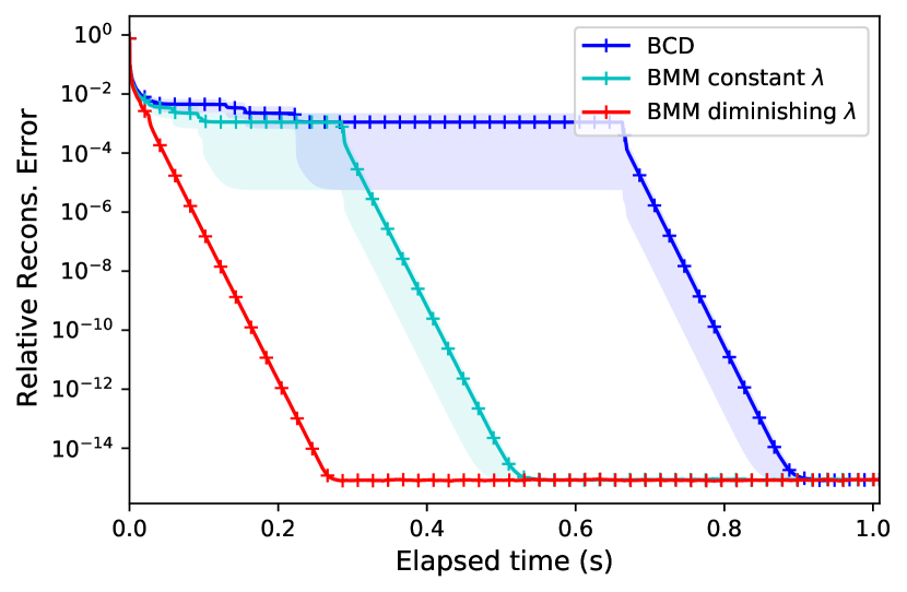
(b) Synthetic data 2

Figure 6. Comparison of the performance of BMM (Algorithm 1) for the CP-decomposition (CPD) problem against BCD (known as ALS). (A) and (B) are two examples of different synthetic data. The average relative reconstruction error with standard deviation is shown by the solid lines and shaded regions of respective colors.

For unconstrained CP dictionary learning problem, we have access to the closed form solution of minimizing $f_{n}^{(i)}$ (154) (for BCD) and $g_{n}^{(i)}$ (155) (for BMM). In fact, recall for $A\in\mathbb{R}^{M\times R}$, $B\in\mathbb{R}^{M\times N}$ and $X\in\mathbb{R}^{R\times N}$, an exact least square solution is as following,

(157) $$(A^{T}A)^{\dagger}A^{T}B\in\operatorname*{arg\,min}_{X\in\mathbb{R}^{R\times N}}\|AX-B\|^{2}_{F},$$

where $\dagger$ denotes the Pseudoinverse. This gives an exact closed-form solution to the subproblem of minimizing $f_{n}^{(i)}$. Also, note one could rewrite the proximal regularized least square problem as follows,

(158) $$\min_{X\in\mathbb{R}^{R\times N}}\|AX-B\|^{2}+\lambda\|X-X_{k}\|^{2}=\min_{X\in\mathbb{R}^{R\times N}}\left\|\left(\begin{array}[]{c}A\\ \sqrt{\lambda}I\end{array}\right)X-\left(\begin{array}[]{c}B\\ \sqrt{\lambda}X_{k}\end{array}\right)\right\|^{2},$$

where $X_{k}\in\mathbb{R}^{R\times N}$ denotes the previous iterate. Hence, one could get the exact closed-form solution to the subproblem of minimizing $g_{n}^{(i)}$ in the same way. This closed-form solution allows BCD and BMM to converge efficiently and accurately to the true solution in the synthetic data case. Below we provide some numerical examples.

For numerical experiments, we generate synthetic tensor data $X\in\mathbb{R}^{30\times 20\times 10}$ as $\operatorname{\texttt{Out}}(U^{(1)},U^{(2)},U^{(3)})$, where the true loading matrices $U^{(1)}\in\mathbb{R}^{30\times 3}$, $U^{(2)}\in\mathbb{R}^{20\times 3}$, and $U^{(3)}\in\mathbb{R}^{10\times 3}$ are generated by sampling each of their entries independently from standard normal distribution. Vanilla BCD, BMM with constant $\lambda_{n}=0.1$, and BMM with diminishing $\lambda_{n}=0.1\times 0.5^{n}$ as suggested in [52] are applied to find loading matrices $U^{(1)},U^{(2)},U^{(3)}$ with $R=3$ columns. We run each algorithm 100 times from the independent random initialization and then compute the averaged relative error. Two synthetic data examples are shown in Figure 6 (A) and (B). In both examples, BMM significantly outperforms BCD in terms of elapsed time.

References

- ABRS [10] Hédy Attouch, Jérôme Bolte, Patrick Redont, and Antoine Soubeyran, Proximal alternating minimization and projection methods for nonconvex problems: An approach based on the kurdyka-łojasiewicz inequality, Mathematics of operations research 35 (2010), no. 2, 438–457.
- AEB [06] Michal Aharon, Michael Elad, and Alfred Bruckstein, K-svd: An algorithm for designing overcomplete dictionaries for sparse representation, IEEE Transactions on signal processing 54 (2006), no. 11, 4311–4322.
- AL [23] Ahmet Alacaoglu and Hanbaek Lyu, Convergence of stochastic first-order methods with dependent data for constrained nonconvex optimization, International Conference on Machine Learning (2023).
- BB [05] Michael W Berry and Murray Browne, Email surveillance using non-negative matrix factorization, Computational & Mathematical Organization Theory 11 (2005), no. 3, 249–264.
- BBL+ [07] Michael W Berry, Murray Browne, Amy N Langville, V Paul Pauca, and Robert J Plemmons, Algorithms and applications for approximate nonnegative matrix factorization, Computational statistics & data analysis 52 (2007), no. 1, 155–173.
- BCN [18] Léon Bottou, Frank E Curtis, and Jorge Nocedal, Optimization methods for large-scale machine learning, Siam Review 60 (2018), no. 2, 223–311.
- Bec [17] Amir Beck, First-order methods in optimization, SIAM, 2017.
- Ber [97] Dimitri P Bertsekas, Nonlinear programming, Journal of the Operational Research Society 48 (1997), no. 3, 334–334.
- Ber [99] by same author, Nonlinear programming, Athena scientific Belmont, 1999.
- BMB+ [15] Rostyslav Boutchko, Debasis Mitra, Suzanne L Baker, William J Jagust, and Grant T Gullberg, Clustering-initiated factor analysis application for tissue classification in dynamic brain positron emission tomography, Journal of Cerebral Blood Flow & Metabolism 35 (2015), no. 7, 1104–1111.
- Bot [10] Léon Bottou, Large-scale machine learning with stochastic gradient descent, Proceedings of COMPSTAT’2010, Springer, 2010, pp. 177–186.
- BT [13] Amir Beck and Luba Tetruashvili, On the convergence of block coordinate descent type methods, SIAM journal on Optimization 23 (2013), no. 4, 2037–2060.
- BT [15] Dimitri Bertsekas and John Tsitsiklis, Parallel and distributed computation: numerical methods, Athena Scientific, 2015.
- CC [70] J Douglas Carroll and Jih-Jie Chang, Analysis of individual differences in multidimensional scaling via an n-way generalization of “eckart-young” decomposition, Psychometrika 35 (1970), no. 3, 283–319.
- CGT [10] Coralia Cartis, Nicholas IM Gould, and Ph L Toint, On the complexity of steepest descent, newton’s and regularized newton’s methods for nonconvex unconstrained optimization problems, Siam journal on optimization 20 (2010), no. 6, 2833–2852.
- CM [09] Olivier Cappé and Eric Moulines, On-line expectation–maximization algorithm for latent data models, Journal of the Royal Statistical Society Series B: Statistical Methodology 71 (2009), no. 3, 593–613.
- CP [11] Patrick L Combettes and Jean-Christophe Pesquet, Proximal splitting methods in signal processing, Fixed-point algorithms for inverse problems in science and engineering (2011), 185–212.
- CSWD [23] Xufeng Cai, Chaobing Song, Stephen Wright, and Jelena Diakonikolas, Cyclic block coordinate descent with variance reduction for composite nonconvex optimization, International Conference on Machine Learning, PMLR, 2023, pp. 3469–3494.
- CWS+ [11] Yang Chen, Xiao Wang, Cong Shi, Eng Keong Lua, Xiaoming Fu, Beixing Deng, and Xing Li, Phoenix: A weight-based network coordinate system using matrix factorization, IEEE Transactions on Network and Service Management 8 (2011), no. 4, 334–347.
- DD [19] Damek Davis and Dmitriy Drusvyatskiy, Stochastic model-based minimization of weakly convex functions, SIAM Journal on Optimization 29 (2019), no. 1, 207–239.
- DDFG [10] Ingrid Daubechies, Ronald DeVore, Massimo Fornasier, and C Sinan Güntürk, Iteratively reweighted least squares minimization for sparse recovery, Communications on Pure and Applied Mathematics: A Journal Issued by the Courant Institute of Mathematical Sciences 63 (2010), no. 1, 1–38.
- Den [12] Li Deng, The mnist database of handwritten digit images for machine learning research, IEEE Signal Processing Magazine 29 (2012), no. 6, 141–142.
- DLR [77] Arthur P Dempster, Nan M Laird, and Donald B Rubin, Maximum likelihood from incomplete data via the em algorithm, Journal of the royal statistical society: series B (methodological) 39 (1977), no. 1, 1–22.
- EA [06] Michael Elad and Michal Aharon, Image denoising via sparse and redundant representations over learned dictionaries, IEEE Transactions on Image processing 15 (2006), no. 12, 3736–3745.
- EAH [99] Kjersti Engan, Sven Ole Aase, and John Hakon Husoy, Frame based signal compression using method of optimal directions (mod), ISCAS’99. Proceedings of the 1999 IEEE International Symposium on Circuits and Systems VLSI (Cat. No. 99CH36349), vol. 4, IEEE, 1999, pp. 1–4.
- GHN [23] David H Gutman and Nam Ho-Nguyen, Coordinate descent without coordinates: Tangent subspace descent on riemannian manifolds, Mathematics of Operations Research 48 (2023), no. 1, 127–159.
- GS [99] Luigi Grippof and Marco Sciandrone, Globally convergent block-coordinate techniques for unconstrained optimization, Optimization methods and software 10 (1999), no. 4, 587–637.
- GS [00] Luigi Grippo and Marco Sciandrone, On the convergence of the block nonlinear gauss–seidel method under convex constraints, Operations research letters 26 (2000), no. 3, 127–136.
- GZ [05] Edward F Gonzalez and Yin Zhang, Accelerating the lee-seung algorithm for nonnegative matrix factorization, Tech. report, 2005.
- H+ [57] Clifford Hildreth et al., A quadratic programming procedure, Naval research logistics quarterly 4 (1957), no. 1, 79–85.
- HRLP [15] Mingyi Hong, Meisam Razaviyayn, Zhi-Quan Luo, and Jong-Shi Pang, A unified algorithmic framework for block-structured optimization involving big data: With applications in machine learning and signal processing, IEEE Signal Processing Magazine 33 (2015), no. 1, 57–77.
- HWRL [17] Mingyi Hong, Xiangfeng Wang, Meisam Razaviyayn, and Zhi-Quan Luo, Iteration complexity analysis of block coordinate descent methods, Mathematical Programming 163 (2017), 85–114.
- JH [91] Christian Jutten and Jeanny Herault, Blind separation of sources, part i: An adaptive algorithm based on neuromimetic architecture, Signal processing 24 (1991), no. 1, 1–10.
- KB [09] Tamara G Kolda and Brett W Bader, Tensor decompositions and applications, SIAM review 51 (2009), no. 3, 455–500.
- KHP [14] Jingu Kim, Yunlong He, and Haesun Park, Algorithms for nonnegative matrix and tensor factorizations: A unified view based on block coordinate descent framework, Journal of Global Optimization 58 (2014), no. 2, 285–319.
- KL [23] Dohyun Kwon and Hanbaek Lyu, Complexity of block coordinate descent with proximal regularization and applications to wasserstein cp-dictionary learning, International Conference on Machine Learning (2023).
- Kri [09] Alex Krizhevsky, Learning multiple layers of features from tiny images, Tech. report, 2009.
- KW [18] Koulik Khamaru and Martin Wainwright, Convergence guarantees for a class of non-convex and non-smooth optimization problems, International Conference on Machine Learning, PMLR, 2018, pp. 2601–2610.
- LHK [05] Kuang-Chih Lee, Jeffrey Ho, and David J Kriegman, Acquiring linear subspaces for face recognition under variable lighting, IEEE Transactions on pattern analysis and machine intelligence 27 (2005), no. 5, 684–698.
- LHY [00] Kenneth Lange, David R Hunter, and Ilsoon Yang, Optimization transfer using surrogate objective functions, Journal of computational and graphical statistics 9 (2000), no. 1, 1–20.
- [41] Chih-Jen Lin, On the convergence of multiplicative update algorithms for nonnegative matrix factorization, IEEE Transactions on Neural Networks 18 (2007), no. 6, 1589–1596.
- [42] by same author, Projected gradient methods for nonnegative matrix factorization, Neural computation 19 (2007), no. 10, 2756–2779.
- LLM [18] Sharon X Lee, Kaleb L Leemaqz, and Geoffrey J McLachlan, A block em algorithm for multivariate skew normal and skew -mixture models, IEEE transactions on neural networks and learning systems 29 (2018), no. 11, 5581–5591.
- LMWY [12] Ji Liu, Przemyslaw Musialski, Peter Wonka, and Jieping Ye, Tensor completion for estimating missing values in visual data, IEEE transactions on pattern analysis and machine intelligence 35 (2012), no. 1, 208–220.
- LS [99] Daniel D Lee and H Sebastian Seung, Learning the parts of objects by non-negative matrix factorization, Nature 401 (1999), no. 6755, 788.
- LS [00] Michael S Lewicki and Terrence J Sejnowski, Learning overcomplete representations, Neural computation 12 (2000), no. 2, 337–365.
- LS [01] Daniel D Lee and H Sebastian Seung, Algorithms for non-negative matrix factorization, Advances in neural information processing systems, 2001, pp. 556–562.
- LSN [22] Hanbaek Lyu, Christopher Strohmeier, and Deanna Needell, Online nonnegative cp-dictionary learning for markovian data, The Journal of Machine Learning Research 23 (2022), no. 1, 6630–6679.
- LT [92] Zhi-Quan Luo and Paul Tseng, On the convergence of the coordinate descent method for convex differentiable minimization, Journal of Optimization Theory and Applications 72 (1992), no. 1, 7–35.
- LX [17] Zhaosong Lu and Lin Xiao, A randomized nonmonotone block proximal gradient method for a class of structured nonlinear programming, SIAM Journal on Numerical Analysis 55 (2017), no. 6, 2930–2955.
- MBPS [09] Julien Mairal, Francis Bach, Jean Ponce, and Guillermo Sapiro, Online dictionary learning for sparse coding, Proceedings of the 26th annual international conference on machine learning, 2009, pp. 689–696.
- NDLK [08] Carmeliza Navasca, Lieven De Lathauwer, and Stefan Kindermann, Swamp reducing technique for tensor decomposition, 2008 16th European Signal Processing Conference, IEEE, 2008, pp. 1–5.
- Nes [98] Yurii Nesterov, Introductory lectures on convex programming volume i: Basic course, Lecture notes 3 (1998), no. 4, 5.
- Nes [12] Yu Nesterov, Efficiency of coordinate descent methods on huge-scale optimization problems, SIAM Journal on Optimization 22 (2012), no. 2, 341–362.
- Nes [13] by same author, Gradient methods for minimizing composite functions, Mathematical programming 140 (2013), no. 1, 125–161.
- NH [98] Radford M Neal and Geoffrey E Hinton, A view of the em algorithm that justifies incremental, sparse, and other variants, Learning in graphical models, Springer, 1998, pp. 355–368.
- NKLR+ [10] Masahiro Nakano, Hirokazu Kameoka, Jonathan Le Roux, Yu Kitano, Nobutaka Ono, and Shigeki Sagayama, Convergence-guaranteed multiplicative algorithms for nonnegative matrix factorization with -divergence, 2010 IEEE International Workshop on Machine Learning for Signal Processing, IEEE, 2010, pp. 283–288.
- OF [97] Bruno A Olshausen and David J Field, Sparse coding with an overcomplete basis set: A strategy employed by v1?, Vision research 37 (1997), no. 23, 3311–3325.
- Pow [73] Michael JD Powell, On search directions for minimization algorithms, Mathematical programming 4 (1973), no. 1, 193–201.
- PPP [06] V Paul Pauca, Jon Piper, and Robert J Plemmons, Nonnegative matrix factorization for spectral data analysis, Linear algebra and its applications 416 (2006), no. 1, 29–47.
- PV [23] Liangzu Peng and René Vidal, Block coordinate descent on smooth manifolds, arXiv preprint arXiv:2305.14744 (2023).
- RHL [13] Meisam Razaviyayn, Mingyi Hong, and Zhi-Quan Luo, A unified convergence analysis of block successive minimization methods for nonsmooth optimization, SIAM Journal on Optimization 23 (2013), no. 2, 1126–1153.
- RLH [20] Sirisha Rambhatla, Xingguo Li, and Jarvis Haupt, Provable online cp/parafac decomposition of a structured tensor via dictionary learning, arXiv preprint arXiv:2006.16442 (2020).
- RPZ+ [18] Bin Ren, Laurent Pueyo, Guangtun Ben Zhu, John Debes, and Gaspard Duchêne, Non-negative matrix factorization: robust extraction of extended structures, The Astrophysical Journal 852 (2018), no. 2, 104.
- RW [09] R Tyrrell Rockafellar and Roger J-B Wets, Variational analysis, vol. 317, Springer Science & Business Media, 2009.
- SGH [02] Arkadiusz Sitek, Grant T Gullberg, and Ronald H Huesman, Correction for ambiguous solutions in factor analysis using a penalized least squares objective, IEEE transactions on medical imaging 21 (2002), no. 3, 216–225.
- SH [05] Amnon Shashua and Tamir Hazan, Non-negative tensor factorization with applications to statistics and computer vision, Proceedings of the 22nd international conference on Machine learning, ACM, 2005, pp. 792–799.
- SH [15] Ruoyu Sun and Mingyi Hong, Improved iteration complexity bounds of cyclic block coordinate descent for convex problems, Advances in Neural Information Processing Systems 28 (2015).
- SLLC [17] Will Wei Sun, Junwei Lu, Han Liu, and Guang Cheng, Provable sparse tensor decomposition, Journal of the Royal Statistical Society: Series B (Statistical Methodology) 3 (2017), no. 79, 899–916.
- SS [73] RWH Sargent and DJ Sebastian, On the convergence of sequential minimization algorithms, Journal of Optimization Theory and Applications 12 (1973), no. 6, 567–575.
- SSY [18] Tao Sun, Yuejiao Sun, and Wotao Yin, On markov chain gradient descent, Advances in Neural Information Processing Systems, 2018, pp. 9896–9905.
- ST [13] Ankan Saha and Ambuj Tewari, On the nonasymptotic convergence of cyclic coordinate descent methods, SIAM Journal on Optimization 23 (2013), no. 1, 576–601.
- TH [14] Norikazu Takahashi and Ryota Hibi, Global convergence of modified multiplicative updates for nonnegative matrix factorization, Computational Optimization and Applications 57 (2014), 417–440.
- TN [12] Leo Taslaman and Björn Nilsson, A framework for regularized non-negative matrix factorization, with application to the analysis of gene expression data, PloS one 7 (2012), no. 11, e46331.
- Tse [91] Paul Tseng, Decomposition algorithm for convex differentiable minimization, Journal of Optimization Theory and Applications 70 (1991), no. 1, 109–135.
- TY [09] Paul Tseng and Sangwoon Yun, A coordinate gradient descent method for nonsmooth separable minimization, Mathematical Programming 117 (2009), 387–423.
- Wri [15] Stephen J Wright, Coordinate descent algorithms, Mathematical Programming 151 (2015), no. 1, 3–34.
- WWB [19] Rachel Ward, Xiaoxia Wu, and Leon Bottou, Adagrad stepsizes: Sharp convergence over nonconvex landscapes, International Conference on Machine Learning, PMLR, 2019, pp. 6677–6686.
- XY [13] Yangyang Xu and Wotao Yin, A block coordinate descent method for regularized multiconvex optimization with applications to nonnegative tensor factorization and completion, SIAM Journal on imaging sciences 6 (2013), no. 3, 1758–1789.
- XYY+ [19] Yi Xu, Zhuoning Yuan, Sen Yang, Rong Jin, and Tianbao Yang, On the convergence of (stochastic) gradient descent with extrapolation for non-convex optimization, arXiv preprint arXiv:1901.10682 (2019).
- YR [03] Alan L Yuille and Anand Rangarajan, The concave-convex procedure, Neural computation 15 (2003), no. 4, 915–936.
- Zaf [09] Stefanos Zafeiriou, Algorithms for nonnegative tensor factorization, Tensors in Image Processing and Computer Vision, Springer, 2009, pp. 105–124.
- ZT [17] Renbo Zhao and Vincent YF Tan, A unified convergence analysis of the multiplicative update algorithm for regularized nonnegative matrix factorization, IEEE Transactions on Signal Processing 66 (2017), no. 1, 129–138.
- ZVB+ [16] Shuo Zhou, Nguyen Xuan Vinh, James Bailey, Yunzhe Jia, and Ian Davidson, Accelerating online cp decompositions for higher order tensors, Proceedings of the 22nd ACM SIGKDD International Conference on Knowledge Discovery and Data Mining, 2016, pp. 1375–1384.