Adaptive Local Bayesian Optimization
Over Multiple Discrete Variables

Abstract

In the machine learning algorithms, the choice of the hyperparameter is often an art more than a science, requiring labor-intensive search with expert experience. Therefore, automation on hyperparameter optimization to exclude human intervention is a great appeal, especially for the black-box functions. Recently, there have been increasing demands of solving such concealed tasks for better generalization, though the task-dependent issue is not easy to solve. The Black-Box Optimization challenge (NeurIPS 2020) required competitors to build a robust black-box optimizer across different domains of standard machine learning problems. This paper describes the approach of team KAIST OSI in a step-wise manner, which outperforms the baseline algorithms by up to +20.39%. We first strengthen the local Bayesian search under the concept of region reliability. Then, we design a combinatorial kernel for a Gaussian process kernel. In a similar vein, we combine the methodology of Bayesian and multi-armed bandit (MAB) approach to select the values with the consideration of the variable types; the real and integer variables are with Bayesian, while the boolean and categorical variables are with MAB. Empirical evaluations demonstrate that our method outperforms the existing methods across different tasks.

1 Introduction

Bayesian optimization (BO) [12] has long been known for its sample efficiency without any need for derivative information, and thus it is widely adopted in black-box optimization problems. In each iteration, BO constructs a posterior distribution of the unknown objective (i.e., surrogate model) based on the observations and then selects an expectedly promising point for the next evaluation (i.e., acquisition function). It is particularly known for its performance in hyperparameter optimization within heavily restricted evaluation budgets [13]. However, recent literature has addressed that existing works lack consideration on the case when configuration consists of discrete variables [11, 9]. To deal with this issue, a stream of work has appeared with variations of standard surrogate models and acquisition functions to reflect the different features that discrete variables inherently possess adequately.

The Black-Box Optimization (BBO) challenge hosted by NeurIPS 2020 asked the participants to provide an optimizer capable of tuning a wide range of machine learning problems on real-world datasets . Since most of the current studies do not consider the existence of discrete variables, we mainly focused on mitigating the issue of mixed variables. We have applied approaches from different angles to handle the issue.

Our solution can be broken down into four steps: (1) a quick hyperparameter tuning of the baseline model TuRBO (Trust Region BO), which by itself effectively leads to a global optimum by using a collection of simultaneous local optimization with independent probabilistic models  [6] (Subsection 2.1), (2) adaptive region partitioning with support vector machine (SVM) (Subsection 2.2), (3) combination of different kernels for different types of variables (Subsection 2.3), and (4) replacement of qualitative variables (i.e. categorical and boolean) by bandit approach based on Thompson sampling (Subsection 2.4). Figure 1 illustrates an outline of our algorithm.

1.1 Challenge Overview

The BBO challenge provided the benchmark package (bayesmark) , which supports the local experiments based on the real-world datasets with different objectives and models. The leaderboard score is determined by the performance score on held-out objective functions within the 640 seconds of time limit exclusively on generating suggestions (16 iterations with batch size of 8). The challenge platform provided both the validity and computed score on the validation problem set until the final submission. The official score is decided by the test problem set.

2 Approaches

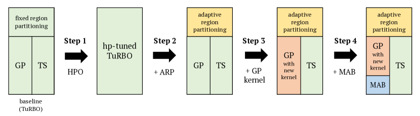
Figure 1: An overview of our algorithm; The baseline consists of local Bayesian modeling which composes a standard Gaussian Process (GP) with matèrn kernel as a surrogate model and Thompson sampling (TS) as an acquisition function. After hyperparameter tuning (Step 1), we compensated for its region partitioning by making it adaptive to different tasks (Step 2). Then, for the discrete variables, we introduced a mixture of different kernels for GP (Step 3) and combined MAB for regeneration of qualitative variables (Step 4).

2.1 Baseline: TuRBO

Through the score comparison of the baseline optimizers on the validation set, we chose the TuRBO as our starting point, which ranked the highest performance above all (Table 1).

Table 1: A preliminary survey of the baseline algorithms on the validation problem set.

Algorithm	Random Search	HyperOpt [2]	SkOpt [7]	SkOpt2 [7]	Opentuner [1]	TuRBO [6]	PySOT [5]
Score	80.224	88.127	91.867	91.932	84.801	95.307	93.902

TuRBO runs multiple bayesian optimizations by incorporating separate subregions which they coined as trust regions. Then, it sorts out the next best candidate by implicit Thompson sampling. The algorithm takes standard models for its components where Gaussian process (GP) is selected for the surrogate model and Thompson sampling (TS) to acquire the next point.

In detail, it first makes a hyper-rectangle centered by the current best observation with its initial length equally set for all dimensions. The Sobol sequence [3] is sampled from the bounded region, and then it computes their likelihood to select the promising candidates. If the candidate turns out to be the new best point, it perceives success and doubles the length of corresponding trust region. Whereas for all the other cases, it recognizes as a failure and halves them all. If the rescaled length reaches the certain threshold, the trust region restarts from scratch.

We improved the performance of TuRBO through a brief, manual search on hyperparameters that are related to trust region. First, we tuned the minimum length of trust region which directly infers the restarting criterion. In consequence, we settled down with a higher value of minimum length than the default hence the algorithm would behave as more of a quick decision maker for restart (Table 2). Also, further tuning were made on the number of trust regions for parallel search. TuRBO with multiple trust regions takes the advantage of sampling from separate local models. However, as it consumes a lot of evaluation to initiate individual regions, which is a burden in our constrained setting, we used a single trust region for the subsequent experiments.

Table 2: Validation scores according to different minimum length; $2^{-7}$ is the default setting.

Minimum Length	$2^{-1}$	$2^{-2}$	$2^{-3}$	$2^{-4}$	$2^{-5}$	$2^{-6}$	$2^{-7}$	$2^{-16}$
Score	93.694	95.186	95.906	95.473	95.379	95.501	95.307	93.902

2.2 Adaptive Region Partitioning (ARP)

Despite the remarkable performance of TuRBO in its quick and efficient optimization, it has several noteworthy weaknesses. First, it owns a stiff criterion on constructing the trust region; i.e., it bounds the local region with fixed rules regardless of the problem setting. Different combinations of objectives and datasets form different landscapes for optimization, hence taking it into account is a better policy. Another weakness is that TuRBO restarts from scratch; therefore time consumption to initiate the new phase may be fatal in a limited budget.

To alleviate these drawbacks, we proposed a simple yet effective method, called ARP (Adaptive Region Partitioning) with a hint from Wang et al. [15]. ARP is a method of adding a classifier as a helper tool not only to reshape the constructed trust region but also to restart within a promising region (2(d)). ARP is activated after stacking a sufficient amount of observations. First, at each iteration, the observations are labeled into two groups - good region and bad region - based on the evaluation values by k-means clustering (2(b)). Then, SVM learns the decision boundary through synthetic labels (2(c)), and as a consequence, it can be used to partition within the current trust region so that candidates are extracted from the selected (good) region (2(d)). Also in the restart phase, random samples are created within the selected region using the pretrained classifier. Then, even after a number of restarts, the newly initiated trust region can be built upon a reliable subregion instead of the whole search space.

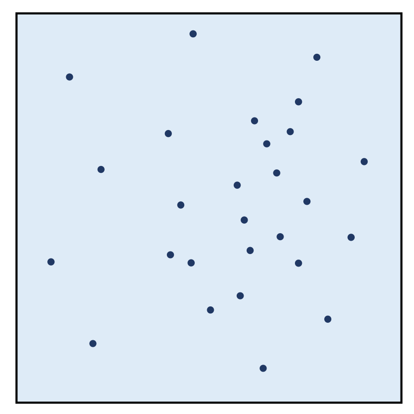
(a)

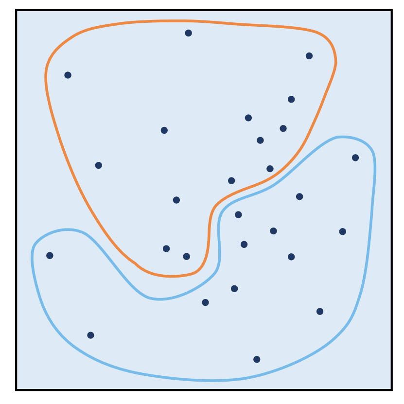
(b)

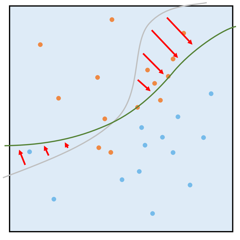
(c)

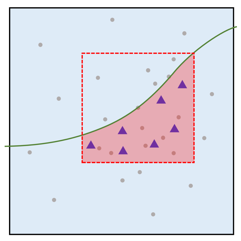
(d)

Figure 2: An overview of ARP; (2(a)) the dots represent the evaluated observations in the search space, (2(b)) first, we produce labels with k-means clustering, (2(c)) then, we retrain the classifier to learn the new boundary, (2(d)) the trained classifier is used to partition the trust region so that the next sampling is generated within the selected region. Here we select the region that includes the current best point. The clustering and classifier training are held under global observations.

Our key differentiation from Wang et al. [15] is that our algorithm utilizes all the data points to train the classifier, i.e. the partition always consider the entire region. In Wang et al. [15], they bifurcate the search space into a tree structure and then train the classifier only with the points within the selected local region. While their strategy may be effective when sufficient amount of budget is given, it would be a bottleneck under the consideration of the limited iterations of the challenge. In this respect, the entire data is employed to learn the region partitioning in our implementation.

2.3 A Mixture of Different GP Kernels

In this subsection, we introduced a new design of kernel to remedy the absence of the consideration of discrete variables. Recent studies have suggested a solution of mixing multiple kernels [8, 11]. For instance, a summation of additive kernels [8] and a combination of sum and product of two separate kernels for continuous inputs and categorical inputs [11] are discussed. From the insight of the previous works [8, 11], we adopted a novel kernel as follows:

$${k}_{M}(\mathbf{x},\mathbf{x^{{}^{\prime}}})=\frac{2^{1-\nu}}{\Gamma{(\nu)}}(\sqrt{2\nu}d){K_{\nu}}(\sqrt{2\nu}d),\quad{k}_{L}(\mathbf{y},\mathbf{y^{{}^{\prime}}})={v}\mathbf{y^{T}}\mathbf{y^{{}^{\prime}}},\quad{k}_{I}(\mathbf{z},\mathbf{z^{{}^{\prime}}})=\mathbbm{1}(\mathbf{z},\mathbf{z^{{}^{\prime}}})$$ (1)

$${k}(\mathbf{h},\mathbf{h^{{}^{\prime}}})=(1-\lambda)({k}_{M}(\mathbf{x},\mathbf{x^{{}^{\prime}}})+{k}_{L}(\mathbf{y},\mathbf{y^{{}^{\prime}}})+{k}_{I}(\mathbf{z},\mathbf{z^{{}^{\prime}}}))+\lambda{k}_{M}(\mathbf{x},\mathbf{x^{{}^{\prime}}}){k}_{L}(\mathbf{y},\mathbf{y^{{}^{\prime}}}){k}_{I}(\mathbf{z},\mathbf{z^{{}^{\prime}}})$$ (2)

where $h$ is an input that decomposed into $x$, $y$, and $z$, each respectively matching to continuous, integer, and categorical / boolean variables, $d$ indicates the Euclidean distance between $x$ and $x^{{}^{\prime}}$, $\lambda$ is the balancing parameter between kernels, $\nu$ serves as the smoothness parameter for matèrn kernel, $v$ represents the signal variance parameter for linear kernel, and $\mathbbm{1}(z,z^{{}^{\prime}})=1$ if $z=z^{{}^{\prime}}$ and otherwise 0. For the implementation, we fixed the value as 2.5 for $\nu$ and 1 for $v$, which generally worked well in our local experiments.

Separating kernels would detect different inherent features of each type, where the specific type of kernel is chosen based on the empirical result on the validation set. As shown in Eq. (1) and (2), these kernels are integrated by linear combination of product and sum to learn the correlation between types of variables.

2.4 Multi-Armed Bandits on Qualitative Variables

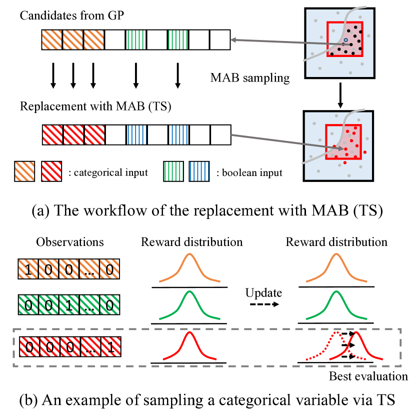
Figure 3: An overview of bandit.

After extracting candidates from the GP (Subsection 2.3), the values of categorical and boolean variables are replaced with the samples from Thompson sampling (TS). We empirically found out that TuRBO’s local search strategy led to repeated bounding around same points, thereby particularly providing excessive exploitation on certain types of variables. In detail, TuRBO often seems to select the same values for the qualitative variables repeatedly during one phase of trust region search. TuRBO’s shrinking policy on failure intensifies this lack of exploration; as a result, it would inevitably spend redundant time in limited space where the bounded region may be worthless for further search.

To compensate the insufficient exploration of local search, we add an alternative for the aforementioned variables that are particularly under-explored. In specific, we chose MAB as a substitute to generate categorical and boolean variables while leaving float and integer with GP. Although we made a partial replacement with MAB, the GP with our constructed kernel enables the algorithm to learn the correlation between different variables. For integer variable, despite its discreteness, we exclude it from applying MAB since it rather acts as a continuous variable in the sense that both are quantitative  [14, 10, 4]. If the candidate turns out to be the best evaluation, each $\alpha$ parameter in the beta distribution of the corresponding arms increases  (Figure 3 (b)) as a reward.

3 Conclusion and Future works

Algorithm	Baseline	+ Tuning	+ ARP	+ Mixture Kernel & Bandit
Score	95.307	95.906	96.298	96.580

Table 3: The validation scores of the algorithm; the preceding additions are included in each steps

Along with the described steps, we have recorded the leaderboard scores, which clearly show that each addition enhanced the baseline to a certain extent (Table 3). Regarding the final evaluation on the test problem set, our method rated 90.875 as an official score, ranking 8th in the final leaderboard.

We have mainly focused on treating the discrete variables, which distinctively possess different characteristics comparing to continuous variables. Our approach numerically proved its improvement comparing to the baseline methods (see Table 4 in Appendix B). Despite its superiority, there are still lacks on the theoretical analysis about the regret bound of MAB and the convergence guarantee of our designed kernel. As future work, a theoretical analysis of the remarkable performance of local search can be expected.

Appendix A Challenge Overview

The training datasets can be found in https://scikit-learn.org/stable/datasets/index.html#toy-datasets (Figure 4). The leaderboard is determined using the optimization performance on held-out (hidden) objective functions, where the optimzier must run without human intervention.

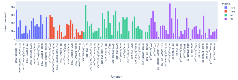
Figure 4: A result of the TuRBO [6] on the local experiments in the benchmark package. Under the given scikit-learn datasets, a black-box optimizer is evaluated with various combinations of machine learning models (e.g. MLP, linear, kNN) and metrics (e.g. mae, mse, acc, nll).

Appendix B Improvement of Our Algorithm on Validation Set

Table 4: A preliminary survey of the baseline algorithms on the validation dataset. Improvement was calculated based on equation $\frac{(S_{o}-S_{b})}{S_{b}}$ where $S_{o}$ and $S_{b}$ indicates our score and baseline score, respectively.

Algorithm	Random Search	HyperOpt [2]	SkOpt [7]	SkOpt2 [7]	Opentuner [1]	TuRBO [6]	PySOT [5]	Ours
Score	80.224	88.127	91.867	91.932	84.801	95.307	93.902	96.580
Improvement	+ 20.39%	+ 9.59 %	+ 5.13 %	+ 5.06 %	+ 13.89 %	+ 1.34 %	+ 2.85 %	-

References

- [1] Jason Ansel, Shoaib Kamil, Kalyan Veeramachaneni, Jonathan Ragan-Kelley, Jeffrey Bosboom, Una-May O’Reilly, and Saman Amarasinghe. Opentuner: An extensible framework for program autotuning. In International Conference on Parallel Architectures and Compilation Techniques, Edmonton, Canada, Aug 2014.
- [2] James Bergstra, Daniel Yamins, and David Cox. Making a science of model search: Hyperparameter optimization in hundreds of dimensions for vision architectures. In International conference on machine learning, pages 115–123. PMLR, 2013.
- [3] Sebastian Burhenne, Dirk Jacob, and Gregor Henze. Sampling based on sobol’ sequences for monte carlo techniques applied to building simulations. pages 1816–1823, 01 2011.
- [4] Erik Daxberger, Anastasia Makarova, Matteo Turchetta, and Andreas Krause. Mixed-variable bayesian optimization. arXiv preprint arXiv:1907.01329, 2019.
- [5] David Eriksson, David Bindel, and Christine A Shoemaker. pysot and poap: An event-driven asynchronous framework for surrogate optimization. arXiv preprint arXiv:1908.00420, 2019.
- [6] David Eriksson, Michael Pearce, Jacob Gardner, Ryan D Turner, and Matthias Poloczek. Scalable global optimization via local bayesian optimization. In Advances in Neural Information Processing Systems, pages 5496–5507, 2019.
- [7] Tim Head, MechCoder, Gilles Louppe, Iaroslav Shcherbatyi, fcharras, Zé Vinícius, cmmalone, Christopher Schröder, nel215, Nuno Campos, Todd Young, Stefano Cereda, Thomas Fan, Justus Schwabedal, Hvass-Labs, Mikhail Pak, SoManyUsernamesTaken, Fred Callaway, Loïc Estève, Lilian Besson, Peter M. Landwehr, Pavel Komarov, Mehdi Cherti, Kejia (KJ) Shi, Karlson Pfannschmidt, Fabian Linzberger, Christophe Cauet, Anna Gut, Andreas Mueller, and Alexander Fabisch. scikit-optimize/scikit-optimize: v0.5.1 - re- release, February 2018.
- [8] Kirthevasan Kandasamy, Jeff Schneider, and Barnabás Póczos. High dimensional bayesian optimisation and bandits via additive models. In International conference on machine learning, pages 295–304, 2015.
- [9] Henry Moss, David Leslie, Daniel Beck, Javier Gonzalez, and Paul Rayson. Boss: Bayesian optimization over string spaces. Advances in neural information processing systems, 33, 2020.
- [10] Julien Pelamatti, Loïc Brevault, Mathieu Balesdent, El-Ghazali Talbi, and Yannick Guerin. Overview and comparison of gaussian process-based surrogate models for mixed continuous and discrete variables: Application on aerospace design problems. In High-Performance Simulation-Based Optimization, pages 189–224. Springer, 2020.
- [11] Binxin Ru, Ahsan S Alvi, Vu Nguyen, Michael A Osborne, and Stephen J Roberts. Bayesian optimisation over multiple continuous and categorical inputs. arXiv preprint arXiv:1906.08878, 2019.
- [12] Bobak Shahriari, Kevin Swersky, Ziyu Wang, Ryan P Adams, and Nando De Freitas. Taking the human out of the loop: A review of bayesian optimization. Proceedings of the IEEE, 104(1):148–175, 2015.
- [13] Jasper Snoek, Hugo Larochelle, and Ryan P Adams. Practical bayesian optimization of machine learning algorithms. In Advances in neural information processing systems, pages 2951–2959, 2012.
- [14] Laura P Swiler, Patricia D Hough, Peter Qian, Xu Xu, Curtis Storlie, and Herbert Lee. Surrogate models for mixed discrete-continuous variables. In Constraint Programming and Decision Making, pages 181–202. Springer, 2014.
- [15] Linnan Wang, Rodrigo Fonseca, and Yuandong Tian. Learning search space partition for black-box optimization using monte carlo tree search. NeurIPS, 2020.