Dynamic structure factors of a strongly interacting Fermi superfluid near an orbital Feshbach resonance across the phase transition from BCS to Sarma superfluid

Abstract

We theoretically investigate dynamic structure factors of a strongly interacting Fermi superfluid near an orbital Feshbach resonance with random phase approximation approach at zero temperature, and find their dynamical characters across the phase transition from a balanced conventional Bardeen-Cooper-Schrieffer superfluid to a polarized Sarma superfluid by continuously varying the chemical potential difference of two spin components. In a BEC-like regime of the Fermi superfluid, dynamic structure factors can help distinguish the in-phase ground state from the out-of-phase metastable state by the relative location of molecular excitation and Leggett mode, or the minimum energy to break a Cooper pair. In the phase transition from BCS to Sarma superfluid, we find the dynamic structure factor of Sarma superfluid has its own specific gapless excitation at a small transferred momentum where the collective phonon excitation acquires a finite width, and also a relatively strong atomic excitation at a large transferred momentum, because of the existence of unpaired Fermi atoms. Our results can be used to differentiate Sarma superfluid from BCS superfluid.

I Introduction

Interacting quantum many-body system is always a central research field in physics, and contains many interesting but also challenging problems. As a many-body physical quantity, the density-density dynamic structure factor, i.e., the Fourier transformation of density-density correlation function, contains rich information about the dynamical excitation of the system pitaevskiibook . At a low transferred momentum regime, one can observe many kinds of collective excitations, while molecular and atomic excitation can be seen at a large transferred momentum. Besides the spectrum of the system, dynamic structure factors also display the weight distribution of both Fermi atoms and Cooper-pairs according to the width and strength of excitation peak. From both the spectrum and weight distribution we can understand rich many-body properties, like the pair condensation and transition temperature lingham2014 , Tan’s contact parameter kuhnle2011 ; hoinka2013 , etc,. Generally the experimental measurement of many-body physical quantities is a quite difficult task, luckily a two-photon Bragg scattering technique can be able to measure dynamic structure factors at an almost full regime of transferred momentum veeravalli2008 ; hoinka2017 ; hoinka2012 ; brunello2001 .

The accumulation of interacting many particles can form lots of quantum matter states, i.e. Fulde-Ferrell-Larkin-Ovchinnikov (FFLO) phases fulde1964 ; larkin1964 , Sarma superfluid sarma1963 , topological superfluid zhang2008 etc,. The search and distinguishment of new matter states in different materials or microscopic particles system are interesting and important jobs. The BCS-type Fermi superfluid is a conventional superfluid state, where two Fermi atoms with the same amplitude of momentum but unlike direction and spin can form a Cooper pair with zero momentum of center of mass. It is usually the ground state of many superconductors or Fermi superfluid. A Sarma superfluid is a possible candidate ground state for a spin-polarized Fermi superfluid. Having gapless fermionic excitations, this state can be viewed as a phase separation state in momentum space: some fermions pair and form a superfluid, while other unpaired atoms just occupy in certain regions of momentum space bounded by gapless Fermi surfaces.

In the context of two-component spin-1/2 Fermi atomic gas at the famous BEC-BCS crossover, Sarma superfluid can only be stable on the BEC side of the crossover. It may also be stabilized by considering a multiband structure he2009 , which experimentally can be realized with alkali-earth-metal atoms (such as Sr) or alkali-earth-metal-like atoms (i.e. Yb), where there are two electrons outside the atoms. In this case the usual Magnetic Feshbach resonance fails to tune the effective interacting strength since their zero magnetic moment difference, but a pioneering work by R. Zhang et al theoretical proposed an alternative mechanism of orbital Feshbach resonance (OFR) for ¹⁷³Yb zhang2015 . In Fermi gases of ¹⁷³Yb, the long-lived metastable electric orbital state ${}^{3}P_{0}$ (denoted as $\left|e\sigma\right\rangle$ where $\sigma=\uparrow,\downarrow$ stands for the two internal nuclear spin states) can be chosen, together with the ground orbital state ${}^{1}S_{0}$ ($\left|g\sigma\right\rangle$) . In fact this forms a four-component Fermi system, where a pair of atoms can be described by using the singlet ($-$) and triplet ($+$) basis in the absence of external Zeeman field,

$$\left|\pm\right\rangle=\frac{1}{2}\left(\left|ge\right\rangle\pm\left|eg\right\rangle\right)\otimes\left(\left|\uparrow\downarrow\right\rangle\mp\left|\downarrow\uparrow\right\rangle\right),$$ (1)

or by a usual two-channel basis in the presence of the Zeeman field

$$\left|o\right\rangle=\frac{1}{\sqrt{2}}\left(\left|-\right\rangle+\left|+\right\rangle\right)=\frac{1}{\sqrt{2}}\left(\left|g\uparrow,e\downarrow\right\rangle-\left|e\downarrow,g\uparrow\right\rangle\right),$$ (2)

$$\left|c\right\rangle=\frac{1}{\sqrt{2}}\left(\left|-\right\rangle-\left|+\right\rangle\right)=\frac{1}{\sqrt{2}}\left(\left|g\downarrow,e\uparrow\right\rangle-\left|e\uparrow,g\downarrow\right\rangle\right),$$ (3)

where $o$ and $c$ are short for open and close channel, respectively. The interparticle interaction is described by a $s$-wave scattering length, namely the singlet scattering length $a_{-}$ and the triplet one $a_{+}$. Because of a shallow bound state (related to a large $a_{+}\simeq 1900a_{0}$, where $a_{0}$ is the Bohr radius) caused by the interorbital (nuclear) spin-exchange interaction, the small difference in the nuclear Landé factor between different orbital states allows the tunability of scattering length in the open channel through an external magnetic fieldzhang2015 . The existence of the predicted OFR has been confirmed soon experimentally pagano2015 ; hofer2015 . More fascinatingly, OFR is a narrow resonance due to the significant closed-channel fraction xu2016 , and a two-channel mode he2015 is really necessary to provide a right description. In the two-channel system, the exchange interaction between two channels varies significantly the stability mechanism of the pairing state, and makes Sarma state, which is always unstable in single-channel system, can be a stable ground state he2009 once a nonzero interband exchange interaction and a large asymmetry between the two bands are existent. In our recent work, a superfluid phase transition from a balanced conventional Bardeen-Cooper-Schrieffer superfluid to a polarized Sarma superfluid in a strongly interacting Fermi superfluid near an orbital Feshbach resonance has been reported zou2018 .

It is of great interest to explore the many-body physical eigenstates of OFR, and investigate their rich dynamics. The existence of two order parameters in OFR has opened the possibility of observing the long-sought massive Leggett mode resulted from the fluctuation of the relative phase of the two order parameters, which can be observed in both BCS and Sarma superfluid leggett1966 ; blumberg2007 ; lin2012 ; bittner2015 ; klimin2019 . So it is interesting to study all dynamics of OFR , and find their specific characters in different matter states, from which to research possibility to distinguish different many-body eigenstates, or different ground states of OFR by an experimental observable many-body physical quantity. Following this idea, we would like to investigate the dynamic structure factor across the phase transition process from BCS superfluid to Sarma superfluid in OFR, and find their own specific dynamical characters which may service as fingerprints of different matter states.

This paper is organized as follows. In the next section, we will use the language of Green’s function to introduce the microscopic model of a three-dimensional Fermi superfluid near OFR with both spin-balanced and spin-polarized population , outline the mean-field approximation and how to calculate response function with random phase approximation, and give the results of dynamic structure factor of BCS superfluid in Sec. III, and the results of Sarma superfluid in Sec. IV. In Sec. V and VI, we will give our conclusions and acknowledgement, respectively.

II Mean-field theory

II.1 Model Hamiltonian

The spin-population imbalanced Fermi gases near orbital Feshbach resonance can be described by a two-channel Hamiltonian

$$\mathcal{H}=\int d{\rm\textit{{r}}}\left[\underset{ni}{\sum}\psi_{ni}^{\dagger}\mathcal{H}_{ni}^{0}\psi_{ni}+\underset{nm}{\sum}V_{nm}\varphi_{n}^{\dagger}\varphi_{m}\right]$$ (4)

where $\mathcal{H}_{ni}^{0}=-\hbar^{2}\nabla^{2}/2M-\mu_{ni}$ is the single particle Hamiltonian of spin $i=1,2$ Fermi atoms with mass $M$ and chemical potential $\mu_{ni}$, the subscript $n=o,c$ denotes the open or close channel, and $\psi_{ni}\left(\textit{{r}}\right)$ and $\psi_{ni}^{\dagger}\left(\textit{{r}}\right)$ are the corresponding annihilation and creation field operator of Fermi atoms, respectively. $\varphi_{n}\equiv\psi_{n2}\psi_{n1}$ is an anomalous density operator. In each channel we assume spin-up chemical potential $\mu_{n1}=\mu_{n}+\delta\mu_{n}$ and spin-down one $\mu_{n2}=\mu_{n}-\delta\mu_{n}$, where $\delta\mu$ is the chemical potential difference of different spin around an average value $\mu_{n}$. In the presence of a Zeeman field, a pair of atoms in the open and close channel has different Zeeman energy with a difference $\delta\left(B\right)=\left(g_{g}m_{2}+g_{e}m_{1}\right)\mu_{B}B-\left(g_{g}m_{1}+g_{e}m_{2}\right)\mu_{B}B$, arising from their difference in magnetic momentum. So we may define the effective chemical potentials of the open and close channel as $\mu_{o}=\mu$ and $\mu_{c}=\mu-\delta\left(B\right)/2$. The interaction potentials between atomic pairs can be well approximated by $s$-wave contact pseudopotentials

$$V_{\pm}\left(r\right)\simeq\frac{4\pi\hbar^{2}a_{\pm}}{M}\delta\left(r\right).$$ (5)

When using the external Zeeman field as a control knob, it will be convenient to use the two-channel language to describe contact interaction potentials, which become

$$V_{oo}\left(r\right)=V_{cc}\left(r\right)=\frac{V_{-}+V_{+}}{2}=\frac{4\pi\hbar^{2}a_{0}}{M}\delta\left(r\right),$$ (6)

$$V_{oc}\left(r\right)=V_{co}\left(r\right)=\frac{V_{-}-V_{+}}{2}=\frac{4\pi\hbar^{2}a_{1}}{M}\delta\left(r\right).$$ (7)

The two scattering lengths $a_{0}$ and $a_{1}$ are given by $a_{0}=\left(a_{-}+a_{+}\right)/2$ and $a_{1}=\left(a_{-}-a_{+}\right)/2$, and the bare interaction strengths $V_{nm}$ ($n,m=o,c$) need to be regularized with the two scattering lengths $a_{0}$ and $a_{1}$ by the standard renormalization procedure

$$\left[\begin{array}[]{cc}V_{oo}&V_{oc}\\ V_{co}&V_{cc}\end{array}\right]^{-1}=\frac{M}{4\pi\hbar^{2}}\left[\begin{array}[]{cc}a_{0}&a_{1}\\ a_{1}&a_{0}\end{array}\right]^{-1}-\sum_{k}\frac{M}{\hbar^{2}k^{2}}.$$ (8)

Following the standard mean-field theoretical treatment, we may introduce two order parameters in open and close channel

$$\left[\begin{array}[]{c}\triangle_{o}\left(r\right)\\ \triangle_{c}\left(r\right)\end{array}\right]\equiv\left[\begin{array}[]{cc}V_{oo}&V_{oc}\\ V_{co}&V_{cc}\end{array}\right]\left[\begin{array}[]{c}\left\langle\varphi_{o}\left(r\right)\right\rangle\\ \left\langle\varphi_{c}\left(r\right)\right\rangle\end{array}\right].$$ (9)

After a Fourier transformation to field operator $\psi_{ni}=\sum_{k}c_{ni,k}\phi_{k}$ ($\phi_{k}$ is the plane wave function), we obtain the mean-field Hamiltonian in the momentum representation

$$\begin{array}[]{ll}\mathcal{H}_{{\rm mf}}&=\underset{nk}{\sum}\left[\left(\xi_{nk}-\delta\mu\right)c_{n1,k}^{\dagger}c_{n1,k}+\left(\xi_{nk}+\delta\mu\right)c_{n2,k}^{\dagger}c_{n2,k}\right]\\ &+\underset{nk}{\sum}\left(\Delta_{n}c_{n1,k}^{\dagger}c_{n2,-k}^{\dagger}+\Delta_{n}^{*}c_{n2,-k}c_{n1,k}\right)\end{array}$$ (10)

where $\xi_{nk}=\hbar^{2}k^{2}/2M-\mu_{n}$, and order parameter satisfies $\Delta_{n}=\sum_{m}V_{nm}\sum_{k}\left\langle c_{m2,-k}c_{m1,k}\right\rangle$. Since we just discuss the eigenstate, two order parameters should be both real number and satisfy $\Delta_{n}\equiv\Delta_{n}^{*}$.

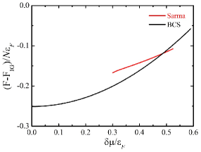
Figure 1: The free energy of both spin-population balanced BCS state (black line) and spin-polarized Sarma state (red line) at scattering length $1/k_{F}a_{0}=-0.5$, $1/k_{F}a_{1}=-0.05$ and Zeeman detuning $\delta(B)=0.4\varepsilon_{F}$. $F_{{\rm IG}}$ is the free energy of ideal Fermi gases with the same particle number.

With the language of Green’s function, we start with equations of motion of any operators $A$ and $B$ in the momentum-energy representation $\omega\left\langle\left\langle A|B\right\rangle\right\rangle_{\omega}=\left\langle\left[A,B\right]_{+}\right\rangle+\left\langle\left\langle\left[A,\mathcal{H}_{{\rm mf}}\right]|B\right\rangle\right\rangle_{\omega}$, and obtain three independent Green’s function

$$\begin{array}[]{cll}G_{1}^{\left(n\right)}\left(K\right)&\equiv\left\langle\left\langle c_{n1,k}|c_{n1,k}^{\dagger}\right\rangle\right\rangle_{\omega}&=\underset{l}{\sum}\frac{\frac{1}{2}\left(1+l\frac{\xi_{nk}}{E_{nk}}\right)}{i\omega-E_{nk}^{l}},\\ G_{2}^{\left(n\right)}\left(K\right)&\equiv\left\langle\left\langle c_{n2,k}|c_{n2,k}^{\dagger}\right\rangle\right\rangle_{\omega}&=\underset{l}{\sum}\frac{\frac{1}{2}\left(1-l\frac{\xi_{nk}}{E_{nk}}\right)}{i\omega+E_{nk}^{l}},\\ \Gamma^{\left(n\right)}\left(K\right)&\equiv\left\langle\left\langle c_{n1,k}|c_{n2,-k}\right\rangle\right\rangle_{\omega}&=\underset{l}{\sum}\frac{l\frac{\Delta_{n}}{2E_{nk}}}{i\omega-lE_{nk}^{l}},\end{array}$$ (11)

where $K=\left(k,i\omega\right)$ is a four-dimensional momentum, and $\begin{array}[]{cc}E_{nk}^{l}=-\delta\mu+lE_{nk},&E_{nk}=\sqrt{\xi_{nk}^{2}+\Delta_{n}^{2}}\end{array},$ $l=\pm 1$ stands for the particle or hole solution. These Green’s functions should be self-consistently solved with density equations

$$\rho_{o}=\sum_{k}\left\{1-\frac{\xi_{ok}}{E_{ok}}\left[1-f\left(E_{ok}^{+1}\right)-f\left(-E_{ok}^{-1}\right)\right]\right\},$$ (12)

$$\rho_{c}=\sum_{k}\left\{1-\frac{\xi_{ck}}{E_{ck}}\left[1-f\left(E_{ck}^{+1}\right)-f\left(-E_{ck}^{-1}\right)\right]\right\},$$ (13)

and order parameters equations

$$\frac{\lambda_{1}\Delta_{o}}{\Delta_{c}}+\lambda_{0}=\sum_{k}\left[\frac{M}{\hbar^{2}k^{2}}-\frac{1-f\left(E_{ck}^{+1}\right)-f\left(-E_{ck}^{-1}\right)}{2E_{ck}}\right]$$ (14)

$$\frac{\lambda_{1}\Delta_{c}}{\Delta_{o}}+\lambda_{0}=\sum_{k}\left[\frac{M}{\hbar^{2}k^{2}}-\frac{1-f\left(E_{ok}^{+1}\right)-f\left(-E_{ok}^{-1}\right)}{2E_{ok}}\right]$$ (15)

where

$$\begin{array}[]{cc}\lambda_{0}=+\frac{Ma_{0}}{4\pi\hbar^{2}\left(a_{0}^{2}-a_{1}^{2}\right)},&\lambda_{1}=-\frac{Ma_{1}}{4\pi\hbar^{2}\left(a_{0}^{2}-a_{1}^{2}\right)}\end{array},$$ (16)

and $f\left(x\right)=1/\left(e^{x/k_{B}T}+1\right)$ is the famous Fermi-Dirac distribution function. The free energy of the system in mean-field approximation reads

$$\begin{array}[]{cl}F_{{\rm mf}}=&-\Delta^{\dagger}\left[\begin{array}[]{cc}\lambda_{0}&\lambda_{1}\\ \lambda_{1}&\lambda_{0}\end{array}\right]\Delta+\underset{nk}{\sum}\left(\xi_{nk}-E_{nk}+\frac{\Delta_{n}^{2}M}{\hbar^{2}k^{2}}\right)\\ &-k_{B}T\underset{nkl}{\sum}{\rm ln}\left(1+e^{-E_{nk}^{l}/k_{B}T}\right)+\mu N\end{array}$$ (17)

where $\Delta\equiv\left[\begin{array}[]{cc}\Delta_{o},&\Delta_{c}\end{array}\right]^{T}$. As shown in Fig.1, a phase transition from a spin-balanced BCS superfluid to a spin-polarized Sarma superfluid is observed by continuously increasing chemical potential difference $\delta\mu$ over a critical value $\delta\mu_{{\rm cr}}=0.486\varepsilon_{F}$.

II.2 Random phase approximation and response function

The fluctuation term of interaction Hamiltonian plays a great role in the calculation of dynamics of the system, random phase approximation has been proved to be an effective way to collect the contribution from the fluctuation term. To introduce this story about how to obtain an accurate response function with random phase approximation approach, let us begin with the linear response theory.

In any superfluid state of OFR, there are usually four different densities in both open and close channels. Besides the normal spin-up and down densities ($\rho_{i}^{n}\equiv\left\langle\psi_{ni}^{\dagger}\psi_{ni}\right\rangle$, $i=1,2$), the other two are anomalous density $\rho_{3}^{n}\equiv\left\langle\psi_{n2}\psi_{n1}\right\rangle$ and its complex conjugate $\rho_{4}^{n}\equiv\left\langle\psi_{n1}^{\dagger}\psi_{n2}^{\dagger}\right\rangle$. When a weak external perturbation potential $V_{{\rm ext}}$ is imposed to all densities in two channels with form $V_{{\rm ext}}=\left[\begin{array}[]{cc}V^{o},&V^{c}\end{array}\right]^{T}$ and $V^{n}=\left[\begin{array}[]{cccc}V_{1}^{n},&V_{2}^{n},&V_{3}^{n},&V_{4}^{n}\end{array}\right]^{T}$, the corresponding perturbation Hamiltonian reads

$$H_{p}=\sum_{nkqj}\varPsi_{nk+q}^{\dagger}V_{j}^{n}\sigma_{j}\varPsi_{nk}$$ (18)

where $j=1,2,3,4$ stands for four different densities index in $n$ channel, and $\varPsi_{nk}=\left[\begin{array}[]{cc}c_{n1,k},&c_{n2,-k}^{\dagger}\end{array}\right]^{T}$ is the field operator in Nambu spinor representation. Also with Pauli matrices $\sigma_{x,y,z}$ and unit matrix $I$ we define $\sigma_{1}\equiv\left(I+\sigma_{z}\right)/2$, $\sigma_{2}\equiv\left(I-\sigma_{z}\right)/2$, $\sigma_{3}\equiv\left(\sigma_{x}-i\sigma_{y}\right)/2$ and $\sigma_{4}\equiv\left(\sigma_{x}+i\sigma_{y}\right)/2$. This perturbation Hamiltonian $H_{p}$ introduces a fluctuation of density matrix

$$\rho_{q}=\chi V_{{\rm ext}},$$ (19)

which connects to the external potential $V_{{\rm ext}}$ by the response function $\chi$ of the system.

$$\rho_{q}^{n}=\sum_{k}\left[\begin{array}[]{c}\varPsi_{nk}^{\dagger}\sigma_{1}\varPsi_{nk+q}\\ \varPsi_{nk}^{\dagger}\sigma_{2}\varPsi_{nk+q}\\ \varPsi_{nk}^{\dagger}\sigma_{3}\varPsi_{nk+q}\\ \varPsi_{nk}^{\dagger}\sigma_{4}\varPsi_{nk+q}\end{array}\right]$$ (20)

is the expression of density fluctuation in $n$ channel. Usually the exact calculation of response function $\chi$ is quite hard and difficult. However, random phase approximation suggests that we can treat the fluctuation term of interaction Hamiltonian $H_{{\rm sf}}=\sum_{nq}\rho_{q}^{n\dagger}\cdot A_{q}^{n}$ as a self-consistent dynamical potential $V_{{\rm sf}}^{n}=M_{I}A_{q}^{n},$ in which $A_{q}^{n}=\left[\begin{array}[]{cccc}0,&0,&\Delta_{n,q},&\Delta_{n,-q}^{*}\end{array}\right]^{T}$is the strength of fluctuation potential with

$$\left[\begin{array}[]{c}\Delta_{o,q}\\ \Delta_{o,-q}^{*}\\ \Delta_{c,q}\\ \Delta_{c,-q}^{*}\end{array}\right]=\sum_{k}\left[\begin{array}[]{cccc}V_{oo}&0&V_{oc}&0\\ 0&V_{oo}&0&V_{oc}\\ V_{co}&0&V_{cc}&0\\ 0&V_{co}&0&V_{cc}\end{array}\right]\left[\begin{array}[]{c}\left\langle\varPsi_{ok}^{\dagger}\sigma_{3}\varPsi_{ok+q}\right\rangle\\ \left\langle\varPsi_{ok}^{\dagger}\sigma_{4}\varPsi_{ok+q}\right\rangle\\ \left\langle\varPsi_{ck}^{\dagger}\sigma_{3}\varPsi_{ck+q}\right\rangle\\ \left\langle\varPsi_{ck}^{\dagger}\sigma_{4}\varPsi_{ck+q}\right\rangle\end{array}\right],$$ (21)

and $M_{I}$ is just a constant matrix

$$M_{I}=\left[\begin{array}[]{cccc}0&0&0&0\\ 0&0&0&0\\ 0&0&0&1\\ 0&0&1&0\end{array}\right].$$ (22)

We should notice that here we neglect the fluctuation from the normal spin-up and down density. This is reasonable in three dimensional space where the utilization of $s$-wave contact interaction induces two anomalous densities to be divergent, and play a much more important role than normal densities. Now the system can be treated as a mean-field quasiparticle gases experienced by an effective potential

$$V_{{\rm eff}}\equiv V_{{\rm ext}}+V_{{\rm sf}},$$ (23)

which induces the density fluctuations $\rho_{q}$ of the system following

$$\rho_{q}=\Pi\cdot V_{{\rm eff}},$$ (24)

in which $\Pi$ is the response function matrix in the mean-field level, whose calculation is feasible and relatively quite easy. Finally, with Eqs.19, 23 and 24, we find the desired response function $\chi$ can be calculated by its connection with mean-field response function $\Pi$ by

$$\chi=\frac{\Pi}{1-\Pi M_{G}},$$ (25)

where $M_{G}$ is another constant matrix

$$M_{G}=\left[\begin{array}[]{cc}M_{I}V_{oo},&M_{I}V_{oc}\\ M_{I}V_{co},&M_{I}V_{cc}\end{array}\right].$$ (26)

The mean-field response function $\Pi$ is a $8\times 8$ matrix, its explicit form is given by

$$\left[\begin{array}[]{cccccccc}\Pi_{11}^{o}&\Pi_{12}^{o}&\Pi_{13}^{o}&\Pi_{14}^{o}&0&0&0&0\\ \Pi_{12}^{o}&\Pi_{22}^{o}&\Pi_{23}^{o}&\Pi_{24}^{o}&0&0&0&0\\ \Pi_{14}^{o}&\Pi_{24}^{o}&-\Pi_{12}^{o}&\Pi_{34}^{o}&0&0&0&0\\ \Pi_{13}^{o}&\Pi_{23}^{o}&\Pi_{43}^{o}&-\Pi_{12}^{o}&0&0&0&0\\ 0&0&0&0&\Pi_{11}^{c}&\Pi_{12}^{c}&\Pi_{13}^{c}&\Pi_{14}^{c}\\ 0&0&0&0&\Pi_{12}^{c}&\Pi_{22}^{c}&\Pi_{23}^{c}&\Pi_{24}^{c}\\ 0&0&0&0&\Pi_{14}^{c}&\Pi_{24}^{c}&-\Pi_{12}^{c}&\Pi_{34}^{c}\\ 0&0&0&0&\Pi_{13}^{c}&\Pi_{23}^{c}&\Pi_{43}^{c}&-\Pi_{12}^{c}\end{array}\right].$$ (27)

Different from spin-population balanced case, there are $9$ independent matrix elements in mean-field response function of each channel, or $16$ matrix elements in two channels, which make the calculation of response function become much heavy. In the final appendix of this paper, we give all expressions of these independent matrix elements. Although there are no cross terms in matrix of Eq.27 between open and close channel, the coupling effect between these two channels is indeed existent. First, it is shown in the definition of two order parameters (Eq.9). Also the random phase approximation brings a correction to mean-field response function, which is shown in the denominator of Eq.25. This correction brings not only the coupling effect of these two channels, but also the right correction to investigate all collective excitations.

Finally, we obtain the intra and inter response functions between these two channels

$$\begin{array}[]{c}\chi^{\left(oo\right)}=\chi_{11}+\chi_{12}+\chi_{21}+\chi_{22},\\ \chi^{\left(oc\right)}=\chi_{15}+\chi_{16}+\chi_{25}+\chi_{26},\\ \chi^{\left(co\right)}=\chi_{51}+\chi_{52}+\chi_{61}+\chi_{62},\\ \chi^{\left(cc\right)}=\chi_{55}+\chi_{56}+\chi_{65}+\chi_{66}.\end{array}$$ (28)

II.3 Dynamic structure factors

We now turn to discuss dynamic structure factors (DSF for short). Similarly we can define the intra and inter dynamic structure factor between two channels, which here is named the total and relative density dynamic structure factor, respectively zhang2016 ,

$$S_{{\rm tot}}\left(q,\omega\right)=-\frac{{\rm Im\left[\chi^{\left(oo\right)}+\chi^{\left(oc\right)}+\chi^{\left(co\right)}+\chi^{\left(cc\right)}\right]}}{\pi\left(1-e^{-\hbar\omega/k_{B}T}\right)},$$ (29)

$$S_{{\rm rel}}\left(q,\omega\right)=-\frac{{\rm Im\left[\chi^{\left(oo\right)}-\chi^{\left(oc\right)}-\chi^{\left(co\right)}+\chi^{\left(cc\right)}\right]}}{\pi\left(1-e^{-\hbar\omega/k_{B}T}\right)},$$ (30)

where the subscript ’rel’ denotes a relative density oscillation between the open and close channel. The total density dynamic structure factor satisfies the famous $f$-sum rule

$$\int d\omega S_{{\rm tot}}\left(q,\omega\right)\omega=N\frac{q^{2}}{2M},$$ (31)

while at limit $q\rightarrow 0$ the relative density dynamic structure factor satisfies

$$\int d\omega S_{{\rm rel}}\left(q,\omega\right)\omega=N\frac{q^{2}}{2M}-8\left\langle V_{oc}\right\rangle,$$ (32)

where $\langle V_{oc}\rangle$ is the coupling energy between open and closed channels zhang2016 . In our following discussion, we will focus on zero temperature $T=0$, and set Plank constant $\hbar=1$ for simple.

III DSF in balanced BCS superfluid

Let us first overview a spin-population balanced case with chemical potential difference $\delta\mu=0$. The ground state of the system is a BCS-type superfluid in both open and close channel, namely $\left[{\rm BCS}\right]_{o}\left[{\rm BCS}\right]_{c}$. There are two stable eigenstates, one is in-phase state with order parameters satisfy $\Delta_{o}\Delta_{c}>0$, and the other one is an out-of-phase state with $\Delta_{o}\Delta_{c}<0$. Both of them are possible candidates of ground state, depending on specific interaction parameters. The collective excitation at transferred momentum $q\ll k_{F}$ or $q\sim k_{F}$ had been discussed in Ref. zhang2016 . We will first focus our discussion on a large transferred momentum $q\gg k_{F}$, and then discuss the situation related to phase transition.

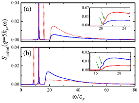
Figure 2: The total density dynamic structure factor (blue line) and relative one(red line) of BCS superfluid in in-phase ground state (a) and out-of-phase metastable state (b). Two inset figures are their own enlarge of the pair-breaking excitation, the left and right arrow mark the initial position of pair-breaking excitation in the open and closed channel, respectively.

We take interaction parameters $1/k_{F}a_{0}=12/7$ and $1/k_{F}a_{1}=-12$ (or $1/k_{F}a_{-}=2.0$ and $1/k_{F}a_{+}=1.5$), at which the system is in the BEC regime of the famous BCS-BEC crossover. Then in-phase state is the ground state, while the out-of-state is an energetical metastable state. We set Zeeman detuning $\delta\left(B\right)=0.5\varepsilon_{F}$. The results of total and relative dynamic structure factors of in-phase and out-of-phase state at transferred momentum $q=5k_{F}$ are shown in Fig.2. Panel (a) is from the in-phase state with chemical potential $\mu=-3.83\varepsilon_{F}$, open channel order parameter $\Delta_{o}=1.38\varepsilon_{F}$ and close channel one $\Delta_{c}=1.23\varepsilon_{F}$, while panel (b) from out-of-phase state with $\mu=-2.05\varepsilon_{F}$, $\Delta_{o}=1.03\varepsilon_{F}$ and $\Delta_{c}=-1.23\varepsilon_{F}$. Something in common in these two panels is that, all dynamic structure factors consist of four different excitations, which are molecular excitation, collective Leggett mode and Cooper-pair breaking excitation in both open and close channel. The molecular excitation of both panels always locates at $q^{2}/4M\simeq 12.5\varepsilon_{F}$, which are only dependent on the value of transferred momentum $q$, no matter what state it is. Since the chemical potential in two states both satisfy $\mu<0$, the minimum energy required to break a Cooper-pair is $\omega_{th}^{\left(o\right)}=2\sqrt{(q^{2}/8M-\mu)^{2}+\Delta_{o}^{2}}$ in open channel and $\omega_{th}^{\left(c\right)}=2\sqrt{(q^{2}/8M-\mu+\delta\left(B\right)/2)^{2}+\Delta_{c}^{2}}$ in close channel, respectively. These two initial excitations generate two twist points in two inset figures, located by two arrows. Panel (a) is the ground state because the in-phase state requires more energy to break a Cooper-pair than the case of out-of-phase state shown in Panel (b). This is also proved by a relatively longer energy distance between molecular excitation and ${\rm min}\left[\omega_{th}^{\left(o\right)},\omega_{th}^{\left(c\right)}\right]$, whose value is almost equal to the bigger bound energy $\varepsilon_{b}^{-}=-\hbar^{2}/Ma_{-}^{2}=8.0\varepsilon_{F}$, while the energy distance between Leggett mode and ${\rm min}\left[\omega_{th}^{\left(o\right)},\omega_{th}^{\left(c\right)}\right]$ take the other smaller bound energy $\varepsilon_{b}^{+}=-\hbar^{2}/Ma_{+}^{2}$ (these two energy differences will be exactly equal to $\varepsilon_{b}^{\pm}=-\hbar^{2}/Ma_{\pm}^{2}=4.5\varepsilon_{F}$ when $\delta\left(B\right)=0$). This is also the reason why the Leggett mode locates on the right hand side of molecular excitation in Panel (a), or on the left hand side in Panel (b). Here dynamic structure factors display rich information about large transferred momentum dynamical excitations, which do a great help to distinguish ground in-phase state from metastable out-of-phase state.

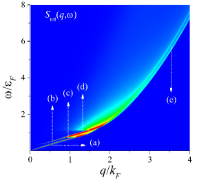
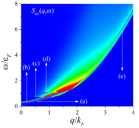
Figure 3: The total (upper panel) and relative (lower panel) dynamic structure factor in BCS superfluid side of phase transition, with scattering length $1/k_{F}a_{0}=-0.5$, $1/k_{F}a_{1}=-0.05$, Zeeman detuning $\delta(B)=0.4\varepsilon_{F}$. The result is independent on the value of chemical potential difference when $\delta\mu<\delta\mu_{{\rm cr}}$. (a) phonon mode, (b) Leggett mode, (c) $2\Delta_{c}$, (d) $2\Delta_{o}$, (e) pair-breaking excitations at a large $q$ in two channels.

Next we discuss the phase transition from BCS to Sarma superfluid with the same parameters in Fig.1. When chemical potential difference $\delta\mu$ is smaller than the critical value $\delta\mu_{{\rm cr}}=0.486\varepsilon_{F}$, a BCS superfluid state becomes the ground state of the system. These parameters are like the results of single-channel Fermi superfluid close to unitary regime of BCS-BEC crossover, with a positive chemical $\mu=0.43\varepsilon_{F}$. As shown in Fig.3, at a small transferred momentum $q$, we observe two collective excitations (red curves in two panels), the phonon (a) and Leggett mode (b). Relatively, the gapless phonon mode is easier to investigate in total dynamic structure factor than in the relative dynamic structure factor, while the gapped Leggett mode just in inverse. Two short horizontal lines at $\omega^{\left(c\right)}=2|\Delta_{c}|=0.72\varepsilon_{F}$ (c) and $\omega^{\left(o\right)}=2|\Delta_{o}|=1.10\varepsilon_{F}$ (d) represent two minimum values of energy to break a Cooper pair in open and close channel, respectively, while the same physics evolves into a two-peak signal at a large $q$ (e). Here in fact all results are independent the value of chemical potential difference $\delta\mu$, when $\delta\mu<\delta\mu_{{\rm cr}}$. The system is always a spin-population balanced BCS superfluid state.

IV DSF in Sarma superfluid

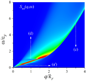
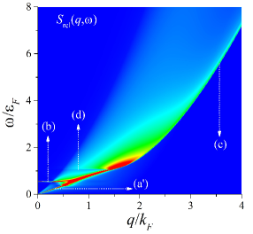
Figure 4: The total (upper panel) and relative (lower panel) dynamic structure factor in Sarma superfluid side of phase transition, with scattering length $1/k_{F}a_{0}=-0.5$, $1/k_{F}a_{1}=-0.05$, Zeeman detuning $\delta(B)=0.4\varepsilon_{F}$, and chemical potential difference $\delta\mu=0.5\varepsilon_{F}$. (${\rm a^{\prime}}$) phonon mode mixed with single-particle gapless excitation in close channel, (b) Leggett mode, (d) $2\Delta_{o}$, (e) pair-breaking excitations at a large $q$ in two channels.

For the same scattering length $1/k_{F}a_{0}=-0.5$, $1/k_{F}a_{1}=-0.05$ and Zeeman detuning $\delta(B)=0.4\varepsilon_{F}$, but varying the chemical potential difference over the critical value $\delta\mu_{{\rm cr}}$ to $\delta\mu=0.5\varepsilon_{F}$, the system comes into a spin-population polarized Sarma superfluid state $\left[{\rm BCS}\right]_{o}\left[{\rm Sarma}\right]_{c}$. The chemical potential difference $\delta\mu$ is larger than the order parameter in close channel $\Delta_{c}=-0.08\varepsilon_{F}$, but smaller than one in open channel $\Delta_{o}=0.54\varepsilon_{F}$. Then the close channel becomes a gapless Sarma superfluid, while the open channel is a BCS superfluid. Our main results of the total and relative dynamic structure factor in this Sarma superfluid are shown respectively in two panels of Fig.4, in the form of two-dimensional contour plot in the $q$-$\omega$ plane. The dynamic structure factors as a function of $\omega$ at small and large transferred momenta are reported in Fig.5 and Fig.6, respectively.

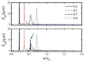
Figure 5: The total (upper panel) and relative (lower panel) dynamic structure factors of Sarma superfluid at small transferred momentums, $q=0.3,0.5,0.7,0.9k_{F}$. A green arrow in lower panel locates the Leggett mode.

Different from the results of BCS superfluid whose phonon excitation has an obvious delta-like structure, the phonon excitation here has a finite expansion width because of the scattering with the gapless single-particle excitation in the close channel, which is denoted as (${\rm a^{\prime}}$) in Fig.4. In greater detail, all collective excitations are focused in a small transferred momentum $q$ regime $\left(q<k_{F}\right)$. A single-particle gapless excitation of Sarma superfluid can be observed in both total and relative dynamic structure factors, and it is mixed with another gapless excitation, the collective phonon excitation. This monotonically increasing linear behavior of dynamic structure factor is also displayed in Fig.6 at $q=2k_{F}$, where the transferred energy starts from a very small value. The results in this regime are quite similar to behavior of ideal Fermi gases mazzanti1996 , and it can be understood from the fact that some fermionic atoms are not paired, and behave like free fermions in close channel. This gapless dynamical behavior is the most specific character of Sarma superfluid.

Also we can observe an horizontal gapped Leggett excitation, whose position almost does not vary with the transferred momentum $q$. This is also shown in the peak around $\omega\simeq 0.6\varepsilon_{F}$ of relative dynamic structure factor in Fig.5, located by a green arrow. Going on increasing transferred momentum $q$, a merge procedure between Leggett and phonon mode can be clearly investigated in the relative dynamic structure factor (Panel (b) of Fig.4, and lower panel of Fig.5), the critical value of transferred momentum is around $q\approx 0.7k_{F}$, after which the phonon and Leggett excitations are mixed together and show only a wide peak, as shown by gray dot line in Fig.5.

Another physics we are interested in is the minimum value to break Cooper pairs in two channels. Different from the BCS superfluid, only one short horizontal line at $\omega^{(o)}=2\Delta_{o}=1.08\varepsilon_{F}$, who is the minimum energy to break a Cooper-pair in open channel, is observed, while the other one in close channel is completely immersed in the gapless excitation.

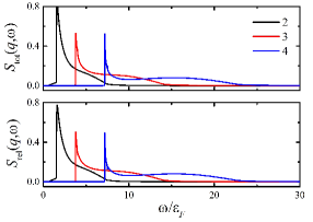
Figure 6: The total (upper panel) and relative (lower panel) dynamic structure factors of Sarma superfluid at big transferred momentums, $q=2,3,4k_{F}$.

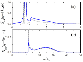
Figure 7: The comparison of total dynamic structure factor between BCS superfluid state (blue line) and Sarma superfluid state (grey dot line) at $q=1k_{F}$ (a) and $q=5k_{F}$ (b).

At a large $q$, the molecular excitation and atomic excitation are both observed in Fig.6 and Panel (b) of Fig.7. Different from the BCS superfluid, the molecular excitation does not have a clear two-peak signal related to pair-breaking excitations in two channels, which is because that the Cooper pair breaking in close channel is quite weak, compared with one in open channel. We can only observe a very small peak in total dynamic structure factors, or a very small dip in relative dynamic structure factors, whose location is after the first big Cooper-pair breaking peak in Fig.6. The atomic excitation, whose location is around $q^{2}/2M$, becomes more and more obvious when increasing transferred momentum $q$. Also Sarma superfluid has a relative stronger atomic excitation than one in BCS superfluid since it has more surplus of unpaired Fermi atoms.

Finally we give Fig.7 by which to present the main difference between BCS superfluid (gray line) and Sarma superfluid (blue line). Compared with BCS superfluid, Sarma superfluid has a linear gapless excitation at $q=k_{F}$, mixed with the collective phonon excitation (Panel (a)), and a stronger atomic excitation (Panel (b)) at $q=5k_{F}$.

V Conclusions

In summary, we investigate dynamic structure factors of a two-channel Fermi superfluid with orbital Feshbach resonance. In spin-population balanced BCS superfluid state, dynamic structure factors can do help to distinguish the ground in-phase from metastable out-of-phase state by the location of minimum energy to break a Cooper-pair, or the relative location between collective Leggett mode and molecular excitation in a BEC-like parameters regime. For another different interaction parameters where Sarma superfluid may replace the BCS superfluid as a possible ground state of the system, we numerically calculate dynamic structure factors and find their dynamical characters in both spin-population balanced BCS superfluid and spin-polarized Sarma superfluid. An obvious gapless excitation at a small transferred energy is observed only in Sarma superfluid, which also has a stronger atomic excitation at a large transferred momentum. These discoveries can serve to differentiate all possible eigenstates of the system.

VI Acknowledgement

Our research was supported by the National Natural Science Foundation of China, Grants No. 11804177 (P.Z.), No. 11547034 (H.Z.) and No. 11775123 (L.H.), by the Shandong Provincial Natural Science Foundation, China, Grant No. ZR2018BA032 (P.Z.), and by Australian Research Council’s (ARC) Discovery Projects No. DP180102018 (X.-J.L), and No. DP170104008 (H.H.). L.H. acknowledges the support of the Recruitment Program for Young Professionals in China (i.e., the Thousand Young Talent Program).

VI.1 Appendix

In this appendix, we will give the derivation of mean-field response functions $\Pi$ in both open and close channels. Actually the response functions in these two channels are the same as each other, but with their corresponding values of chemical potential $\mu_{n}$ and order parameter $\Delta_{n}$ , where $n=o,c$ is the channel index. For example, in $n$ channel, there are $9$ independent matrix elements, which are expressed as

$$\Pi_{11}^{n}\left(q,\omega\right)=+\sum_{kll^{\prime}}P_{1}^{l}\left(k\right)P_{1}^{l^{\prime}}\left(k+q\right)F_{k}^{ll^{\prime}}\left(q,\omega\right),$$

$$\Pi_{12}^{n}\left(q,\omega\right)=-\sum_{kll^{\prime}}P_{3}^{l}\left(k\right)P_{3}^{l^{\prime}}\left(k+q\right)F_{k}^{ll^{\prime}}\left(q,\omega\right),$$

$$\Pi_{13}^{n}\left(q,\omega\right)=-\sum_{kll^{\prime}}P_{1}^{l}\left(k\right)P_{3}^{l^{\prime}}\left(k+q\right)F_{k}^{ll^{\prime}}\left(q,\omega\right),$$

$$\Pi_{14}^{n}\left(q,\omega\right)=-\sum_{kll^{\prime}}P_{3}^{l}\left(k\right)P_{1}^{l^{\prime}}\left(k+q\right)F_{k}^{ll^{\prime}}\left(q,\omega\right),$$

$$\Pi_{22}^{n}\left(q,\omega\right)=+\sum_{kll^{\prime}}P_{2}^{l}\left(k\right)P_{2}^{l^{\prime}}\left(k+q\right)F_{k}^{ll^{\prime}}\left(q,\omega\right),$$

$$\Pi_{23}^{n}\left(q,\omega\right)=+\sum_{kll^{\prime}}P_{3}^{l}\left(k\right)P_{2}^{l^{\prime}}\left(k+q\right)F_{k}^{ll^{\prime}}\left(q,\omega\right),$$

$$\Pi_{24}^{n}\left(q,\omega\right)=+\sum_{kll^{\prime}}P_{2}^{l}\left(k\right)P_{3}^{l^{\prime}}\left(k+q\right)F_{k}^{ll^{\prime}}\left(q,\omega\right),$$

$$\Pi_{34}^{n}\left(q,\omega\right)=+\sum_{kll^{\prime}}P_{2}^{l}\left(k\right)P_{1}^{l^{\prime}}\left(k+q\right)F_{k}^{ll^{\prime}}\left(q,\omega\right),$$

$$\Pi_{43}^{n}\left(q,\omega\right)=+\sum_{kll^{\prime}}P_{1}^{l}\left(k\right)P_{2}^{l^{\prime}}\left(k+q\right)F_{k}^{ll^{\prime}}\left(q,\omega\right),$$

where

$$P_{1}^{l}\left(k\right)=\frac{1}{2}\left(1+l\frac{\xi_{nk}}{E_{nk}}\right),$$

$$P_{2}^{l}\left(k\right)=\frac{1}{2}\left(1-l\frac{\xi_{nk}}{E_{nk}}\right),$$

$$P_{3}^{l}\left(k\right)=l\frac{\Delta_{n}}{2E_{nk}},$$

$$F_{k}^{ll^{\prime}}\left(q,\omega\right)=\frac{f\left(E_{nk}^{l}\right)-f\left(E_{nk+q}^{l^{\prime}}\right)}{\omega+i\eta+E_{nk}^{l}-E_{nk+q}^{l^{\prime}}}.$$

$q$ and $\omega$ are respectively the transferred momentum and energy, $l=\pm 1$ stands for the particle or hole solution, $\eta$ is a small positive number. Specifically one should notice that expressions of $\Pi_{34}^{n}$ and $\Pi_{43}^{n}$ are both divergent. The random phase approximation, shown in the denominator of Eq.25, do help to cure the divergence of them.

References

- (1) L. Pitaevskii and S. Stringari, Bose-Einstein Condensation, (Oxford: Oxford University Press, 2003).
- (2) M. G. Lingham, K. Fenech, S. Hoinka, and C. J. Vale, Local Observation of Pair Condensation in a Fermi Gas at Unitarity, Phys. Rev. Lett. 112, 100404 (2014).
- (3) E. D. Kuhnle, S. Hoinka, P. Dyke, H. Hu, P. Hannaford, and C. J. Vale, Temperature Dependence of the Universal Contact Parameter in a Unitary Fermi Gas, Phys. Rev. Lett. 106, 170402 (2011).
- (4) S. Hoinka, M. Lingham, K. Fenech, H. Hu, C. J. Vale, J. E. Drut, and S. Gandolfi, Precise Determination of the Structure Factor and Contact in a Unitary Fermi Gas, Phys. Rev. Lett. 110, 055305 (2013).
- (5) G. Veeravalli, E. Kuhnle, P. Dyke, and C. J. Vale, Bragg Spectroscopy of a Strongly Interacting Fermi Gas, Phys. Rev. Lett. 101, 250403 (2008).
- (6) S. Hoinka, M. Lingham, M. Delehaye, and C. J. Vale, Dynamic Spin Response of a Strongly Interacting Fermi Gas, Phys. Rev. Lett. 109, 050403 (2012).
- (7) Sascha Hoinka, Paul Dyke, Marcus G. Lingham, Jami J. Kinnunen, Georg M. Bruun and Chris J. Vale, Goldstone mode and pair-breaking excitations in atomic Fermi superfluids, Nat. Phys. 13, 943 (2017).
- (8) A. Brunello, F. Dalfovo, L. Pitaevskii, S. Stringari, and F. Zambelli, Momentum transferred to a trapped Bose-Einstein condensate by stimulated light scattering, Phys. Rev. A 64, 063614 (2001).
- (9) P. Fulde and R. A. Ferrell, Superconductivity in a Strong Spin-Exchange Field, Phys. Rev. 135, A550 (1964).
- (10) A. I. Larkin and Y. N. Ovchinnikov, Nonuniform state of superconductors, Zh. Eksp. Teor. Fiz. 47, 1136 (1964) [Sov. Phys. JETP 20, 762 (1965)].
- (11) G. Sarma, On the influence of a uniform exchange field acting on the spins of the conduction electrons in a superconductor, J. Phys. Chem. Solids 24, 1029 (1963).
- (12) C. Zhang, S. Tewari, R. M. Lutchyn, and S. D. Sarma, Superfluid from -Wave Interactions of Fermionic Cold Atoms, Phys. Rev. Lett. 101, 160401 (2008).
- (13) L. He and P. Zhuang, Stable Sarma state in two-band Fermi systems, Phys. Rev. B 79, 024511 (2009).
- (14) R. Zhang, Y. Cheng, H. Zhai, and P. Zhang, Orbital Feshbach resonance in Alkali-Earth Atoms, Phys. Rev. Lett. 115, 135301 (2015).
- (15) P. Zou, L. He, X. -J. Liu,and Hui Hu, Strongly interacting Sarma superfluid near orbital Feshbach resonances, Phys. Rev. A 97, 043618 (2018).
- (16) G. Pagano, M. Mancini, G. Cappellini, L. Livi, C. Sias, J. Catani, M. Inguscio, and L. Fallani, Strongly Interacting Gas of Two-Electron Fermions at an Orbital Feshbach Resonance, Phys. Rev. Lett. 115, 265301 (2015).
- (17) M. Höfer, L. Riegger, F. Scazza, C. Hofrichter, D. R. Fernandes, M. M. Parish, J. Levinsen, I. Bloch, and S. Fölling, Observation of an Orbital Interaction-Induced Feshbach Resonance in 173Yb, Phys. Rev. Lett. 115, 265302 (2015).
- (18) A. J. Leggett, Number-phase fluctuations in two-band superconductors, Prog. Theor. Phys. 36, 901 (1966).
- (19) G. Blumberg, A. Mialitsin, B. S. Dennis, M. V. Klein, N. D. Zhigadlo, and J. Karpinski, Observation of Leggett’s Collective Mode in a Multiband Superconductor, Phys. Rev. Lett. 99, 227002 (2007).
- (20) S.-Z. Lin and X. Hu, Massless Leggett Mode in Three-Band Superconductors with Time-Reversal-Symmetry Breaking, Phys. Rev. Lett. 108, 177005 (2012).
- (21) N. Bittner, D. Einzel, L. Klam, and D. Manske, Leggett Modes and the Anderson-Higgs Mechanism in Superconductors without Inversion Symmetry. Phys. Rev. Lett. 115, 227002 (2015).
- (22) S. N. Klimin, H. Kurkjian and J. Tempere, Leggett collective excitations in a two-band Fermi superfluid at finite temperatures, New J. Phys. 21, 113043 (2019).
- (23) J. Xu, R. Zhang, Y. Cheng. P. Zhang, R. Qi, and H. Zhai, Reaching a Fermi-superfluid state near an orbital Feshbach resonance, Phys. Rev. A 94, 033609 (2016).
- (24) L. He, H. Hu, and X.-J. Liu, Two-band description of resonant superfluidity in atomic Fermi gases, Phys. Rev. A 91, 023622 (2015).
- (25) L. He, J. Wang, S.-G. Peng, X.-J. Liu, and H. Hu, Strongly correlated Fermi superfluid near an orbital Feshbach resonance: Stability, equation of state, and Leggett mode, Phys. Rev. A. 94, 043624 (2016).
- (26) H. Guo, C.-C. Chien, and Y. He, Theories of Linear Response in BCS Superfluids and How They Meet Fundamental Constraints, J. Low Temp. Phys. 172, 5 (2013).
- (27) L. He, Dynamic density and spin responses of a superfluid Fermi gas in the BCS-BEC crossover: Path integral formulation and pair fluctuation theory, Ann. Phys. 373, 470 (2016).
- (28) Y.-C. Zhang, S. Ding, and S. Zhang, Collective modes in a two-band superfluid of ultracold alkaline-earth-metal atoms close to an orbital Feshbach resonance, Phys. Rev. A 95, 041603(R) (2017).
- (29) F. Mazzanti, A. Polls, J. Boronat, Coherent and incoherent dynamic structure functions of the free Fermi gas, Phys. Lett. A, 220 (1996), p. 251.