Document Graph for Neural Machine Translation
Abstract
Previous works have shown that contextual information can improve the performance of neural machine translation (NMT). However, most existing document-level NMT methods only consider a few number of previous sentences. How to make use of the whole document as global contexts is still a challenge. To address this issue, we hypothesize that a document can be represented as a graph that connects relevant contexts regardless of their distances. We employ several types of relations, including adjacency, syntactic dependency, lexical consistency, and coreference, to construct the document graph. Then, we incorporate both source and target graphs into the conventional Transformer architecture with graph convolutional networks. Experiments on various NMT benchmarks, including IWSLT English–French, Chinese-English, WMT English–German and Opensubtitle English–Russian, demonstrate that using document graphs can significantly improve the translation quality. Extensive analysis verifies that the document graph is beneficial for capturing discourse phenomena.
1 Introduction
Although neural machine translation (NMT) has achieved great success on sentence-level translation tasks, many studies pointed out that translation mistakes become more noticeable at the document-level Wang et al. (2017); Tiedemann and Scherrer (2017); Zhang et al. (2018); Miculicich et al. (2018); Kuang et al. (2018); Voita et al. (2018); Läubli et al. (2018); Tu et al. (2018); Voita et al. (2019b); Kim et al. (2019); Yang et al. (2019). They proved that these mistakes can be alleviated by feeding the contexts into context-agnostic NMT models.
Previous works have explored various methods to integrate context information into NMT models. They usually take a limited number of previous sentences as contexts and learn context-aware representations using hierarchical networks (Miculicich et al., 2018; Wang et al., 2017; Tan et al., 2019) or extra context encoders (Jean et al., 2015; Zhang et al., 2018; Yang et al., 2019). Different from representation-based approaches, Tu et al. Tu et al. (2018) and Kuang et al. Kuang et al. (2018) propose using a cache to memorize context information, which can be either history hidden states or lexicons. To keep tracking of most recent contexts, the cache is updated when new translations are generated. Therefore, long-distance contexts would likely be erased.
How to use long-distance contexts is drawing attention in recent years. Approaches, like treating the whole document as a long sentence Junczys-Dowmunt (2019) and using memory and hierarchical structures Maruf and Haffari (2018); Maruf et al. (2019); Tan et al. (2019), are proposed to take global contexts into consideration. However, Kim et al. Kim et al. (2019) point out that not all the words in a document are beneficial to context integration, suggesting that it is essential for each word to focus on its own relevant context.

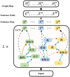
To address this problem, we suppose to build a document graph for a document, where each word is connected to those words which have a direct influence on its translation. Figure 2 shows an example of a document graph. Explicitly, a document graph is defined as a directed graph where: (1) each node represents a word in the document; (2) each edge represents one of the following relations between words: (a) adjacency; (b) syntactic dependency; (c) lexical consistency; or (d) coreference.
We apply a Graph Convolutional Network (GCN) on the document graph to obtain a document-level contextual representation for each word, fed to the conventional Transformer model (Vaswani et al., 2017) by additional attention and gating mechanisms. We evaluate our model on four translation benchmarks, IWSLT English–French (En–Fr) and Chinese–English (Zh–En), Opensubtitle English–Russian (En–Ru), and WMT English–German (En–De). Experimental results demonstrate that our approach is consistently superior to previous works Miculicich et al. (2018); Tu et al. (2018); Zhang et al. (2018); Macé and Servan (2019); Tan et al. (2019); Maruf et al. (2019) on all the language pairs.
Contributions of this work are summarized as:
-
•
We represent a document as a graph that connects relevant contexts regardless of their distances. To the best of our knowledge, this is the first work to introduce such graphs into document-level neural machine translation.
-
•
We investigate several relations between words to construct document graphs and verify their effectiveness in experiments.
-
•
We propose a graph encoder to learn graph representations based on GCN layers with an attention mechanism to combine representations of different sources.
-
•
We proposed a context integration method that examined the proposed graph model in different context-aware MT architectures.
2 Approach
In this section, we introduce the proposed document graph and model for leveraging contextual information from documents. Firstly, we present a definition of the problem. Then, the construction and representation learning of document graphs are explained in Section 2.2 and Section 2.3, respectively. Finally, we describe the method of integrating document graphs and model architectures that we use to examine the integration.
2.1 Problem Definition
Document-level NMT learns to translate from a document in a source language to a document in a target language. Formally, a source document is a set of sentences , where indicates the th sentence of the document. The corresponding target document is , where is a translation of the source sentence .
Given the source document to translate, we assume that there is a pair of source and target hidden graphs (called document graphs and defined in Section 2.2) to help generate the target document. Therefore, the translation probability from to can be represented as:
| (1) | |||
| (2) |
Equation (1) is computationally intractable. Therefore, instead of considering all possible graph pairs, we only sample one pair of graphs according to the source document resulting in a simplified Equation (2). The construction of source and target graphs are described in Section 2.2.
The translation of a document is further decomposed into translations of each sentence with document graphs as context:
| (3) |
2.2 Graph Construction
Graphs used in this paper are directed, which can be represented as , where is a set of nodes and is a set of edges where an edge with denotes an arrow connection from the node to the node .
Our graph contains both word-level and sentence-level nodes. Given a document where is the th () word in the th () sentence, we construct a document graph with word-level nodes and sentence-level nodes. Each word-level node in the th sentence is directly connected to the sentence-level node . Edges between word-level nodes are determined by intra-sentential and inter-sentential relations. Figure 2 shows an example document graph. Note that not all edges are depicted for simplicity.
Intra-sentential Relations
provide links between words in a sentence . These links are relatively local yet informative and help understand the structure and meaning of the sentence. In this paper, we consider two kinds of intra-sentential relations:
-
•
Adjacency provides a local lexicalized context that can be obtained without resorting to external resources and has been proven beneficial to sentence modeling Yang et al. (2018); Xu et al. (2019). For each word , we add two edges and . This means we add links from the current word to its adjacent words.
-
•
Dependency directly models syntactic and semantic relations between two words in a sentence. Dependency relations not only provide linguistic meanings but also allow connections between words with a longer distance. Previous practices have shown that dependency relations enhance representation learning of words Marcheggiani and Titov (2017); Strubell et al. (2018); Lin et al. (2019). Given a dependency tree of the sentence and a word , we add a graph edge if is a headword of .
Inter-sentential Relations
allow links from one sentence to another following sentence . These relations provide discourse information, which is important for capturing document phenomena in document-level NMT Tiedemann and Scherrer (2017); Voita et al. (2018). Accordingly, we consider two kinds of relations in our document graph:
-
•
Lexical consistency considers repeated and similar words across sentences in the document, which reflects the cohesion of lexical choices. In this paper, we add edges if or . Namely, the exact same words and words with the same lemma in the two sentences are connected in the graph.
-
•
Coreference is a common phenomenon in documents and exists when referring back to someone or something previously mentioned. It helps understand the logic and structure of the document and resolve the ambiguities. In this paper we add a graph edge if is a referent of given by coreference resolution.
Inter-sentential relations also exist between words in the same sentence, where .
Source and Target Graphs
In this paper, we construct a source graph directly from a source document using the method mentioned above. The target graph is built incrementally during inference, i.e., translations of previous sentences in the same document are used as target context. For simplicity, each target context sentence is treated as a fully connected graph and encoded independently by the graph encoder.
2.3 Document Graph Encoder
As the document is projected into a document graph, a flexible graph encoder is required to encode the complex structure. Previous studies verified that GCNs can be applied to encode linguistic structures such as dependency trees Marcheggiani and Titov (2017); Bastings et al. (2017); Koncel-Kedziorski et al. (2019); Huang et al. (2020). In this paper, we follow previous practices to use stacked GCN layers as the encoder of document graph with considerations on edge directions.
Graph Convolutional Networks
GCNs are neural networks operating on graphs and aggregating information from immediate neighbors of nodes. Information of longer-distance nodes is covered by stacking GCN layers. Formally, given a graph , the GCN network first projects the nodes into representations , where stands for hidden size and . Node representations of the th layer can be updated as follows:
| (4) |
where is the sigmoid function and are learnable parameters, is an adjacency matrix that stores edge information:
| (5) |
The degree matrix is assigned to weight the expected importance of a current node based on the number of input nodes, which can be calculated with the adjacency matrix:
| (6) |
Fusion of Edge Information
Equation (5) only considers input features. To fully use direction information in the graph, we apply GCN on different types of edges:
| (7) |
where represents one of the edge types, i.e., input edges, output edges, or a specific type of self-loop edges. We assume the contributions of the representations learned from a different kind of edges should be different. We then apply a type-attention mechanism, which works better than a linear combination in our experiments,333We report our experiments in Section 2 of Supplementary. to combine these representations of different edge types:
| (8) | ||||
| (9) |
where the are attention weights given by a dot-product attention algorithm Vaswani et al. (2017).
Sentence Embedding
After the GCN, we extract the sentence-level nodes as context representation. Since the GCN ignores explicitly positional information between sentences, we add a sentence embedding before integrating the context representation into an encoder or decoder. Figure 2 shows our graph encoder.
2.4 Integration of Context Representation
Context representation from the document graph encoder is treated as a memory and used by an attention mechanism, namely:
| (10) |
where Context-Attn is a multi-head attention function Vaswani et al. (2017). Instead of using the standard residual connection in this sublayer, we adopt a gated mechanism following Zhang et al. Zhang et al. (2019) to dynamically control the influence of context information:
| (11) | ||||
| (12) |
where are gating weights, and denotes the sigmoid function. and are the trainable parameters. In the rest of this paper, we use Context-Attn to denote both the attention and gated residual mechanisms.
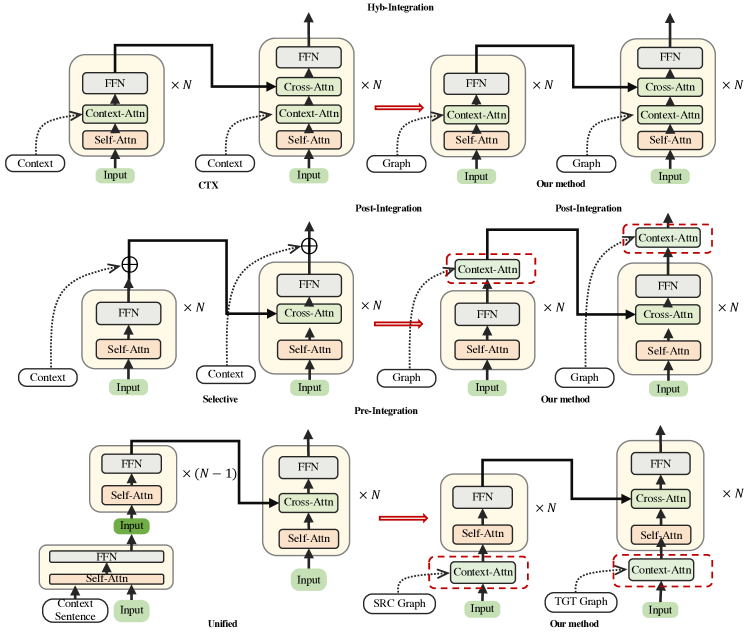
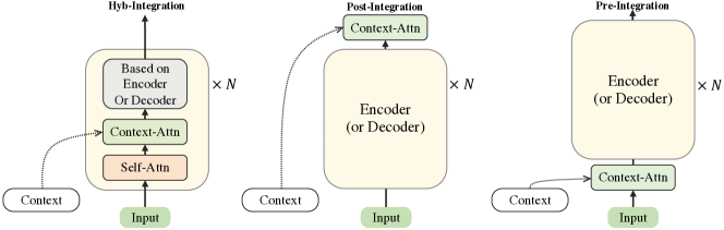
In this paper, the Context-Attn sublayer is used in three different ways, as shown in Figure 3:
3 Experiments
Data
We evaluate our approach on translation benchmarks with different corpus size: (1) IWSLT En–Fr and Zh–En translation tasks Cettolo et al. (2012) with around 200K sentence pairs for training. Following convention Wang et al. (2017); Miculicich et al. (2018); Zhang et al. (2018), both language pairs take dev2010 as the development set. tst2010 is used for testing on En–Fr and tst2010tst2013 on Zh–En. (2) Opensubtitle2018 En–Ru translation corpus released by Voita et al. Voita et al. (2018), which contains 6M sentence pairs for training, among which 1.5M sentence pairs have context sentences. (3) We adopted the WMT19 document-level corpus published by Scherrer et al. (2019) for the En-De translation task. This data contains 2.9M parallel sentences with document boundaries and 10.3M back-translated sentence pairs.
All data are tokenized and segmented into subword units using the byte-pair encoding Sennrich et al. (2016). We apply 32k merge steps for each language on En-Fr, En-Ru, En-De tasks, and 30k for Zh-En task. As a node in a document graph represents a word rather than its subwords, we average embeddings of the subwords as the embedding of the node. The 4-gram BLEU Papineni et al. (2002) is used as the evaluation metric.
Models and Baselines
Models trained in two stages Jean et al. (2015): conventional sentence-level Transformer models (denoted as Base) are first trained with configurations following previous works Zhang et al. (2018); Miculicich et al. (2018); Voita et al. (2019b); Vaswani et al. (2017). Then, we fix sentence-level model parameters and only train additional parameters introduced by our methods. We set the layers of the document graph encoder to 2 and share their parameters444Please refer to Supplementary for more details. .
| Model | En-Fr | Zh-En | En-DE | En-Ru | Para. | Speed | ||||
|---|---|---|---|---|---|---|---|---|---|---|
| Test | Test | Test | Test | |||||||
| Base | - | k | ||||||||
| \hdashline Hyb-Integration | ||||||||||
| \hdashline Ctx | M | k | ||||||||
| + Src-Graph | M | K | ||||||||
| + Tgt-Graph | M | K | ||||||||
| \hdashline Post-integration | ||||||||||
| \hdashlineHm-gdc | M | k | ||||||||
| Han∗ | M | k | ||||||||
| Selective∗ | M | k | ||||||||
| + Src-Graph | M | K | ||||||||
| + Tgt-Graph | 32.55 | M | K | |||||||
| \hdashline Pre-integration | ||||||||||
| \hdashlineUnified | M | K | ||||||||
| + Src-Graph | M | K | ||||||||
| + Tgt-Graph | M | K | ||||||||
To compare our graph-based method with prior works, we reimplement several document-level baselines on the Transformer architecture and replace their context modules with ours (Please refer to Supplementary on details):
-
•
Ctx Zhang et al. (2018) employs an additional encoder to learn context representations, which are then integrated by cross-attention mechanisms.
-
•
Han Miculicich et al. (2018) uses a hierarchical attention mechanism with two levels (word and sentence) of abstraction to incorporate context information from both source and target documents.
-
•
Hm-gdc Tan et al. (2019) learns representations with a global context using a hierarchical attention mechanism.
-
•
Selective Maruf et al. (2019) consider both source and target documents by selecting relevant sentences as contexts from a document.
-
•
Unified Ma et al. (2020) employ the first encoder layer of Transformer to encode the current sentence with context information. Then, the context-aware representation of the current sentence is feed to the transformer model.
3.1 Overall Results
Table 3 shows the overall results on four translation tasks. We find that systems with document graphs achieve the best performance among all context-aware systems on all language pairs with comparable or better training speed. This verifies our hypothesis that document graphs are beneficial for modeling and leveraging the context. With target graphs, the translation quality in terms of BLEU gets slightly improved, which shows the positive effect of the target context to some extent. Compared with the corresponding baseline model, our model has a comparable or less number of parameters indicating that the improvements of our method are not because of parameter increments.
| Ablation | Model | Dev | Test |
|---|---|---|---|
| Base | |||
| Relations | +Adjacency | ||
| +Dependency | |||
| +Lexical | |||
| +Coreference | |||
| \hdashlineComp. | +Intra | ||
| +Inter | |||
| +All |
| Ablation | BLEU | Speed | |
|---|---|---|---|
| word | sentence | ||
| K | |||
| K | |||
| 17.7K | |||
| K | |||
3.2 Ablation Study
Edge Relations
To investigate the influence of the graph construction, we first inspect each kind of edge relation individually by constructing graphs using only one of them. Table 2 shows that each kind of relation itself improves the translation quality over the Base model, which demonstrates the effectiveness of each selected intra-sentential and inter-sentential relation. Combining relations can further improve the system, which achieves the best performance when all relations are considered. These results indicate that the selected relations in this paper are complementary to each other.
Word-level vs. Sentence-level Nodes
We further examined the influence of the context information at different levels (word- and sentence-level). In this experiment, we tried to use representations of word-level nodes as context. For achieving a better performance, only words in the current sentence are selected. The results are shown in Table 3. We can find that using only representations of sentence-level nodes as context (i.e., default setting) achieves comparable BLEU scores but with a faster training speed.
Sentence Embedding
Table 4 show the influence of sentence embedding. We can find that using sentence embedding slightly improves the performance (+0.2 BLEU). This is because our graphs are directed where positional information is preserved to some extent.
| Ablation | BLEU | Para. |
|---|---|---|
| Sentencen embedding | ||
| K | ||
| K |
4 Analysis
In this section, we analyze the proposed method to reveal its strengths and weaknesses in terms of (1) context distance and its influence; (2) accuracy of dependency tree; (3) changes in document phenomena of translations; and (4) give a case study.
4.1 Context Distance
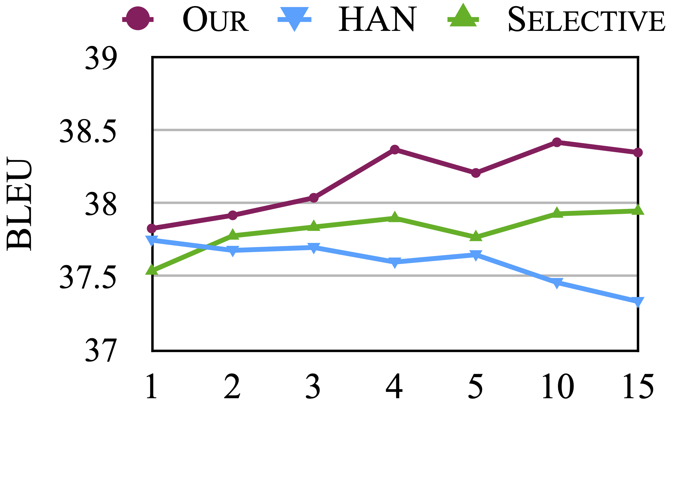
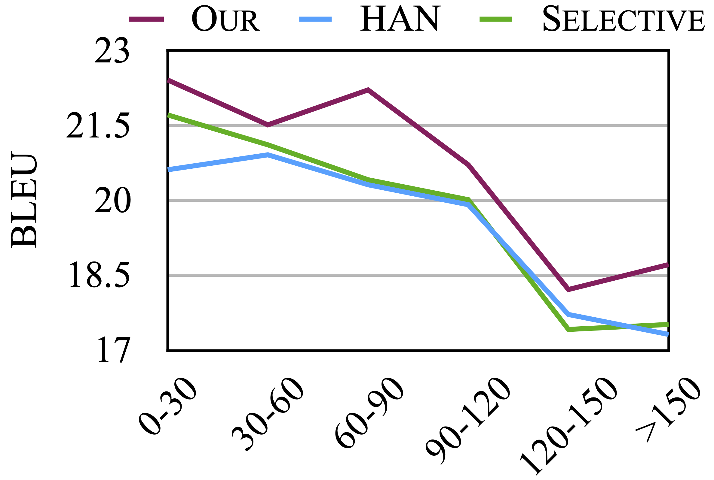
Figure 4a shows the influence of context distance on translation quality. We found that HAN performs worse when increasing the number of context sentences. One possible reason is that sequential structures introduce not only long-distance context but also more irrelevant information. By contrast, our model is getting better while more context is considered. This suggests that graphs help the model focus on relevant contexts regardless of their distance. Selective achieves a lower performance than our model and the gap becomes larger when on longer context, which we surmise is because the attention mechanism has difficulties to differentiate the usefulness of context. This also indicates that the prior knowledge indeed benefits to select relevant context.
Figure 4b shows evaluation results on different document lengths, i.e., the number of sentences in the document. We found that models considering global context (Selective and Our) achieve better results than HAN. Our is consistently better than Selective as well, especially on shorter and longer documents. These results suggest that a global context is beneficial to document-level NMT and appropriate consideration of global context is essential.
4.2 Influence of Dependency-Tree Accuracy
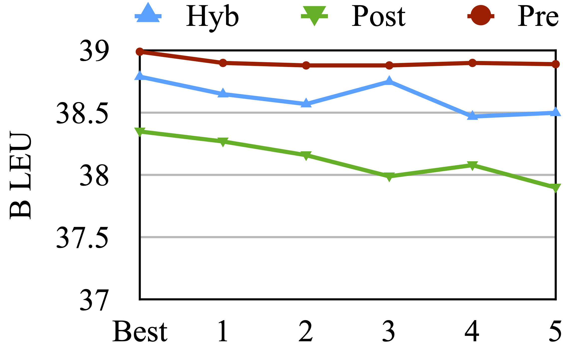
Figure 5 illustrates the influence of accuracy of dependency trees during inference. The Best means the best result from the dependency parser. The 1 to 5 denote dependency trees converted from the 5-best constituency trees of decreasing accuracy.555The version of the universal dependency parser in Stanford CoreNLP we used does not support generating n-best results. Therefore, we convert n-best constituent trees into dependency trees. We find that the performance of our systems with Post and Hyb methods slightly decrease when parsing accuracy becomes lower. However, the Pre method is more robust to parsing accuracy. We attribute this to the fact that integrating the document graph before the encoder leads to more opportunities to resist the noise.
| Model | Consistency | Discourse | |||
|---|---|---|---|---|---|
| Dex. | Lex. | Ell. | Coref. | Cohe. | |
| Base | |||||
| Noise | |||||
| HAN | |||||
| Selective | |||||
| Our | 77.3 | 72.5 | 75.1 | 69.5 | 58.5 |
| \hdashlinew/o tgt-g | |||||
| w/o Intra | |||||
| w/o Inter | |||||
4.3 Discourse Phenomena
We also examine whether our approaches are beneficial to capture discourse phenomena by evaluating our model on the Consistency test set Voita et al. (2019a) and Discourse test set Bawden et al. (2018).666More detailed reports on these tasks are presented in the Supplementary.
Test set
The Consistency test set contains three types of tasks on En–Ru: 1) Dex. checks the translation of deictic words or phrases. 2) Lex. focuses on the translation consistency of reiterative phrases. 3) Ell. tests whether models correctly predict ellipsis verb phrases or the morphology of words.
The Discourse test set consists of two probing tasks on En–Fr: 1) Coref. aims to test whether the gender of an anaphoric pronoun (it or they) is coherent with the previous sentence. 2) Cohe. is a set of ambiguous examples whose correct translations rely on the context.
Result on Discourse Phenomena
As shown in Table 5, all the context-aware models comprehensively improve the performance on discourse phenomena over the context-agnostic Base model. Results on the the Noise model Li et al. (2020) indicate that the improvement is not merely because of robust training. Compared to prior context-aware models, our model achieves the best accuracy on all tasks. Especially on the Lex., Coref. and Cohe. tasks, our model outperforms others over two points. Note that on the ellipsis task graph edges are usually missing for elided verb phrases. For example, given the following source sentence and its context Voita et al. (2019b), the verbs “told” and “did” are not directly connected in our graph but indirectly connected via the coreference relation of their neighbors “Nick” and “he”. Hence, our approach is still slightly better than the best prior method Selective. Directly linking such words may bring further improvements, which we leave for future work.
| Context | Nick told you what happened, right? |
|---|---|
| Source | Yeah, he did. |
Analysis on Graphs
We further conduct experiments with the hope of figuring out the influence of graphs on the discourse phenomena, as shown in Table 5. We found that our model with only source graphs (i.e., w/o TGT-G) is consistently better than the Base model on all tasks. Target graphs further improve it to achieve the best performance indicating the importance of target graphs on document-level translation. Both types of relations, Inter and Intra, make significant contributions as well. Their combination brings significant improvement verifying they are complementary to some extent. We also found that compared to Intra relations, Inter relations contribute more on all tasks except the Ell. task. We attribute this to the fact that our document graph contains inter-sentential relations, i.e., lexical consistency and coreference, which directly link relevant contexts for reiterative and deictic words.
| Model | Position | Sentence |
|---|---|---|
| SRC | 让我们叫他米格尔。 其实他的名字就是米格尔 | |
| 我一致在脑海中想象类似【帝企鹅日记】的事,我看着米格尔 | ||
| 我说,"米格尔,它们飞行150英里来渔场,然后它们晚上再飞150英里回去吗?" | ||
| REF | let’s call him miguel. his name is miguel. | |
| i was imagining a "march of the penguins" thing, so i looked at miguel. | ||
| i said, "miguel, do they fly 150 miles to the farm, and then do they fly 150 miles back at night? | ||
| Base | let’s call him migoa. his name is migoingle. | |
| i’ve always imagined something like a sekhri penguins’ diary, and i looked at igel. | ||
| i said, "miger, are they flying 150 miles to fishery, and then they fly 150 miles back at night?" | ||
| HAN | let’s call him migoa. his name is migoingle. | |
| i’ve been thinking about this like ’the penguins diary’ in my mind, and i’m looking at miger. | ||
| i said, miger, they fly 150 miles to fisheries, and they fly 150 miles at night? | ||
| OUR | let’s call him migel. his name is migel. | |
| and i’ve always imagined something like a ’timend penguin diary’ in my head, and i’m looking at migel. | ||
| and i said, "migel, they fly 150 miles to fisheries, and then they fly 150 miles back at night? |
4.4 Case-Study
To verify the long-distance consistency, we perform case studies on the Zh–En task. Table 6 shows an example where a named entity “米格尔” (miguel) repeatedly appears in different positions in the document. We first found that both document-level NMT systems, i.e., HAN and Our, generate more consistent translations of the entity than the context-agnostic Base model. Compared with the HAN model, Our system keeps translating “米格尔” into “migel”, suggesting a more effective capability of handling consistency in long-distance context.
5 Related work
In recent years, a variety of studies work on improving document-level machine translation with context. Most of them focus on using a limited number of previous sentences. One typical approach is to equip conventional sentence-level NMT with an additional encoder to learn context representations, which are then integrated into encoder and/or decoder (Jean et al., 2015; Zhang et al., 2018; Voita et al., 2018). Wang et al. Wang et al. (2017) and Miculicich et al. Miculicich et al. (2018) adopted hierarchical mechanisms to integrate contexts into NMT models. Tu et al. Tu et al. (2018) and Kuang et al. Kuang et al. (2018) used cache-based methods to memorize historical translations which are then used in following decoding steps.
Recently, several studies have endeavoured to consider the full document context. Macé and Servan Macé and Servan (2019) averaged the word embeddings of a document to serve as the global context directly. Maruf and Haffari Maruf and Haffari (2018) applied a memory network to remember hidden states of the document, which are then attended by a decoder. Maruf et al. Maruf et al. (2019) first selected relevant sentences as contexts and then attended to words in these sentences. Tan et al. Tan et al. (2019) learned global context-aware representations by firstly using a sentence encoder followed by a document encoder. Junczys-Dowmunt Junczys-Dowmunt (2019) considered the global context by merely concatenating all the sentences in a document. Zheng et al. (2020) took an additional attention layer to get a representation mixed from the current sentence and whole document. Kang et al. (2020) dynamically selected the relevant context from the whole document via a reinforcement learning method.
Unlike previous approaches, we represent document-level global context in graph encoded by graph encoders and integrated into conventional NMT via attention and gating mechanisms.
6 Conclusion
In this paper, we propose a graph-based approach for document-level translation, which leverages both source and target contexts. Graphs are constructed according to inter-sentential and intra-sentential relations. We employ a GCN-based graph encoder to learn the graph representations, which are then fed into the NMT model via attention and gating mechanisms. Experiments on four translation tasks and several existing architectures show the proposed approach consistently improves translation quality across different language pairs. Further analyses demonstrate the effectiveness of graphs and the capability of leveraging long-distance context. In the future, we would like to enrich the types of relations to cover more document phenomena.
Acknowledgements
This work was supported in part by the Science and Technology Development Fund, Macau SAR (Grant No. 0101/2019/A2), and the Multi-year Research Grant from the University of Macau (Grant No. MYRG2020-00054-FST).
References
- Bastings et al. (2017) Joost Bastings, Ivan Titov, Wilker Aziz, Diego Marcheggiani, and Khalil Sima’an. 2017. Graph convolutional encoders for syntax-aware neural machine translation. In ACL.
- Bawden et al. (2018) Rachel Bawden, Rico Sennrich, Alexandra Birch, and Barry Haddow. 2018. Evaluating Discourse Phenomena in Neural Machine Translation. In NAACL.
- Cettolo et al. (2012) Mauro Cettolo, Christian Girardi, and Marcello Federico. 2012. Wit3: Web inventory of transcribed and translated talks. In EAMT.
- Huang et al. (2020) Luyang Huang, Lingfei Wu, and Lu Wang. 2020. Knowledge graph-augmented abstractive summarization with semantic-driven cloze reward. In ACL.
- Jean et al. (2015) Sébastien Jean, Kyunghyun Cho, Roland Memisevic, and Yoshua Bengio. 2015. On Using Very Large Target Vocabulary for Neural Machine Translation. In ACL.
- Junczys-Dowmunt (2019) Marcin Junczys-Dowmunt. 2019. Microsoft translator at wmt 2019: Towards large-scale document-level neural machine translation. In WMT.
- Kang et al. (2020) Xiaomian Kang, Yang Zhao, Jiajun Zhang, and Chengqing Zong. 2020. Dynamic Context Selection for Document-level Neural Machine Translation via Reinforcement Learning. In EMNLP.
- Kim et al. (2019) Yunsu Kim, Duc Thanh Tran, and Hermann Ney. 2019. When and Why is Document-level Context Useful in Neural Machine Translation? In DiscoMT.
- Koehn (2004) Philipp Koehn. 2004. Statistical significance tests for machine translation evaluation. In EMNLP.
- Koncel-Kedziorski et al. (2019) Rik Koncel-Kedziorski, Dhanush Bekal, Yi Luan, Mirella Lapata, and Hannaneh Hajishirzi. 2019. Text generation from knowledge graphs with graph transformers. In NAACL.
- Kuang et al. (2018) Shaohui Kuang, Deyi Xiong, Weihua Luo, and Guodong Zhou. 2018. Modeling Coherence for Neural Machine Translation with Dynamic and Topic Caches. In Coling.
- Läubli et al. (2018) Samuel Läubli, Rico Sennrich, and Martin Volk. 2018. Has Machine Translation Achieved Human Parity? A Case for Document-level Evaluation. In EMNLP.
- Li et al. (2020) Bei Li, Hui Liu, Ziyang Wang, Yufan Jiang, Tong Xiao, Jingbo Zhu, Tongran Liu, and Changliang Li. 2020. Does Multi-Encoder Help? A Case Study on Context-Aware Neural Machine Translation. ACL.
- Lin et al. (2019) Peiqin Lin, Meng Yang, and Jianhuang Lai. 2019. Deep mask memory network with semantic dependency and context moment for aspect level sentiment classification. In IJCAI.
- Ma et al. (2020) Shuming Ma, Dongdong Zhang, and Ming Zhou. 2020. A Simple and Effective Unified Encoder for Document-Level Machine Translation. In ACL.
- Macé and Servan (2019) Valentin Macé and Christophe Servan. 2019. Using whole document context in neural machine translation. In IWSLT.
- Marcheggiani and Titov (2017) Diego Marcheggiani and Ivan Titov. 2017. Encoding sentences with graph convolutional networks for semantic role labeling. In EMNLP.
- Maruf and Haffari (2018) Sameen Maruf and Gholamreza Haffari. 2018. Document Context Neural Machine Translation with Memory Networks. In ACL.
- Maruf et al. (2019) Sameen Maruf, André FT Martins, and Gholamreza Haffari. 2019. Selective Attention for Context-aware Neural Machine Translation. In NAACL.
- Miculicich et al. (2018) Lesly Miculicich, Dhananjay Ram, Nikolaos Pappas, and James Henderson. 2018. Document-Level Neural Machine Translation with Hierarchical Attention Networks. In EMNLP.
- Ott et al. (2019) Myle Ott, Sergey Edunov, Alexei Baevski, Angela Fan, Sam Gross, Nathan Ng, David Grangier, and Michael Auli. 2019. fairseq: A Fast, Extensible Toolkit for Sequence Modeling. In NAACL-HLT.
- Papineni et al. (2002) Kishore Papineni, Salim Roukos, Todd Ward, and Wei-Jing Zhu. 2002. BLEU: A Method for Automatic Evaluation of Machine Translation. In ACL.
- Scherrer et al. (2019) Yves Scherrer, Jörg Tiedemann, and Sharid Loáiciga. 2019. Analysing Concatenation Approaches to Document-Level NMT in Two Different Domains. In DiscoMT 2019.
- Sennrich et al. (2016) Rico Sennrich, Barry Haddow, and Alexandra Birch. 2016. Neural Machine Translation of Rare Words with Subword Units. In ACL.
- Strubell et al. (2018) Emma Strubell, Patrick Verga, Daniel Andor, David Weiss, and Andrew McCallum. 2018. Linguistically-informed self-attention for semantic role labeling. In EMNLP.
- Tan et al. (2019) Xin Tan, Longyin Zhang, Deyi Xiong, and Guodong Zhou. 2019. Hierarchical Modeling of Global Context for Document-Level Neural Machine Translation. In EMNLP-IJCNLP.
- Tiedemann and Scherrer (2017) Jörg Tiedemann and Yves Scherrer. 2017. Neural Machine Translation with Extended Context. In DiscoMT.
- Tu et al. (2018) Zhaopeng Tu, Yang Liu, Shuming Shi, and Tong Zhang. 2018. Learning to remember translation history with a continuous cache. In TACL.
- Vaswani et al. (2017) Ashish Vaswani, Noam Shazeer, Niki Parmar, Jakob Uszkoreit, Llion Jones, Aidan N Gomez, Łukasz Kaiser, and Illia Polosukhin. 2017. Attention Is All You Need. In NISP.
- Voita et al. (2019a) Elena Voita, Rico Sennrich, and Ivan Titov. 2019a. Context-Aware Monolingual Repair for Neural Machine Translation. In EMNLP.
- Voita et al. (2019b) Elena Voita, Rico Sennrich, and Ivan Titov. 2019b. When a Good Translation is Wrong in Context: Context-Aware Machine Translation Improves on Deixis, Ellipsis, and Lexical Cohesion. In ACL.
- Voita et al. (2018) Elena Voita, Pavel Serdyukov, Rico Sennrich, and Ivan Titov. 2018. Context-Aware Neural Machine Translation Learns Anaphora Resolution. In ACL.
- Wang et al. (2017) Longyue Wang, Zhaopeng Tu, Andy Way, and Qun Liu. 2017. Exploiting Cross-Sentence Context for Neural Machine Translation. In EMNLP.
- Xu et al. (2019) Mingzhou Xu, Derek F Wong, Baosong Yang, Yue Zhang, and Lidia S Chao. 2019. Leveraging local and global patterns for self-attention networks. In ACL2019.
- Yang et al. (2018) Baosong Yang, Zhaopeng Tu, Derek F Wong, Fandong Meng, Lidia S Chao, and Tong Zhang. 2018. Modeling Localness for Self-Attention Networks. In EMNLP.
- Yang et al. (2019) Zhengxin Yang, Jinchao Zhang, Fandong Meng, Shuhao Gu, Yang Feng, and Jie Zhou. 2019. Enhancing Context Modeling with a Query-Guided Capsule Network for Document-level Translation. In EMNLP-IJCNLP.
- Zhang et al. (2019) Biao Zhang, Ivan Titov, and Rico Sennrich. 2019. Improving Deep Transformer with Depth-Scaled Initialization and Merged Attention. In EMNLP-IJCNLP.
- Zhang et al. (2018) Jiacheng Zhang, Huanbo Luan, Maosong Sun, Feifei Zhai, Jingfang Xu, Min Zhang, and Yang Liu. 2018. Improving the Transformer Translation Model with Document-Level Context. In EMNLP.
- Zheng et al. (2020) Zaixiang Zheng, Xiang Yue, Shujian Huang, Jiajun Chen, and Alexandra Birch. 2020. Towards Making the Most of Context in Neural Machine Translation. In IJCAI.
Appendix A Experiments
| Benchmark | Language | Sent–level | Doc–level | Development | testing | |||
|---|---|---|---|---|---|---|---|---|
| Doc. | Sent. | Doc. | Sent. | Doc. | Sent. | |||
| IWSLT 777(https://wit3.fbk.eu/) | En–Fr | – | K | |||||
| Zh–En | – | K | ||||||
| Opensubtitle888https://github.com/lena-voita/good-translation-wrong-in-context | En–Ru | M | M | M | K | K | K | K |
| WMT999https://github.com/Helsinki-NLP/doclevel-MT-benchmark | En–De | M | M | |||||
Data
The statistics of the datasets are reported in Table 7. For the Chinese language, we segment the data set with the jieba toolkit but the Moses tokenizer.pl for the other languages. WMT19 and Opensubtitle are will pre-processed by Scherrer et al. (2019) and Voita et al. (2018).
| Aggregation | BLEU |
|---|---|
| Gating Units | |
| Attention |
| #Layers | Shared | BLEU |
|---|---|---|
| 1 | – | |
| 2 | – | |
| 2 | Share | |
| 3 | – |
| Ablation | Model | Dev | Test |
|---|---|---|---|
| Base | |||
| +TF-IDF | |||
| +All |
| Ablation | Model | Dev | Test |
|---|---|---|---|
| Src-graph | |||
| Tgt-graph | |||
| Both |
Settings
We incorporate the proposed approach into the widely used context-agnostic framework Transformer (Vaswani et al., 2017) on Fairseq toolkit Ott et al. (2019). The model are trained on V100 GPU. The conventional context-agnostic Transformer models are trained with BASE settings. For the IWSLT and Opensubtitle benchmarks, we train the context-agnostic model with 0.2 dropout. The learning rate is set to 0.0007 with 4k warm-up steps. We set the dropout of the document graph encoder to 0.2, which tuned on validation set. We use approximately 16,000 tokens in a mini-batch for En-Fr, Zh-En, En-Ru, and 32,000 for En–De.
Appendix B Ablation Study
Graph Encoder
We extend the GCN-based graph encoder with an attention mechanism to combine different representations, which is different from the gate-based method in previous work (Bastings et al., 2017). Table 8 shows that the attention-based aggregation works better in our model. We presume this is because the attention mechanism balances the contributions of different representations. Table 9 shows the influence of the graph encoder with various numbers of layers. We found that stacking two graph encoder layers and sharing their parameter obtains the best performance. Further increasing the number of layers does not lead improvement. This finding is consistent with existing works as well (Marcheggiani and Titov, 2017; Bastings et al., 2017). As shown in Table 10, we also investigate the traditional TF-IDF construction method, the result indicates that our method is not limited to the examined relations but also works with other graph construction methods.
Graph Contribution
We evaluated the performance of the context form each side. As seen in Table 11, only using the source or target side graph shows comparable performance. With both source and target context further improve the translation quality.
B.1 Discourse Phenomena
Test set
The consistency test set Voita et al. (2019b) contains four tasks on En–Ru: 1) Deixis aims to detect the deictic words or phrases whose denotation depends on the context. 2) Lex.C is a lexical cohesion task, which focuses on the reiteration of named entities. 3) Ell.inf tests the model on words whose morphological form depends on the context. 4) Ell.VP is to test whether the model can correctly predict the ellipsis verb phrase in Russian. Discourse test set Bawden et al. (2018) consists of two probing tasks on En–Fr: 1) Coref. aims to test the anaphoric pronoun (it or they) whose gender is coherent with the previous sentence. 2) Coh. is a set of ambiguous examples whose correct translations rely on the context. The difference between the Cor. and Sem. is whether the context is correct or not.
| Model | Deixis | Lex.C | Ell.inf | Ell.VP |
|---|---|---|---|---|
| Base | ||||
| Noise | ||||
| Ctx | ||||
| Unified | ||||
| HAN | ||||
| Selective | 74.6 | |||
| Post | ||||
| Pre | 77.9 | 74.8 | ||
| Hyb. | 76.3 | |||
| \hdashlinew/o tgt-g | ||||
| w/o Intra | ||||
| w/o Inter |
| Model | Coref.() | Coh.() | ||
|---|---|---|---|---|
| ALL | Cor. | Sem. | ALL | |
| Base | ||||
| Noise | ||||
| Ctx | ||||
| Unified | ||||
| HAN | ||||
| Selective | ||||
| Post. | ||||
| Pre | 69.5 | 73.0 | 59.5 | |
| Hyb. | 69.5 | 68.5 | ||
| \hdashlinew/o tgt-g | ||||
| w/o Intra | ||||
| w/o Inter | ||||