Learning Graph Neural Networks with Approximate Gradient Descent

Abstract

The first provably efficient algorithm for learning graph neural networks (GNNs) with one hidden layer for node information convolution is provided in this paper. Two types of GNNs are investigated, depending on whether labels are attached to nodes or graphs. A comprehensive framework for designing and analyzing convergence of GNN training algorithms is developed. The algorithm proposed is applicable to a wide range of activation functions including ReLU, Leaky ReLU, Sigmod, Softplus and Swish. It is shown that the proposed algorithm guarantees a linear convergence rate to the underlying true parameters of GNNs. For both types of GNNs, sample complexity in terms of the number of nodes or the number of graphs is characterized. The impact of feature dimension and GNN structure on the convergence rate is also theoretically characterized. Numerical experiments are further provided to validate our theoretical analysis.

Introduction

Recent success of deep neural network (DNN) has dramatically boosted its application in various application domains, e.g., computer vision (Krizhevsky, Sutskever, and Hinton 2012), natural language processing (Young et al. 2018) and strategic reasoning with reinforcement learning (Sutton and Barto 2018; Silver et al. 2017). Although DNN usually has millions of parameters and a highly non-convex objective function, simple optimization techniques, e.g., stochastic gradient descent and its variants, can efficiently train such a complicated structure successfully. However, there are many applications, where data is represented in the form of graphs. For example, in social networks, a graph-based learning system can exploit the interconnection between the users to make highly accurate inferences. DNN, when applied to graph based structural data, has to face with some new challenges, and cannot be directly applied. To address the new challenges, graph neural network (GNN) has been proposed recently and has been demonstrated to have massive expressive power on graphs. GNNs have been shown to be successful in many application domains, e.g., social networks, knowledge graph, recommender systems, molecular fingerprint, and protein interface networks (Wu et al. 2019; Xu et al. 2018; Zhou et al. 2018).

Although being successful in practical applications, theoretical understanding of GNNs is still lacking in the literature. There is a strong need to theoretically understand why GNNs work well on practical graph-structured data, and to further design provably efficient learning algorithms for GNN.

However, even for commonly used DNN architectures, it is in general challenging to develop theoretical understanding of the learning dynamics and to learn simple neural networks (Goel, Klivans, and Meka 2018). Specifically, if we assume that the data is generated according to a teacher neural network, the goal is then to recover the true parameters of the teacher neural network. The major challenge lies in the highly non-convex nature of DNN’s objective function. For example, in the agnostic setting with bounded distributions and square loss, learning a single ReLU with unit norm hidden weight vectors is notoriously difficult (Goel et al. 2017). It was proved by Brutzkus and Globerson (Gautier, Nguyen, and Hein 2016) that the problem of distribution-free recover of the unknown weight vector for learning one hidden layer convolutional neural network (CNN) is NP-hard, even if non-overlapping patch structure is assumed. At this point, a major open problem is still to understand mildest conditions and design of provably efficient algorithms that lead to learnability of neural networks in polynomial time.

In this paper, we focus on the parameter recovery problem for learning GNNs where the training data is generated according to a teacher GNN. We design provably efficient algorithms to recover the true parameters of the teacher GNN. Our focus is to develop a comprehensive framework for designing and analyzing convergence of GNN training algorithms.

Main Contributions

Our first contribution is the design and convergence analysis of an approximate gradient descent algorithm for training GNNs. The algorithm is based on the idea of inexact optimization and approximate training (Schmidt, Roux, and Bach 2011; Li et al. 2017; Cao and Gu 2019), and the major advantage is that it reduces computational complexity while guaranteeing convergence and learnability at the same time. We prove that the proposed algorithm recovers the underlying true parameters of the teacher network with a linear convergence rate up to statistical precision. The assumptions are mild, and can be easily satisfied in practice. Specifically, our analysis is applicable to a wide range of activation functions (see Assumptions 1 and 2), e.g., ReLU, Leaky ReLU, Sigmod, Softplus and Swish. The analysis only requires that the activation functions to be monotonic increasing, and Lipschitz, and does not depend on the specific gradient computation involved in the activation function (Brutzkus and Globerson 2017; Du, Lee, and Tian 2017; Safran and Shamir 2018).

Our second contribution is the introduction and the extension of the technique of approximate calculation in gradients for the algorithm in order to analyze GNNs. A similar idea was first proposed in (Cao and Gu 2019) to analyze the learnability of CNNs with non-overlapping convolution patches. We highlight that the non-overlapping convolution process is very different from the nature that the feature convolution at nodes in GNNs is intrinsically overlapping, as nodes may share common neighbors. The analysis framework in (Cao and Gu 2019) cannot be directly applied in GNN analysis. We extend the scope of the methodology and propose provably efficient algorithms to learn and analyze GNNs.

Our third contribution is that we investigate the empirical version of the problem where the estimation of parameters is based on $n$ independent samples. We provide uniform convergence results of the proposed algorithm with respect to the sample complexity. We also provide the parameter training dynamics with the proposed algorithm, and show that the training is provably stable.

To the best of the authors’ knowledge, these theoretical results are the first sharp analyses of statistical efficiency of GNNs. For ease of presentation, we hereby informally present the main theorem in the paper as follows. We refer readers to Theorem 2 for the precise statements.

Theorem 1 (Main Theorem (Informal)).

GNN is stably learnable with the proposed algorithms in linear time.

Related Work

There is a recent surge of interest in theoretically understanding properties of DNNs, e.g., hardness of learning (Goel et al. 2017; Song et al. 2017), landscape of neural networks (Kawaguchi 2016; Choromanska et al. 2015; Hardt and Ma 2016; Haeffele and Vidal 2015; Freeman and Estrach 2019; Safran and Shamir 2016; Zhou and Feng 2017; Nguyen and Hein 2017b, a; Ge, Lee, and Ma 2017; Safran and Shamir 2018; Du and Lee 2018), training dynamics using gradient descent approaches (Tian 2017; Zhong et al. 2017; Li and Yuan 2017; Du et al. 2018), and design of provable learning algorithms (Goel and Klivans 2017a, b; Zhang et al. 2015). For non-convex optimization problems that satisfy strict saddle property, it was shown in (Du, Lee, and Tian 2017) and (Jin et al. 2017) that (stochastic) gradient descent converges in polynomial time. The landscape of neural networks were then extensively studied (Soltanolkotabi 2017; Kawaguchi 2016; Choromanska et al. 2015; Hardt and Ma 2016; Haeffele and Vidal 2015; Freeman and Estrach 2019; Safran and Shamir 2016; Zhou and Feng 2017; Nguyen and Hein 2017b, a; Ge, Lee, and Ma 2017; Safran and Shamir 2018; Du and Lee 2018). Specifically, algorithms were designed for specific neural network architectures, and their learning of a neural network in polynomial time and sample complexity were further characterized (Goel et al. 2017; Zhang, Lee, and Jordan 2016; Zhang et al. 2015; Sedghi and Anandkumar 2014; Janzamin, Sedghi, and Anandkumar 2015; Gautier, Nguyen, and Hein 2016; Goel and Klivans 2017b; Du, Lee, and Tian 2017).

However, to the best of our knowledge, there has been no related attempt to understand the training dynamics and to design provably efficient learning algorithms for GNNs. In recent advances (Du, Lee, and Tian 2017; Du et al. 2017; Goel, Klivans, and Meka 2018; Brutzkus and Globerson 2017; Zhong, Song, and Dhillon 2017), the condition for (stochastic) gradient descent or its variants to recover the underlying true parameter under the teacher-student model in polynomial time were analyzed for CNNs. Specifically, for spherical Gaussian distribution and non-overlapping patch structures, gradient descent approach can recover the underlying true parameter in polynomial time for CNNs (Brutzkus and Globerson 2017; Du et al. 2017). In (Cao and Gu 2019), the information theoretic limits and the computational complexity of learning a CNN were developed.

Note that the GNN shares a similar convolutional structure as the CNN (LeCun, Bengio et al. 1995), and is therefore closely related to the CNN. Specifically, an image can be viewed as a graph grid where adjacent pixels are connected by edges. Similar to a 2D convolution for an image, graph convolution can also be performed on an image by taking an weighted average of information from adjacent pixels. Here, each pixel in an image can be viewed as a node in a graph, and its neighbors are ordered. The size of neighbors are then determined by the convolution filer size. However, different from image data, the neighbors of a node in a graph for GNNs are unordered, and vary in sizes. Moreover, information convolution in graph is by nature overlapping. Therefore, the analysis for CNNs is intrinsically different from and cannot be directly carried over to the analysis for GNNs. We will elaborate this in this paper.

Notations

Let $\left\lVert\cdot\right\rVert_{2}$ denote the Euclidean norm of a finite-dimensional vector or a matrix. For a positive semidefinite matrix $X$, we use $\sigma_{m}(X)$ as its nonzero smallest eigenvalue and $\sigma_{M}(X)$ as its nonzero largest eigenvalue in sequel. Throughout this paper, we use capital letters to denote matrices, lower case letters to denote vectors, and lower case Greek letters to denote scalars. We denote $x\wedge y\triangleq\min\{x,y\}$.

The Graph Neural Network

In this section, we formalize the GNN model with one layer of node information convolution.

Node-level GNN (NGNN) with One Graph

We first investigate one graph with $n$ nodes, and node $i$ has a feature $\mathbf{H}_{i}\in\mathbb{R}^{d}$ with dimension $d$. We define $\mathbf{H}\in\mathbb{R}^{n\times d}$ as the node feature matrix of the graph. To learn a GNN, a node first collects all the features from its neighboring nodes, and updates its own feature with a shared local transition function among these nodes. This process is termed as graph convolution and can be expressed as

$$\hat{\mathbf{H}}_{i}=\sigma\left(\frac{1}{\left|\mathcal{N}_{i}\right|}\sum_{j\in\mathcal{N}_{i}}\mathbf{H}_{j}\mathbf{W}\right),$$ (1)

where $\sigma$ is the activation function, $\mathcal{N}_{i}$ is the set containing node $i$ and all its neighboring nodes, and $\mathbf{W}\in\mathbb{R}^{d\times d_{out}}$ represents the local transition function which usually is a fully connected network taking in the averaged node feature and outputs the updated feature. After this process, the node feature gets updated with a change in dimension from $d$ to $d_{out}$. The above process of graph convolution can be written in a global point of view as

$$\hat{\mathbf{H}}=\sigma(\mathbf{D}^{-1}\mathbf{A}\mathbf{H}\mathbf{W}),$$ (2)

where $\mathbf{D}\in\mathbb{R}^{n\times n}$ is the degree matrix of the graph and $\mathbf{A}\in\mathbb{R}^{n\times n}$ is the corresponding adjacency matrix. Here, $\mathbf{D}^{-1}\mathbf{A}\mathbf{H}$ is the operation that one node updates its feature by taking the average of its own features and features of its neighbors.

After the graph convolution, each node has its own feature updated, by incorporating local structural information of the graph and features from its neighboring nodes. Then, the updated node feature is passed into a fully connected layer $\mathbf{v}\in\mathbb{R}^{d_{out}}$. Thus, the output of the entire graph neural network for node-level tasks is

$$\hat{\mathbf{y}}=\sigma(\mathbf{D}^{-1}\mathbf{A}\mathbf{H}\mathbf{W})\mathbf{v}\in\mathbb{R}^{n}.$$ (3)

As we have one graph, suppose the graph has a node-level label vector $\mathbf{y}\in\mathbb{R}^{n}$, and we have $n$ ground truth data pairs $\{\mathbf{H}_{i},\mathbf{y}_{i}\}_{i=1}^{n}$. We assume that the node feature matrix $\mathbf{H}\in\mathbb{R}^{n\times d}$ is generated independently from the standard Gaussian distribution, and the corresponding output $\mathbf{y}\in\mathbb{R}^{n}$ is generated from the teacher network with true parameters $\mathbf{W}^{\ast}$ and $\mathbf{v}^{\ast}$ as follows

$$\mathbf{y}=\sigma(\mathbf{D}^{-1}\mathbf{A}\mathbf{H}\mathbf{W}_{\ast})\mathbf{v}_{\ast}+\epsilon.$$ (4)

Here, $\{\epsilon_{i}\}_{i=1}^{n}$ are independent sub-Gaussian white noises with $\psi_{2}$ norm $\nu$, which is a broader class including Gaussian noise but far less restrictive. Without loss of generality, we assume that $\|\mathbf{W}_{\ast}\|_{2}=1$ in this paper.

Graph-level GNN (GGNN) with Multiple Graphs

We then investigate with $n$ graphs, and the $j$-th graph has $n_{j}$ nodes with the node feature matrix $\mathbf{H}_{j}\in\mathbb{R}^{n_{j}\times d}$. Similar to the convolution for the case of one graph for NGNN, the $j$-th graph updates its node features by the following convolution process

$$\hat{\mathbf{H}}_{j}=\sigma(\mathbf{D}_{j}^{-1}\mathbf{A}_{j}\mathbf{H}_{j}\mathbf{W}),$$ (5)

where $\sigma$ is the activation function, $\mathbf{D}_{j}\in\mathbb{R}^{n_{j}\times n_{j}}$ is the degree matrix of $j$-th graph, and $\mathbf{A}_{j}\in\mathbb{R}^{n_{j}\times n_{j}}$ is the corresponding adjacency matrix. Here, $\mathbf{D}_{j}^{-1}\mathbf{A}_{j}\mathbf{H}_{j}$ is the operation that one node in the $j$-th graph updates its feature by taking the average of its own features and the features of its neighbors. $\mathbf{W}\in\mathbb{R}^{d\times d_{out}}$ represents the local transition function which is shared among different nodes across different graphs.

For GGNN, graph $j$ with $n_{j}$ node features has to aggregate the node features such that the graph has a unique graph-level representation. In the following, we discuss several aggregation methods which are most widely used in the literature.

Particular node feature as graph embedding. This method picks a specific node feature to represent the global graph embedding. Define $\mathbf{g}_{j}\in R^{d}$ as the embedding for the $j$-th graph, which in this case is expressed as

$$\mathbf{g}_{j}^{T}=\mathbf{a}_{j}\sigma(\mathbf{D}_{j}^{-1}\mathbf{A}_{j}\mathbf{H}_{j}\mathbf{W}),$$ (6)

where $\mathbf{a}_{j}\in R^{1\times n_{j}}$ is a row vector with “1” as its $i$-th element and otherwise “0”. Consequently, the $i$-th node feature is picked to represent the $j$-th graph for follow-up graph-level tasks.

Attention-based Aggregation. In this approach, the graph embedding is a weighted sum of the node features and the weight is usually termed as attention that is learned from the corresponding node feature. The attention-based weighted feature aggregation for the $j$-th graph can be expressed as

$$\mathbf{g}_{j}^{T}=\mathbf{a}_{j}\sigma(\mathbf{D}_{j}^{-1}\mathbf{A}_{j}\mathbf{H}_{j}\mathbf{W}),$$ (7)

where $\mathbf{a}_{j}\in R_{+}^{1\times n_{j}}$ is an attention row vector for all the nodes, with non-negative elements summing up to 1.

Averaging. Averaging is a special case of the attention based aggregation where the attention is identical for all the node features. Thus, we can write

$$\mathbf{g}_{j}^{T}=\frac{1}{n_{j}}\mathbf{1}_{n_{j}}\sigma(\mathbf{D}_{j}^{-1}\mathbf{A}_{j}\mathbf{H}_{j}\mathbf{W}),$$ (8)

where $\mathbf{1}_{n_{j}}$ is a $n_{j}$ dimensional row vector of all ones.

After the graph convolution and the node feature aggregation, each graph has its own embedding, incorporating its local structural information and all its node features. Then, the graph embedding is passed into a fully connected layer $\mathbf{v}\in\mathbb{R}^{d}$. Thus, the output of the $j$-th graph for graph-level tasks is

$$\hat{y}_{j}=\mathbf{a}_{j}\sigma(\mathbf{D}_{j}^{-1}\mathbf{A}_{j}\mathbf{H}_{j}\mathbf{W})\mathbf{v}\in\mathbb{R}.$$ (9)

As we have multiple graphs, suppose each graph has a graph-level label $y_{j}\in\mathbb{R}$, and we have $n$ ground truth data pairs $\{\mathbf{H}_{j},y_{j}\}_{j=1}^{n}$. We assume that each node feature matrix $\mathbf{H}_{j}\in\mathbb{R}^{n_{j}\times d}$ is generated independently from the standard Gaussian distribution, and the corresponding output $y_{j}\in\mathbb{R}$ is generated from the teacher network with true parameters $\mathbf{W}^{\ast}$ and $\mathbf{v}^{\ast}$ as follows,

$$y_{j}=\mathbf{a}_{j}\sigma(\mathbf{D}_{j}^{-1}\mathbf{A}_{j}\mathbf{H}_{j}\mathbf{W}_{\ast})\mathbf{v}_{\ast}+\epsilon_{j}.$$ (10)

Here, $\{\epsilon_{j}\}_{j=1}^{n}$ are independent sub-Gaussian white noises with $\psi_{2}$ norm $\nu$. Through out this paper, we assume that $\|\mathbf{W}_{\ast}\|_{2}=1$. For simplicity, we assume that the learning process for $\mathbf{W}$ and $\mathbf{v}$ is disjoint from that for $\mathbf{a}_{j}$, or $\mathbf{a}_{j}$ is fixed and does not need training.

Assumptions

In this paper, we make the following assumptions, which can be easily satisfied with commonly used activation functions in practice, e.g., ReLU, Leaky ReLU, Sigmod and Softplus.

Assumption 1.

$\sigma$ is a non-trivial increasing function, and is 1-Lipschitz continuous, i.e., $\left|\sigma(x_{1})-\sigma(x_{2})\right|\leq\left|x_{1}-x_{2}\right|,\forall x_{1},x_{2}\in\mathbb{R}$.

Assumption 2.

$\left\lVert\sigma(x)\right\rVert_{2}\leq L_{\sigma}\left\lVert x\right\rVert_{2},\forall x\in\mathbb{R}^{n}$.

Algorithm and Main Results

We study the sample complexity and training dynamics of learning GNNs with one convolution layer. We construct novel algorithms for training GNNs, and further prove that, with high probability, the proposed algorithms with proper initialization and training step size grant a linear convergence to the ground-truth parameters up to statistical precision. Our results apply to general non-trivial, monotonic and Lipschitz continuous activation functions including ReLU, Leaky ReLU, Sigmod, Softplus and Swish.

Algorithm Design

We present the algorithm in Algorithm 1 for NGNN and GGNN with two auxiliary matrices defined as

$$\Xi_{N}=\operatorname{\mathbb{E}}\left[\mathbf{H}^{\top}\mathbf{A}^{\top}(\mathbf{D}^{-1})^{\top}\sigma(\mathbf{D}^{-1}\mathbf{A}\mathbf{H})\right],$$ (11)

and

$$\Xi_{G}=\frac{1}{n}\sum_{j=1}^{n}\operatorname{\mathbb{E}}\left[\mathbf{H}_{j}^{\top}\mathbf{A}_{j}^{\top}(\mathbf{D}_{j}^{-1})^{\top}\mathbf{a}_{j}^{\top}\mathbf{a}_{j}\sigma(\mathbf{D}_{j}^{-1}\mathbf{A}_{j}\mathbf{H}_{j})\right].$$ (12)

It is easy to see that the above two matrices are invertible under Assumption 1. For learning NGNN (similar for GGNN), if we replace $\Xi_{N}^{-1}$ by the gradient $\sigma^{\prime}\left(\mathbf{D}^{-1}\mathbf{A}\mathbf{H}\right)$, we have exact gradients for $\mathbf{W}$ and $\mathbf{v}$ with a square loss $\frac{1}{n}\left\lVert\mathbf{y}-\sigma(\mathbf{D}^{-1}\mathbf{A}\mathbf{H}\mathbf{W})\mathbf{v}\right\rVert_{2}^{2}$. However, calculating $\sigma^{\prime}\left(\mathbf{D}^{-1}\mathbf{A}\mathbf{H}\right)$ for some activation functions could be computationally expensive. Note that to compute these matrices of (11) and (12), one only needs to make an epoch pass on the dataset. Compared with a regular training by DNNs with tons of epoch passes on the entire dataset to acquire exact gradients, obtaining the two matrices adds very limited burden to the training computation. Hence, the gradient of $\mathbf{W}$ is inexact in the algorithm and a similar idea is also adopted in analysis of CNNs (Cao and Gu 2019).

Input: Training data $\{\mathbf{H},\mathbf{y}\}$, number of iterations $T$, step size $\alpha$, initialization $\mathbf{W}_{0},\mathbf{v}_{0},t=1$.

1 while $t<T$ do

2       $\bar{c}=\begin{cases}\mathbf{D}^{-1}\mathbf{A}\mathbf{H},&\text{NGNN},\\ \mathbf{D}_{j}^{-1}\mathbf{A}_{j}\mathbf{H}_{j},&\text{GGNN}.\end{cases}$

3      $\bar{y}=\begin{cases}\sigma(c^{\prime}\mathbf{W}_{t})\mathbf{v}_{t},&\text{NGNN},\\ \mathbf{a}_{j}\sigma(c^{\prime}\mathbf{W}_{t})\mathbf{v}_{t},&\text{GGNN}.\end{cases}$

4      $\mathbf{G}^{W}_{t}=\begin{cases}-\frac{1}{n}\Xi_{N}^{-1}\bar{c}^{\top}\left(\mathbf{y}-\bar{y}\right)\mathbf{v}_{t}^{\top},&\text{NGNN},\\ -\frac{1}{n}\Xi_{G}^{-1}\sum_{j=1}^{n}\bar{c}^{\top}\mathbf{a}_{j}^{\top}\left(y_{j}-\bar{y}\right)\mathbf{v}_{t}^{\top},&\text{GGNN}.\end{cases}$

5      $\mathbf{g}^{v}_{t}=\begin{cases}-\frac{1}{n}\sigma(\mathbf{W}_{t}^{\top}\bar{c}^{\top})\left(\mathbf{y}-\bar{y}\right),&\text{NGNN},\\ -\frac{1}{n}\sum_{j=1}^{n}\sigma(\mathbf{W}_{t}^{\top}\bar{c}^{\top})\mathbf{a}_{j}^{\top}\left(y_{j}-\bar{y}\right),&\text{GGNN}.\end{cases}$

6      $\mathbf{U}_{t+1}=\mathbf{W}_{t}-\alpha\mathbf{G}^{W}_{t}$

7      $\mathbf{W}_{t+1}=\mathbf{U}_{t+1}/\|\mathbf{U}_{t+1}\|_{2}$

8      $\mathbf{v}_{t+1}=\mathbf{v}_{t}-\alpha\mathbf{g}^{v}_{t}$

9 end while

Result: $\mathbf{W}_{T},\mathbf{v}_{T}$

Algorithm 1 Approximate Gradient Descent for Learning GNNs

Convergence Analysis

For the ease of presentation, we first introduce some quantities that we use in this paper.

$$\gamma_{1}=\begin{cases}\sqrt{\frac{\alpha L_{\sigma}^{2}d_{out}}{2}-3\alpha^{2}(d+4d\bar{d})^{2}L_{\sigma}^{4}},&\text{NGNN},\\ \sqrt{\frac{\alpha L_{\sigma}^{2}d_{out}}{2}-12\alpha^{2}d^{2}L_{\sigma}^{4}n_{\max}^{4}},&\text{GGNN};\end{cases}$$ (13)

$$\gamma_{2}=\begin{cases}\sqrt{\frac{2\alpha(d+4d\bar{d})^{2}}{d_{out}}+6\alpha^{2}(d+4d\bar{d})^{2}L_{\sigma}^{2}},&\text{NGNN},\\ \sqrt{\frac{8\alpha d^{2}n_{\max}^{4}}{d_{out}}+24\alpha^{2}d^{2}L_{\sigma}^{4}n_{\max}^{2}},&\text{GGNN};\end{cases}$$ (14)

$$\gamma_{3}=\sqrt{\frac{2\alpha+3\alpha^{2}L_{\sigma}^{2}d_{out}}{\gamma^{2}_{1}L_{\sigma}^{2}d_{out}}},$$ (15)

where $\bar{d}=\frac{1}{n}\sum_{i}d_{i}$ is the average node degree in the graph for NGNN, and $n_{\max}=\max_{j}n_{j}$ is the maximum number of nodes in a single graph for GGNN. Note that the above quantities only depend on the sample and feature properties, model architecture, and learning rate, and are independent of the number of samples $n$.

Next, we define

$$D=\max\left\{\left\lVert\mathbf{v}_{0}-\mathbf{v}_{\ast}\right\rVert_{2},\sqrt{\frac{2\gamma_{2}\left\lVert\mathbf{v}_{\ast}\right\rVert_{2}^{2}}{\gamma_{1}}+{\gamma_{3}}}\right\},$$ (16)

and

$$\rho=\begin{cases}\min\left\{\mathbf{v}_{0}^{\top}\mathbf{v}_{\ast},\frac{L_{\sigma}^{2}d_{out}\left\lVert\mathbf{v}_{\ast}\right\rVert_{2}^{2}}{(d+4d\bar{d})L_{\sigma}^{2}+1}\right\},&\text{NGNN},\\ \min\left\{\mathbf{v}_{0}^{\top}\mathbf{v}_{\ast},\frac{L_{\sigma}^{2}d_{out}\left\lVert\mathbf{v}_{\ast}\right\rVert_{2}^{2}}{2dL_{\sigma}^{2}n_{\max}^{2}+1}\right\},&\text{GGNN}.\end{cases}$$ (17)

and let $D_{0}=D+\left\lVert\mathbf{v}_{\ast}\right\rVert_{2}$. Similarly, the above quantities do not depend on the number of samples $n$.

Useful Lemmas

We provide in this section some useful lemmas to drive our main result. This could also serve as sketch of the proof of the main results and to help improve the presentation. First, two lemmas of the general results for both NGNN and GGNN are presented.

Lemma 1.

As the assumptions in Theorem 2 hold, there exists $\eta_{W}$ such that we have

$$\|\mathbf{W}_{t+1}-\mathbf{W}_{\ast}\|_{2}-\frac{4\eta_{W}\left(1+\alpha\rho+\sqrt{1+\alpha\rho}\right)}{\rho}$$ (18)

$$\leq\frac{1}{\sqrt{1+\alpha\rho}}\left[\|\mathbf{W}_{t}-\mathbf{W}_{\ast}\|_{2}-\frac{4\eta_{W}\left(1+\alpha\rho+\sqrt{1+\alpha\rho}\right)}{\rho}\right].$$ (19)

Lemma 2.

As the assumptions in Theorem 2 hold, there exist $\sigma_{m}$, $\sigma_{M}$, $L$, and $\eta_{v}$, such that we have

$$\left\lVert\mathbf{v}_{t+1}-\mathbf{v}_{\ast}\right\rVert_{2}^{2}\leq\left(1-\frac{\alpha\sigma_{m}}{2}+3\sigma^{2}_{M}\alpha^{2}\right)\left\lVert\mathbf{v}_{t}-\mathbf{v}_{\ast}\right\rVert_{2}^{2}$$ (20)

$$+\left(\frac{\alpha L^{2}}{\sigma_{m}}+3L^{2}\alpha^{2}\right)\left\lVert\mathbf{W}_{t}-\mathbf{W}_{\ast}\right\rVert_{2}^{2}\left\lVert\mathbf{v}_{\ast}\right\rVert_{2}^{2}+\left(\frac{2\alpha}{\sigma_{m}}+3\alpha^{2}\right)\eta_{v}^{2}.$$ (21)

Next, we provide results specifically for NGNN and GGNN, respectively. We start by defining the following

$$\bar{\mathbf{G}}^{W}(\mathbf{W},\mathbf{v}) =\operatorname{\mathbb{E}}_{\mathbf{H}}\left[{\mathbf{G}}^{W}(\mathbf{W},\mathbf{v})\right]$$ (22)

$$\bar{\mathbf{g}}^{v}(\mathbf{W},\mathbf{v}) =\operatorname{\mathbb{E}}_{\mathbf{H}}\left[\mathbf{g}^{v}(\mathbf{W},\mathbf{v})\right]$$ (23)

Analysis for NGNN

Lemma 3.

If $n\geq\frac{8\ln\frac{2}{\delta}}{dd_{\min}}$, with probability at least $1-\delta$

$$\frac{\left\lVert\mathbf{G}^{W}(\mathbf{W},\mathbf{v})-\mathbf{G}^{W}(\mathbf{W}^{\prime},\mathbf{v})\right\rVert_{2}}{\left\lVert\mathbf{W}-\mathbf{W}^{\prime}\right\rVert_{2}}\leq D_{0}^{2}\left\lVert\Xi^{-1}\right\rVert_{2}(d+4d\bar{d}),$$ (24)

$$\frac{\left\lVert\mathbf{G}^{W}(\mathbf{W},\mathbf{v})-\mathbf{G}^{W}(\mathbf{W},\mathbf{v}^{\prime})\right\rVert_{2}}{\left\lVert\mathbf{v}-\mathbf{v}^{\prime}\right\rVert_{2}}\leq 4D_{0}\left\lVert\Xi^{-1}\right\rVert_{2}(d+4d\bar{d})L_{\sigma},$$ (25)

$$\frac{\left\lVert\mathbf{g}^{v}(\mathbf{W},\mathbf{v})-\mathbf{g}^{v}(\mathbf{W}^{\prime},\mathbf{v})\right\rVert_{2}}{\left\lVert\mathbf{W}-\mathbf{W}^{\prime}\right\rVert_{2}}\leq 5(d+4d\bar{d})D_{0}L_{\sigma}$$

$$\ \ \ \ \ \ \ \ \ \ +\frac{d+4d\bar{d}}{2}+\nu^{2},$$ (26)

$$\frac{\left\lVert\mathbf{g}^{v}(\mathbf{W},\mathbf{v})-\mathbf{g}^{v}(\mathbf{W},\mathbf{v}^{\prime})\right\rVert_{2}}{\left\lVert\mathbf{v}-\mathbf{v}^{\prime}\right\rVert_{2}}\leq{L_{\sigma}^{2}}(d+4d\bar{d}).$$ (27)

Lemma 4.

If $\sqrt{n\log n}\geq\frac{3}{2}\log\frac{2}{\delta}$, with probability at least $1-\delta$

$$\left\lVert\mathbf{G}^{W}-\bar{\mathbf{G}}^{W}\right\rVert_{2}$$ (28)

$$\leq\frac{4}{c}\sqrt{{\frac{\log n}{n}}}\left\lVert\Xi^{-1}\right\rVert_{2}D_{0}\left(D_{0}\frac{d}{d_{\min}}(1+|\sigma(0)|)+\sqrt{\frac{d}{d_{\min}}}\nu\right),$$ (29)

$$\left\lVert\mathbf{g}^{v}-\bar{\mathbf{g}}^{v}\right\rVert_{2}$$ (30)

$$\leq\frac{2}{c}\sqrt{{\frac{\log n}{n}}}\left(D_{0}\frac{d}{d_{\min}}(1+|\sigma(0)|)^{2}+\sqrt{\frac{d}{d_{\min}}}(1+|\sigma(0)|)\nu\right),$$ (31)

for some absolute constant $c$.

Analysis for GGNN

Lemma 5.

If $\sum_{j=1}^{n}n_{j}\geq\frac{8\ln\frac{1}{\delta}}{d}$, with probability at least $1-\delta$

$$\frac{\left\lVert\mathbf{G}^{W}(\mathbf{W},\mathbf{v})-\mathbf{G}^{W}(\mathbf{W}^{\prime},\mathbf{v})\right\rVert_{2}}{\left\lVert\mathbf{W}-\mathbf{W}^{\prime}\right\rVert_{2}}\leq 2dD_{0}^{2}\left\lVert\Xi^{-1}\right\rVert_{2}n^{2}_{\max},$$ (32)

$$\frac{\left\lVert\mathbf{G}^{W}(\mathbf{W},\mathbf{v})-\mathbf{G}^{W}(\mathbf{W},\mathbf{v}^{\prime})\right\rVert_{2}}{\left\lVert\mathbf{v}-\mathbf{v}^{\prime}\right\rVert_{2}}\leq 8D_{0}d\Xi^{-1}n^{2}_{\max}L_{\sigma},$$ (33)

$$\frac{\left\lVert\mathbf{g}^{v}(\mathbf{W},\mathbf{v})-\mathbf{g}^{v}(\mathbf{W}^{\prime},\mathbf{v})\right\rVert_{2}}{\left\lVert\mathbf{W}-\mathbf{W}^{\prime}\right\rVert_{2}}\leq 10dD_{0}L_{\sigma}n_{\max}^{2}$$

$$+{d\sqrt{n^{3}_{\max}}}+{\sqrt{n_{\max}}}\nu^{2},$$ (34)

$$\frac{\left\lVert\mathbf{g}^{v}(\mathbf{W},\mathbf{v})-\mathbf{g}^{v}(\mathbf{W},\mathbf{v}^{\prime})\right\rVert_{2}}{\left\lVert\mathbf{v}-\mathbf{v}^{\prime}\right\rVert_{2}}\leq 2d{L_{\sigma}^{2}}n_{\max}^{2}.$$ (35)

Lemma 6.

If $\sqrt{n\log n}\geq\frac{3}{2}\log\frac{2}{\delta}$, with probability at least $1-\delta$

$$\left\lVert\mathbf{G}^{W}-\bar{\mathbf{G}}^{W}\right\rVert_{2}$$ (36)

$$\leq\frac{4}{c}\sqrt{\frac{\log n}{n}}\left\lVert\Xi^{-1}\right\rVert_{2}\sqrt{n_{\max}}\left(\sqrt{n_{\max}}2(1+|\sigma(0)|)D_{0}+\nu\right),$$ (37)

$$\left\lVert\mathbf{g}^{v}-\bar{\mathbf{g}}^{v}\right\rVert_{2}$$ (38)

$$\leq\frac{2}{c}\sqrt{\frac{\log n}{n}}\sqrt{n_{\max}}2(1+|\sigma(0)|)\left(\sqrt{n_{\max}}2(1+|\sigma(0)|)D_{0}+\nu\right),$$ (39)

for some absolute constant $c$.

Next, we provide the main results for NGNN and GGNN with the proposed algorithms.

Theorem 2.

Suppose that the initialization $(\mathbf{W}_{0},\mathbf{v}_{0})$ satisfies

$$\operatorname{Tr}\left(\mathbf{W}_{\ast}^{\top}\mathbf{W}_{0}\right)\geq 0,\mathbf{v}_{\ast}^{\top}\mathbf{v}_{0}\geq 0,$$ (40)

and the learning rate $\alpha$ is chosen such that

$$\alpha\leq\begin{cases}\frac{1}{2(\left\lVert\mathbf{v}_{0}-\mathbf{v}_{\ast}\right\rVert_{2}^{2}+\left\lVert\mathbf{v}_{\ast}\right\rVert_{2}^{2})}\wedge\frac{d_{out}}{6(d+4d\bar{d})^{2}L_{\sigma}^{2}},&\text{NGNN},\\ \frac{1}{2(\left\lVert\mathbf{v}_{0}-\mathbf{v}_{\ast}\right\rVert_{2}^{2}+\left\lVert\mathbf{v}_{\ast}\right\rVert_{2}^{2})}\wedge\frac{d_{out}}{24d^{2}L_{\sigma}^{2}n_{\max}^{4}},&\text{GGNN}.\end{cases}$$ (41)

If the number of samples $n$ is large enough such that for NGNN

$$\frac{2}{c}\sqrt{\frac{\log n}{n}}\leq\frac{\frac{\rho}{16(1+\alpha\rho)\left\lVert\Xi^{-1}\right\rVert_{2}D_{0}}\operatorname{Tr}(\mathbf{W}_{\ast}^{\top}\mathbf{W}_{0})\wedge\frac{\rho}{\left\lVert\mathbf{v}_{\ast}\right\rVert_{2}(1+|\sigma(0)|)}}{D_{0}\frac{d}{d_{\min}^{2}}(1+|\sigma(0)|)+\frac{d}{d_{\min}}\nu},$$ (42)

and for GGNN

$$\frac{2}{c}\sqrt{\frac{\log n}{n}}\leq\frac{\frac{\rho}{16(1+\alpha\rho)\left\lVert\Xi^{-1}\right\rVert_{2}D_{0}}\operatorname{Tr}(\mathbf{W}_{\ast}^{\top}\mathbf{W}_{0})\wedge\frac{\rho}{\left\lVert\mathbf{v}_{\ast}\right\rVert_{2}(1+|\sigma(0)|)}}{{n_{\max}}(1+|\sigma(0)|)D_{0}+\sqrt{n_{\max}}\nu},$$ (43)

for some large enough absolute constant $c$, then with probability at least $1-\delta$ and for large $n$ such that $\sqrt{n\log n}\geq\frac{3}{2}\log\frac{2}{\delta}$ and $n\geq\frac{8\ln\frac{2}{\delta}}{dd_{\min}}$ for NGNN or $\sum_{j=1}^{n}n_{j}\geq\frac{8\ln\frac{1}{\delta}}{d}$ for GGNN, we have that

$$\left\lVert\mathbf{W}_{t}-\mathbf{W}_{\ast}\right\rVert_{2}\leq \left(\frac{1}{\sqrt{1+\alpha\rho}}\right)^{t}\left\lVert\mathbf{W}_{0}-\mathbf{W}_{\ast}\right\rVert_{2}$$ (44)

$$+\eta_{W}(6\alpha+\frac{8}{\rho})$$ (45)

with

$$\bar{a}_{W}=\frac{4}{c}\sqrt{{\frac{\log n}{n}}}\left\lVert\Xi^{-1}\right\rVert_{2}D_{0},$$ (46)

and

$$\eta_{W}=\begin{cases}\bar{a}_{W}\left(D_{0}\frac{d}{d_{\min}}(1+|\sigma(0)|)+\sqrt{\frac{d}{d_{\min}}}\nu\right),&\text{NGNN},\\ \bar{a}_{W}\sqrt{n_{\max}}\left(\sqrt{n_{\max}}(1+|\sigma(0)|)D_{0}+\nu\right),&\text{GGNN};\end{cases}$$ (47)

and

$$\left\lVert\mathbf{v}_{t}-\mathbf{v}_{\ast}\right\rVert_{2}\leq\left(\sqrt{1-\gamma^{2}_{1}}\right)^{t}\left\lVert\mathbf{v}_{0}-\mathbf{v}_{\ast}\right\rVert_{2}$$

$$+\gamma_{2}\left\lVert\mathbf{W}_{0}-\mathbf{W}_{\ast}\right\rVert_{2}\left\lVert\mathbf{v}_{\ast}\right\rVert_{2}\sqrt{t}\left(\sqrt{1-\gamma^{2}_{1}}\vee\sqrt{\frac{1}{{1+\alpha\rho}}}\right)^{t-1}$$

$$+\gamma_{3}\eta_{v}+\frac{\gamma_{2}}{\gamma_{1}}(6\alpha+\frac{8}{\rho})\left\lVert\mathbf{v}_{\ast}\right\rVert_{2}\eta_{W}$$ (48)

with

$$\bar{a}_{v}=\frac{2}{c}\sqrt{{\frac{\log n}{n}}},$$ (49)

and

$$\eta_{v}=$$

$$\begin{cases}\bar{a}_{v}\left(D_{0}\frac{d}{d_{\min}}(1+|\sigma(0)|)^{2}+\sqrt{\frac{d}{d_{\min}}}(1+|\sigma(0)|)\nu\right),&\text{NGNN},\\ \bar{a}_{v}\sqrt{n_{\max}}(1+|\sigma(0)|)\left(\sqrt{n_{\max}}(1+|\sigma(0)|)D_{0}+\nu\right),&\text{GGNN}.\end{cases}$$ (50)

Remark 1.

Essentially, it is shown in Theorem 2 that the proposed algorithm can provably learn GNNs with a linear convergence to the true parameters of GNNs up to a statistical error. The error is governed by the number of training samples $n$, and approaches 0 when $n$ is infinitely large. Therefore, exact convergence of the algorithm is guaranteed for large $n$, and this result is intuitively desirable and expected.

Remark 2.

Theorem 2 requires that the initialization satisfies (40), which may not necessarily be satisfied by a random initialization. One solution is to try out all 4 sign combinations of

$$(\mathbf{W}_{0},\mathbf{v}_{0})\in\{(\mathbf{W},\mathbf{v}),(-\mathbf{W},\mathbf{v}),(\mathbf{W},-\mathbf{v}),(-\mathbf{W},-\mathbf{v})\}$$

as suggested in (Du et al. 2017). This guarantees that the initialization condition of (40) can be satisfied, and further the convergence of the algorithm.

Remark 3.

The conditions on the number of sampels in (42) and (43) pose sufficient conditions on the number of samples $n$ for learning NGNN and GGNN, respectively. Intuitively, an efficient learning algorithm needs sufficiently many learning samples, and we provide such analytical results in this regard by the two conditions.

It would also be interesting to explore the impact of the structures of the graphs on the convergence, e.g., the convergence could be possibly optimized with respect to the spectral properties fo the graphs . Although we include node degrees, number of nodes in the derived convergence, which also relate to the structures of the graphs, we leave such a work to the interested community and our future work due to the length limit of this paper.

While the general differences between the GNNs and CNNs are discussed in Related Work, we emphasize hereby that the resulting difference for technical analysis is even more significant. This is due to unordered and overlapping neighbors in GNNs. There has been limited work on CNNs with overlapping structures (see (Cao and Gu 2019) and the references therein). For technical analysis, non-overlapping CNNs yields independent data variables for each convolution patch and then tractable concentration bounds like Lemma 5.2 in (Cao and Gu 2019), which leads to easier and simpler analysis compared with the analysis in this paper. On the contrary, Also, the analysis over graph for GNNs adds much more difficulties compared with that of CNNs. We develop new techniques in the theoretical analysis to tackle challenges from dependent variables (from overlapping neighbors) in graphs (it is equivalently grid for CNNs), and to design provable efficient algorithm on top of it. Please refer to Lemmas 3-10 in the supplementary material for related detail. Thus, the analyses for CNNs are special cases in our paper.

Training Dynamics

In the previous section, we show that the outputs of the proposed algorithms are provably convergent to underlying true parameters. At this point, we have not fully understood the training dynamics of the estimated parameters $\mathbf{W}_{t}$ and $\mathbf{v}_{t}$. A missing building brick to the analysis would be the proposition of a compact subspace that the training sequences of $\mathbf{W}_{t}$ and $\mathbf{v}_{t}$ lie within.

Toward this goal, we first define the space

$$\mathcal{W}=\left\{\mathbf{W}:\left\lVert\mathbf{W}\right\rVert_{2}=1,\operatorname{Tr}(\mathbf{W}_{\ast}^{\top}\mathbf{W})\geq{\operatorname{Tr}\left(\mathbf{W}^{\top}_{\ast}\mathbf{W}_{0}\right)}/2\right\},$$ (51)

and

$$\mathcal{V}=\left\{\mathbf{v}:\left\lVert\mathbf{v}-\mathbf{v}_{\ast}\right\rVert_{2}\leq D,\mathbf{v}^{\top}_{\ast}\mathbf{v}\geq\rho\right\}.$$ (52)

We then have the following theorem on the stability of the training procedure.

Theorem 3.

Suppose the assumptions in Theorem 2 hold, then the training dynamics are confined to

$$\left\{\mathbf{W}_{t},\mathbf{v}_{t}\right\}\in\mathcal{W}\times\mathcal{V}.$$ (53)

Theorem 3 states that the training process of the proposed learning algorithm is provably stable, in addition to Theorem 2 which grants convergence of the training outputs.

Experimental Results

We provide numerical experiments to support and validate our theoretical analysis. We test Algorithm 1 for NGNN and GGNN tasks, respectively. Different activation functions of ReLU, Leaky ReLU, Sigmoid, Tanh and Swish are used in the networks, and the results with respect to the distance between the estimated and the true parameters, i.e., $\left\lVert\mathbf{W}_{\ast}-\mathbf{W}_{t}\right\rVert_{2}$ and $\left\lVert\mathbf{v}_{\ast}-\mathbf{v}_{t}\right\rVert_{2}$, versus the number of training epochs are reported. Specifically, for the networks with Leaky ReLU, we show results for two different slope parameter of 0.2 and 0.05. We choose $d=2$ and $d_{out}=1$, and set the variance $\nu$ to 0.04. We generate $\mathbf{W}_{\ast}$ from unit sphere with a normalized Gaussian matrix, and generate $\mathbf{v}_{\ast}$ as a standard Gaussian vector. The nodes in the graphs are probabilistically connected according to the distribution of Bernoulli(0.5).

NGNN Tasks

For node-level tasks, we have one graph and 1000 nodes.

Figure 1: Training dynamics for NGNN with different activation functions.

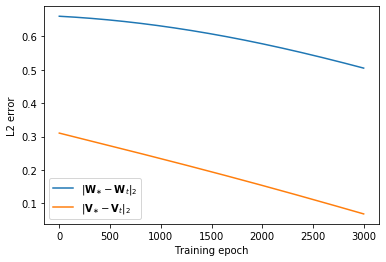
(a) ReLU

(b) Leaky ReLU (0.2)

(c) Leaky ReLU (0.05)

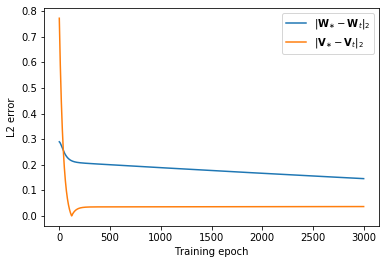
(d) Sigmoid

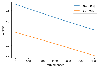
(e) Tanh

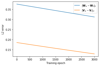
(f) Swish

The learning rate $\alpha$ is chosen as 0.1. As presented in Figure 1f, we can see clearly the stable training of the GNN and the efficiency of the algorithm. It is show that $\mathbf{W}$ converges slower than $\mathbf{v}$. Another interesting finding is that when Sigmoid is used as the activation function, the training of $\mathbf{v}$ very quickly converges to the optimum, and then lingers at the neighborhood of $\mathbf{v}_{\ast}$. This observation validates our theoretical result that the convergence is up to a statistical error. Also due to this reason, the actual convergence might be slightly slower than linear rate, which however is inevitable because of the statistical model that we consider.

GGNN Tasks

Figure 2: Training dynamics for GGNN with different activation functions.

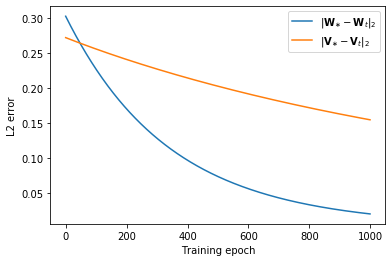
(a) ReLU

(b) Leaky ReLU (0.2)

(c) Leaky ReLU (0.05)

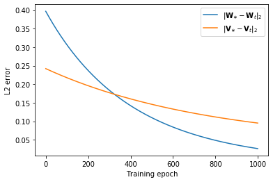
(d) Sigmoid

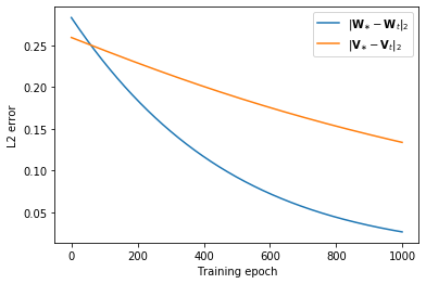
(e) Tanh

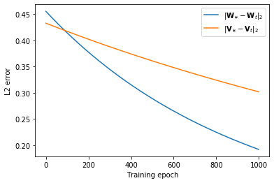
(f) Swish

For GGNN tasks, we have 1000 graphs and each graph has 5 nodes. The learning rate $\alpha$ is chosen as 0.005. As presented in Figure 2f, we can see clearly the training dynamics of the GNN and the efficiency of the algorithm. The curves are smooth, indicating that the training is very stable. By looking at the slope of the curves, for NGNN, we find that $\mathbf{W}$ converges faster than $\mathbf{v}$, which is very different from the NGNN task.

Conclusion

In this paper, we developed the first provably efficient algorithm for learning GNNs with one hidden layer for node information convolution. We investigated two types of GNNs, namely, node-level and graph-level GNNs. Our results provided a comprehensive framework and a set of tools for designing and analyzing GNNs. More importantly, our results only rely on mild condition on the activation functions, which can be satisfied by a wide range of activation functions used in practice. We constructed our training algorithm using the idea of approximate gradient descent, and proved that it recovers the true parameters of the teacher network with a linear convergence rate. How fast the algorithm converges depends on various parameters of the algorithm, which was also analytically characterized.

Broader Impact

GNN’s success has been demonstrated empirically in a wide range of applications, including social networks, recommender systems, knowledge graphs, protein interface networks, and generative models. Our work is the first to theoretically understand why GNNs work well in practice, and our algorithm converges to underlying true parameters of the teacher network linearly. Our results and tools developed in this paper provide a general framework to develop further theoretical understandings of GNNs.

There are many benefits to using the proposed algorithm, such as guaranteeing the convergence and learnability in decision-critical applications. This can help mitigate fairness, privacy and safety risks. The potential risks of increasing convergence and learnability include: (i) the risk of an undue trust in models, (ii) if the guarantee of learnability means the algorithm may now be used by those with lower levels of domain or ML expertise, this could increase the risk of the model or its outputs being used incorrectly.

Appendix A Proofs of the Main Results

General Results for NGNN and GGNN

Lemma 7.

As the assumptions in Theorem 2 hold, there exists $\eta_{W}$ such that we have

$$\|\mathbf{W}_{t+1}-\mathbf{W}_{\ast}\|_{2}-\frac{4\eta_{W}\left(1+\alpha\rho+\sqrt{1+\alpha\rho}\right)}{\rho}\leq\frac{1}{\sqrt{1+\alpha\rho}}\left[\|\mathbf{W}_{t}-\mathbf{W}_{\ast}\|_{2}-\frac{4\eta_{W}\left(1+\alpha\rho+\sqrt{1+\alpha\rho}\right)}{\rho}\right].$$ (54)

Lemma 8.

As the assumptions in Theorem 2 hold, there exist $\sigma_{m}$, $\sigma_{M}$, $L$, and $\eta_{v}$, such that we have

$$\left\lVert\mathbf{v}_{t+1}-\mathbf{v}_{\ast}\right\rVert_{2}^{2}\leq\left(1-\frac{\alpha\sigma_{m}}{2}+3\sigma^{2}_{M}\alpha^{2}\right)\left\lVert\mathbf{v}_{t}-\mathbf{v}_{\ast}\right\rVert_{2}^{2}+\left(\frac{\alpha L^{2}}{\sigma_{m}}+3L^{2}\alpha^{2}\right)\left\lVert\mathbf{W}_{t}-\mathbf{W}_{\ast}\right\rVert_{2}^{2}\left\lVert\mathbf{v}_{\ast}\right\rVert_{2}^{2}+\left(\frac{2\alpha}{\sigma_{m}}+3\alpha^{2}\right)\eta_{v}^{2}.$$ (55)

Analysis for NGNN

We first give a few definitions as follows

$$\bar{\mathbf{G}}^{W}(\mathbf{W},\mathbf{v}) =\operatorname{\mathbb{E}}\left[{\mathbf{G}}^{W}(\mathbf{W},\mathbf{v})\right]=\frac{1}{n}\left(\mathbf{W}\mathbf{v}\mathbf{v}^{\top}-\mathbf{W}^{\ast}\mathbf{v}^{\ast}\mathbf{v}^{\top}\right),$$ (56)

$$\phi(\mathbf{W},\mathbf{W}^{\prime}) =\operatorname{\mathbb{E}}_{\mathbf{H}\sim\mathcal{N}(0,1)}\left[\frac{1}{n}\left(\sigma(\mathbf{D}^{-1}\mathbf{A}\mathbf{H}\mathbf{W})\right)^{\top}\sigma(\mathbf{D}^{-1}\mathbf{A}\mathbf{H}\mathbf{W}^{\prime})\right],$$ (57)

$$\bar{\mathbf{g}}^{v}(\mathbf{W},\mathbf{v}) =\operatorname{\mathbb{E}}\left[\mathbf{g}^{v}(\mathbf{W},\mathbf{v})\right]=\left(\phi(\mathbf{W},\mathbf{W})\mathbf{v}-\phi(\mathbf{W},\mathbf{W}_{\ast})\mathbf{v}_{\ast}\right)$$ (58)

$$=\left(\phi(\mathbf{W},\mathbf{W})(\mathbf{v}-\mathbf{v}_{\ast})+\left(\phi(\mathbf{W},\mathbf{W})-\phi(\mathbf{W},\mathbf{W}_{\ast}))\right)\mathbf{v}_{\ast}\right),$$ (59)

$$\phi_{t,t} =\phi(\mathbf{W}_{t},\mathbf{W}_{t}),\phi_{t,\ast}=\phi(\mathbf{W}_{t},\mathbf{W}_{\ast}),$$ (60)

$$\bar{\mathbf{v}}_{t+1}=\mathbf{v}_{t}-\alpha\bar{\mathbf{g}}^{v}_{t}.$$ (61)

We replace the parentheses of $(\mathbf{W},\mathbf{v})$ in above definitions by subscript $t$ in proper places to denote $(\mathbf{W}_{t},\mathbf{v}_{t})$ for the ease of presentation.

Lemma 9.

If $n\geq\frac{8\ln\frac{2}{\delta}}{dd_{\min}}$, with probability at least $1-\delta$

$$\frac{\left\lVert\mathbf{G}^{W}(\mathbf{W},\mathbf{v})-\mathbf{G}^{W}(\mathbf{W}^{\prime},\mathbf{v})\right\rVert_{2}}{\left\lVert\mathbf{W}-\mathbf{W}^{\prime}\right\rVert_{2}}\leq D_{0}^{2}\left\lVert\Xi^{-1}\right\rVert_{2}(d+4d\bar{d}),$$ (62)

$$\frac{\left\lVert\mathbf{G}^{W}(\mathbf{W},\mathbf{v})-\mathbf{G}^{W}(\mathbf{W},\mathbf{v}^{\prime})\right\rVert_{2}}{\left\lVert\mathbf{v}-\mathbf{v}^{\prime}\right\rVert_{2}}\leq 4D_{0}\left\lVert\Xi^{-1}\right\rVert_{2}(d+4d\bar{d})L_{\sigma},$$ (63)

$$\frac{\left\lVert\mathbf{g}^{v}(\mathbf{W},\mathbf{v})-\mathbf{g}^{v}(\mathbf{W}^{\prime},\mathbf{v})\right\rVert_{2}}{\left\lVert\mathbf{W}-\mathbf{W}^{\prime}\right\rVert_{2}}\leq 5(d+4d\bar{d})D_{0}L_{\sigma}+\frac{d+4d\bar{d}}{2}+\nu^{2},$$ (64)

$$\frac{\left\lVert\mathbf{g}^{v}(\mathbf{W},\mathbf{v})-\mathbf{g}^{v}(\mathbf{W},\mathbf{v}^{\prime})\right\rVert_{2}}{\left\lVert\mathbf{v}-\mathbf{v}^{\prime}\right\rVert_{2}}\leq{L_{\sigma}^{2}}(d+4d\bar{d}).$$ (65)

Lemma 10.

If $\sqrt{n\log n}\geq\frac{3}{2}\log\frac{2}{\delta}$, with probability at least $1-\delta$

$$\left\lVert\mathbf{G}^{W}-\bar{\mathbf{G}}^{W}\right\rVert_{2}\leq\frac{4}{c}\sqrt{{\frac{\log n}{n}}}\left\lVert\Xi^{-1}\right\rVert_{2}D_{0}\left(D_{0}\frac{d}{d_{\min}}(1+|\sigma(0)|)+\sqrt{\frac{d}{d_{\min}}}\nu\right),$$ (66)

$$\left\lVert\mathbf{g}^{v}-\bar{\mathbf{g}}^{v}\right\rVert_{2}\leq\frac{2}{c}\sqrt{{\frac{\log n}{n}}}\left(D_{0}\frac{d}{d_{\min}}(1+|\sigma(0)|)^{2}+\sqrt{\frac{d}{d_{\min}}}(1+|\sigma(0)|)\nu\right),$$ (67)

for some absolute constant $c$.

Analysis for GGNN

We first give a few definitions as follows

$$\bar{\mathbf{G}}^{W}(\mathbf{W},\mathbf{v}) =\operatorname{\mathbb{E}}\left[{\mathbf{G}}^{W}(\mathbf{W},\mathbf{v})\right]=\mathbf{W}\mathbf{v}\mathbf{v}^{\top}-\mathbf{W}^{\ast}\mathbf{v}^{\ast}\mathbf{v}^{\top},$$ (68)

$$\phi_{j}(\mathbf{W},\mathbf{W}^{\prime}) =\operatorname{\mathbb{E}}_{\mathbf{H}_{j}\sim\mathcal{N}(0,1)}\left[\left(\mathbf{a}_{j}\sigma(\mathbf{D}_{j}^{-1}\mathbf{A}_{j}\mathbf{H}_{j}\mathbf{W})\right)^{\top}\mathbf{a}_{j}\sigma(\mathbf{D}_{j}^{-1}\mathbf{A}_{j}\mathbf{H}_{j}\mathbf{W}^{\prime})\right],$$ (69)

$$\phi(\mathbf{W},\mathbf{W}^{\prime}) =\frac{1}{n}\sum_{j=1}^{n}\phi_{j}(\mathbf{W},\mathbf{W}^{\prime}),$$ (70)

$$\bar{\mathbf{g}}^{v}(\mathbf{W},\mathbf{v}) =\operatorname{\mathbb{E}}\left[\mathbf{g}^{v}(\mathbf{W},\mathbf{v})\right]=\frac{1}{n}\sum_{j=1}^{n}\phi_{j}(\mathbf{W},\mathbf{W})\mathbf{v}-\frac{1}{n}\sum_{j=1}^{n}\phi_{j}(\mathbf{W},\mathbf{W}_{\ast})\mathbf{v}_{\ast}$$ (71)

$$=\phi(\mathbf{W},\mathbf{W})\mathbf{v}-\phi(\mathbf{W},\mathbf{W}_{\ast})\mathbf{v}_{\ast}$$ (72)

$$=\phi(\mathbf{W},\mathbf{W})(\mathbf{v}-\mathbf{v}_{\ast})+\left(\phi(\mathbf{W},\mathbf{W})-\phi(\mathbf{W},\mathbf{W}_{\ast})\right)\mathbf{v}_{\ast},$$ (73)

$$\phi_{t,t} =\phi(\mathbf{W}_{t},\mathbf{W}_{t}),\phi_{t,\ast}=\phi(\mathbf{W}_{t},\mathbf{W}_{\ast}).$$ (74)

We replace the parentheses of $(\mathbf{W},\mathbf{v})$ by subscript $t$ in proper places to denote $(\mathbf{W}_{t},\mathbf{v}_{t})$ for the ease of presentation.

Lemma 11.

If $\sum_{j=1}^{n}n_{j}\geq\frac{8\ln\frac{1}{\delta}}{d}$, with probability at least $1-\delta$

$$\frac{\left\lVert\mathbf{G}^{W}(\mathbf{W},\mathbf{v})-\mathbf{G}^{W}(\mathbf{W}^{\prime},\mathbf{v})\right\rVert_{2}}{\left\lVert\mathbf{W}-\mathbf{W}^{\prime}\right\rVert_{2}}\leq 2dD_{0}^{2}\left\lVert\Xi^{-1}\right\rVert_{2}n^{2}_{\max},$$ (75)

$$\frac{\left\lVert\mathbf{G}^{W}(\mathbf{W},\mathbf{v})-\mathbf{G}^{W}(\mathbf{W},\mathbf{v}^{\prime})\right\rVert_{2}}{\left\lVert\mathbf{v}-\mathbf{v}^{\prime}\right\rVert_{2}}\leq 8D_{0}d\Xi^{-1}n^{2}_{\max}L_{\sigma},$$ (76)

$$\frac{\left\lVert\mathbf{g}^{v}(\mathbf{W},\mathbf{v})-\mathbf{g}^{v}(\mathbf{W}^{\prime},\mathbf{v})\right\rVert_{2}}{\left\lVert\mathbf{W}-\mathbf{W}^{\prime}\right\rVert_{2}}\leq 10dD_{0}L_{\sigma}n_{\max}^{2}+{d\sqrt{n^{3}_{\max}}}+{\sqrt{n_{\max}}}\nu^{2},$$ (77)

$$\frac{\left\lVert\mathbf{g}^{v}(\mathbf{W},\mathbf{v})-\mathbf{g}^{v}(\mathbf{W},\mathbf{v}^{\prime})\right\rVert_{2}}{\left\lVert\mathbf{v}-\mathbf{v}^{\prime}\right\rVert_{2}}\leq 2d{L_{\sigma}^{2}}n_{\max}^{2}.$$ (78)

Lemma 12.

If $\sqrt{n\log n}\geq\frac{3}{2}\log\frac{2}{\delta}$, with probability at least $1-\delta$

$$\left\lVert\mathbf{G}^{W}-\bar{\mathbf{G}}^{W}\right\rVert_{2}\leq\frac{4}{c}\sqrt{\frac{\log n}{n}}\left\lVert\Xi^{-1}\right\rVert_{2}\sqrt{n_{\max}}\left(\sqrt{n_{\max}}2(1+|\sigma(0)|)D_{0}+\nu\right),$$ (79)

$$\left\lVert\mathbf{g}^{v}-\bar{\mathbf{g}}^{v}\right\rVert_{2}\leq\frac{2}{c}\sqrt{\frac{\log n}{n}}\sqrt{n_{\max}}2(1+|\sigma(0)|)\left(\sqrt{n_{\max}}2(1+|\sigma(0)|)D_{0}+\nu\right),$$ (80)

for some absolute constant $c$.

Useful Lemmas and Results

Lemma 13.

If $n\geq\frac{8\ln\frac{1}{\delta}}{dd_{\min}}$ with $d_{\min}$ being the smallest node degree in the graph, then with probability at least $1-\delta$ for NGNN

$$\frac{1}{n}\left\lVert\mathbf{D}^{-1}\mathbf{A}\mathbf{H}\right\rVert_{2}^{2}\leq d+4d\bar{d},$$ (81)

where $\bar{d}=\frac{\sum_{i=1}^{n}\frac{1}{d_{i}}}{n}$.

Lemma 14.

If $\sum_{j=1}^{n}n_{j}\geq\frac{8\ln\frac{1}{\delta}}{d}$, with probability at least $1-\delta$ for GGNN

$$\frac{1}{n}\sum_{j=1}^{n}\left\lVert\mathbf{H}_{j}^{\top}\mathbf{A}_{j}^{\top}(\mathbf{D}_{j}^{-1})^{\top}\right\rVert_{2}\left\lVert\mathbf{a}_{j}\right\rVert_{2}^{2}\left\lVert\mathbf{D}_{j}^{-1}\mathbf{A}_{j}\mathbf{H}_{j}\right\rVert_{2}\leq 2dn^{2}_{\max}.$$ (82)

We provide several concentration results for random variables, and we do not provide corresponding proofs as the results are commonly acknowledged.

Lemma 15 (Hoeffding Inequality for Chi-square Distribution).

$z_{k}\sim\mathcal{N}(0,1)$, for all $t\in[0,1]$ then the probability

$$P\left(\sum_{k=1}^{n}z_{k}^{2}\leq(t+1)n\right)\geq 1-\exp(-\frac{nt^{2}}{8}).$$ (83)

Lemma 16.

Let $X_{1},\ldots,X_{n}$ be independent sub-exponential random variables such that $\mathcal{E}X_{i}=\mu_{i}$ and $X_{i}\in SE(\nu_{i}^{2},\alpha_{i})$. Then

$$\sum_{i=1}^{n}(X_{i}-\mu_{i})\in SE(\sum_{i=1}^{n}\nu_{i}^{2},\max_{i}\alpha_{i}).$$ (84)

In particular, denote $\nu_{\ast}^{2}=\sum_{i=1}^{n}\nu_{i}^{2},\alpha_{\ast}=\max_{i}\alpha_{i}$. Then,

$$P\left(\frac{1}{n}\sum_{i=1}^{n}(X_{i}-\mu_{i})\geq t\right)\leq\begin{cases}\exp\left(-\frac{nt^{2}}{2\nu_{\ast}^{2}}\right),&\text{if}\ 0<nt<\frac{\nu_{\ast}^{2}}{\alpha_{\ast}}\\ \exp\left(-\frac{nt}{2\alpha_{\ast}}\right),&\text{otherwise}\end{cases}.$$ (85)

Lemma 17 ((Honorio and Jaakkola 2014)).

Let $s$ be a sub-Gaussian variable with parameter $\sigma_{s}$ and mean $\mu_{s}=\mathbb{E}s$. Then, $s^{2}\in SE(4\sigma_{s}^{2},4\sigma_{s}^{2})$.

Lemma 18.

A random variable $x$ is called sub-Gaussian, if

$$P(|x|\geq t)\leq 2e^{-ct^{2}},$$ (86)

for some $c>0$ and $\|x\|_{\psi_{2}}\leq c$. Then let $x_{1},\ldots,x_{n}$ be zero-mean independent sub-Gaussian random variables, the general version of the Hoeffding’s inequality states that

$$P\left(|\sum_{i=1}^{n}x_{i}|\geq t\right)\leq 2\exp\left(-\frac{ct^{2}}{\sum_{i=1}^{n}\|x_{i}\|^{2}_{\psi_{2}}}\right).$$ (87)

Result 1.

For node-level GNN tasks, based on Lemma 13, the largest eigenvalue of $\phi_{t,t}$ can be well bounded such that $\sigma_{M}\leq(d+4d\bar{d})L_{\sigma}^{2}$. Similarly, we have $L\leq(d+4d\bar{d})L_{\sigma}$. By Theorem 2.2 in (Yaskov 2014), almost surely, the smallest eigenvalues of $\phi_{t,t}$ and $\phi_{t,\ast}$ are lower bounded by an absolute constant, which we denote here by $\sigma_{m}\leq L_{\sigma}^{2}d_{out}$ and $\sigma^{\prime}_{m}\leq L_{\sigma}^{2}d_{out}$, respectively .

For graph-level GNN tasks, based on Lemma 14, the largest eigenvalue of $\phi_{t,t}$ can be well bounded such that $\sigma_{M}\leq 2dL_{\sigma}^{2}n_{\max}^{2}$. Similarly, we have $L\leq 2dn^{2}_{\max}L_{\sigma}$. By Theorem 2.2 in (Yaskov 2014), almost surely, the smallest eigenvalues of $\phi_{t,t}$ and $\phi_{t,\ast}$ are lower bounded by an absolute constant, which we denote here by $\sigma_{m}\leq L_{\sigma}^{2}d_{out}$ and $\sigma^{\prime}_{m}\leq L_{\sigma}^{2}d_{out}$, respectively.

We will use the above equality in the paper, and the results derived still hold.

Proofs of Lemmas and Theorems

In this section, we provide proofs of the above lemmas and the main theorems.

Proof of Lemma 7

Proof.

Define

$$\bar{\mathbf{U}}_{t+1}=\mathbf{W}_{t}-\alpha\bar{\mathbf{G}}^{W}_{t}=\mathbf{W}_{t}(\mathbf{I}-\alpha\mathbf{v}_{t}\mathbf{v}_{t}^{\top})+\alpha\mathbf{W}^{\ast}\mathbf{v}^{\ast}\mathbf{v}_{t}^{\top},$$ (88)

and

$$\hat{\mathbf{U}}=\bar{\mathbf{U}}_{t+1}/\|\bar{\mathbf{U}}_{t+1}\|_{2}.$$ (89)

If $\mathbf{I}-\alpha\mathbf{v}_{t}\mathbf{v}_{t}^{\top}\geq 0$ and $\mathbf{v}_{t}^{\top}\mathbf{v}^{\ast}\geq\rho$, $\hat{\mathbf{U}}$ is closer to $\mathbf{W}^{\ast}$ than $\mathbf{U}^{\prime}$, i.e., $\|\hat{\mathbf{U}}-\mathbf{W}^{\ast}\|_{2}\leq\|{\mathbf{U}^{\prime}}-\mathbf{W}^{\ast}\|_{2}$ where $\mathbf{U}^{\prime}=\frac{\mathbf{W}_{t}+\alpha\rho\mathbf{W}^{\ast}}{\|\mathbf{W}_{t}+\alpha\rho\mathbf{W}^{\ast}\|_{2}}$. Therefore,

$$1-\frac{1}{2}\operatorname{Tr}\left(\left(\mathbf{W}_{\ast}-\hat{\mathbf{U}}\right)^{\top}\left(\mathbf{W}_{\ast}-\hat{\mathbf{U}}\right)\right)\geq 1-\frac{1}{2}\operatorname{Tr}\left(\left(\mathbf{W}_{\ast}-{\mathbf{U}}^{\prime}\right)^{\top}\left(\mathbf{W}_{\ast}-{\mathbf{U}}^{\prime}\right)\right).$$ (90)

Thus, we have

$$\operatorname{Tr}\left(\frac{1}{2}\mathbf{W}^{\top}_{\ast}\mathbf{W}_{\ast}+\frac{1}{2}\hat{\mathbf{U}}^{\top}\hat{\mathbf{U}}-\frac{1}{2}\left(\mathbf{W}_{\ast}-\hat{\mathbf{U}}\right)^{\top}\left(\mathbf{W}_{\ast}-\hat{\mathbf{U}}\right)\right)$$ (91)

$$\geq\operatorname{Tr}\left(\frac{1}{2}\mathbf{W}^{\top}_{\ast}\mathbf{W}_{\ast}+\frac{1}{2}{\mathbf{U}^{\prime}}^{\top}{\mathbf{U}}^{\prime}-\frac{1}{2}\left(\mathbf{W}_{\ast}-{\mathbf{U}}^{\prime}\right)^{\top}\left(\mathbf{W}_{\ast}-{\mathbf{U}}^{\prime}\right)\right),$$ (92)

which leads to

$$\operatorname{Tr}\left(\frac{1}{2}\mathbf{W}^{\top}_{\ast}\mathbf{W}_{\ast}+\frac{1}{2}\hat{\mathbf{U}}^{\top}\hat{\mathbf{U}}-\frac{1}{2}\left(\mathbf{W}_{\ast}-\hat{\mathbf{U}}\right)^{\top}\left(\mathbf{W}_{\ast}-\hat{\mathbf{U}}\right)\right)$$ (93)

$$\geq\operatorname{Tr}\left(\mathbf{W}^{\top}_{\ast}{\mathbf{U}}^{\prime}\right)=\operatorname{Tr}\left(\mathbf{W}^{\top}_{\ast}\frac{\mathbf{W}_{t}+\alpha\rho\mathbf{W}^{\ast}}{\|\mathbf{W}_{t}+\alpha\rho\mathbf{W}^{\ast}\|_{2}}\right)$$ (94)

$$\geq\operatorname{Tr}\left(\mathbf{W}^{\top}_{\ast}\frac{\mathbf{W}_{t}+\alpha\rho\mathbf{W}^{\ast}}{1+\alpha\rho}\right)$$ (95)

$$=\operatorname{Tr}\left(\frac{\alpha\rho\mathbf{W}^{\top}_{\ast}\mathbf{W}^{\ast}}{1+\alpha\rho}+\frac{1}{1+\alpha\rho}\left(\frac{1}{2}\mathbf{W}^{\top}_{\ast}\mathbf{W}_{\ast}+\frac{1}{2}{\mathbf{W}_{t}}^{\top}\mathbf{W}_{t}-\frac{1}{2}\left(\mathbf{W}_{\ast}-\mathbf{W}_{t}\right)^{\top}\left(\mathbf{W}_{\ast}-\mathbf{W}_{t}\right)\right)\right).$$ (96)

Hence, we have

$$\operatorname{Tr}\left(\frac{1}{2}\mathbf{W}^{\top}_{\ast}\mathbf{W}_{\ast}+\frac{1}{2}\hat{\mathbf{U}}^{\top}\hat{\mathbf{U}}-\frac{1}{2}\left(\mathbf{W}_{\ast}-\hat{\mathbf{U}}\right)^{\top}\left(\mathbf{W}_{\ast}-\hat{\mathbf{U}}\right)\right)$$ (97)

$$\geq\operatorname{Tr}\left(\frac{\alpha\rho\mathbf{W}^{\top}_{\ast}\mathbf{W}^{\ast}}{1+\alpha\rho}+\frac{1}{1+\alpha\rho}\left(\frac{1}{2}\mathbf{W}^{\top}_{\ast}\mathbf{W}_{\ast}+\frac{1}{2}{\mathbf{W}_{t}}^{\top}\mathbf{W}_{t}-\frac{1}{2}\left(\mathbf{W}_{\ast}-\mathbf{W}_{t}\right)^{\top}\left(\mathbf{W}_{\ast}-\mathbf{W}_{t}\right)\right)\right).$$ (98)

Rearranging the terms yields

$$\operatorname{Tr}\left(\left(\mathbf{W}_{\ast}-\hat{\mathbf{U}}\right)^{\top}\left(\mathbf{W}_{\ast}-\hat{\mathbf{U}}\right)\right)$$ (99)

$$\leq\operatorname{Tr}\left(\mathbf{W}^{\top}_{\ast}\mathbf{W}_{\ast}+\hat{\mathbf{U}}^{\top}\hat{\mathbf{U}}-\frac{1+2\alpha\rho}{1+\alpha\rho}\mathbf{W}^{\top}_{\ast}\mathbf{W}_{\ast}-\frac{1}{1+\alpha\rho}{\mathbf{W}_{t}}^{\top}\mathbf{W}_{t}+\frac{1}{1+\alpha\rho}\left(\mathbf{W}_{\ast}-\mathbf{W}_{t}\right)^{\top}\left(\mathbf{W}_{\ast}-\mathbf{W}_{t}\right)\right),$$ (100)

which is equivalent to

$$\|\mathbf{W}_{\ast}-\hat{\mathbf{U}}\|_{2}^{2}\leq 1+1-\frac{1+2\alpha\rho}{1+\alpha\rho}-\frac{1}{1+\alpha\rho}+\frac{1}{1+\alpha\rho}\|\mathbf{W}_{\ast}-\mathbf{W}_{t}\|_{2}^{2}=\frac{1}{1+\alpha\rho}\|\mathbf{W}_{\ast}-\mathbf{W}_{t}\|_{2}^{2}.$$ (101)

Therefore, we obtain

$$\|\mathbf{W}_{\ast}-\hat{\mathbf{U}}\|_{2}\leq\frac{\|\mathbf{W}_{\ast}-\mathbf{W}_{t}\|_{2}}{\sqrt{1+\alpha\rho}}.$$ (102)

As we have in Lemmas 10 and 12 that

$$\|\mathbf{U}_{t+1}-\bar{\mathbf{U}}_{t+1}\|_{2}=\alpha\left\lVert\mathbf{G}^{W}_{t}-\bar{\mathbf{G}}_{t}^{W}\right\rVert_{2}\leq\alpha\eta_{W},$$ (103)

it results in

$$\|\mathbf{W}_{t+1}-\hat{\mathbf{U}}\|_{2}\leq\frac{2\alpha\eta_{W}}{\|\bar{\mathbf{U}}_{t+1}\|_{2}}.$$ (104)

By Theorem 3, we have $\operatorname{Tr}(\mathbf{W}^{\top}_{\ast}\mathbf{W}_{t})\geq\mathbf{0}$. Hence,

$$\|\bar{\mathbf{U}}_{t+1}\|_{2}=\|\mathbf{W}_{t}(\mathbf{I}-\alpha\mathbf{v}_{t}\mathbf{v}_{t}^{\top})+\alpha\mathbf{W}^{\ast}\mathbf{v}^{\ast}\mathbf{v}_{t}^{\top}\|_{2}\geq 1-\alpha\|\mathbf{v}_{t}\|^{2}_{2}\geq 1-\alpha D_{0}^{2}\geq\frac{1}{2}.$$ (105)

Thus, it yields

$$\|\mathbf{W}_{t+1}-\hat{\mathbf{U}}\|_{2}\leq{4\alpha\eta_{W}}.$$ (106)

By triangle inequality,

$$\|\mathbf{W}_{t+1}-\mathbf{W}_{\ast}\|_{2}\leq\|\mathbf{W}_{\ast}-\hat{\mathbf{U}}\|_{2}+\|\mathbf{W}_{t+1}-\hat{\mathbf{U}}\|_{2}\leq{4\alpha\eta_{W}}+\frac{\|\mathbf{W}_{\ast}-\mathbf{W}_{t}\|_{2}}{\sqrt{1+\alpha\rho}},$$ (107)

which results in

$$\|\mathbf{W}_{t+1}-\mathbf{W}_{\ast}\|_{2}-\frac{4\eta_{W}\left(1+\alpha\rho+\sqrt{1+\alpha\rho}\right)}{\rho}\leq\frac{1}{\sqrt{1+\alpha\rho}}\left[\|\mathbf{W}_{t}-\mathbf{W}_{\ast}\|_{2}-\frac{4\eta_{W}\left(1+\alpha\rho+\sqrt{1+\alpha\rho}\right)}{\rho}\right].$$ (108)

∎

Proof of Lemma 8

Proof.

First ,we define

$$\bar{\mathbf{v}}_{t+1}=\mathbf{v}_{t}-\alpha\bar{\mathbf{g}}^{v}_{t}.$$ (109)

Then, it directly follows

$$\left\lVert\bar{\mathbf{v}}_{t+1}-\mathbf{v}_{\ast}\right\rVert_{2}=\left\lVert\left(\mathbf{I}-\alpha\phi_{t,t}\right)\left(\mathbf{v}_{t}-\mathbf{v}_{\ast}\right)-\alpha\left(\phi_{t,t}-\phi_{t,\ast}\right)\mathbf{v}_{\ast}\right\rVert_{2}.$$ (110)

As we have in Lemmas 10 and 12 that

$$\left\lVert\mathbf{v}_{t+1}-\bar{\mathbf{v}}_{t+1}\right\rVert_{2}=\alpha\left\lVert\mathbf{g}_{t}^{v}-\bar{\mathbf{g}}_{t}^{v}\right\rVert_{2}\leq\alpha\eta_{v}.$$ (111)

By triangle inequality, we have

$$\left\lVert\mathbf{v}_{t+1}-\mathbf{v}_{\ast}\right\rVert_{2}\leq\left\lVert\mathbf{I}-\alpha\phi_{t,t}\right\rVert_{2}\left\lVert\mathbf{v}_{t}-\mathbf{v}_{\ast}\right\rVert_{2}+\alpha\left\lVert\phi_{t,t}-\phi_{t,\ast}\right\rVert_{2}\left\lVert\mathbf{v}_{\ast}\right\rVert_{2}+\alpha\eta_{v}$$ (112)

According to Lemma 10 and Lemma 12, it can be written as

$$\left\lVert\phi_{t,t}-\phi_{t,\ast}\right\rVert_{2}\leq L\left\lVert\mathbf{W}-\mathbf{W}_{\ast}\right\rVert_{2},$$ (113)

where $L$ is given in Result 1. Thus, we can write

$$\left\lVert\mathbf{v}_{t+1}-\mathbf{v}_{\ast}\right\rVert_{2}\leq\left\lVert\mathbf{I}-\alpha\phi_{t,t}\right\rVert_{2}\left\lVert\mathbf{v}_{t}-\mathbf{v}_{\ast}\right\rVert_{2}+\alpha L\left\lVert\mathbf{W}-\mathbf{W}_{\ast}\right\rVert_{2}\left\lVert\mathbf{v}_{\ast}\right\rVert_{2}+\alpha\eta_{v}.$$ (114)

Additionally, we also have

$$(\mathbf{v}_{t}-\mathbf{v}_{\ast})^{\top}\mathbf{g}_{t}^{v} \geq(\mathbf{v}_{t}-\mathbf{v}_{\ast})^{\top}\bar{\mathbf{g}}_{t}^{v}-\eta_{v}\left\lVert\mathbf{v}_{t}-\mathbf{v}_{\ast}\right\rVert_{2}$$ (115)

$$=(\mathbf{v}_{t}-\mathbf{v}_{\ast})^{\top}\phi_{t,t}(\mathbf{v}_{t}-\mathbf{v}_{\ast})+(\mathbf{v}_{t}-\mathbf{v}_{\ast})^{\top}\left(\phi_{t,t}-\phi_{t,\ast}\right)\mathbf{v}_{\ast}-\eta_{v}\left\lVert\mathbf{v}_{t}-\mathbf{v}_{\ast}\right\rVert_{2}$$ (116)

$$\geq\sigma_{m}\left\lVert\mathbf{v}_{t}-\mathbf{v}_{\ast}\right\rVert_{2}^{2}-L\left\lVert\mathbf{W}_{t}-\mathbf{W}_{\ast}\right\rVert_{2}\left\lVert\mathbf{v}_{t}-\mathbf{v}_{\ast}\right\rVert_{2}\left\lVert\mathbf{v}_{\ast}\right\rVert_{2}-\eta_{v}\left\lVert\mathbf{v}_{t}-\mathbf{v}_{\ast}\right\rVert_{2}$$ (117)

$$\geq\sigma_{m}\left\lVert\mathbf{v}_{t}-\mathbf{v}_{\ast}\right\rVert_{2}^{2}-\frac{1}{2}\left(\frac{L^{2}}{\sigma_{m}}\left\lVert\mathbf{W}_{t}-\mathbf{W}_{\ast}\right\rVert_{2}^{2}\left\lVert\mathbf{v}_{\ast}\right\rVert_{2}^{2}+\sigma_{m}\left\lVert\mathbf{v}_{t}-\mathbf{v}_{\ast}\right\rVert_{2}^{2}\right)-\eta_{v}\left\lVert\mathbf{v}_{t}-\mathbf{v}_{\ast}\right\rVert_{2}$$ (118)

$$\geq\frac{\sigma_{m}}{2}\left\lVert\mathbf{v}_{t}-\mathbf{v}_{\ast}\right\rVert_{2}^{2}-\frac{L^{2}}{2\sigma_{m}}\left\lVert\mathbf{W}_{t}-\mathbf{W}_{\ast}\right\rVert_{2}^{2}\left\lVert\mathbf{v}_{\ast}\right\rVert_{2}^{2}-\frac{1}{2}\left(\frac{\sigma_{m}}{2}\left\lVert\mathbf{v}_{t}-\mathbf{v}_{\ast}\right\rVert_{2}^{2}+\frac{2}{\sigma_{m}}\eta_{v}^{2}\right)$$ (119)

$$=\frac{\sigma_{m}}{4}\left\lVert\mathbf{v}_{t}-\mathbf{v}_{\ast}\right\rVert_{2}^{2}-\frac{L^{2}}{2\sigma_{m}}\left\lVert\mathbf{W}_{t}-\mathbf{W}_{\ast}\right\rVert_{2}^{2}\left\lVert\mathbf{v}_{\ast}\right\rVert_{2}^{2}-\frac{1}{\sigma_{m}}\eta_{v}^{2}.$$ (120)

The second inequality is due to the definition that $\sigma_{m}$ is the smallest non-negative eigenvalue of the matrix $\phi_{t,t}$ and (113). Therefore, we have

$$\left\lVert\mathbf{v}_{t+1}-\mathbf{v}_{\ast}\right\rVert_{2}^{2}=\left\lVert\mathbf{v}_{t}-\alpha\mathbf{g}_{t}^{v}-\mathbf{v}_{\ast}\right\rVert_{2}^{2}=\left\lVert\mathbf{v}_{t}-\mathbf{v}_{\ast}\right\rVert_{2}^{2}-2\alpha(\mathbf{v}_{t}-\mathbf{v}_{\ast})^{\top}\mathbf{g}_{t}^{v}+\alpha^{2}\left\lVert\mathbf{g}_{t}^{v}\right\rVert_{2}^{2}$$

$$\leq\left\lVert\mathbf{v}_{t}-\mathbf{v}_{\ast}\right\rVert_{2}^{2}-\frac{\alpha\sigma_{m}}{2}\left\lVert\mathbf{v}_{t}-\mathbf{v}_{\ast}\right\rVert_{2}^{2}+\frac{\alpha L^{2}}{\sigma_{m}}\left\lVert\mathbf{W}_{t}-\mathbf{W}_{\ast}\right\rVert_{2}^{2}\left\lVert\mathbf{v}_{\ast}\right\rVert_{2}^{2}+\frac{2\alpha}{\sigma_{m}}\eta_{v}^{2}+\alpha^{2}\left\lVert\mathbf{g}_{t}^{v}\right\rVert_{2}^{2}.$$ (121)

Now, we can write

$$\left\lVert\mathbf{g}_{t}^{v}\right\rVert_{2} \leq\left\lVert\bar{\mathbf{g}}_{t}^{v}\right\rVert_{2}+\eta_{v}\leq\left\lVert\phi_{t,t}(\mathbf{v}_{t}-\mathbf{v}_{\ast})+\left(\phi_{t,t}-\phi_{t,\ast}\right)\mathbf{v}_{\ast}\right\rVert_{2}+\eta_{v}$$ (122)

$$\leq\left\lVert\phi_{t,t}(\mathbf{v}_{t}-\mathbf{v}_{\ast})\right\rVert_{2}+\left\lVert\left(\phi_{t,t}-\phi_{t,\ast}\right)\mathbf{v}_{\ast}\right\rVert_{2}+\eta_{v}$$ (123)

$$\leq\sigma_{M}\left\lVert\mathbf{v}_{t}-\mathbf{v}_{\ast}\right\rVert_{2}+L\left\lVert\mathbf{W}_{t}-\mathbf{W}_{\ast}\right\rVert_{2}\left\lVert\mathbf{v}_{\ast}\right\rVert_{2}+\eta_{v},$$ (124)

where $\sigma_{M}$ is the largest non-negative eigenvalue of the matrix $\phi_{t,t}$. Hence, it results in

$$\left\lVert\mathbf{g}_{t}^{v}\right\rVert_{2}^{2}\leq 3\sigma^{2}_{M}\left\lVert\mathbf{v}_{t}-\mathbf{v}_{\ast}\right\rVert_{2}^{2}+3L^{2}\left\lVert\mathbf{W}_{t}-\mathbf{W}_{\ast}\right\rVert_{2}^{2}\left\lVert\mathbf{v}_{\ast}\right\rVert_{2}^{2}+3\eta_{v}^{2}.$$ (125)

Plugging into the inequality (A) provides

$$\left\lVert\mathbf{v}_{t+1}-\mathbf{v}_{\ast}\right\rVert_{2}^{2}\leq\left(1-\frac{\alpha\sigma_{m}}{2}+3\sigma^{2}_{M}\alpha^{2}\right)\left\lVert\mathbf{v}_{t}-\mathbf{v}_{\ast}\right\rVert_{2}^{2}+\left(\frac{\alpha L^{2}}{\sigma_{m}}+3L^{2}\alpha^{2}\right)\left\lVert\mathbf{W}_{t}-\mathbf{W}_{\ast}\right\rVert_{2}^{2}\left\lVert\mathbf{v}_{\ast}\right\rVert_{2}^{2}+\left(\frac{2\alpha}{\sigma_{m}}+3\alpha^{2}\right)\eta_{v}^{2}.$$ (126)

∎

Proof of Lemma 9

First, we can write

$$\left\lVert\mathbf{G}^{W}(\mathbf{W},\mathbf{v})-\mathbf{G}^{W}(\mathbf{W}^{\prime},\mathbf{v})\right\rVert_{2}=\left\lVert\frac{1}{n}\Xi^{-1}\mathbf{H}^{\top}\mathbf{A}^{\top}(\mathbf{D}^{-1})^{\top}\left(\sigma(\mathbf{D}^{-1}\mathbf{A}\mathbf{H}\mathbf{W})-\sigma(\mathbf{D}^{-1}\mathbf{A}\mathbf{H}\mathbf{W}^{\prime})\right)\mathbf{v}\mathbf{v}^{\top}\right\rVert_{2}$$ (127)

$$\leq\frac{1}{n}\left\lVert\Xi^{-1}\right\rVert_{2}\left\lVert\mathbf{H}^{\top}\mathbf{A}^{\top}(\mathbf{D}^{-1})^{\top}\right\rVert_{2}\left\lVert\sigma(\mathbf{D}^{-1}\mathbf{A}\mathbf{H}\mathbf{W})-\sigma(\mathbf{D}^{-1}\mathbf{A}\mathbf{H}\mathbf{W}^{\prime})\right\rVert_{2}\left\lVert\mathbf{v}\right\rVert_{2}^{2}$$ (128)

$$\leq\frac{1}{n}\left\lVert\Xi^{-1}\right\rVert_{2}\left\lVert\mathbf{H}^{\top}\mathbf{A}^{\top}(\mathbf{D}^{-1})^{\top}\right\rVert_{2}\left\lVert\mathbf{D}^{-1}\mathbf{A}\mathbf{H}\mathbf{W}-\mathbf{D}^{-1}\mathbf{A}\mathbf{H}\mathbf{W}^{\prime}\right\rVert_{2}\left\lVert\mathbf{v}\right\rVert_{2}^{2}.$$ (129)

Then, using the result from Lemma 13 with probability at least $1-\delta$ if $n\geq\frac{8\ln\frac{1}{\delta}}{dd_{\min}}$

$$\left\lVert\mathbf{G}^{W}(\mathbf{W},\mathbf{v})-\mathbf{G}^{W}(\mathbf{W}^{\prime},\mathbf{v})\right\rVert_{2} \leq D_{0}^{2}\left\lVert\Xi^{-1}\right\rVert_{2}\frac{1}{n}\left\lVert\mathbf{D}^{-1}\mathbf{A}\mathbf{H}\right\rVert_{2}^{2}\left\lVert\mathbf{W}-\mathbf{W}^{\prime}\right\rVert_{2}$$ (130)

$$\leq D_{0}^{2}\left\lVert\Xi^{-1}\right\rVert_{2}\left\lVert\mathbf{W}-\mathbf{W}^{\prime}\right\rVert_{2}(d+4d\bar{d}).$$ (131)

Thus, we have the desired result as

$$\frac{\left\lVert\mathbf{G}^{W}(\mathbf{W},\mathbf{v})-\mathbf{G}^{W}(\mathbf{W}^{\prime},\mathbf{v})\right\rVert_{2}}{\left\lVert\mathbf{W}-\mathbf{W}^{\prime}\right\rVert_{2}}\leq D_{0}^{2}\left\lVert\Xi^{-1}\right\rVert_{2}(d+4d\bar{d}).$$ (132)

Next, we can have with probability at least $1-\delta$ if $n\geq\frac{8\ln\frac{1}{\delta}}{dd_{\min}}$

$$\left\lVert\mathbf{G}^{W}(\mathbf{W},\mathbf{v})-\mathbf{G}^{W}(\mathbf{W},\mathbf{v}^{\prime})\right\rVert_{2}=\left\lVert\frac{1}{n}\Xi^{-1}\mathbf{H}^{\top}\mathbf{A}^{\top}(\mathbf{D}^{-1})^{\top}\sigma(\mathbf{D}^{-1}\mathbf{A}\mathbf{H}\mathbf{W})\left(\mathbf{v}\mathbf{v}^{\top}-\mathbf{v}^{\prime}\mathbf{v}^{\prime\top}\right)\right\rVert_{2}$$ (133)

$$\leq L_{\sigma}\frac{1}{n}\left\lVert\Xi^{-1}\right\rVert_{2}\left\lVert\mathbf{H}^{\top}\mathbf{A}^{\top}(\mathbf{D}^{-1})^{\top}\right\rVert_{2}\left\lVert\mathbf{D}^{-1}\mathbf{A}\mathbf{H}\mathbf{W}\right\rVert_{2}\left\lVert\mathbf{v}\mathbf{v}^{\top}-\mathbf{v}^{\prime}\mathbf{v}^{\prime\top}\right\rVert_{2}$$ (134)

$$\leq\left\lVert\Xi^{-1}\right\rVert_{2}(d+4d\bar{d})L_{\sigma}\left\lVert\mathbf{v}\mathbf{v}^{\top}-\mathbf{v}^{\prime}\mathbf{v}^{\prime\top}\right\rVert_{2}$$ (135)

$$\leq\left\lVert\Xi^{-1}\right\rVert_{2}(d+4d\bar{d})L_{\sigma}\left(\left\lVert(\mathbf{v}+\mathbf{v}^{\prime})(\mathbf{v}-\mathbf{v}^{\prime})^{\top}\right\rVert_{2}+\left\lVert\mathbf{v}^{\prime}\mathbf{v}^{\top}-\mathbf{v}\mathbf{v}^{\prime\top}\right\rVert_{2}\right)$$ (136)

$$\leq\left\lVert\Xi^{-1}\right\rVert_{2}(d+4d\bar{d})L_{\sigma}\left(\left\lVert(\mathbf{v}+\mathbf{v}^{\prime})(\mathbf{v}-\mathbf{v}^{\prime})^{\top}\right\rVert_{2}+\left\lVert(\mathbf{v}^{\prime}-\mathbf{v})\mathbf{v}^{\top}-\mathbf{v}(\mathbf{v}^{\prime}-\mathbf{v})^{\top}\right\rVert_{2}\right)$$ (137)

$$\leq\left\lVert\Xi^{-1}\right\rVert_{2}(d+4d\bar{d})L_{\sigma}\left(\left\lVert(\mathbf{v}+\mathbf{v}^{\prime})\right\rVert_{2}\left\lVert\mathbf{v}-\mathbf{v}^{\prime}\right\rVert_{2}+2\left\lVert\mathbf{v}^{\prime}-\mathbf{v}\right\rVert_{2}\left\lVert\mathbf{v}\right\rVert_{2}\right)$$ (138)

$$\leq 4D_{0}\left\lVert\Xi^{-1}\right\rVert_{2}(d+4d\bar{d})L_{\sigma}\left\lVert\mathbf{v}-\mathbf{v}^{\prime}\right\rVert_{2}.$$ (139)

Thus, we obtain

$$\frac{\left\lVert\mathbf{G}^{W}(\mathbf{W},\mathbf{v})-\mathbf{G}^{W}(\mathbf{W},\mathbf{v}^{\prime})\right\rVert_{2}}{\left\lVert\mathbf{v}-\mathbf{v}^{\prime}\right\rVert_{2}}\leq 4D_{0}\left\lVert\Xi^{-1}\right\rVert_{2}(d+4d\bar{d})L_{\sigma}.$$ (140)

To show further results, we first write

$$g_{1}(\mathbf{W})=-\frac{1}{n}\sigma(\mathbf{W}^{\top}\mathbf{H}^{\top}\mathbf{A}^{\top}(\mathbf{D}^{-1})^{\top})\sigma(\mathbf{D}^{-1}\mathbf{A}\mathbf{H}\mathbf{W}_{\ast})\mathbf{v}_{\ast},$$ (141)

$$g_{2}(\mathbf{W})=-\frac{1}{n}\sigma(\mathbf{W}^{\top}\mathbf{H}^{\top}\mathbf{A}^{\top}(\mathbf{D}^{-1})^{\top})\mathbf{e},$$ (142)

$$g_{3}(\mathbf{W})=\frac{1}{n}\sigma(\mathbf{W}^{\top}\mathbf{H}^{\top}\mathbf{A}^{\top}(\mathbf{D}^{-1})^{\top})\sigma(\mathbf{D}^{-1}\mathbf{A}\mathbf{H}\mathbf{W})\mathbf{v}.$$ (143)

Then, we can express

$$\left\lVert\mathbf{g}^{v}(\mathbf{W},\mathbf{v})-\mathbf{g}^{v}(\mathbf{W}^{\prime},\mathbf{v})\right\rVert_{2}=\left\lVert g_{1}(\mathbf{W})-g_{1}(\mathbf{W}^{\prime})+g_{2}(\mathbf{W})-g_{2}(\mathbf{W}^{\prime})+g_{3}(\mathbf{W})-g_{3}(\mathbf{W}^{\prime})\right\rVert_{2}.$$ (144)

Additionally, we define

$$g_{3}^{\prime}(\mathbf{W})=\sigma(\mathbf{W}^{\top}\mathbf{H}^{\top}\mathbf{A}^{\top}(\mathbf{D}^{-1})^{\top})\sigma(\mathbf{D}^{-1}\mathbf{A}\mathbf{H}\mathbf{W}).$$ (145)

Therefore, we obtain

$$\frac{\left\lVert g^{\prime}_{3}(\mathbf{W})-g^{\prime}_{3}(\mathbf{W}^{\prime})\right\rVert_{2}}{\left\lVert\mathbf{W}-\mathbf{W}^{\prime}\right\rVert_{2}}\leq\frac{\left\lVert g^{\prime}_{3}(\mathbf{W})-g^{\prime}_{3}(\mathbf{W}^{\prime})\right\rVert_{2}}{\left\lVert\sigma(\mathbf{D}^{-1}\mathbf{A}\mathbf{H}\mathbf{W})-\sigma(\mathbf{D}^{-1}\mathbf{A}\mathbf{H}\mathbf{W}^{\prime})\right\rVert_{2}}\frac{\left\lVert\sigma(\mathbf{D}^{-1}\mathbf{A}\mathbf{H}\mathbf{W})-\sigma(\mathbf{D}^{-1}\mathbf{A}\mathbf{H}\mathbf{W}^{\prime})\right\rVert_{2}}{\left\lVert\mathbf{W}-\mathbf{W}^{\prime}\right\rVert_{2}}$$ (146)

$$\leq 2\left(\left\lVert\sigma(\mathbf{D}^{-1}\mathbf{A}\mathbf{H}\mathbf{W})\right\rVert_{2}+\left\lVert\sigma(\mathbf{D}^{-1}\mathbf{A}\mathbf{H}\mathbf{W}^{\prime})\right\rVert_{2}\right){\left\lVert\mathbf{D}^{-1}\mathbf{A}\mathbf{H}\right\rVert_{2}}$$ (147)

$$\leq 4L_{\sigma}\left\lVert\mathbf{D}^{-1}\mathbf{A}\mathbf{H}\right\rVert_{2}\left\lVert\mathbf{D}^{-1}\mathbf{A}\mathbf{H}\right\rVert_{2}.$$ (148)

Thus, it results in

$$\frac{\left\lVert g_{1}(\mathbf{W})-g_{1}(\mathbf{W}^{\prime})\right\rVert_{2}}{\left\lVert\mathbf{W}-\mathbf{W}^{\prime}\right\rVert_{2}}\leq L_{\sigma}\frac{1}{n}\left\lVert\mathbf{H}^{\top}\mathbf{A}^{\top}(\mathbf{D}^{-1})^{\top}\right\rVert_{2}\left\lVert\mathbf{D}^{-1}\mathbf{A}\mathbf{H}\right\rVert_{2}\left\lVert\mathbf{v}_{\ast}\right\rVert_{2},$$ (149)

$$\frac{\left\lVert g_{3}(\mathbf{W})-g_{3}(\mathbf{W}^{\prime})\right\rVert_{2}}{\left\lVert\mathbf{W}-\mathbf{W}^{\prime}\right\rVert_{2}}\leq\frac{\left\lVert\mathbf{v}\right\rVert_{2}}{n}4L_{\sigma}\left\lVert\mathbf{D}^{-1}\mathbf{A}\mathbf{H}\right\rVert_{2}\left\lVert\mathbf{D}^{-1}\mathbf{A}\mathbf{H}\right\rVert_{2}.$$ (150)

Therefore, if $n\geq\frac{8\ln\frac{1}{\delta}}{dd_{\min}}$ with probability at least $1-\delta$

$$\frac{\left\lVert g_{3}(\mathbf{W})-g_{3}(\mathbf{W}^{\prime})\right\rVert_{2}+\left\lVert g_{1}(\mathbf{W})-g_{1}(\mathbf{W}^{\prime})\right\rVert_{2}}{\left\lVert\mathbf{W}-\mathbf{W}^{\prime}\right\rVert_{2}}\leq 5(d+4d\bar{d})D_{0}L_{\sigma}.$$ (151)

We also have

$$\frac{\left\lVert g_{2}(\mathbf{W})-g_{2}(\mathbf{W}^{\prime})\right\rVert_{2}}{\left\lVert\mathbf{W}-\mathbf{W}^{\prime}\right\rVert_{2}}=\frac{\left\lVert\frac{1}{n}\left[\sigma(\mathbf{W}^{\top}\mathbf{H}^{\top}\mathbf{A}^{\top}(\mathbf{D}^{-1})^{\top})-\sigma(\mathbf{W}^{\prime\top}\mathbf{H}^{\top}\mathbf{A}^{\top}(\mathbf{D}^{-1})^{\top})\right]\mathbf{e}\right\rVert_{2}}{\left\lVert\mathbf{W}-\mathbf{W}^{\prime}\right\rVert_{2}}$$ (152)

$$\leq\frac{\frac{1}{n}\left\lVert(\mathbf{W}^{\top}-\mathbf{W}^{\prime\top})\mathbf{H}^{\top}\mathbf{A}^{\top}(\mathbf{D}^{-1})^{\top}\right\rVert_{2}\left\lVert\mathbf{e}\right\rVert_{2}}{\left\lVert\mathbf{W}^{\top}-\mathbf{W}^{\prime\top}\right\rVert_{2}}$$ (153)

$$\leq{\frac{1}{n}\left(\left\lVert\mathbf{H}^{\top}\mathbf{A}^{\top}(\mathbf{D}^{-1})^{\top}\right\rVert_{2}\left\lVert\mathbf{e}\right\rVert_{2}\right)}$$ (154)

$$\leq{\frac{1}{2n}\left(\left\lVert\mathbf{H}^{\top}\mathbf{A}^{\top}(\mathbf{D}^{-1})^{\top}\right\rVert_{2}^{2}+\left\lVert\mathbf{e}\right\rVert_{2}^{2}\right)}.$$ (155)

According to Lemma 13, if $n\geq\frac{8\ln\frac{2}{\delta}}{dd_{\min}}$, with a probability at least $1-\frac{\delta}{2}$

$$\frac{1}{2n}\left\lVert\mathbf{H}^{\top}\mathbf{A}^{\top}(\mathbf{D}^{-1})^{\top}\right\rVert_{2}^{2}\leq\frac{d+4d\bar{d}}{2},$$ (156)

and with a probability at least $1-\frac{\delta}{2}$

$$\frac{1}{2n}\left\lVert\mathbf{e}\right\rVert_{2}^{2}\leq\nu^{2}.$$ (157)

By union bound, with a probability at least $1-{\delta}$

$${\frac{1}{2n}\left(\left\lVert\mathbf{H}^{\top}\mathbf{A}^{\top}(\mathbf{D}^{-1})^{\top}\right\rVert_{2}^{2}+\left\lVert\mathbf{e}\right\rVert_{2}^{2}\right)}\leq\frac{d+4d\bar{d}}{2}+\nu^{2}.$$ (158)

Thus, if $n\geq\frac{8\ln\frac{2}{\delta}}{dd_{\min}}$, with probability at least $1-{\delta}$ .

$$\frac{\left\lVert g_{2}(\mathbf{W})-g_{2}(\mathbf{W}^{\prime})\right\rVert_{2}}{\left\lVert\mathbf{W}-\mathbf{W}^{\prime}\right\rVert_{2}}\leq\frac{d+4d\bar{d}}{2}+\nu^{2}$$ (159)

Therefore, if $n\geq\frac{8\ln\frac{2}{\delta}}{dd_{\min}}$, with probability at least $1-\delta$

$$\frac{\left\lVert\mathbf{g}^{v}(\mathbf{W},\mathbf{v})-\mathbf{g}^{v}(\mathbf{W}^{\prime},\mathbf{v})\right\rVert_{2}}{\left\lVert\mathbf{W}-\mathbf{W}^{\prime}\right\rVert_{2}}\leq 5(d+4d\bar{d})D_{0}L_{\sigma}+\frac{d+4d\bar{d}}{2}+\nu^{2}.$$ (160)

At last, we can write

$$\frac{\left\lVert\mathbf{g}^{v}(\mathbf{W},\mathbf{v})-\mathbf{g}^{v}(\mathbf{W},\mathbf{v}^{\prime})\right\rVert_{2}}{\left\lVert\mathbf{v}-\mathbf{v}^{\prime}\right\rVert_{2}}=\frac{g_{3}(\mathbf{W},\mathbf{v})-g_{3}(\mathbf{W},\mathbf{v}^{\prime})}{\left\lVert\mathbf{v}-\mathbf{v}^{\prime}\right\rVert_{2}} \leq\frac{L_{\sigma}^{2}}{n}\left\lVert\mathbf{D}^{-1}\mathbf{A}\mathbf{H}\right\rVert_{2}\left\lVert\mathbf{D}^{-1}\mathbf{A}\mathbf{H}\right\rVert_{2}.$$ (161)

Thus, if $n\geq\frac{8\ln\frac{1}{\delta}}{dd_{\min}}$, with probability at least $1-\delta$,

$$\frac{\left\lVert\mathbf{g}^{v}(\mathbf{W},\mathbf{v})-\mathbf{g}^{v}(\mathbf{W},\mathbf{v}^{\prime})\right\rVert_{2}}{\left\lVert\mathbf{v}-\mathbf{v}^{\prime}\right\rVert_{2}}\leq{L_{\sigma}^{2}}(d+4d\bar{d}).$$ (162)

Proof of Lemma 10

Proof.

$\mathbf{G}^{W}-\bar{\mathbf{G}}^{W}$ is a centered sub-Gaussian random matrix, and with straightforward calculation, we have

$$\mathbf{G}^{W}=\frac{1}{n}{\Xi^{-1}}U,$$ (163)

where $U=\sum_{i=1}^{n}(U_{1}+U_{2}+U_{3})\mathbf{v}^{\top}$ and

$$U_{1}=\frac{\sum_{j\in\mathcal{N}_{i}}\mathbf{H}^{\top}_{j}}{d_{i}}\sigma\left(\frac{\sum_{j\in\mathcal{N}_{i}}\mathbf{H}_{j}\mathbf{W}_{\ast}}{d_{i}}\right)\mathbf{v}_{\ast},$$ (164)

$$U_{2}=\frac{\sum_{j\in\mathcal{N}_{i}}\mathbf{H}^{\top}_{j}}{d_{i}}\epsilon_{i},$$ (165)

$$U_{3}=-\frac{\sum_{j\in\mathcal{N}_{i}}\mathbf{H}^{\top}_{j}}{d_{i}}\sigma\left(\frac{\sum_{j\in\mathcal{N}_{i}}\mathbf{H}_{j}\mathbf{W}}{d_{i}}\right)\mathbf{v},$$ (166)

where $\mathcal{N}_{i}$ is the set containing node $i$ and all its neighboring nodes, and the degree $d_{i}$ equals the cardinality of $\mathcal{N}_{i}$.

According to Lemma B.8 in (Cao and Gu 2019), we have $\left\lVert\mathbf{a}^{\top}(U_{1}+U_{3})\right\rVert_{\psi_{2}}\leq c_{1}D_{0}\frac{d}{d_{i}}(1+|\sigma(0)|)$ and $\left\lVert\mathbf{a}^{\top}U_{2}\right\rVert_{\psi_{2}}\leq c_{2}\sqrt{\frac{d}{d_{i}}}\nu$ for some absolute constants $c_{1}$ and $c_{2}$. Thus, by Lemmas D. 3 and D. 4 in (Yi and Caramanis 2015), we have

$$\left\lVert\mathbf{a}^{\top}(U_{1}+U_{2}+U_{3})\mathbf{v}^{\top}\mathbf{b}\right\rVert_{\psi_{1}}\leq c_{3}D_{0}\left(D_{0}\frac{d}{d_{i}}(1+|\sigma(0)|)+\sqrt{\frac{d}{d_{i}}}\nu\right)$$ (167)

for some absolute constant $c_{3}$, where $\mathbf{a}\in\mathcal{N}_{1}$ and $\mathcal{N}_{1}=\mathcal{N}(S^{d-1},1/2)$ is a 1/2-net covering $S^{d-1}$, and $\mathbf{b}\in\mathcal{N}_{2}$ and $\mathcal{N}_{2}=\mathcal{N}(S^{d_{out}-1},1/2)$ is a 1/2-net covering $S^{d_{out}-1}$. Note that $|\mathcal{N}_{1}|\leq 5^{d}$ and $|\mathcal{N}_{2}|\leq 5^{d_{out}}$. According to Proposition 5.16 in (Vershynin 2010),

$$P\left(\left|\mathbf{a}^{\top}(\mathbf{G}^{W}-\bar{\mathbf{G}}^{W})\mathbf{b}\right|\geq\frac{1}{c}\sqrt{{\frac{\log n}{n}}}T\right)\leq 2\exp\left(-\frac{\sqrt{{n\log n}}T}{K}\right),$$ (168)

where $K=T=\left\lVert\Xi^{-1}\right\rVert_{2}D_{0}\left(D_{0}\frac{d}{d_{\min}}(1+|\sigma(0)|)+\sqrt{\frac{d}{d_{\min}}}\nu\right)$ and $d_{\min}$ is the smallest degree of the nodes in the graph. Then if $\sqrt{n\log n}\geq\frac{3}{2}\log\frac{2}{\delta}$, with probability at least $1-\delta$

$$\left|\mathbf{a}^{\top}(\mathbf{G}^{W}-\bar{\mathbf{G}}^{W})\mathbf{b}\right|\leq\frac{1}{c}\sqrt{{\frac{\log n}{n}}}\left\lVert\Xi^{-1}\right\rVert_{2}D_{0}\left(D_{0}\frac{d}{d_{\min}}(1+|\sigma(0)|)+\sqrt{\frac{d}{d_{\min}}}\nu\right).$$ (169)

By Lemma 5.3 in (Vershynin 2010), if $\sqrt{n\log n}\geq\frac{3}{2}\log\frac{2}{\delta}$, with probability at least $1-\delta$

$$\left\lVert\mathbf{G}^{W}-\bar{\mathbf{G}}^{W}\right\rVert_{2}\leq\frac{4}{c}\sqrt{{\frac{\log n}{n}}}\left\lVert\Xi^{-1}\right\rVert_{2}D_{0}\left(D_{0}\frac{d}{d_{\min}}(1+|\sigma(0)|)+\sqrt{\frac{d}{d_{\min}}}\nu\right),$$ (170)

for some absolute constant $c$.

Similarly, $\mathbf{g}^{v}-\bar{\mathbf{g}}^{v}$ is a centered sub-Gaussian random matrix, and with straightforward calculation, we have

$$\mathbf{g}^{v}=\frac{1}{n}\sum_{i=1}^{n}(U_{1}+U_{2}+U_{3}),$$ (171)

where

$$U_{1}=\sigma\left(\frac{\sum_{j\in\mathcal{N}_{i}}\mathbf{W}^{\top}\mathbf{H}_{j}^{\top}}{d_{i}}\right)\sigma\left(\frac{\sum_{j\in\mathcal{N}_{i}}\mathbf{H}_{j}\mathbf{W}_{\ast}}{d_{i}}\right)\mathbf{v}_{\ast},$$ (172)

$$U_{2}=\sigma\left(\frac{\sum_{j\in\mathcal{N}_{i}}\mathbf{W}^{\top}\mathbf{H}_{j}^{\top}}{d_{i}}\right)\epsilon_{i},$$ (173)

$$U_{3}=-\sigma\left(\frac{\sum_{j\in\mathcal{N}_{i}}\mathbf{W}^{\top}\mathbf{H}_{j}^{\top}}{d_{i}}\right)\sigma\left(\frac{\sum_{j\in\mathcal{N}_{i}}\mathbf{H}_{j}\mathbf{W}}{d_{i}}\right)\mathbf{v},$$ (174)

where $\mathcal{N}_{i}$ is the set containing node $i$ and all its neighboring nodes, and the degree $d_{i}$ equals the cardinality of $\mathcal{N}_{i}$.

According to Lemma B.8 in (Cao and Gu 2019), we have $\left\lVert\mathbf{a}^{\top}(U_{1}+U_{3})\right\rVert_{\psi_{2}}\leq c_{1}D_{0}\frac{d}{d_{i}}(1+|\sigma(0)|)^{2}$ and $\left\lVert\mathbf{a}^{\top}U_{2}\right\rVert_{\psi_{2}}\leq c_{2}\sqrt{\frac{d}{d_{i}}}(1+|\sigma(0)|)\nu$ for some absolute constants $c_{1}$ and $c_{2}$. Thus, by Lemmas D. 3 and D. 4 in (Yi and Caramanis 2015), we have

$$\left\lVert\mathbf{a}^{\top}(U_{1}+U_{2}+U_{3})\right\rVert_{\psi_{1}}\leq c_{3}\left(D_{0}\frac{d}{d_{i}}(1+|\sigma(0)|)^{2}+\sqrt{\frac{d}{d_{i}}}(1+|\sigma(0)|)\nu\right)$$ (175)

for some absolute constant $c_{3}$, where $\mathbf{a}\in\mathcal{N}_{1}$ and $\mathcal{N}_{1}=\mathcal{N}(S^{d-1},1/2)$ is a 1/2-net covering $S^{d-1}$. Note that $|\mathcal{N}_{1}|\leq 5^{d}$ by Lemma 5.2 in (Vershynin 2010). According to Proposition 5.16 in (Vershynin 2010),

$$P\left(\left|\mathbf{a}^{\top}(\mathbf{g}^{v}-\bar{\mathbf{g}}^{v})\right|\geq\frac{1}{c}\sqrt{{\frac{\log n}{n}}}T\right)\leq 2\exp\left(-\frac{\sqrt{{n\log n}}T}{K}\right),$$ (176)

where $K=T=\left(D_{0}\frac{d}{d_{\min}}(1+|\sigma(0)|)^{2}+\sqrt{\frac{d}{d_{\min}}}(1+|\sigma(0)|)\nu\right)$ and $d_{\min}$ is the smallest degree of the nodes in the graph. Then if $\sqrt{n\log n}\geq\frac{3}{2}\log\frac{2}{\delta}$, with probability at least $1-\delta$

$$\left|\mathbf{a}^{\top}(\mathbf{g}^{v}-\bar{\mathbf{g}}^{v})\right|\leq\frac{1}{c}\sqrt{{\frac{\log n}{n}}}\left(D_{0}\frac{d}{d_{\min}}(1+|\sigma(0)|)^{2}+\sqrt{\frac{d}{d_{\min}}}(1+|\sigma(0)|)\nu\right),$$ (177)

By Lemma 5.3 in (Vershynin 2010), if $\sqrt{n\log n}\geq\frac{3}{2}\log\frac{2}{\delta}$, with probability at least $1-\delta$

$$\left\lVert(\mathbf{g}^{v}-\bar{\mathbf{g}}^{v})\right\rVert_{2}\leq\frac{2}{c}\sqrt{{\frac{\log n}{n}}}\left(D_{0}\frac{d}{d_{\min}}(1+|\sigma(0)|)^{2}+\sqrt{\frac{d}{d_{\min}}}(1+|\sigma(0)|)\nu\right),$$ (178)

for some absolute constant $c$. ∎

Proof of Lemma 11

Proof.

First, we can write

$$\left\lVert\mathbf{G}^{W}(\mathbf{W},\mathbf{v})-\mathbf{G}^{W}(\mathbf{W}^{\prime},\mathbf{v})\right\rVert_{2}=\left\lVert\frac{1}{n}\left\lVert\Xi^{-1}\right\rVert_{2}\sum_{j=1}^{n}\mathbf{H}_{j}^{\top}\mathbf{A}_{j}^{\top}(\mathbf{D}_{j}^{-1})^{\top}\mathbf{a}_{j}^{\top}\mathbf{a}_{j}\left(\sigma(\mathbf{D}_{j}^{-1}\mathbf{A}_{j}\mathbf{H}_{j}\mathbf{W})-\sigma(\mathbf{D}_{j}^{-1}\mathbf{A}_{j}\mathbf{H}_{j}\mathbf{W}^{\prime})\right)\mathbf{v}\mathbf{v}^{\top}\right\rVert_{2}$$ (179)

$$\leq\frac{1}{n}\left\lVert\Xi^{-1}\right\rVert_{2}\sum_{j=1}^{n}\left\lVert\mathbf{H}_{j}^{\top}\mathbf{A}_{j}^{\top}(\mathbf{D}_{j}^{-1})^{\top}\right\rVert_{2}\left\lVert\mathbf{a}_{j}\right\rVert_{2}^{2}\left\lVert\sigma(\mathbf{D}_{j}^{-1}\mathbf{A}_{j}\mathbf{H}_{j}\mathbf{W})-\sigma(\mathbf{D}_{j}^{-1}\mathbf{A}_{j}\mathbf{H}_{j}\mathbf{W}^{\prime})\right\rVert_{2}\left\lVert\mathbf{v}\right\rVert_{2}^{2}$$ (180)

$$\leq\frac{1}{n}\left\lVert\Xi^{-1}\right\rVert_{2}\sum_{j=1}^{n}\left\lVert\mathbf{H}_{j}^{\top}\mathbf{A}_{j}^{\top}(\mathbf{D}_{j}^{-1})^{\top}\right\rVert_{2}\left\lVert\mathbf{a}_{j}\right\rVert_{2}^{2}\left\lVert\mathbf{D}_{j}^{-1}\mathbf{A}_{j}\mathbf{H}_{j}\mathbf{W}-\mathbf{D}_{j}^{-1}\mathbf{A}_{j}\mathbf{H}_{j}\mathbf{W}^{\prime}\right\rVert_{2}\left\lVert\mathbf{v}\right\rVert_{2}^{2}.$$ (181)

According to Lemma 14, if $\sum_{j=1}^{n}n_{j}\geq\frac{8\ln\frac{1}{\delta}}{d}$ with probability at least $1-\delta$

$$\left\lVert\mathbf{G}^{W}(\mathbf{W},\mathbf{v})-\mathbf{G}^{W}(\mathbf{W}^{\prime},\mathbf{v})\right\rVert_{2} \leq D_{0}^{2}\left\lVert\Xi^{-1}\right\rVert_{2}n_{\max}\frac{1}{n}\sum_{j=1}^{n}\left\lVert\mathbf{H}_{j}\right\rVert_{2}^{2}\left\lVert\mathbf{W}-\mathbf{W}^{\prime}\right\rVert_{2}$$ (182)

$$\leq D_{0}^{2}\left\lVert\Xi^{-1}\right\rVert_{2}n_{\max}\frac{1}{n}2d\sum_{j=1}^{n}n_{j}\left\lVert\mathbf{W}-\mathbf{W}^{\prime}\right\rVert_{2}$$ (183)

$$\leq 2dD_{0}^{2}\left\lVert\Xi^{-1}\right\rVert_{2}n^{2}_{\max}\left\lVert\mathbf{W}-\mathbf{W}^{\prime}\right\rVert_{2}.$$ (184)

Thus, we have the desired result as

$$\frac{\left\lVert\mathbf{G}^{W}(\mathbf{W},\mathbf{v})-\mathbf{G}^{W}(\mathbf{W}^{\prime},\mathbf{v})\right\rVert_{2}}{\left\lVert\mathbf{W}-\mathbf{W}^{\prime}\right\rVert_{2}}\leq 2dD_{0}^{2}\left\lVert\Xi^{-1}\right\rVert_{2}n^{2}_{\max}.$$ (185)

Similarly, we have with probability at least $1-\delta$ if $\sum_{j=1}^{n}n_{j}\geq\frac{8\ln\frac{1}{\delta}}{d}$

$$\left\lVert\mathbf{G}^{W}(\mathbf{W},\mathbf{v})-\mathbf{G}^{W}(\mathbf{W},\mathbf{v}^{\prime})\right\rVert_{2}=\left\lVert\frac{1}{n}\left\lVert\Xi^{-1}\right\rVert_{2}\sum_{j=1}^{n}\mathbf{H}_{j}^{\top}\mathbf{A}_{j}^{\top}(\mathbf{D}_{j}^{-1})^{\top}\mathbf{a}_{j}^{\top}\mathbf{a}_{j}\sigma(\mathbf{D}_{j}^{-1}\mathbf{A}_{j}\mathbf{H}_{j}\mathbf{W})\left(\mathbf{v}\mathbf{v}^{\top}-\mathbf{v}^{\prime}\mathbf{v}^{\prime\top}\right)\right\rVert_{2}$$ (186)

$$\leq L_{\sigma}\frac{1}{n}\left\lVert\Xi^{-1}\right\rVert_{2}\sum_{j=1}^{n}\left\lVert\mathbf{H}_{j}^{\top}\mathbf{A}_{j}^{\top}(\mathbf{D}_{j}^{-1})^{\top}\right\rVert_{2}\left\lVert\mathbf{a}_{j}\right\rVert_{2}^{2}\left\lVert\mathbf{D}_{j}^{-1}\mathbf{A}_{j}\mathbf{H}_{j}\mathbf{W}\right\rVert_{2}\left\lVert\mathbf{v}\mathbf{v}^{\top}-\mathbf{v}^{\prime}\mathbf{v}^{\prime\top}\right\rVert_{2}$$ (187)

$$\leq 2d\left\lVert\Xi^{-1}\right\rVert_{2}n^{2}_{\max}L_{\sigma}\left\lVert\mathbf{v}\mathbf{v}^{\top}-\mathbf{v}^{\prime}\mathbf{v}^{\prime\top}\right\rVert_{2}$$ (188)

$$\leq 2d\left\lVert\Xi^{-1}\right\rVert_{2}n^{2}_{\max}L_{\sigma}\left(\left\lVert(\mathbf{v}+\mathbf{v}^{\prime})(\mathbf{v}-\mathbf{v}^{\prime})^{\top}\right\rVert_{2}+\left\lVert\mathbf{v}^{\prime}\mathbf{v}^{\top}-\mathbf{v}\mathbf{v}^{\prime\top}\right\rVert_{2}\right)$$ (189)

$$\leq 2d\left\lVert\Xi^{-1}\right\rVert_{2}n^{2}_{\max}L_{\sigma}\left(\left\lVert(\mathbf{v}+\mathbf{v}^{\prime})(\mathbf{v}-\mathbf{v}^{\prime})^{\top}\right\rVert_{2}+\left\lVert(\mathbf{v}^{\prime}-\mathbf{v})\mathbf{v}^{\top}-\mathbf{v}(\mathbf{v}^{\prime}-\mathbf{v})^{\top}\right\rVert_{2}\right)$$ (190)

$$\leq 2d\left\lVert\Xi^{-1}\right\rVert_{2}n^{2}_{\max}L_{\sigma}\left(\left\lVert(\mathbf{v}+\mathbf{v}^{\prime})\right\rVert_{2}\left\lVert\mathbf{v}-\mathbf{v}^{\prime}\right\rVert_{2}+2\left\lVert\mathbf{v}^{\prime}-\mathbf{v}\right\rVert_{2}\left\lVert\mathbf{v}\right\rVert_{2}\right)$$ (191)

$$\leq 8D_{0}d\left\lVert\Xi^{-1}\right\rVert_{2}n^{2}_{\max}L_{\sigma}\left\lVert\mathbf{v}-\mathbf{v}^{\prime}\right\rVert_{2}.$$ (192)

Thus, we obtain

$$\frac{\left\lVert\mathbf{G}^{W}(\mathbf{W},\mathbf{v})-\mathbf{G}^{W}(\mathbf{W},\mathbf{v}^{\prime})\right\rVert_{2}}{\left\lVert\mathbf{v}-\mathbf{v}^{\prime}\right\rVert_{2}}\leq 8D_{0}d\left\lVert\Xi^{-1}\right\rVert_{2}n^{2}_{\max}L_{\sigma}.$$ (193)

To show further results, we first write

$$g_{1}(\mathbf{W})=-\frac{1}{n}\sum_{j=1}^{n}\sigma(\mathbf{W}^{\top}\mathbf{H}_{j}^{\top}\mathbf{A}_{j}^{\top}(\mathbf{D}_{j}^{-1})^{\top})\mathbf{a}_{j}^{\top}\mathbf{a}_{j}\sigma(\mathbf{D}_{j}^{-1}\mathbf{A}_{j}\mathbf{H}_{j}\mathbf{W}_{\ast})\mathbf{v}_{\ast},$$ (194)

$$g_{2}(\mathbf{W})=-\frac{1}{n}\sum_{j=1}^{n}\sigma(\mathbf{W}^{\top}\mathbf{H}_{j}^{\top}\mathbf{A}_{j}^{\top}(\mathbf{D}_{j}^{-1})^{\top})\mathbf{a}_{j}^{\top}\mathbf{a}_{j}e_{j},$$ (195)

$$g_{3}(\mathbf{W})=\frac{1}{n}\sum_{j=1}^{n}\sigma(\mathbf{W}^{\top}\mathbf{H}_{j}^{\top}\mathbf{A}_{j}^{\top}(\mathbf{D}_{j}^{-1})^{\top})\mathbf{a}_{j}^{\top}\mathbf{a}_{j}\sigma(\mathbf{D}_{j}^{-1}\mathbf{A}_{j}\mathbf{H}_{j}\mathbf{W})\mathbf{v}.$$ (196)

Then, we can express

$$\left\lVert\mathbf{g}^{v}(\mathbf{W},\mathbf{v})-\mathbf{g}^{v}(\mathbf{W}^{\prime},\mathbf{v})\right\rVert_{2}=\left\lVert g_{1}(\mathbf{W})-g_{1}(\mathbf{W}^{\prime})+g_{2}(\mathbf{W})-g_{2}(\mathbf{W}^{\prime})+g_{3}(\mathbf{W})-g_{3}(\mathbf{W}^{\prime})\right\rVert_{2}.$$ (197)

Additionally, we define

$$g_{3}^{\prime}(\mathbf{W})=\sigma(\mathbf{W}^{\top}\mathbf{H}_{j}^{\top}\mathbf{A}_{j}^{\top}(\mathbf{D}_{j}^{-1})^{\top})\mathbf{a}_{j}^{\top}\mathbf{a}_{j}\sigma(\mathbf{D}_{j}^{-1}\mathbf{A}_{j}\mathbf{H}_{j}\mathbf{W}).$$ (198)

Therefore, we obtain

$$\frac{\left\lVert g^{\prime}_{3}(\mathbf{W})-g^{\prime}_{3}(\mathbf{W}^{\prime})\right\rVert_{2}}{\left\lVert\mathbf{W}-\mathbf{W}^{\prime}\right\rVert_{2}}\leq\frac{\left\lVert g^{\prime}_{3}(\mathbf{W})-g^{\prime}_{3}(\mathbf{W}^{\prime})\right\rVert_{2}}{\left\lVert\mathbf{a}_{j}\sigma(\mathbf{D}_{j}^{-1}\mathbf{A}_{j}\mathbf{H}_{j}\mathbf{W})-\mathbf{a}_{j}\sigma(\mathbf{D}_{j}^{-1}\mathbf{A}_{j}\mathbf{H}_{j}\mathbf{W}^{\prime})\right\rVert_{2}}\frac{\left\lVert\mathbf{a}_{j}\sigma(\mathbf{D}_{j}^{-1}\mathbf{A}_{j}\mathbf{H}_{j}\mathbf{W})-\mathbf{a}_{j}\sigma(\mathbf{D}_{j}^{-1}\mathbf{A}_{j}\mathbf{H}_{j}\mathbf{W}^{\prime})\right\rVert_{2}}{\left\lVert\mathbf{W}-\mathbf{W}^{\prime}\right\rVert_{2}}$$ (199)

$$\leq 2\left(\left\lVert\mathbf{a}_{j}\sigma(\mathbf{D}_{j}^{-1}\mathbf{A}_{j}\mathbf{H}_{j}\mathbf{W})\right\rVert_{2}+\left\lVert\mathbf{a}_{j}\sigma(\mathbf{D}_{j}^{-1}\mathbf{A}_{j}\mathbf{H}_{j}\mathbf{W}^{\prime})\right\rVert_{2}\right){\left\lVert\mathbf{a}_{j}\mathbf{D}_{j}^{-1}\mathbf{A}_{j}\mathbf{H}_{j}\right\rVert_{2}}$$ (200)

$$\leq 4L_{\sigma}\left\lVert\mathbf{D}_{j}^{-1}\mathbf{A}_{j}\mathbf{H}_{j}\right\rVert_{2}\left\lVert\mathbf{a}_{j}\right\rVert_{2}^{2}\left\lVert\mathbf{D}_{j}^{-1}\mathbf{A}_{j}\mathbf{H}_{j}\right\rVert_{2}.$$ (201)

Thus, it results in

$$\frac{\left\lVert g_{1}(\mathbf{W})-g_{1}(\mathbf{W}^{\prime})\right\rVert_{2}}{\left\lVert\mathbf{W}-\mathbf{W}^{\prime}\right\rVert_{2}}\leq L_{\sigma}\frac{1}{n}\sum_{j=1}^{n}\left\lVert\mathbf{H}_{j}^{\top}\mathbf{A}_{j}^{\top}(\mathbf{D}_{j}^{-1})^{\top}\right\rVert_{2}\left\lVert\mathbf{a}_{j}\right\rVert_{2}^{2}\left\lVert\mathbf{D}_{j}^{-1}\mathbf{A}_{j}\mathbf{H}_{j}\right\rVert_{2}\left\lVert\mathbf{v}_{\ast}\right\rVert_{2},$$ (202)

$$\frac{\left\lVert g_{3}(\mathbf{W})-g_{3}(\mathbf{W}^{\prime})\right\rVert_{2}}{\left\lVert\mathbf{W}-\mathbf{W}^{\prime}\right\rVert_{2}}\leq\frac{\left\lVert\mathbf{v}\right\rVert_{2}}{n}\sum_{j=1}^{n}4L_{\sigma}\left\lVert\mathbf{D}_{j}^{-1}\mathbf{A}_{j}\mathbf{H}_{j}\right\rVert_{2}\left\lVert\mathbf{a}_{j}\right\rVert_{2}^{2}\left\lVert\mathbf{D}_{j}^{-1}\mathbf{A}_{j}\mathbf{H}_{j}\right\rVert_{2}.$$ (203)

Therefore, if $\sum_{j=1}^{n}n_{j}\geq\frac{8\ln\frac{1}{\delta}}{d}$ with probability $1-\delta$

$$\frac{\left\lVert g_{3}(\mathbf{W})-g_{3}(\mathbf{W}^{\prime})\right\rVert_{2}+\left\lVert g_{1}(\mathbf{W})-g_{1}(\mathbf{W}^{\prime})\right\rVert_{2}}{\left\lVert\mathbf{W}-\mathbf{W}^{\prime}\right\rVert_{2}}\leq 10dD_{0}L_{\sigma}n_{\max}^{2}.$$ (204)

We also have

$$\frac{\left\lVert g_{2}(\mathbf{W})-g_{2}(\mathbf{W}^{\prime})\right\rVert_{2}}{\left\lVert\mathbf{W}-\mathbf{W}^{\prime}\right\rVert_{2}}=\frac{\left\lVert\frac{1}{n}\sum_{j=1}^{n}\left[\sigma(\mathbf{W}^{\top}\mathbf{H}_{j}^{\top}\mathbf{A}_{j}^{\top}(\mathbf{D}_{j}^{-1})^{\top})-\sigma(\mathbf{W}^{\prime\top}\mathbf{H}_{j}^{\top}\mathbf{A}_{j}^{\top}(\mathbf{D}_{j}^{-1})^{\top})\right]\mathbf{a}_{j}^{\top}\mathbf{a}_{j}e_{j}\right\rVert_{2}}{\left\lVert\mathbf{W}-\mathbf{W}^{\prime}\right\rVert_{2}}$$ (205)

$$\leq\frac{\frac{1}{n}\sum_{j=1}^{n}\left\lVert(\mathbf{W}^{\top}-\mathbf{W}^{\prime\top})\mathbf{H}_{j}^{\top}\mathbf{A}_{j}^{\top}(\mathbf{D}_{j}^{-1})^{\top}\right\rVert_{2}|e_{j}|}{\left\lVert\mathbf{W}^{\top}-\mathbf{W}^{\prime\top}\right\rVert_{2}}$$ (206)

$$\leq{\frac{1}{n}\sum_{j=1}^{n}\left\lVert\mathbf{H}_{j}^{\top}\mathbf{A}_{j}^{\top}(\mathbf{D}_{j}^{-1})^{\top}\right\rVert_{2}|e_{j}|}$$ (207)

$$\leq{\frac{1}{n}\sum_{j=1}^{n}\left\lVert\mathbf{H}_{j}\right\rVert_{2}\left\lVert\mathbf{A}_{j}^{\top}(\mathbf{D}_{j}^{-1})^{\top}\right\rVert_{2}|e_{j}|}$$ (208)

$$\leq{\frac{1}{n}\sum_{j=1}^{n}\sqrt{n_{j}}\left\lVert\mathbf{H}_{j}\right\rVert_{2}|e_{j}|}$$ (209)

$$\leq{\frac{\sqrt{n_{\max}}}{2n}\sum_{j=1}^{n}\left\lVert\mathbf{H}_{j}\right\rVert_{2}^{2}+e_{j}^{2}}.$$ (210)

According to Lemma 14, if $\sum_{j=1}^{n}n_{j}\geq\frac{8\ln\frac{2}{\delta}}{d}$, with a probability at least $1-\frac{\delta}{2}$

$$\sum_{j=1}^{n}\left\lVert\mathbf{H}_{j}\right\rVert_{2}^{2}\leq 2d\sum_{j=1}^{n}n_{j},$$ (211)

and with a probability at least $1-\frac{\delta}{2}$

$$\sum_{j=1}^{n}e_{j}^{2}\leq 2n\nu^{2}.$$ (212)

By union bound, with probability at least $1-{\delta}$

$$\sum_{j=1}^{n}\left\lVert\mathbf{H}_{j}\right\rVert_{2}^{2}+e_{j}^{2}\leq 2d\sum_{j=1}^{n}n_{j}+2n\nu^{2}.$$ (213)

Thus, if $\sum_{j=1}^{n}n_{j}\geq\frac{8\ln\frac{2}{\delta}}{d}$, with probability at least $1-{\delta}$

$$\frac{\left\lVert g_{2}(\mathbf{W})-g_{2}(\mathbf{W}^{\prime})\right\rVert_{2}}{\left\lVert\mathbf{W}-\mathbf{W}^{\prime}\right\rVert_{2}}\leq{\frac{\sqrt{n_{\max}}}{2n}\left(2d\sum_{j=1}^{n}n_{j}+2n\nu^{2}\right)}\leq{d\sqrt{n^{3}_{\max}}}+{\sqrt{n_{\max}}}\nu^{2}.$$ (214)

Therefore, if $\sum_{j=1}^{n}n_{j}\geq\frac{8\ln\frac{2}{\delta}}{d}$, with probability at least $1-\delta$

$$\frac{\left\lVert\mathbf{g}^{v}(\mathbf{W},\mathbf{v})-\mathbf{g}^{v}(\mathbf{W}^{\prime},\mathbf{v})\right\rVert_{2}}{\left\lVert\mathbf{W}-\mathbf{W}^{\prime}\right\rVert_{2}}\leq 10dD_{0}L_{\sigma}n_{\max}^{2}+{d\sqrt{n^{3}_{\max}}}+{\sqrt{n_{\max}}}\nu^{2}.$$ (215)

At last, we can write

$$\frac{\left\lVert\mathbf{g}^{v}(\mathbf{W},\mathbf{v})-\mathbf{g}^{v}(\mathbf{W},\mathbf{v}^{\prime})\right\rVert_{2}}{\left\lVert\mathbf{v}-\mathbf{v}^{\prime}\right\rVert_{2}} =\frac{g_{3}(\mathbf{W},\mathbf{v})-g_{3}(\mathbf{W},\mathbf{v}^{\prime})}{\left\lVert\mathbf{v}-\mathbf{v}^{\prime}\right\rVert_{2}}$$ (216)

$$\leq\frac{L_{\sigma}^{2}}{n}\sum_{j=1}^{n}\left\lVert\mathbf{D}_{j}^{-1}\mathbf{A}_{j}\mathbf{H}_{j}\right\rVert_{2}\left\lVert\mathbf{a}_{j}\right\rVert_{2}^{2}\left\lVert\mathbf{D}_{j}^{-1}\mathbf{A}_{j}\mathbf{H}_{j}\right\rVert_{2}.$$ (217)

Thus, if $\sum_{j=1}^{n}n_{j}\geq\frac{8\ln\frac{1}{\delta}}{d}$, with probability at least $1-\delta$,

$$\frac{\left\lVert\mathbf{g}^{v}(\mathbf{W},\mathbf{v})-\mathbf{g}^{v}(\mathbf{W},\mathbf{v}^{\prime})\right\rVert_{2}}{\left\lVert\mathbf{v}-\mathbf{v}^{\prime}\right\rVert_{2}}\leq 2d{L_{\sigma}^{2}}n_{\max}^{2}.$$ (218)

∎

Proof of Lemma 12

Proof.

Define $\sum_{j=1}^{n}\mathit{G}_{j}=n(\mathbf{G}^{W}-\bar{\mathbf{G}}^{W})$, where $\mathcal{G}_{j}$ is a centered sub-Gaussian random matrix. According to Lemma B.8 in (Cao and Gu 2019), we have $\left\lVert\sigma(\mathbf{D}_{j}^{-1}\mathbf{A}_{j}\mathbf{H}_{j}\mathbf{W})\right\rVert_{\psi_{2}}\leq c_{1}\sqrt{n_{j}}(1+|\sigma(0)|)$ and $\left\lVert\mathbf{a}^{\top}\mathbf{D}_{j}^{-1}\mathbf{A}_{j}\mathbf{H}_{j}\mathbf{W}\right\rVert_{\psi_{2}}\leq c_{2}\sqrt{n_{j}}$ for some absolute constants $c_{1}$ and $c_{2}$. Thus, by Lemmas D. 3 and D. 4 in (Yi and Caramanis 2015), we have

$$\left\lVert\mathbf{a}^{\top}\mathit{G}_{j}\mathbf{b}\right\rVert_{\psi_{1}} \leq c_{3}\left\lVert\Xi^{-1}\right\rVert_{2}D_{0}\sqrt{n_{j}}\left(\sqrt{n_{j}}(1+|\sigma(0)|)(\left\lVert\mathbf{v}_{\ast}\right\rVert_{2}+D_{0})+\nu\right)$$ (219)

$$\leq c_{4}\left\lVert\Xi^{-1}\right\rVert_{2}D_{0}\sqrt{n_{j}}\left(\sqrt{n_{j}}(1+|\sigma(0)|)D_{0}+\nu\right)$$ (220)

for some absolute constants $c_{3}$ and $c_{4}$, where $\mathbf{a}\in\mathcal{N}_{1}$ and $\mathcal{N}_{1}=\mathcal{N}(S^{d-1},1/2)$ is a 1/2-net covering $S^{d-1}$, and $\mathbf{b}\in\mathcal{N}_{2}$ and $\mathcal{N}_{2}=\mathcal{N}(S^{d_{out}-1},1/2)$ is a 1/2-net covering $S^{d_{out}-1}$. Note that $|\mathcal{N}_{1}|\leq 5^{d}$ and $|\mathcal{N}_{2}|\leq 5^{d_{out}}$. According to Proposition 5.16 in (Vershynin 2010),

$$P\left(\left|\sum_{j=1}^{n}\mathbf{a}^{\top}G_{j}\mathbf{b}\right|\geq\frac{1}{c}\sqrt{{n\log n}}T\right)\leq 2\exp\left(-\frac{\sqrt{{n\log n}}T}{K}\right),$$ (221)

where $K=T=c_{4}\left\lVert\Xi^{-1}\right\rVert_{2}D_{0}\sqrt{n_{\max}}\left(\sqrt{n_{\max}}(1+|\sigma(0)|)D_{0}+\nu\right)$. Then if $\sqrt{n\log n}\geq\frac{3}{2}\log\frac{2}{\delta}$, with probability at least $1-\delta$

$$\left|\sum_{j=1}^{n}\mathbf{a}^{\top}G_{i}\mathbf{b}\right|\leq\frac{1}{c}\sqrt{{n\log n}}\left\lVert\Xi^{-1}\right\rVert_{2}D_{0}\sqrt{n_{\max}}\left(\sqrt{n_{\max}}(1+|\sigma(0)|)D_{0}+\nu\right).$$ (222)

By Lemma 5.3 in (Vershynin 2010), if $\sqrt{n\log n}\geq\frac{3}{2}\log\frac{2}{\delta}$, with probability at least $1-\delta$

$$\left\lVert\mathbf{G}^{W}-\bar{\mathbf{G}}^{W}\right\rVert_{2}\leq\frac{4}{c}\sqrt{\frac{\log n}{n}}\left\lVert\Xi^{-1}\right\rVert_{2}D_{0}\sqrt{n_{\max}}\left(\sqrt{n_{\max}}(1+|\sigma(0)|)D_{0}+\nu\right),$$ (223)

for some absolute constant $c$.

Similarly, define $\sum_{j=1}^{n}g_{j}=n(\mathbf{g}^{v}-\bar{\mathbf{g}}^{v})$, where $g_{j}$ is a centered sub-Gaussian random matrix. According to Lemma B.8 in (Cao and Gu 2019), we have $\left\lVert\mathbf{c}^{\top}\sigma(\mathbf{D}_{j}^{-1}\mathbf{A}_{j}\mathbf{H}_{j}\mathbf{W})\right\rVert_{\psi_{2}}\leq c_{5}\sqrt{n_{j}}(1+|\sigma(0)|)$ for some absolute constant $c_{5}$. Thus, by Lemmas D. 3 and D. 4 in (Yi and Caramanis 2015), we have

$$\left\lVert\mathbf{c}^{\top}g_{j}\right\rVert_{\psi_{1}}\leq c_{6}\sqrt{n_{j}}(1+|\sigma(0)|)\left(\sqrt{n_{j}}(1+|\sigma(0)|)D_{0}+\nu\right)$$ (224)

for some absolute constant $c_{6}$, where $\mathbf{c}\in\mathcal{N}_{3}$ and $\mathcal{N}_{3}=\mathcal{N}(S^{d_{out}-1},1/2)$ is a 1/2-net covering $S^{d_{out}-1}$. Note that $|\mathcal{N}_{3}|\leq 5^{d_{out}}$. According to Proposition 5.16 in (Vershynin 2010),

$$P\left(\left|\sum_{j=1}^{n}\mathbf{c}^{\top}g_{j}\right|\geq\frac{1}{c}\sqrt{{n\log n}}T\right)\leq 2\exp\left(-\frac{\sqrt{{n\log n}}T}{K}\right),$$ (225)

where $K=T=c_{6}\sqrt{n_{\max}}(1+|\sigma(0)|)\left(\sqrt{n_{\max}}(1+|\sigma(0)|)D_{0}+\nu\right)$. Then if $\sqrt{n\log n}\geq\frac{3}{2}\log\frac{2}{\delta}$, with probability at least $1-\delta$

$$\left|\sum_{j=1}^{n}\mathbf{c}^{\top}g_{i}\right|\leq\frac{1}{c}\sqrt{\frac{\log n}{n}}\sqrt{n_{\max}}(1+|\sigma(0)|)\left(\sqrt{n_{\max}}(1+|\sigma(0)|)D_{0}+\nu\right).$$ (226)

By Lemma 5.3 in (Vershynin 2010), if $\sqrt{n\log n}\geq\frac{3}{2}\log\frac{2}{\delta}$, with probability at least $1-\delta$

$$\left\lVert\mathbf{g}^{v}-\bar{\mathbf{g}}^{v}\right\rVert_{2}\leq\frac{2}{c}\sqrt{\frac{\log n}{n}}\sqrt{n_{\max}}(1+|\sigma(0)|)\left(\sqrt{n_{\max}}(1+|\sigma(0)|)D_{0}+\nu\right),$$ (227)

for some absolute constant $c$.

∎

Proof of Lemma 13

Proof.

Note that each entry in the matrix $\mathbf{D}^{-1}\mathbf{A}\mathbf{H}$ is a Gaussian variable with zero mean and variance $\frac{1}{d_{i}}$ and $i$ is the row (node) index of the entry, and $d_{i}$ is the degree of $i$th node. By Lemmas 16 and 17, if $n\geq\frac{8\ln\frac{1}{\delta}}{dd_{\min}}$ with $d_{\min}$ being the smallest node degree in the graph, then with probability at least $1-\delta$

$$\frac{1}{nd}\left\lVert\mathbf{D}^{-1}\mathbf{A}\mathbf{H}\right\rVert_{2}^{2}\leq 1+4\frac{\sum_{i=1}^{n}\frac{1}{d_{i}}}{n},$$ (228)

leading to

$$\frac{1}{n}\left\lVert\mathbf{D}^{-1}\mathbf{A}\mathbf{H}\right\rVert_{2}^{2}\leq d+4d\frac{\sum_{i=1}^{n}\frac{1}{d_{i}}}{n}=d+4d\bar{d},$$ (229)

where $\bar{d}=\frac{\sum_{i=1}^{n}\frac{1}{d_{i}}}{n}$. ∎

Proof of Lemma 14

Proof.

According to Lemma 15, if $\sum_{j=1}^{n}n_{j}\geq\frac{8\ln\frac{1}{\delta}}{d}$ with probability at least $1-\delta$

$$\frac{1}{n}\sum_{j=1}^{n}\left\lVert\mathbf{H}_{j}^{\top}\mathbf{A}_{j}^{\top}(\mathbf{D}_{j}^{-1})^{\top}\right\rVert_{2}\left\lVert\mathbf{a}_{j}\right\rVert_{2}^{2}\left\lVert\mathbf{D}_{j}^{-1}\mathbf{A}_{j}\mathbf{H}_{j}\right\rVert_{2} \leq\frac{1}{n}\sum_{j=1}^{n}\left\lVert\mathbf{D}_{j}^{-1}\mathbf{A}_{j}\right\rVert_{2}^{2}\left\lVert\mathbf{H}_{j}\right\rVert_{2}^{2}$$ (230)

$$\leq\frac{1}{n}\sum_{j=1}^{n}n_{j}\left\lVert\mathbf{H}_{j}\right\rVert_{2}^{2}$$ (231)

$$\leq n_{\max}\frac{1}{n}2d\sum_{j=1}^{n}n_{j}$$ (232)

$$\leq 2dn^{2}_{\max},$$ (233)

completing the proof. ∎

Proof of Theorem 2

Proof.

Since we have

$$\|\mathbf{W}_{t+1}-\mathbf{W}_{\ast}\|_{2}-\frac{4\eta_{W}\left(1+\alpha\rho+\sqrt{1+\alpha\rho}\right)}{\rho}\leq\frac{1}{\sqrt{1+\alpha\rho}}\left[\|\mathbf{W}_{t}-\mathbf{W}_{\ast}\|_{2}-\frac{4\eta_{W}\left(1+\alpha\rho+\sqrt{1+\alpha\rho}\right)}{\rho}\right],$$ (234)

it directly follows

$$\left\lVert\mathbf{W}_{t}-\mathbf{W}_{\ast}\right\rVert_{2} \leq\left(\frac{1}{\sqrt{1+\alpha\rho}}\right)^{t}\left[\left\lVert\mathbf{W}_{0}-\mathbf{W}_{\ast}\right\rVert_{2}-\frac{4\eta_{W}\left(1+\alpha\rho+\sqrt{1+\alpha\rho}\right)}{\rho}\right]+\frac{4\eta_{W}\left(1+\alpha\rho+\sqrt{1+\alpha\rho}\right)}{\rho}$$ (235)

$$\leq\left(\frac{1}{\sqrt{1+\alpha\rho}}\right)^{t}\left\lVert\mathbf{W}_{0}-\mathbf{W}_{\ast}\right\rVert_{2}+\frac{4\eta_{W}\left(1+\alpha\rho+\sqrt{1+\alpha\rho}\right)}{\rho}$$ (236)

$$\leq\left(\frac{1}{\sqrt{1+\alpha\rho}}\right)^{t}\left\lVert\mathbf{W}_{0}-\mathbf{W}_{\ast}\right\rVert_{2}+\eta_{W}(6\alpha+\frac{8}{\rho}),$$ (237)

and we have the desired result.

Next, since we have

$$\left\lVert\mathbf{v}_{t+1}-\mathbf{v}_{\ast}\right\rVert_{2}^{2}\leq\left(1-\frac{\alpha\sigma_{m}}{2}+3\sigma^{2}_{M}\alpha^{2}\right)\left\lVert\mathbf{v}_{t}-\mathbf{v}_{\ast}\right\rVert_{2}^{2}+\left(\frac{\alpha L^{2}}{\sigma_{m}}+3L^{2}\alpha^{2}\right)\left\lVert\mathbf{W}_{t}-\mathbf{W}_{\ast}\right\rVert_{2}^{2}\left\lVert\mathbf{v}_{\ast}\right\rVert_{2}^{2}+\left(\frac{2\alpha}{\sigma_{m}}+3\alpha^{2}\right)\eta_{v}^{2},$$ (238)

therefore, we can get

$$\left\lVert\mathbf{v}_{t+1}-\mathbf{v}_{\ast}\right\rVert_{2}^{2}\leq\left(1-\frac{\alpha\sigma_{m}}{2}+3\sigma^{2}_{M}\alpha^{2}\right)\left\lVert\mathbf{v}_{t}-\mathbf{v}_{\ast}\right\rVert_{2}^{2}$$ (239)

$$+\left(\frac{\alpha L^{2}}{\sigma_{m}}+3L^{2}\alpha^{2}\right)\left[2\left(\frac{1}{{1+\alpha\rho}}\right)^{t}\left\lVert\mathbf{W}_{0}-\mathbf{W}_{\ast}\right\rVert_{2}^{2}+2\eta^{2}_{W}(6\alpha+\frac{8}{\rho})^{2}\right]\left\lVert\mathbf{v}_{\ast}\right\rVert_{2}^{2}+\left(\frac{2\alpha}{\sigma_{m}}+3\alpha^{2}\right)\eta_{v}^{2}.$$ (240)

Recursively expanding $\left\lVert\mathbf{v}_{t}-\mathbf{v}_{\ast}\right\rVert_{2}^{2}$ yields

$$\left\lVert\mathbf{v}_{t}-\mathbf{v}_{\ast}\right\rVert_{2}^{2}\leq \left(1-\frac{\alpha\sigma_{m}}{2}+3\sigma^{2}_{M}\alpha^{2}\right)^{t}\left\lVert\mathbf{v}_{0}-\mathbf{v}_{\ast}\right\rVert_{2}^{2}$$ (241)

$$+\left(\frac{2\alpha L^{2}}{\sigma_{m}}+6L^{2}\alpha^{2}\right)\left\lVert\mathbf{W}_{t}-\mathbf{W}_{\ast}\right\rVert_{2}^{2}\left\lVert\mathbf{v}_{\ast}\right\rVert_{2}^{2}t\left(1-\frac{\alpha\sigma_{m}}{2}+3\sigma^{2}_{M}\alpha^{2}\vee\frac{1}{{1+\alpha\rho}}\right)^{t-1}$$ (242)

$$+\left[\left(\frac{2\alpha L^{2}}{\sigma_{m}}+6L^{2}\alpha^{2}\right)(6\alpha+\frac{8}{\rho})^{2}\left\lVert\mathbf{v}_{\ast}\right\rVert_{2}^{2}\eta^{2}_{W}+\left(\frac{2\alpha}{\sigma_{m}}+3\alpha^{2}\right)\eta_{v}^{2}\right]\frac{1}{\frac{\alpha\sigma_{m}}{2}-3\sigma^{2}_{M}\alpha^{2}}.$$ (243)

Plug in the results from Result 1, and we have the desired result. ∎

Proof of Theorem 3

Proof.

First, we prove $\mathbf{W}_{t+1}\in\mathcal{W}$. We start by writing

$$\operatorname{Tr}(\mathbf{W}_{\ast}^{\top}\mathbf{W}_{t+1})=\operatorname{Tr}(\mathbf{W}_{\ast}^{\top}\hat{\mathbf{U}})+\operatorname{Tr}(\mathbf{W}_{\ast}^{\top}(\mathbf{W}_{t+1}-\hat{\mathbf{U}}))$$ (244)

$$\geq\operatorname{Tr}\left(\mathbf{W}^{\top}_{\ast}\frac{\mathbf{W}_{t}+\alpha\rho\mathbf{W}^{\ast}}{1+\alpha\rho}\right)-\left\lVert\mathbf{W}_{\ast}^{\top}\right\rVert_{2}\left\lVert\mathbf{W}_{t+1}-\hat{\mathbf{U}}\right\rVert_{2}$$ (245)

$$\geq\frac{\operatorname{Tr}\left(\mathbf{W}^{\top}_{\ast}\mathbf{W}_{t}\right)}{1+\alpha\rho}+\frac{\alpha\rho}{1+\alpha\rho}-\left\lVert\mathbf{W}_{\ast}^{\top}\right\rVert_{2}\left\lVert\mathbf{W}_{t+1}-\hat{\mathbf{U}}\right\rVert_{2}$$ (246)

$$\geq\frac{\operatorname{Tr}\left(\mathbf{W}^{\top}_{\ast}\mathbf{W}_{t}\right)}{1+\alpha\rho}+\frac{\alpha\rho}{1+\alpha\rho}-4\alpha\eta_{W}.$$ (247)

Since ${\operatorname{Tr}\left(\mathbf{W}^{\top}_{\ast}\mathbf{W}_{t}\right)}\geq{\operatorname{Tr}\left(\mathbf{W}^{\top}_{\ast}\mathbf{W}_{0}\right)}/2$ and ${\operatorname{Tr}\left(\mathbf{W}^{\top}_{\ast}\mathbf{W}_{0}\right)}\leq 1$, we can have

$$\operatorname{Tr}(\mathbf{W}_{\ast}^{\top}\mathbf{W}_{t+1})\geq\frac{\frac{1}{2}}{1+\alpha\rho}{\operatorname{Tr}\left(\mathbf{W}^{\top}_{\ast}\mathbf{W}_{0}\right)}+\frac{\alpha\rho}{1+\alpha\rho}{\operatorname{Tr}\left(\mathbf{W}^{\top}_{\ast}\mathbf{W}_{0}\right)}-4\alpha\eta_{W}.$$ (248)

As we have by assumption $4\alpha\eta_{W}\leq\frac{\alpha\rho/2}{1+\alpha\rho}{\operatorname{Tr}\left(\mathbf{W}^{\top}_{\ast}\mathbf{W}_{0}\right)}$, we arrive at

$$\operatorname{Tr}(\mathbf{W}_{\ast}^{\top}\mathbf{W}_{t+1})\geq{\operatorname{Tr}\left(\mathbf{W}^{\top}_{\ast}\mathbf{W}_{0}\right)}/2.$$ (249)

Therefore, $\mathbf{W}_{t+1}\in\mathcal{W}$.

Then, we write in a uniform fashion that for both node-level and graph-level tasks that $D=\max\left\{\left\lVert\mathbf{v}_{0}-\mathbf{v}_{\ast}\right\rVert_{2},\sqrt{\frac{\left(\frac{4\alpha L^{2}}{\sigma_{m}}+12L^{2}\alpha^{2}\right)\left\lVert\mathbf{v}_{\ast}\right\rVert_{2}^{2}+\frac{2\alpha}{\sigma_{m}}+3\alpha^{2}}{\frac{\alpha\sigma_{m}}{2}-3\sigma_{M}^{2}\alpha^{2}}}\right\}$, and we show $\mathbf{v}_{t+1}\in\mathcal{V}$. First, we prove $\left\lVert\mathbf{v}_{t+1}-\mathbf{v}_{\ast}\right\rVert_{2}\leq D$, and it follows directly as

$$\left\lVert\mathbf{v}_{t+1}-\mathbf{v}_{\ast}\right\rVert_{2}^{2}\leq\left(1-\frac{\alpha\sigma_{m}}{2}+3\sigma^{2}_{M}\alpha^{2}\right)\left\lVert\mathbf{v}_{t}-\mathbf{v}_{\ast}\right\rVert_{2}^{2}+\left(\frac{\alpha L^{2}}{\sigma_{m}}+3L^{2}\alpha^{2}\right)\left\lVert\mathbf{W}_{t}-\mathbf{W}_{\ast}\right\rVert_{2}^{2}\left\lVert\mathbf{v}_{\ast}\right\rVert_{2}^{2}+\left(\frac{2\alpha}{\sigma_{m}}+3\alpha^{2}\right)\eta_{v}^{2}$$ (250)

$$\leq\left(1-\frac{\alpha\sigma_{m}}{2}+3\sigma^{2}_{M}\alpha^{2}\right)D^{2}+\left(\frac{\alpha L^{2}}{\sigma_{m}}+3L^{2}\alpha^{2}\right)4\left\lVert\mathbf{v}_{\ast}\right\rVert_{2}^{2}+\left(\frac{2\alpha}{\sigma_{m}}+3\alpha^{2}\right)\leq D^{2}.$$ (251)

At last, we show $\mathbf{v}_{\ast}^{\top}\mathbf{v}_{t+1}\geq\rho$. First, we write

$$\mathbf{v}_{\ast}^{\top}\bar{\mathbf{g}}^{v}_{t}=\mathbf{v}_{\ast}^{\top}\phi_{t,t}(\mathbf{v}_{t}-\mathbf{v}_{\ast})+\mathbf{v}_{\ast}^{\top}\left(\phi_{t,t}-\phi_{t,\ast}\right)\mathbf{v}_{\ast}=\mathbf{v}_{\ast}^{\top}\phi_{t,t}\mathbf{v}_{t}-\mathbf{v}_{\ast}^{\top}\phi_{t,\ast}\mathbf{v}_{\ast}.$$ (252)

Moreover, we obtain

$$\mathbf{v}_{\ast}^{\top}\bar{\mathbf{v}}_{t+1}=\mathbf{v}_{\ast}^{\top}({\mathbf{v}}_{t}-\alpha\bar{\mathbf{g}}^{v}_{t}) =\mathbf{v}_{\ast}^{\top}\left(\mathbf{I}-\alpha\phi_{t,t}\right)\mathbf{v}_{t}+\alpha\mathbf{v}_{\ast}^{\top}\phi_{t,\ast}\mathbf{v}_{\ast} \geq(1-\alpha\sigma_{M})\rho+\alpha\sigma_{m}^{\prime}\left\lVert\mathbf{v}_{\ast}\right\rVert_{2}^{2},$$ (253)

where $\sigma_{m}^{\prime}$ is the smallest non-negative eigenvalue of the matrix $\phi_{t,\ast}$, and by definition $\alpha\sigma_{m}^{\prime}\left\lVert\mathbf{v}_{\ast}\right\rVert_{2}^{2}-\alpha\sigma_{M}\rho\geq\alpha\rho$, therefore,

$$\mathbf{v}_{\ast}^{\top}\bar{\mathbf{v}}_{t+1}\geq\rho+\alpha\rho.$$ (254)

As we can also write

$$|\mathbf{v}_{\ast}^{\top}\mathbf{v}_{t+1}-\mathbf{v}_{\ast}^{\top}\bar{\mathbf{v}}_{t+1}|\leq\alpha\left\lVert\mathbf{v}_{\ast}\right\rVert_{2}\eta_{v},$$ (255)

and by the assumption on the number of samples $n$, we have $\left\lVert\mathbf{v}_{\ast}\right\rVert_{2}\eta_{v}\leq\rho$, thus

$$\mathbf{v}_{\ast}^{\top}\mathbf{v}_{t+1}\geq\rho+\alpha\rho-\alpha\rho=\rho.$$ (256)

∎

References

- Brutzkus and Globerson (2017) Brutzkus, A.; and Globerson, A. 2017. Globally optimal gradient descent for a convnet with gaussian inputs. In International Conference on Machine Learning, 605–614.
- Cao and Gu (2019) Cao, Y.; and Gu, Q. 2019. Tight Sample Complexity of Learning One-hidden-layer Convolutional Neural Networks. In Advances in Neural Information Processing Systems, 10611–10621.
- Choromanska et al. (2015) Choromanska, A.; Henaff, M.; Mathieu, M.; Arous, G. B.; and LeCun, Y. 2015. The loss surfaces of multilayer networks. In Artificial intelligence and statistics, 192–204.
- Du and Lee (2018) Du, S.; and Lee, J. 2018. On the Power of Over-parametrization in Neural Networks with Quadratic Activation. In International Conference on Machine Learning, 1329–1338.
- Du, Lee, and Tian (2017) Du, S. S.; Lee, J. D.; and Tian, Y. 2017. When is a convolutional filter easy to learn? arXiv preprint arXiv:1709.06129 .
- Du et al. (2017) Du, S. S.; Lee, J. D.; Tian, Y.; Poczos, B.; and Singh, A. 2017. Gradient descent learns one-hidden-layer cnn: Don’t be afraid of spurious local minima. arXiv preprint arXiv:1712.00779 .
- Du et al. (2018) Du, S. S.; Wang, Y.; Zhai, X.; Balakrishnan, S.; Salakhutdinov, R. R.; and Singh, A. 2018. How many samples are needed to estimate a convolutional neural network? In Advances in Neural Information Processing Systems, 373–383.
- Freeman and Estrach (2019) Freeman, C. D.; and Estrach, J. B. 2019. Topology and geometry of half-rectified network optimization. In International Conference on Learning Representations.
- Gautier, Nguyen, and Hein (2016) Gautier, A.; Nguyen, Q. N.; and Hein, M. 2016. Globally optimal training of generalized polynomial neural networks with nonlinear spectral methods. In Advances in Neural Information Processing Systems, 1687–1695.
- Ge, Lee, and Ma (2017) Ge, R.; Lee, J. D.; and Ma, T. 2017. Learning one-hidden-layer neural networks with landscape design. arXiv preprint arXiv:1711.00501 .
- Goel et al. (2017) Goel, S.; Kanade, V.; Klivans, A.; and Thaler, J. 2017. Reliably Learning the ReLU in Polynomial Time. In Conference on Learning Theory, 1004–1042.
- Goel and Klivans (2017a) Goel, S.; and Klivans, A. 2017a. Eigenvalue decay implies polynomial-time learnability for neural networks. In Advances in Neural Information Processing Systems, 2192–2202.
- Goel and Klivans (2017b) Goel, S.; and Klivans, A. 2017b. Learning depth-three neural networks in polynomial time. arXiv preprint arXiv:1709.06010 .
- Goel, Klivans, and Meka (2018) Goel, S.; Klivans, A.; and Meka, R. 2018. Learning One Convolutional Layer with Overlapping Patches. In International Conference on Machine Learning, 1783–1791.
- Haeffele and Vidal (2015) Haeffele, B. D.; and Vidal, R. 2015. Global optimality in tensor factorization, deep learning, and beyond. arXiv preprint arXiv:1506.07540 .
- Hardt and Ma (2016) Hardt, M.; and Ma, T. 2016. Identity matters in deep learning. arXiv preprint arXiv:1611.04231 .
- Honorio and Jaakkola (2014) Honorio, J.; and Jaakkola, T. 2014. Tight Bounds for the Expected Risk of Linear Classifiers and PAC-Bayes Finite-Sample Guarantees. In Artificial Intelligence and Statistics, 384–392.
- Janzamin, Sedghi, and Anandkumar (2015) Janzamin, M.; Sedghi, H.; and Anandkumar, A. 2015. Beating the perils of non-convexity: Guaranteed training of neural networks using tensor methods. arXiv preprint arXiv:1506.08473 .
- Jin et al. (2017) Jin, C.; Ge, R.; Netrapalli, P.; Kakade, S. M.; and Jordan, M. I. 2017. How to escape saddle points efficiently. In International Conference on Machine Learning, 1724–1732.
- Kawaguchi (2016) Kawaguchi, K. 2016. Deep learning without poor local minima. In Advances in Neural Information Processing Systems, 586–594.
- Krizhevsky, Sutskever, and Hinton (2012) Krizhevsky, A.; Sutskever, I.; and Hinton, G. E. 2012. ImageNet Classification with Deep Convolutional Neural Networks. In Advances in Neural Information Processing Systems, 1097–1105.
- LeCun, Bengio et al. (1995) LeCun, Y.; Bengio, Y.; et al. 1995. Convolutional networks for images, speech, and time series. The handbook of brain theory and neural networks 3361(10): 1995.
- Li et al. (2017) Li, Q.; Zhou, Y.; Liang, Y.; and Varshney, P. K. 2017. Convergence analysis of proximal gradient with momentum for nonconvex optimization. In International Conference on Machine Learning, 2111–2119.
- Li and Yuan (2017) Li, Y.; and Yuan, Y. 2017. Convergence analysis of two-layer neural networks with relu activation. In Advances in Neural Information Processing Systems, 597–607.
- Nguyen and Hein (2017a) Nguyen, Q.; and Hein, M. 2017a. The loss surface of deep and wide neural networks. In International Conference on Machine Learning, 2603–2612.
- Nguyen and Hein (2017b) Nguyen, Q.; and Hein, M. 2017b. THE LOSS SURFACE AND EXPRESSIVITY OF DEEP CONVOLUTIONAL NEURAL NETWORKS. arXiv preprint arXiv:1710.10928 .
- Safran and Shamir (2016) Safran, I.; and Shamir, O. 2016. On the quality of the initial basin in overspecified neural networks. In International Conference on Machine Learning, 774–782.
- Safran and Shamir (2018) Safran, I.; and Shamir, O. 2018. Spurious Local Minima are Common in Two-Layer ReLU Neural Networks. In International Conference on Machine Learning, 4433–4441.
- Schmidt, Roux, and Bach (2011) Schmidt, M.; Roux, N. L.; and Bach, F. R. 2011. Convergence rates of inexact proximal-gradient methods for convex optimization. In Advances in Neural Information Processing Systems, 1458–1466.
- Sedghi and Anandkumar (2014) Sedghi, H.; and Anandkumar, A. 2014. Provable methods for training neural networks with sparse connectivity. arXiv preprint arXiv:1412.2693 .
- Silver et al. (2017) Silver, D.; Schrittwieser, J.; Simonyan, K.; Antonoglou, I.; Huang, A.; Guez, A.; Hubert, T.; Baker, L.; Lai, M.; Bolton, A.; et al. 2017. Mastering the game of go without human knowledge. Nature 550(7676): 354–359.
- Soltanolkotabi (2017) Soltanolkotabi, M. 2017. Learning relus via gradient descent. In Advances in Neural Information Processing Systems, 2007–2017.
- Song et al. (2017) Song, L.; Vempala, S.; Wilmes, J.; and Xie, B. 2017. On the complexity of learning neural networks. In Advances in Neural Information Processing Systems, 5514–5522.
- Sutton and Barto (2018) Sutton, R. S.; and Barto, A. G. 2018. Reinforcement Learning: An Introduction. The MIT Press.
- Tian (2017) Tian, Y. 2017. An analytical formula of population gradient for two-layered relu network and its applications in convergence and critical point analysis. In International Conference on Machine Learning, 3404–3413.
- Vershynin (2010) Vershynin, R. 2010. Introduction to the non-asymptotic analysis of random matrices. arXiv preprint arXiv:1011.3027 .
- Wu et al. (2019) Wu, Z.; Pan, S.; Chen, F.; Long, G.; Zhang, C.; and Yu, P. S. 2019. A comprehensive survey on graph neural networks. arXiv preprint arXiv:1901.00596 .
- Xu et al. (2018) Xu, K.; Hu, W.; Leskovec, J.; and Jegelka, S. 2018. How powerful are graph neural networks? arXiv preprint arXiv:1810.00826 .
- Yaskov (2014) Yaskov, P. 2014. Lower bounds on the smallest eigenvalue of a sample covariance matrix. Electron. Commun. Probab. 19: 10 pp.
- Yi and Caramanis (2015) Yi, X.; and Caramanis, C. 2015. Regularized em algorithms: A unified framework and statistical guarantees. In Advances in Neural Information Processing Systems, 1567–1575.
- Young et al. (2018) Young, T.; Hazarika, D.; Poria, S.; and Cambria, E. 2018. Recent trends in deep learning based natural language processing. IEEE Computational Intelligence Magazine 13(3): 55–75.
- Zhang, Lee, and Jordan (2016) Zhang, Y.; Lee, J. D.; and Jordan, M. I. 2016. l1-regularized neural networks are improperly learnable in polynomial time. In International Conference on Machine Learning, 993–1001.
- Zhang et al. (2015) Zhang, Y.; Lee, J. D.; Wainwright, M. J.; and Jordan, M. I. 2015. Learning halfspaces and neural networks with random initialization. arXiv preprint arXiv:1511.07948 .
- Zhong, Song, and Dhillon (2017) Zhong, K.; Song, Z.; and Dhillon, I. S. 2017. Learning non-overlapping convolutional neural networks with multiple kernels. arXiv preprint arXiv:1711.03440 .
- Zhong et al. (2017) Zhong, K.; Song, Z.; Jain, P.; Bartlett, P. L.; and Dhillon, I. S. 2017. Recovery guarantees for one-hidden-layer neural networks. In International Conference on Machine Learning, 4140–4149.
- Zhou et al. (2018) Zhou, J.; Cui, G.; Zhang, Z.; Yang, C.; Liu, Z.; and Sun, M. 2018. Graph neural networks: A review of methods and applications. arXiv preprint arXiv:1812.08434 .
- Zhou and Feng (2017) Zhou, P.; and Feng, J. 2017. The landscape of deep learning algorithms. arXiv preprint arXiv:1705.07038 .