Vehicular Cooperative Perception Through Action Branching and Federated Reinforcement Learning

Abstract

Cooperative perception plays a vital role in extending a vehicle’s sensing range beyond its line-of-sight. However, exchanging raw sensory data under limited communication resources is infeasible. Towards enabling an efficient cooperative perception, vehicles need to address the following fundamental question: What sensory data needs to be shared? at which resolution? and with which vehicles? To answer this question, in this paper, a novel framework is proposed to allow reinforcement learning (RL)-based vehicular association, resource block (RB) allocation, and content selection of cooperative perception messages (CPMs) by utilizing a quadtree-based point cloud compression mechanism. Furthermore, a federated RL approach is introduced in order to speed up the training process across vehicles. Simulation results show the ability of the RL agents to efficiently learn the vehicles’ association, RB allocation, and message content selection while maximizing vehicles’ satisfaction in terms of the received sensory information. The results also show that federated RL improves the training process, where better policies can be achieved within the same amount of time compared to the non-federated approach.

I Introduction

Recently, vehicles are rapidly becoming equipped with an increasing variety of sensors (e.g., RADARs, LiDARs, and cameras) whose quality varies widely [3]. These sensors enable a wide range of applications that assist and enhance the driving experience, from simple forward collision and lane change warnings, to more advanced applications of fully automated driving such as those of Waymo(Google’s self-driving vehicles). Built-in sensors on these and other future self-driving vehicles play a crucial role in autonomous navigation and path planning. However, the reliability of these sensory information is susceptible to weather conditions, existence of many blind spots due to high density traffic or buildings, as well as sensors’ manufacturing, deployment, and operating defects, all of which may jeopardize the success of these highly anticipated applications.

In order to overcome this issue, recent advancements in vehicle-to-vehicle (V2V) communications (particularly as envisioned in future wireless systems) can be utilized. V2V communications are seen as a promising facilitator for intelligent transportation systems (ITS) [4]. It can ease the exchange of sensory information between vehicles to enhance the perception of the surrounding environment beyond their sensing range; such process is called cooperative perception [5, 6, 7]. The advantages of cooperative perception are validated in [8], and [9], demonstrating its safety benefits and showing that it greatly improves the sensing performance. Motivated by its potential, several standardization bodies are currently focusing their efforts towards formally defining the cooperative perception message (CPM), its contents and generation rate [10, 5, 11]. In addition, a growing body of literature has explored the use of cooperative perception in various scenarios [12, 13, 14, 15, 16, 17]. In [12], the authors investigated which information should be included within the CPMs to enhance a vehicle’s perception reliability. Cooperative perception from the sensor fusion point-of-view is studied in [13] and [16]. In [13], a hybrid vehicular perception system that fuses both local onboard sensor data as well as global received sensor data is proposed. Meanwhile in [16], two novel cooperative 3D object detection schemes are proposed, named late and early fusion, depending on whether the fusion happens after or before the object detection stage. Moreover, in [14], the authors study the role of perception in the design of control and communications for platoons. The authors of [15] conducted a study on raw-data level cooperative perception for enhancing the detection ability of self-driving systems; whereby sensory data collected by every vehicle from different positions and angles of connected vehicles are fused. Finally, the authors in [17] discuss the challenges and opportunities of a machine-learning-enabled cooperative perception approach. While interesting, none of these works performs an in-depth analysis of the impact of wireless connectivity.

Cooperative perception over wireless networks cannot rely on exchanging raw sensory data or point clouds, due to the limited communication resources availability [5]. For instance, a typical commercial LiDAR using $64$ laser diodes produces $2.8$ million data points per second with a horizontal and vertical field of views of $360^{\circ}$ and $26.8^{\circ}$ respectively, and a coverage range beyond $70\,\text{m}$. Sharing even a small fraction of this information requires massive data rates, which is why the use of millimeter wave (mmWave) communications has been investigated in [18] and [19], to leverage their high data rates and, thus, deal with massive raw sensory data transmission. In order to relax the data rate requirements and, hence, circumvent the use of communications in the millimeter wave range, this raw sensory data should be efficiently compressed to save both storage and available communication resources. One possible technique that is useful for such spatial raw sensory data is referred to as region quadtree [20]. Region quadtree is a tree data structure used to efficiently store data on a two-dimensional space. A quadtree recursively decomposes the two-dimensional space into four equal sub-regions (blocks) until all the locations within a block have the same state or until reaching a maximum predefined resolution (tree-depth). Only a handful of previous works, such as [21] and [22], have used the quadtree concept within the vehicular networks domain. In [21], the authors introduced a communication system for autonomous driving where a vehicle can query and access sensory information captured by others. They used an octree, the 3D version of quadtree, to model the world in order to allow vehicles to find and query road regions easily. The authors in [22] used the quadtree decomposition to find the minimal cost to relay a message to a specific vehicle in a given geographical area. Within our work, the quadtree concept is utilized to model the sensory information in the cooperative perception scenario. By doing so, a quadtree block represents one of three states, either occupied, unoccupied or unknown, and as a result, a vehicle could transmit specific quadtree blocks covering a certain region instead of transmitting the corresponding huge point cloud. Nonetheless, tailoring the number and resolution of the transmitted quadtree blocks to bandwidth availability is a challenging problem.

Moreover, simply broadcasting these sensory information (quadtree blocks) to all neighboring vehicles, as suggested by [5], would impose a significant load on the available communication resources, especially if the vehicular network is congested. Previous works have tackled this problem in two ways: by filtering the number of objects in the CPM to adjust the network load, as in [23], or by tweaking the generation rules of CPMs, as in [12] and [24]. However, all these works still broadcast the sensory information. Therefore, in order to mitigate the negative effect of broadcasting, a principled approach to select which vehicles should receive the relevant information, in which resolution and over which resource blocks (RBs) is desperately needed, however, complex.

Deep reinforcement learning (DRL) has proved useful in similar complex situations within the vehicular and wireless communication domains [24, 25, 26, 27, 28]. To the best of our knowledge, only [24] lies within the cooperative perception scenario, where the main objective of DRL in a vehicular agent is to mitigate the network load by deciding either to transmit the CPM or discard it, without the ability to change its content. Although interesting, a proper selection of the content of the CPMs exchanged between the vehicles is needed to maximize the satisfaction of the vehicles with the received sensory information while complying with the available communication resources.

I-A Contributions

The main contribution of this paper is a novel framework for solving the joint problem of associating vehicles, allocating RBs, and selecting the content of the CPMs exchanged between the vehicles, with the objective of maximizing the mean satisfaction of all vehicles with the received sensory information. Solving such a problem using conventional mathematical tools is complex and intractable. As a result, we resort to using machine learning techniques, specifically DRL [29].

In particular, we split the main problem into two sub-problems: The first problem focuses on associating vehicles and allocating RBs, and solved at road-side unit (RSU) level, while the other sub-problem focuses on selecting the content of the CPMs, and is solved at the vehicle level. Both problems are formulated as a DRL problem where the objective of the RSU is to learn the association and RB allocation that yields a higher average vehicular satisfaction, while the objective of each vehicle is to learn which sensory information is useful and should be transmitted to its associated vehicle. Moreover, in order to enhance the training process, we propose the use of federated RL [30, 31, 32]. Specifically, at every time frame, each vehicle under the coverage of the RSU shares its latest model parameters with the RSU, the RSU then averages all the received model parameters and broadcasts the outcome back to the vehicles under its coverage. Simulation results show that the policies achieving higher vehicular satisfaction could be learned at both the RSU and vehicles level. Moreover, the results also show that federated RL improves the training process, where better policies can be achieved within the same amount of time compared to non-federated approach. Finally, it is shown that trained agents always outperform non-trained random agents in terms of the achieved vehicular satisfaction.

In a nutshell, the main contributions of this work can be summarized as follows:

• We mathematically formulate the joint problem of vehicle association, RB allocation and content selection of the CPMs while taking into consideration the impact of the wireless communication bandwidth.

• We propose an RL problem formulation for vehicle association and RB allocation, as well as the RL problem of the content selection of the CPMs. Moreover, to overcome the huge action space inherent to the formulation of the RL problems, we apply the dueling and branching concepts proposed in [33].

• We propose a federated RL approach to enhance the training process of all vehicles.

• We conduct simulations based on practical traffic data to demonstrate the effectiveness of the proposed approaches.

The rest of this paper is organized as follows. In Section II, the different parts of the system model are described, including the sensory, wireless communication, and quadtree models. The network-wide problem is formulated in Section III, followed by a brief introduction to RL and how it is utilized within our cooperative perception scenario, in Section IV. In Section V, the huge action space issue and how to overcome it, is presented. The federated RL approach is described in Section VI. Finally, in Section VII, simulation results are presented while conclusions are drawn in Section VIII.

II System Model

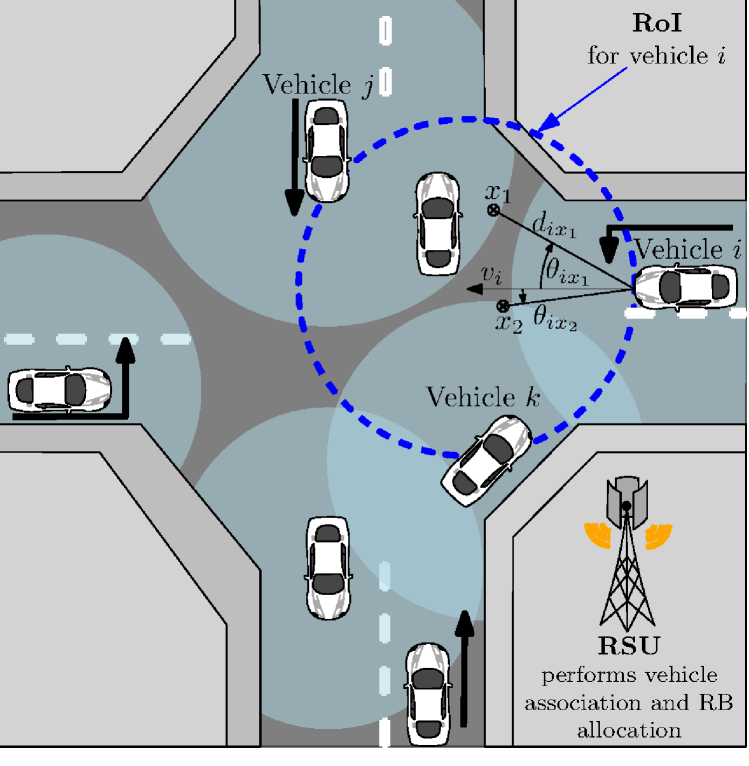
Figure 1: Vehicles under the coverage of a single RSU, drive through a junction while dynamically exchanging sensory information.

Consider a road junction covered and serviced by a single RSU, as shown in Fig. 1. We consider a time-slotted system with a slot index $t$ and a slot duration of $\tau$. Let $\mathcal{N}_{t}$ be the set of $N$ vehicles served by the RSU at time slot $t$, where $N$ is the maximum number of vehicles that could be served simultaneously by the RSU. We denote the location of each vehicle $n\in\mathcal{N}_{t}$ at time slot $t$ by $\boldsymbol{l}_{n}\left(t\right)$ and assume that each vehicle is equipped with a sensor having a fixed circular range of radius $r$. From a vehicle’s perspective, the output of the sensor regarding any location can have one of three states: Occupied ($s_{+}$), unoccupied ($s_{-}$), or unknown ($s_{0}$). The occupied state $s_{+}$ corresponds to locations within the vehicle’s sensing range where an obstacle is sensed. While, the unoccupied state $s_{-}$ corresponds to locations within the vehicle’s sensing range that are sensed to be obstacle-free. Finally, the unknown state $s_{0}$ corresponds to the locations which cannot be sensed by the vehicle’s sensor, either due to occlusions or because they are outside the vehicle’s sensing range. Lets assume that the output of vehicle $n$’s sensor regarding location $\boldsymbol{x}$ at time slot $t$ is $s_{n}(\boldsymbol{x},t)\in\{s_{+},s_{-},s_{0}\}$. Moreover, here the “ground-truth” state of any location $\boldsymbol{x}$ is either occupied $s_{+}$, or unoccupied $s_{-}$, and is given by $G(\boldsymbol{x},t)\in\{s_{+},s_{-}\}$. Since sensors are not perfectly reliable, then $s_{n}(\boldsymbol{x},t)$ will be correct, i.e., $s_{n}(\boldsymbol{x},t)=G(\boldsymbol{x},t)$, with a fixed probability of $\lambda_{n}$, where $\lambda_{n}\in(0.5,1]$ represents the sensor’s reliability. Thus, the probability of occupancy at location $\boldsymbol{x}$ with respect to vehicle $n$, given its sensor output, is,

$$p_{n}(\boldsymbol{x},t)=\text{Pr}(G(\boldsymbol{x},t)=s_{+}|s_{n}(\boldsymbol{x},t))=\begin{cases}\lambda_{n}&\text{if\leavevmode\nobreak\ }s_{n}(\boldsymbol{x},t)=s_{+},\\ 1-\lambda_{n}&\text{if\leavevmode\nobreak\ }s_{n}(\boldsymbol{x},t)=s_{-},\\ 1/2&\text{if\leavevmode\nobreak\ }s_{n}(\boldsymbol{x},t)=s_{0},\end{cases}$$ (1)

Note that, some locations are occluded by obstacles, or are outside the sensing range, which results in $s_{n}(\boldsymbol{x},t)=s_{0}$. In order to model the high uncertainty of this unknown state, it is mapped to $p_{n}(\boldsymbol{x},t)=\frac{1}{2}$ which represents the highest uncertainty in a probability distribution.

Let $q_{n}(\boldsymbol{x},t)$ be the value (or quality) of the sensed information at location $\boldsymbol{x}$ at the beginning of time slot $t.$ $q_{n}(\boldsymbol{x},t)$ depends on the probability of occupancy $p_{n}(\boldsymbol{x},t)$ and the age of the information (AoI) $\Delta_{n}(\boldsymbol{x},t)$ [34, 35], which is given by,

$$q_{n}(\boldsymbol{x},t)=|2p_{n}(\boldsymbol{x},t)-1|\mu^{\Delta_{n}(\boldsymbol{x},t)},$$ (2)

$$\Delta_{n}(\boldsymbol{x},t)=\tau t-\Gamma_{n}(\boldsymbol{x}),$$

with a parameter $\mu\in(0,1)$ and $\Gamma_{n}(\boldsymbol{x})$ defining the instant when $\boldsymbol{x}$ was last sensed by vehicle $n$. Here, we choose the AoI as a metric to emphasize the importance of fresh sensory information. Note that the value function $q_{n}(\boldsymbol{x})$ decreases as its AoI increases (outdated information) or the probability of occupancy for location $\boldsymbol{x}$ approaches 1/2 (uncertain information).

Moreover, each vehicle $n$ is interested in extending its sensing range. The higher the vehicle’s velocity is, the bigger this region of interest (RoI) should be. As a result, each vehicle is interested in $t_{\text{int}}$ seconds ahead along its direction of movement. The RoI of vehicle $n$, for simplicity, is captured by a circular region with a diameter of $v_{n}t_{\text{int}}$, where $v_{n}$ is the velocity of the vehicle. Within the RoI, the vehicle has higher interest in gaining sensory information regarding the locations closer to its current position as well as regarding locations closer to its direction of movement. Therefore, we formally define the interest of vehicle $n$ in location $\boldsymbol{x}$ as follows:

$$w_{n}(\boldsymbol{x})=\begin{cases}\frac{v_{n}t_{\text{int}}\cos\theta-d}{v_{n}t_{\text{int}}\cos\theta},&d\leq v_{n}t_{\text{int}}\cos\theta,\\ 0,&\text{o.w.},\end{cases},$$ (3)

where $d$ is the euclidean distance between the location $\boldsymbol{x}$ and the vehicle’s position $\boldsymbol{l}_{n}\left(t\right)$, and $\theta$ is the angle between the vehicle’s direction of motion and location $\boldsymbol{x}$, as illustrated in Fig. 1. To capture the need of gathering new information, the interest $w_{n}(\boldsymbol{x})$ of vehicle $n$ needs to be weighted based on the lack of worthy information, i.e., $1-q_{n}(\boldsymbol{x})$. Hence, the modified interest of vehicle $n$ in location $\boldsymbol{x}$ is given by,

$$i_{n}(\boldsymbol{x})=w_{n}(\boldsymbol{x})[1-q_{n}(\boldsymbol{x})].$$ (4)

We assume that each vehicle can associate with at most one vehicle at each time slot to exchange sensory information. We define $E(t)=\left[e_{nn^{\prime}}(t)\right]$ to be the global association matrix,where $e_{nn^{\prime}}(t)=1$ if vehicle $n$ is associated (transmits) to vehicle $n^{\prime}$ at time slot $t$, otherwise, $e_{nn^{\prime}}(t)=0$. It is assumed that the association is bi-directional, i.e., $e_{nn^{\prime}}(t)=e_{n^{\prime}n}(t)$. Moreover, we assume that each associated pair can communicate simultaneously with each other, i.e. each vehicle is equipped with two radios, one for transmitting and the other is for receiving. Additionally, a set $\mathcal{K}$ of $K$ orthogonal resource blocks (RBs), with bandwidth $\omega$ per RB, is shared among the vehicles, where each transmitting radio is allocated with only one RB. We further define $\eta_{nn^{\prime}}^{k}(t)\in\left\{0,1\right\}$, $\text{for all }k\in\mathcal{K}\text{ and }n,n^{\prime}\in\mathcal{N}$, as the RB allocation. Here, $\eta_{nn^{\prime}}^{k}(t)=1$ if vehicle $n$ transmits over RB $k$ to vehicle $n^{\prime}$ at time slot $t$ and $\eta_{nn^{\prime}}^{k}(t)=0$, otherwise. In order to avoid self-interference, the RBs allocated for each associated pair are orthogonal, i.e. $\eta_{nn^{\prime}}^{k}(t)\neq\eta_{n^{\prime}n}^{k}(t)$ given that $e_{nn^{\prime}}(t)=1$.

Let $h_{nn^{\prime}}^{k}(t)$ be the instantaneous channel gain, including path loss and channel fading, from vehicle $n$ to vehicle $n^{\prime}$ over RB $k$ in slot $t$. We consider the $5.9\text{ GHz}$ carrier frequency and adopt the realistic V2V channel model of [36] in which, depending on the location of the vehicles, the channel model is categorized into three types: line-of-sight, weak-line-of-sight, and non-line-of-sight. As a result, the data rate from vehicle $n$ to vehicle $n^{\prime}$ at time slot $t$ (in packets per slot) is expressed as

$$R_{nn^{\prime}}(t)=e_{nn^{\prime}}(t)\cdot\frac{\tau}{M}\sum_{k\in\mathcal{K}}\eta_{nn^{\prime}}^{k}(t)\omega\log_{2}\left(1+\frac{Ph_{nn^{\prime}}^{k}(t)}{N_{0}\omega+I_{nn^{\prime}}^{k}(t)}\right),$$ (5)

where $M$ is the packet length in bits, $P$ is the transmission power per RB, and $N_{0}$ is the power spectral density of the additive white Gaussian noise. Here, $I_{nn^{\prime}}^{k}(t)=\sum_{i,j\in\mathcal{N}/n,n^{\prime}}\eta_{i,j}^{k}(t)Ph_{in^{\prime}}^{k}(t)$ indicates the received aggregate interference at the receiver $n^{\prime}$ over RB $k$ from other vehicles transmitting over the same RB $k$.

II-A Quadtree Representation

Storing and exchanging raw sensory information between vehicles, e.g., information about individual locations $\boldsymbol{x}$, requires significant memory and communication resources for cooperative perception to be deemed useful. To alleviate this challenge, a compression technique called region quadtree, which efficiently store data on a two-dimensional space, can be used by each vehicle [20]. In this technique, each vehicle converts its sensing range into a squared-block of side-length $2r$. This block is divided recursively into 4 blocks until

• reaching a maximum resolution level $L$, or

• the state of every location $\boldsymbol{x}$ within a block is the same.

Without loss of generality, we assume that each block can be represented using $M$ bits. Fig. 2 shows the quadtree representation of the sensing range of vehicle $k$ with $L=5$.

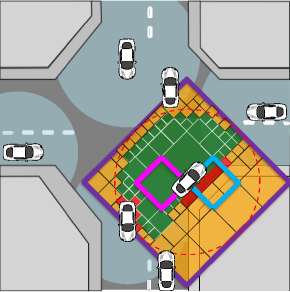
(a)	(b)

Figure 2: Quadtree representation of the sensing range of vehicle $k$, with a maximum resolution level $L=5$. Green represents the unoccupied state $s_{-}$, red represents the occupied state $s_{+}$ and orange represents the unknown state $s_{0}$. (a) shows the block decomposition of the sensing range while (b) shows the equivalent tree diagram. The block with purple boarders represents the lowest resolution block that can be transmitted. Another two examples of different blocks are highlighted in the same way using pink and blue boarders.

The state of block $b$ within the quadtree of vehicle $n$ is either,

• Occupied: If the state of any location $\boldsymbol{x}$ within the block is occupied,

• Unoccupied: If every location within the block is unoccupied,

• Unknown: Otherwise.

In this view, the probability of occupancy of each block $p_{n}(b)$ can be defined in the same manner as (1):

$$p_{n}(b)=\begin{cases}\lambda_{n}&\text{if\leavevmode\nobreak\ }s_{n}(b)=s_{+},\\ 1-\lambda_{n}&\text{if\leavevmode\nobreak\ }s_{n}(b)=s_{-},\\ 1/2&\text{if\leavevmode\nobreak\ }s_{n}(b)=s_{0},\end{cases}$$ (6)

and the worthiness of block $b$’s sensory information $q_{n}(b)$ is defined in the same manner as (2).

Let $\mathcal{B}_{n}\left(t\right)$ represent the set of quadtree blocks available for transmission by vehicle $n$ at the beginning of time slot $t$. Assume that $\mathcal{B}_{n}\left(t\right)=\mathcal{B}_{n}^{\text{c}}\cup\mathcal{B}_{n}^{\text{p}}$, where $\mathcal{B}_{n}^{\text{c}}$ is the set of blocks available from its own current sensing range, while $\mathcal{B}_{n}^{\text{p}}$ is the set of blocks available from previous slots (either older own blocks or blocks received from other vehicles). Note that, due to the quadtree compression, the cardinality of $\mathcal{B}_{n}^{\text{c}}$ is upper bounded by: $|\mathcal{B}_{n}^{\text{c}}|\leq\sum_{l=0}^{L-1}4^{l}=\frac{1-4^{L}}{1-4}$. Also, in order to keep the exchanged sensory information fresh, an upper bound is applied on the cardinality of $\mathcal{B}_{n}^{\text{p}}$: $|\mathcal{B}_{n}^{\text{p}}|\leq B_{\text{max}}^{\text{p}}$, where blocks with higher AoI are discarded if the cardinality of $\mathcal{B}_{n}^{\text{p}}$ exceeded $B_{\text{max}}^{\text{p}}$. Determining what quadtree blocks needs to be shared, and with which vehicles, is not straightforward. In order to answer those questions, we first start by formulating the problem.

III Problem Formulation

In our model, each vehicle $n$ is interested in associating (pairing) with another vehicle $n^{\prime}$ where each pair exchanges sensory information in the form of quadtree blocks with the objective of maximizing the joint satisfaction of both vehicles. The satisfaction of vehicle $n$ with the sensory information received from vehicle $n^{\prime}$ at time slot $t$ can be defined as follows:

$$f_{nn^{\prime}}\left(t\right)=\sum_{b\in\mathcal{B}_{n^{\prime}}\left(t\right)}\sigma_{n^{\prime}}^{b}\left(t\right)\left(\frac{\sum_{\boldsymbol{x}\in b}i_{n}\left(\boldsymbol{x}\right)}{\Lambda\left(b\right)}.q_{n^{\prime}}\left(b\right)\right),$$ (7)

where $\sigma_{n^{\prime}}^{b}\left(t\right)=1$ if vehicle $n^{\prime}$ transmitted block $b$ to vehicle $n$ at time slot $t$, and $\sigma_{n^{\prime}}^{b}\left(t\right)=0$ otherwise, and $\Lambda\left(b\right)$ is the area covered by block $b$. Moreover, it should be noted that vehicle $n$ is more satisfied with receiving quadtree blocks with a resolution proportional to the weights of its RoI as per (4), i.e., block $b$ with higher resolution (smaller coverage area $\Lambda\left(b\right)$) for the regions with higher $i_{n}\left(\boldsymbol{x}\right)$, which is captured by $\frac{\sum_{\boldsymbol{x}\in b}i_{n}\left(\boldsymbol{x}\right)}{\Lambda\left(b\right)}$. Furthermore, vehicle $n$ is more satisfied with receiving quadtree blocks having more worthy sensory information, which is captured by $q_{n^{\prime}}\left(b\right)$. As a result, our cooperative perception network-wide problem can be formally posed as follows:

$$\max_{\boldsymbol{\eta}(t),E(t),\boldsymbol{\sigma}\left(t\right)} \leavevmode\nobreak\ \leavevmode\nobreak\ \sum\limits_{n,n^{\prime}\in\mathcal{N}}f_{nn^{\prime}}\left(t\right)\cdot f_{n^{\prime}n}\left(t\right)$$

s.t. $$\leavevmode\nobreak\ \leavevmode\nobreak\ \sum_{b\in\mathcal{B}_{n}\left(t\right)}\sigma_{n}^{b}\left(t\right)\leq\sum_{n^{\prime}\in\mathcal{N}}R_{nn^{\prime}}(t),\ \forall n\in\mathcal{N},\,\forall t,$$ (8a)

$$\leavevmode\nobreak\ \leavevmode\nobreak\ {\textstyle\sum\limits_{n^{\prime}\in\mathcal{N}}}\sum_{k\in\mathcal{K}}\eta_{nn^{\prime}}^{k}(t)\leq 1,\leavevmode\nobreak\ \forall n\in\mathcal{N},\,\forall t,$$ (8b)

$$\leavevmode\nobreak\ \leavevmode\nobreak\ \sum_{n^{\prime}\in\mathcal{N}}e_{nn^{\prime}}\left(t\right)\leq 1,\ \forall n\in\mathcal{N},\,\forall t,$$ (8c)

$$\ \ e_{nn^{\prime}}\left(t\right)=e_{n^{\prime}n}\left(t\right),\ \forall n,n^{\prime}\in\mathcal{N},\,\forall t,$$ (8d)

$$\leavevmode\nobreak\ \leavevmode\nobreak\ \eta_{nn^{\prime}}^{k}(t)\in\{0,1\},e_{nn^{\prime}}\left(t\right)\in\left\{0,1\right\},\sigma_{n}^{b}\left(t\right)=\left\{0,1\right\}\leavevmode\nobreak\ \forall t,\,k\in\mathcal{K},\,n,n^{\prime}\in\mathcal{N},$$ (8e)

where the objective is to associate vehicles $E\left(t\right)$, allocate RBs $\boldsymbol{\eta}\left(t\right)=[\eta_{nn^{\prime}}^{k}(t)]^{k\in\mathcal{K}}_{n,n^{\prime}\in\mathcal{N}}$, and select the contents of the transmitted messages (the quadtree blocks to be transmitted by each vehicle) $\boldsymbol{\sigma}\left(t\right)$, in order to maximize the sum of the joint satisfaction of the associated vehicular pairs. Note that (8a) is an upper bound on the number of transmitted quadtree blocks of each vehicle by its Shannon data rate, while (8b) constrains the number of RBs allocated to each vehicle to 1.

Note that, the RB allocation $\eta_{nn^{\prime}}^{k}(t)$ and the vehicular association $E\left(t\right)$ directly determine the data rate $R_{nn^{\prime}}(t)$ as per (5), specifying the maximum number of quadtree blocks to be transmitted between the vehicles. Moreover, the selected quadtree blocks $\boldsymbol{\sigma}\left(t\right)$ along with $E\left(t\right)$ directly determines the vehicular satisfaction as per (7). As a result finding the optimal solution (RB allocation, vehicular association and message content selection) of this problem is complex and not straightforward. From a centralized point of view where the RSU tries to solve this problem, the RSU needs to know the real-time wireless channels between the vehicles and the details of the sensed information of each vehicle, in order to optimally solve (8). Frequently exchanging such fast-varying information between the RSU and vehicles can yield a huge communication overhead which is impractical. From a decentralized point of view, in order to maximize (7), vehicle $n^{\prime}$ needs to know the exact interest of vehicle $n$ as per (4) in order to optimally select the quadtree blocks to be transmitted, which is impractical as well. Hence, to solve (8) we leverage machine learning techniques which have proved to be useful in dealing with such complex situations, specifically DRL [29].

IV Reinforcement Learning Based Cooperative Perception

IV-A Background

RL is a computational approach to understanding goal-directed learning and decision-making [37]. RL is about learning from interactions how to behave in order to achieve a goal. The learner (or decision-maker) is called an agent who interacts with the environment, which is comprising everything outside the agent.

Thus, any goal-directed learning problem can be reduced to three signals exchanged between an agent and its environment: one signal representing the choices made by the agent (actions), one signal representing the basis on which the choices are made (states), and one signal defining the agent’s goal (rewards). In a typical RL problem, the agent’s goal is to maximize the total amount of reward it receives, which means maximizing not just the immediate reward, but a cumulative reward in the long run.

RL problems are typically formalized using Markov decision processes (MDPs) [37], characterized as $\left\langle\mathcal{S},\mathcal{A},\mathcal{T},\mathcal{R},\gamma\right\rangle$. That is, at timestep $t$, the agent with state $s\in\mathcal{S}$ performs an action $a\in\mathcal{A}$ using a policy $\pi\left(a|s\right)$, and receives a reward $r_{t}=\mathcal{R}\left(s,a\right)\in\mathbb{R}$, and transitions to state $s^{\prime}\in\mathcal{S}$ with probability $p\left(s^{\prime}|s,a\right)=\mathcal{T}\left(s,a,s^{\prime}\right)$. We define $R_{t}=\sum_{t^{\prime}=t}^{H}\gamma^{t^{\prime}-t}r_{t}$ as the discounted return over horizon $H$ and discount factor $\gamma\in\left[0,1\right)$, and we define $Q^{\pi}\left(s,a\right)=\mathbb{E}_{\pi}\left[R_{t}|s_{t}=s,a_{t}=a\right]$ as the action-value (Q-value) of state $s$ and action $a$. Moreover, let $\pi^{*}$ be the optimal policy that maximizes the Q-value function, $Q^{\pi^{*}}\left(s,a\right)=\max_{\pi}Q^{\pi}\left(s,a\right)$. The ultimate goal of RL is to learn the optimal policy $\pi^{*}$ by having agents interacting with the environment.

Among the various techniques used to solve RL problems, in this work we will advocate for the use of Q-learning and deep Q-networks (DQNs).

IV-A1 Q-learning and DQNs

Q-learning iteratively estimates the optimal Q-value function, $Q\left(s,a\right)=Q\left(s,a\right)+\alpha\left[r+\gamma\max_{a^{\prime}}Q\left(s^{\prime},a^{\prime}\right)-Q\left(s,a\right)\right]$, where $\alpha\in\left[0,1\right)$ is the learning rate and $\left[r+\gamma\max_{a^{\prime}}Q\left(s^{\prime},a^{\prime}\right)-Q\left(s,a\right)\right]$ is the temporal-difference (TD) error. Convergence to $Q^{\pi^{*}}$ is guaranteed in the tabular (no approximation) case provided that sufficient state/action space exploration is done; thus, tabulated learning is not suitable for problems with large state spaces. Practical TD methods use function approximators for the Q-value function such as neural networks, i.e., deep Q-learning which exploits Deep Q-Networks (DQNs) for Q-value approximation [29].

RL can be unstable or even diverge when a nonlinear function approximator such as a neural network is used to represent the Q-value function [38]. In order to overcome this issue, DQNs rely on two key concepts, the experience replay and an iterative update that adjusts the Q-values towards target values that are only periodically updated.

The approximate Q-value function is parameterized using a deep neural network, $Q\left(s,a;\phi\right)$, in which $\phi$ are the parameters (weights) of the Q-network. To use experience replay, the agent’s experiences $\mu_{t}=\left(s_{t},a_{t},r_{t},s_{t+1}\right)$ are stored at each timestep $t$ in a data set $\mathcal{D}_{t}=\left\{\mu_{1},\cdots,\mu_{t}\right\}$. During learning, Q-learning updates are applied on samples (minibatches) of experience $\left(s,a,r,s^{\prime}\right)\sim U\left(\mathcal{D}\right)$, drawn uniformly at random from the pool of stored samples. The Q-learning update uses the following loss function:

$$L\left(\phi\right)=\mathbb{E}_{\left(s,a,r,s^{\prime}\right)\sim U\left(\mathcal{D}\right)}\left[\left(r+\gamma\max_{a^{\prime}}Q\left(s^{\prime},a^{\prime};\phi^{-}\right)-Q\left(s,a;\phi\right)\right)^{2}\right],$$

where $\phi^{-}$ are the network parameters used to compute the target. The target network parameters $\phi^{-}$ are only updated with the Q-network parameters $\phi$ every $C$ steps and remain fixed across individual updates [29].

IV-B Cooperative Perception Scenario

In order to solve (8), the timeline is splitted into two scales, a coarse scale called time frames and a fine scale called time slots. At the beginning of each time frame, the RSU associates vehicles into pairs and allocates RBs to those pairs. The association and RB allocation stays fixed during the whole frame which consists of $X$ time slots. At the beginning of each time slot $t$, each vehicle selects the quadtree blocks to be transmitted to its associated vehicle. By utilizing RL we can formulate two different but interrelated RL problems: Vehicular RL and RSU RL.

IV-B1 Vehicular RL

In this RL problem, for a given association $nn^{\prime}$ and RB allocation, each vehicle $n$ acts as an RL-agent who wants to learn which quadtree blocks to transmit to its associated vehicle $n^{\prime}$ in order to maximize the satisfaction of vehicle $n^{\prime}$. Accordingly, the global state of the RL environment is defined as $\left\langle\mathcal{B}_{n}\left(t\right),\mathcal{I}_{n^{\prime}}(t),v_{n},v_{n^{\prime}},\boldsymbol{l}_{n}\left(t\right),\boldsymbol{l}_{n^{\prime}}\left(t\right)\right\rangle$, where $\mathcal{I}_{n^{\prime}}\left(t\right)$ is the set of vehicle’s $n^{\prime}$ RoI weights, as per (4), at time slot $t$. However, this global state cannot be observed by vehicle $n$, where instead, the local observation of vehicle $n$ is $\left\langle\mathcal{B}_{n}\left(t\right),v_{n},v_{n^{\prime}},\boldsymbol{l}_{n}\left(t\right),\boldsymbol{l}_{n^{\prime}}\left(t\right)\right\rangle$. At every time slot $t$ and by utilizing this local observation, vehicle $n$ takes an action $\boldsymbol{\sigma}_{n}\left(t\right)$, selecting which quadtree blocks to be transmitted to its associated vehicle $n^{\prime}$, and accordingly receive a feedback (reward) from vehicle $n^{\prime}$ equal to $f_{n^{\prime}n}\left(t\right)$. In a nutshell, the elements of the RL problem at each vehicle $n$ can be described as follows:

• Global state: $\left\langle\mathcal{B}_{n}\left(t\right),\mathcal{I}_{n^{\prime}}(t),v_{n},v_{n^{\prime}},\boldsymbol{l}_{n}\left(t\right),\boldsymbol{l}_{n^{\prime}}\left(t\right)\right\rangle$.

• Local observation: $\left\langle\mathcal{B}_{n}\left(t\right),v_{n},v_{n^{\prime}},\boldsymbol{l}_{n}\left(t\right),\boldsymbol{l}_{n^{\prime}}\left(t\right)\right\rangle$.

• Action: $\boldsymbol{\sigma}_{n}\left(t\right)$.

• Reward: $f_{n^{\prime}n}\left(t\right)$.

IV-B2 RSU RL

The RSU acts as an RL-agent where the state of this RL environment is given by the location and velocity of all vehicles serviced by the RSU, $\left\langle v_{n},\boldsymbol{l}_{n}\,\forall n\in\mathcal{N}\right\rangle$. Based on this state at the beginning of each time frame, the RSU takes the action of vehicles association $E(t)$, and RB allocation $\boldsymbol{\eta}(t)$. Then, once the time frame ends, each vehicle will report back its mean satisfaction during the whole frame and the RL reward is computed as the mean of those feedbacks. In a nutshell, the elements of the RL problem at the RSU can be summarized as follows:

• State: $\left\langle v_{n},\boldsymbol{l}_{n}\,\forall n\in\mathcal{N}\right\rangle$.

• Action: $E(t)$ and $\boldsymbol{\eta}(t)$.

• Reward: $\frac{\sum_{n\in\mathcal{N}}\nicefrac{{\left(\sum_{t=i}^{i+X}f_{n^{\prime}n}\left(t\right)\right)}}{{X}}}{|\mathcal{N}|}$.

In order to solve these two RL problems, the DQN algorithm [29] can be used. However, despite its success in domains with high-dimensional state space such as our domain, its application to high dimensional, discrete action spaces is still arduous, because within DQN, the Q-value for each possible action should be estimated before deciding which action to take. Furthermore, the number of actions that need to be explicitly represented grows exponentially with increasing action dimensionality [33].

At this point, we note that our two RL problems suffer from the high dimensionality of action spaces. Specifically, within the RSU RL problem, the RSU needs to select $E(t)$ and $\boldsymbol{\eta}(t)$: The association matrix $E(t)$ is of size $N\times N$, and due to our one-to-one association assumption, the number of possible actions for the association problem would be $\Pi_{n=1}^{\left\lfloor\nicefrac{{N}}{{2}}\right\rfloor}\left(2n-1\right)$. Moreover, the RB allocation matrix $\boldsymbol{\eta}(t)$ is of size $N\times K$, as a result, the number of possible actions is $K^{N}$, assuming that each vehicle is allocated only 1 RB. Similarly, within the vehicular RL problem, each vehicle needs to select $\boldsymbol{\sigma}_{n}\left(t\right)$ whose dimension is $|\mathcal{B}_{n}|_{\text{max}}\times 1$, yielding a total number of possible actions equal to $2^{|\mathcal{B}_{n}|_{\text{max}}}$.

This large number of actions can seriously affect the learning behavior of the available discrete-action reinforcement learning algorithms such as DQN, because large action spaces are difficult to explore efficiently and thus successful training of the neural networks becomes intractable [39].

V Overcoming the Large Action Space Problem

Recently, the authors in [33] have introduced a new agent called branching dueling Q-network (BDQ). The resulting neural network architecture allows to distribute the representation of the action dimensions across individual network branches while maintaining a shared module that encodes a latent representation of the input state and helps to coordinate the branches. This architecture is represented in Fig. 3. Remarkably, this neural network architecture exhibits a linear growth of the network outputs with increasing action space as opposed to the combinatorial growth experienced in traditional DQN network architectures.

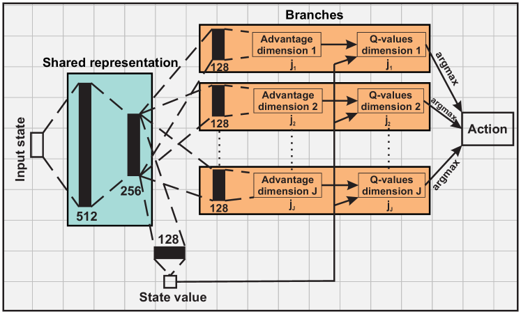
Figure 3: The BDQ neural network architecture utilized for both RSU and vehicular RL agents.

Here, we adopt these BDQ agents from [33] within our RL problems. As a result, the neural network at the RSU agent will have $N$ branches constructed as follows:

• $\left\lfloor\nicefrac{{N}}{{2}}\right\rfloor$ branches corresponding to the association action with each branch having $j_{i}=N-2i+1$ sub-actions, where $i$ is the branch ID. For example, let us consider a simplified scenario with $N=6$, then $\left\lfloor\nicefrac{{N}}{{2}}\right\rfloor=3$ vehicular pairs could be formed: the first branch representing the first vehicle would have $N-2\cdot(1)+1=5$ candidate vehicles to pair with, while for the second branch the candidates are reduced to 3 and so on. This leads to a unique vehicular association for any combination of sub-actions selected at each of the branches. For instance, an action of $(1,1,1)$ implies that $E=\left[\begin{array}[]{cccccc}0&1&0&0&0&0\\ 1&0&0&0&0&0\\ 0&0&0&1&0&0\\ 0&0&1&0&0&0\\ 0&0&0&0&0&1\\ 0&0&0&0&1&0\end{array}\right],$ and an action of $(3,2,1)$ would mean that $E=\left[\begin{array}[]{cccccc}0&0&0&1&0&0\\ 0&0&0&0&1&0\\ 0&0&0&0&0&1\\ 1&0&0&0&0&0\\ 0&1&0&0&0&0\\ 0&0&1&0&0&0\end{array}\right]$.

• $\left\lfloor\nicefrac{{N}}{{2}}\right\rfloor$ branches corresponding to the RB allocation with each branch having ${K\choose 2}$ sub-actions, knowing that each associated pair is allocated 2 orthogonal RBs (one for each vehicle).

The aftermath of using the BDQ agent is that, in order to select an association action $E(t)$, the Q-value needs to be estimated for $\sum_{n=1}^{\left\lfloor\nicefrac{{N}}{{2}}\right\rfloor}\left(2n-1\right)$ actions instead of for $\Pi_{n=1}^{\left\lfloor\nicefrac{{N}}{{2}}\right\rfloor}\left(2n-1\right)$ with a non-branching network architecture. Similarly, selecting an RB allocation $\boldsymbol{\eta}(t)$, requires the Q-value estimation of $\frac{N}{2}\times{K\choose 2}$ actions instead of the ${K\choose 2}^{\nicefrac{{N}}{{2}}}$values involved in a traditional DQN architecture. Equivalently, by utilizing the BDQ agent within our vehicular RL problem, for the message content selection $\boldsymbol{\sigma}_{n}\left(t\right)$, the Q-value needs to be estimated for $2\times|\mathcal{B}_{n}|_{\text{max}}$ actions only instead of for $2^{|\mathcal{B}_{n}|_{\text{max}}}$ actions.

V-A Training a BDQ Agent within The Cooperative Perception Scenario

For training the RSU and vehicular agents, DQN is selected as the algorithmic basis. Thus, at the beginning of each RSU episode, a random starting point of an arbitrary trajectory of vehicles is selected, resulting in a an indiscriminate state $\left\langle v_{n},\boldsymbol{l}_{n}\,\forall n\in\mathcal{N}\right\rangle$ observed by the RSU. Here, this state is the input to the BDQ agent (neural network) available at the RSU. Then, with probability $\epsilon$, this BDQ agent randomly selects the association $E\left(t\right)$ and RB allocation $\boldsymbol{\eta}(t)$ actions, and with probability $1-\epsilon$, it will select the action having the maximum Q-value (as determined by the output of the neural network).

For any action dimension $i\in\left\{1,\dots,J\right\}$ with $\left|\mathcal{A}_{i}\right|=j_{i}$ discrete sub-actions, the Q-value of each individual branch at state $s\in\mathcal{S}$ and sub-action $a_{i}\in\mathcal{A}_{i}$ is expressed in terms of the common state value $V\left(s\right)$ and the corresponding state-dependent sub-action advantage $A_{i}\left(s,a_{i}\right)$ by [33]:

$$Q_{i}\left(s,a_{i}\right)=V\left(s\right)+\left(A_{i}\left(s,a_{i}\right)-\frac{1}{j_{i}}\sum_{a^{\prime}_{i}\in\mathcal{A}_{i}}A_{i}\left(s,a^{\prime}_{i}\right)\right).$$ (9)

After the action is determined, the RSU forwards the association and RB allocation decision to the corresponding vehicles. This association and RB allocation decision will hold for the upcoming $X$ time slots. Once the RSU decision has been conveyed to the vehicles, each vehicle $n$ can compute its local observation $\left\langle\mathcal{B}_{n}\left(t\right),v_{n},v_{n^{\prime}},\boldsymbol{l}_{n}\left(t\right),\boldsymbol{l}_{n^{\prime}}\left(t\right)\right\rangle$. Note here that, this local observation constitutes the input for the BDQ agent running at vehicle $n$. Furthermore, an $\epsilon-$greedy policy is also employed at each vehicle, thus random sensory blocks will be selected for transmission with probability $\epsilon$, and the sensory blocks which maximizes the Q-value with probability $1-\epsilon$. Then, the resulting sensory blocks will be scheduled for transmitted over the allocated RB to the associated vehicle. Notice that, the associated vehicle might only receive a random subset of these blocks depending on the data rate $R_{nn^{\prime}}\left(t\right)$ as per (5). It will then calculate its own satisfaction $f_{n^{\prime}n}\left(t\right)$ with the received blocks according to (7) and feed this value back as a reward to vehicle $n$. Vehicle $n$ receives the reward, observes the next local observation and stores this experience $\mu_{t}^{n}=\left(s_{t},a_{t},r_{t},s_{t+1}\right)$ in a data set $\mathcal{D}_{t}^{n}=\left\{\mu_{1}^{n},\cdots,\mu_{t}^{n}\right\}$. After $X$ time slots, each vehicle will feedback its average received reward during the whole frame to the RSU that will calculate the mean of all the received feedbacks and use the result as its own reward for the association and RB allocation action. The RSU stores its own experience, $\mu_{m}^{\text{RSU}}=\left(s_{m},a_{m},r_{m},s_{m+1}\right)$, in a data set $\mathcal{D}_{m}^{\text{RSU}}=\left\{\mu_{1}^{\text{RSU}},\cdots,\mu_{m}^{\text{RSU}}\right\}$, where $m$ is the frame index. A new RSU episode begins every $Z$ frames.

Once an agent has collected a sufficient amount of experience, the training process of its own neural network starts. First, samples of experience (mini-batch) are drawn uniformly at random from the pool of stored samples, $\left(s,a,r,s^{\prime}\right)\sim U\left(\mathcal{D}\right)$ . Using these samples, the loss function within the branched neural network architecture of the BDQ agent is calculated as follows [33]:

$$L\left(\phi\right)=\mathbb{E}_{\left(s,a,r,s^{\prime}\right)\sim U\left(\mathcal{D}\right)}\left[\frac{1}{J}\sum_{i}\left(y_{i}-Q_{i}\left(s,a_{i}\right)\right)^{2}\right],$$ (10)

where $i$ is the branch ID, $J$ is the total number of branches, and $a$ denotes the joint-action tuple $\left(a_{1},\cdots,a_{i},\cdots,a_{J}\right)$. Moreover, $y_{i}=r+\gamma\frac{1}{J}\sum_{i}Q_{i}^{-}\left(s^{\prime},\text{arg max}_{a^{\prime}_{i}\in\mathcal{A}_{i}}Q_{i}\left(s^{\prime},a^{\prime}_{i}\right)\right)$ in (10) represents the temporal difference targets. Finally, a gradient descent step is performed on $L\left(\phi\right)$ with respect to the network parameters $\phi$. The training process of the BDQ agents is summarized in Algorithm 1.

1:  Initialize the replay memory of each agent to a fixed buffer size.

2:  Initialize each agent’s neural network with random weights $\phi$.

3:  Initialize each agent’s target neural network with weights $\phi^{-}=\phi$.

4:  foreach RSU episode do

5:     Reset the RSU environment by selecting random trajectories for all vehicles within the junction scenario.

6:     The RSU observes its current state $\left\langle v_{n},\boldsymbol{l}_{n}\,\forall n\in\mathcal{N}\right\rangle$.

7:     foreach $Z$ frames do

8:        With probability $\epsilon$, the RSU agent selects a random association and RB allocation action, otherwise the action with maximum Q-value is selected.

9:        This action (decision) is forwarded to the corresponding vehicles.

10:        foreach $X$ slots at each vehicle do

11:           Vehicle $n$ computes its local observation $\left\langle\mathcal{B}_{n}\left(t\right),v_{n},v_{n^{\prime}},\boldsymbol{l}_{n}\left(t\right),\boldsymbol{l}_{n^{\prime}}\left(t\right)\right\rangle$.

12:           With probability $\epsilon$, it selects random sensory blocks to be transmitted to its associated vehicle, otherwise the sensory blocks with maximum Q-value are selected.

13:           Transmit over the allocated RB to the associated vehicle; As per rate $R_{nn^{\prime}}\left(t\right)$ in (5) only a random subset of these blocks will be received.

14:           It calculates its own satisfaction $f_{nn^{\prime}}\left(t\right)$ as per (7) and feeds it back as a reward to the associated vehicle.

15:           Receive the reward, observe the next local observation and store this experience $\left(s_{t},a_{t},r_{t},s_{t+1}\right)$ in its replay memory.

16:           if vehicle $n$ has collected a sufficient amount of experiences do

17:              Vehicle $n$ samples uniformly a random mini-batch of experiences $\mu^{n}$ from its replay memory.

18:              It performs a gradient decent step on $L\left(\phi\right)$ w.r.t. $\phi$, using the samples.

19:           end if

20:        end for

21:        Each vehicle feeds back its average received reward during the whole frame to the RSU.

22:        The RSU calculates the mean of all the received feedbacks and use the result as its own reward.

23:        The RSU stores its own experience, $\left(s_{i},a_{i},r_{i},s_{i+1}\right)$, in its replay memory.

24:        if the RSU collected a sufficient amount of experiences do

25:           Sample uniformly a random mini-batch of experiences from its replay memory.

26:           Using these samples, a gradient decent step is performed on $L\left(\phi\right)$ w.r.t. $\phi$.

27:        end if

28:     end for

29:  end for

Algorithm 1 Training a BDQ agent for cooperative perception

VI Federated RL

We now observe that, so far, each vehicle $n$ has only leveraged its own experience to train its BDQ agent independently. Therefore, in order to have a resilient agent that performs well in different situations, the training process should run for a sufficient amount of time for the vehicle to gain a broad experience. Alternatively, vehicles could periodically share their trained models with each other to enhance the training process and obtain a better model in a shorter amount of time.

For that purpose, we investigate the role of federated RL [30] where different agents (vehicles) collaboratively train a global model under the orchestration of a central entity (RSU), while keeping the training data (experiences) decentralized [40, 41]. Instead of applying federated learning (FL) within a supervised learning task, in this work, we investigate the use of FL for reinforcement learning within our cooperative perception vehicular RL problem. In particular, at the end of every time frame $m$, each vehicle $n$, under the service of the RSU, updates (trains) its local model (neural network weights) $\phi_{m}^{n}$ based on its local experiences, by performing a gradient descent step on $L\left(\phi_{m}^{n}\right)$ as per (10). Next, each vehicle shares this updated model with the RSU which computes a global model by aggregating all the received models as follows:

$$\phi_{m}^{*}=\frac{1}{N}\sum_{n}\phi_{m}^{n},$$

where $\phi_{m}^{*}$ is the global model computed by the RSU at time frame $m$. After computing the global model, the RSU broadcasts $\phi_{m}^{*}$ back to the vehicles under its service, where each vehicle replaces its local model with $\phi_{m}^{*}$. Algorithm 2 summarizes the entire FRL process within our cooperative perception scenario.

1:  foreach frame $m$ do

2:     At each vehicle $n$ served by the RSU

3:        Perform a gradient descent step on $L\left(\phi_{m}^{n}\right)$ as per (10).

4:        Update the local model $\phi_{m}^{n}$.

5:        Share $\phi_{m}^{n}$ with the RSU.

6:     At the RSU

7:        Aggregate the received models according to $\phi_{m}^{*}=\frac{1}{N}\sum_{n}\phi_{m}^{n}$.

8:        Broadcast $\phi_{m}^{*}$ back to the vehicles.

9:  end for

Algorithm 2 FRL for vehicular cooperative perception

VII Simulation Results and Analysis

Simulations are conducted based on practical traffic data to demonstrate the effectiveness of the proposed approach. A traffic light regulated junction scenario is considered. Several junction scenes of random vehicles’ mobility traces were generated using the Simulation of Urban MObility (SUMO) framework [42]. Each scene spans a $30000$ time slots and consists of a total of 30 vehicles entering and exiting the coverage area of a single RSU. The vehicles are of different dimensions to mimic assorted cars, buses, and trucks. Unless stated otherwise, the simulation parameters are listed in Table I.

Table I: Simulation parameters.

Parameter	Value	Parameter	Value
$K$	$10$	$N_{0}$	$-174$ dBm/Hz
$\omega$	$180$ kHz	$P$	$10$ dBm
$\tau$	$2$ ms	$t_{\text{int}}$	$2$ sec
$M$	$100$ bytes	$L$	5
$\lambda_{n}$	1	$r$	20
$X$	$5$ slots	$Z$	$10$ frames

Moreover, the hyperparameters used for training the RSU and vehicular agents are discussed next. Common to all agents, training always starts after the first $1000$ simulation steps; subsequently, for each simulation time step a training step will be run. Adam optimizer is used with a learning rate of $10^{-4}$. Training is performed with a minibatch size of $64$ and a discount factor $\gamma=0.99$. In addition, the target network is updated every $1000$ time steps. A rectified non-linearity (ReLU) is used for all hidden layers and a linear activation is used on the output layers, for all neural networks. Each neural network is comprised of two hidden layers with $512$ and $256$ units in the shared network module and of one hidden layer per branch with $128$ units. Finally, a buffer size of $10^{6}$ is set for the replay memory of each agent.

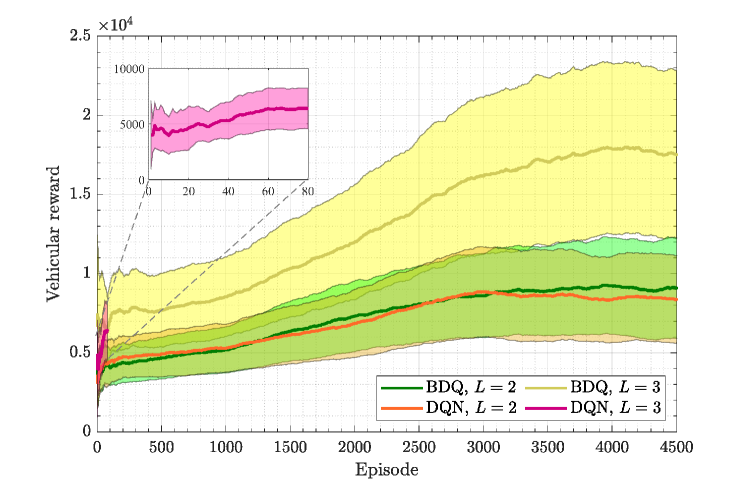
Figure 4: Learning curves for the vehicular RL environment. The solid lines represent the average over all the vehicles, where the learning curve of each vehicle is smoothed by the moving average over a window size of 1000 episodes, while the shaded areas show the 90% confidence interval over the vehicles.

First of all, we verify whether the BDQ agent is able to deal with the huge action space problem without experiencing any notable performance degradation when compared to a classical DQN agent. For this purpose, we alter the size of the action space of the vehicular RL problem by increasing the maximum quadtree resolution $L$. Note that, when $L=2,$ the maximum number of blocks available is $\frac{1-4^{L}}{1-4}=5$, resulting in a total number of actions of $2^{5}=32$, whereas when $L=3$, the maximum number of blocks available is $21$, leading to a total number of $2^{21}\thickapprox 2\times 10^{6}$ actions, assuming that each vehicle $n$ only transmits blocks within its $\mathcal{B}_{n}^{\text{c}}$. Fig. 4 shows the learning curve of both BDQ and DQN agents, for each case of $L$. When $L=2$ (small action space), the learning curves of both BDQ and DQN agents are comparable and they learn with the same rate. However, when $L$ increases to $3$ (large action space), the training process of the DQN agent could not be completed because it was computationally expensive. This is due to the large number of actions that need to be explicitly represented by the DQN network and hence, the extreme number of network parameters that must be trained at every iteration. The BDQ agent, however, performs well and shows robustness against huge action spaces, which demonstrates its suitability to overcome the scalability problems faced by other forms of RL.

Figure 5: Training and evaluation curves of the non-Federated scenario for the RSU agent for different $N$. Each line is smoothed by the moving average over a window size of 500 episodes.

Next, in Fig. 5, we study the training progress of the RSU agent within the non-federated scenario for different values of $N$, where $N$ is the maximum number of vehicles that could be served by the RSU. Fig. 5 demonstrates how the RSU reward increases gradually with the number of training episodes, i.e., the RSU and vehicles learn a better association, RB allocation and message content selection over the training period. However, it can be noted that the rate of increase of the RSU reward decreases as the number of served vehicles $N$ increases and, hence, more episodes are required to reach the same performance. The latter is motivated by the inflation in the state space of the RSU agent, which would require more episodes to be explored. Moreover, evaluations were conducted every 100 episodes of training for 10 episodes with a greedy policy. Fig. 5 shows the progress of the evaluation process during training and verifies that agents learn better policies along the training duration.

In Fig. 6, we compare the evolution of the training process both for the federated and non-federated scenarios, and for different values of $N$. From this figure, we observe that for the same training period, if compared to the non-federated scenario, the federated scenario achieves better rewards, and, hence, better policies over all vehicles. This result corroborates that FL algorithms are instrumental in enhancing and boosting the RL training process.

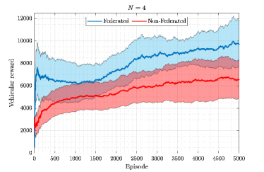
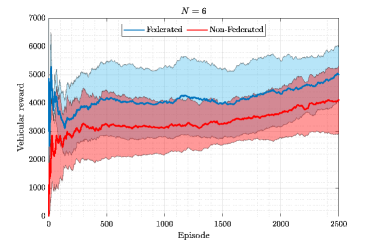
(a)	(b)
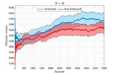
(c)

Figure 6: Learning curves for the federated vs non-federated scenarios of vehicular cooperative perception environment with $L=5$. The solid lines represent the average over all the vehicles, where the learning curve of each vehicle is smoothed by the moving average over a window size of 1000 episodes, while the shaded areas show the 90% confidence interval over the vehicles.

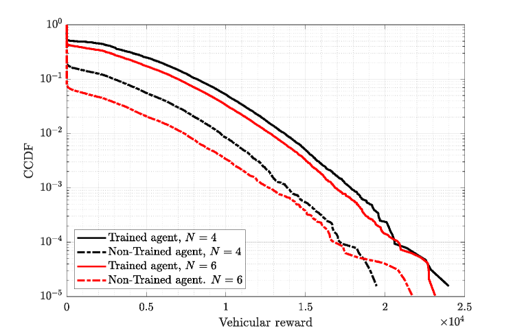
Figure 7: The CCDF of the vehicular reward achieved by trained and non-trained agents for different $N$.

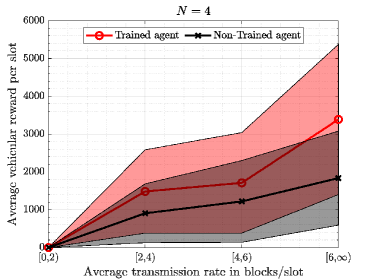
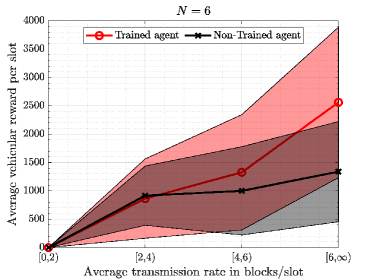
(a)	(b)

Figure 8: The average transmission rate vs the average vehicular reward achieved by trained and non-trained agents for different $N$. The solid lines represents the mean of the vehicular reward within each range of the transmission rate, while the shaded areas show its standard deviation.

Once the trained RSU and vehicular agents have been obtained, those agents are deployed within a newly generated vehicular mobility trajectory scenario that runs for $20000$ slots. Fig. 7 shows the complementary cumulative distribution function (CCDF) of the vehicular rewards of all the vehicles and different $N$ values under two scenarios: using trained vs. non-trained agents that select their actions randomly. We can see by simple inspection, that the vehicular reward distribution achieved by trained agents is superior to the non-trained cases. This result holds both for $N=4$ and $N=6$. Moreover, Fig. 8 shows the average achieved vehicular reward versus the average transmission rate. Note that, for a given range of transmission rates, a trained agent achieves a better vehicular reward than a non-trained agent both for $N=4$ and $N=6$, e.g., trained agent can achieve on average about $60\%$ and $40\%$ more reward for a given range of transmission rates when $N=4$ and $N=6$ respectively. Also, the trained agent can achieve the same vehicular reward with a lower transmission rate compared to the non-trained agent. In summary, leveraging RL, the RSU and vehicular agents learned how to take better actions for association, RB allocation and message content selection, so as to maximize the achieved vehicular satisfaction with the received sensory information.

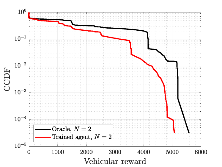
Figure 9: The CCDF of the vehicular reward achieved by trained agents and oracle for $N=2$.

Finally, and in order to assess the quality of the learned cooperative perception policy, we consider a network of only $N=2$ vehicles, with a maximum quadtree resolution level $L=2$. We compare our trained agent to an oracle, which knows exactly the RoI’s weights of each vehicle and selects the quadtree blocks that maximizes the vehicular satisfaction of both vehicles. Fig. 9 plots the CCDF of the achieved vehicular rewards of all the vehicles in both cases. It can be observed that the performance gap between the trained agent and the oracle is small, which proves the effectiveness of the proposed method in learning which quadtree blocks to transmit in order to enhance the cooperative perception.

VIII Conclusion

In this paper, we have studied the problem of associating vehicles, allocating RBs and selecting the contents of CPMs in order to maximize the vehicles’ satisfaction in terms of the received sensory information while considering the impact of the wireless communication. To solve this problem, we have resorted to the DRL techniques where two RL problems have been modeled. In order to overcome the huge action space inherent to the formulation of our RL problems, we applied the dueling and branching concepts. Moreover, we have proposed a federated RL approach to enhance and accelerate the training process of the vehicles. Simulation results show that policies achieving higher vehicular satisfaction could be learned at both the RSU and vehicular sides leading to a higher vehicular satisfaction.

References

- [1] M. K. Abdel-Aziz, S. Samarakoon, C. Perfecto, and M. Bennis, “Cooperative perception in vehicular networks using multi-agent reinforcement learning,” in Proc. of 54th Asilomar Conference on Signals, Systems, and Computers, Pacific Grove, CA, USA, Nov. 2020.
- [2] M. K. Abdel-Aziz, C. Perfecto, S. Samarakoon, and M. Bennis, “V2V cooperative sensing using reinforcement learning with action branching,” in Proc. of IEEE International Conference on Communications (ICC), Mobile and Wireless Networks Symposium, Montreal, Canada, Jun. 2021.
- [3] A. Ferdowsi, U. Challita, and W. Saad, “Deep learning for reliable mobile edge analytics in intelligent transportation systems: An overview,” IEEE Vehicular Technology Magazine, vol. 14, no. 1, pp. 62–70, Mar. 2019.
- [4] J. Park, S. Samarakoon, H. Shiri, M. K. Abdel-Aziz, T. Nishio, A. Elgabli, and M. Bennis, “Extreme urllc: Vision, challenges, and key enablers,” 2020. [Online]. Available: https://arxiv.org/pdf/2001.09683
- [5] ETSI TR 103 562 V2.1.1, “Intelligent Transport Systems (ITS); Vehicular Communications; Basic Set of Applications; Analysis of the Collective Perception Service (CPS); Release 2,” Dec. 2019.
- [6] M. Rondinone, T. Walter, R. Blokpoel, and J. Schindler, “V2X communications for infrastructure-assisted automated driving,” in Proc. of IEEE 19th International Symposium on A World of Wireless, Mobile and Multimedia Networks (WoWMoM), Chania, Greece, Jun. 2018, pp. 14–19.
- [7] S. D. Pendleton, H. Andersen, X. Du, X. Shen, M. Meghjani, Y. H. Eng, D. Rus, and M. H. Ang, “Perception, planning, control, and coordination for autonomous vehicles,” Machines, vol. 5, no. 1, 2017. [Online]. Available: https://www.mdpi.com/2075-1702/5/1/6
- [8] Y. Wang, G. de Veciana, T. Shimizu, and H. Lu, “Performance and scaling of collaborative sensing and networking for automated driving applications,” in Proc. of IEEE International Conference on Communications Workshops, Kansas City, MO, USA, May 2018, pp. 1–6.
- [9] M. Shan, K. Narula, Y. F. Wong, S. Worrall, M. Khan, P. Alexander, and E. Nebot, “Demonstrations of cooperative perception: Safety and robustness in connected and automated vehicle operations,” Sensors, vol. 21, no. 1, 2021. [Online]. Available: https://www.mdpi.com/1424-8220/21/1/200
- [10] 3GPP TR 22.886 V16.2.0 , “3rd Generation Partnership Project; Technical Specification Group Services and System Aspects; Study on enhancement of 3GPP Support for 5G V2X Services (Release 16),” Dec. 2018.
- [11] D. Garcia-Roger, E. E. González, D. Martín-Sacristán, and J. F. Monserrat, “V2X support in 3GPP specifications: From 4G to 5G and beyond,” IEEE Access, vol. 8, pp. 190 946–190 963, Oct. 2020.
- [12] G. Thandavarayan, M. Sepulcre, and J. Gozalvez, “Generation of cooperative perception messages for connected and automated vehicles,” IEEE Transactions on Vehicular Technology, pp. 1–1, Nov. 2020.
- [13] M. Gabb, H. Digel, T. Müller, and R.-W. Henn, “Infrastructure-supported perception and track-level fusion using edge computing,” in Proc. of IEEE Intelligent Vehicles Symposium (IV), Paris, France, Jun. 2019, pp. 1739–1745.
- [14] T. Zeng, O. Semiari, W. Saad, and M. Bennis, “Joint communication and control for wireless autonomous vehicular platoon systems,” IEEE Transactions on Communications, vol. 67, no. 11, pp. 7907–7922, Nov. 2019.
- [15] Q. Chen, S. Tang, Q. Yang, and S. Fu, “Cooper: Cooperative perception for connected autonomous vehicles based on 3D point clouds,” in Proc. of IEEE 39th International Conference on Distributed Computing Systems (ICDCS), Dallas, TX, USA, Jul. 2019, pp. 514–524.
- [16] E. Arnold, M. Dianati, R. de Temple, and S. Fallah, “Cooperative perception for 3d object detection in driving scenarios using infrastructure sensors,” IEEE Transactions on Intelligent Transportation Systems, pp. 1–13, 2020.
- [17] Q. Yang, S. Fu, H. Wang, and H. Fang, “Machine-learning-enabled cooperative perception for connected autonomous vehicles: Challenges and opportunities,” IEEE Network, vol. 35, no. 3, pp. 96–101, 2021.
- [18] C. Perfecto, J. Del Ser, M. Bennis, and M. N. Bilbao, “Beyond WYSIWYG: Sharing contextual sensing data through mmwave v2v communications,” in Proc. of European Conference on Networks and Communications (EuCNC), Oulu, Finland, Jun. 2017, pp. 1–6.
- [19] J. Choi, V. Va, N. Gonzalez-Prelcic, R. Daniels, C. R. Bhat, and R. W. Heath, “Millimeter-wave vehicular communication to support massive automotive sensing,” IEEE Communications Magazine, vol. 54, no. 12, pp. 160–167, Dec. 2016.
- [20] H. Samet, “The quadtree and related hierarchical data structures,” ACM Comput. Surv., vol. 16, no. 2, pp. 187–260, Jun. 1984. [Online]. Available: https://doi.org/10.1145/356924.356930
- [21] S. Kumar, L. Shi, N. Ahmed, S. Gil, D. Katabi, and D. Rus, “Carspeak: A content-centric network for autonomous driving,” SIGCOMM Comput. Commun. Rev., vol. 42, no. 4, pp. 259–270, Aug. 2012. [Online]. Available: https://doi.org/10.1145/2377677.2377724
- [22] P. Li, T. Zhang, C. Huang, X. Chen, and B. Fu, “RSU-assisted geocast in vehicular ad hoc networks,” IEEE Wireless Communications, vol. 24, no. 1, pp. 53–59, Feb. 2017.
- [23] Q. Delooz and A. Festag, “Network load adaptation for collective perception in V2X communications,” in Proc. of IEEE International Conference on Connected Vehicles and Expo (ICCVE), Graz, Austria, Nov. 2019, pp. 1–6.
- [24] S. Aoki, T. Higuchi, and O. Altintas, “Cooperative perception with deep reinforcement learning for connected vehicles,” 2020. [Online]. Available: https://arxiv.org/pdf/2004.10927
- [25] N. Zhao, Y. Liang, D. Niyato, Y. Pei, M. Wu, and Y. Jiang, “Deep reinforcement learning for user association and resource allocation in heterogeneous cellular networks,” IEEE Transactions on Wireless Communications, vol. 18, no. 11, pp. 5141–5152, Aug. 2019.
- [26] M. A. Abd-Elmagid, A. Ferdowsi, H. S. Dhillon, and W. Saad, “Deep reinforcement learning for minimizing age-of-information in UAV-assisted networks,” in Proc. of IEEE Global Communications Conference (GLOBECOM), Waikoloa, HI, USA, Dec. 2019, pp. 1–6.
- [27] X. Chen, C. Wu, T. Chen, H. Zhang, Z. Liu, Y. Zhang, and M. Bennis, “Age of information aware radio resource management in vehicular networks: A proactive deep reinforcement learning perspective,” IEEE Transactions on Wireless Communications, vol. 19, no. 4, pp. 2268–2281, Jan. 2020.
- [28] H. Ye, G. Y. Li, and B. F. Juang, “Deep reinforcement learning based resource allocation for V2V communications,” IEEE Transactions on Vehicular Technology, vol. 68, no. 4, pp. 3163–3173, Feb. 2019.
- [29] V. Mnih, K. Kavukcuoglu, D. Silver, A. A. Rusu, J. Veness, M. G. Bellemare, A. Graves, M. Riedmiller, A. K. Fidjeland, G. Ostrovski, S. Petersen, C. Beattie, A. Sadik, I. Antonoglou, H. King, D. Kumaran, D. Wierstra, S. Legg, and D. Hassabis, “Human-level control through deep reinforcement learning,” Nature, vol. 518, no. 7540, pp. 529–533, Feb 2015.
- [30] C. Nadiger, A. Kumar, and S. Abdelhak, “Federated reinforcement learning for fast personalization,” in 2019 IEEE Second International Conference on Artificial Intelligence and Knowledge Engineering (AIKE), Sardinia, Italy, Aug. 2019, pp. 123–127.
- [31] P. Kairouz, H. B. McMahan, B. Avent et al., “Advances and open problems in federated learning,” CoRR, vol. abs/1912.04977, 2019. [Online]. Available: https://arxiv.org/pdf/1912.04977
- [32] J. Park, S. Samarakoon, M. Bennis, and M. Debbah, “Wireless network intelligence at the edge,” Proceedings of the IEEE, vol. 107, no. 11, pp. 2204–2239, Oct. 2019.
- [33] A. Tavakoli, F. Pardo, and P. Kormushev, “Action branching architectures for deep reinforcement learning,” CoRR, vol. abs/1711.08946, 2017. [Online]. Available: http://arxiv.org/abs/1711.08946
- [34] S. Kaul, M. Gruteser, V. Rai, and J. Kenney, “Minimizing age of information in vehicular networks,” in Proc. of 8th Annual IEEE Communications Society Conference on Sensor, Mesh and Ad Hoc Communications and Networks, Salt Lake City, UT, USA, Jun. 2011, pp. 350–358.
- [35] M. K. Abdel-Aziz, S. Samarakoon, C. Liu, M. Bennis, and W. Saad, “Optimized age of information tail for ultra-reliable low-latency communications in vehicular networks,” IEEE Transactions on Communications, vol. 68, no. 3, pp. 1911–1924, Mar. 2020.
- [36] T. Mangel, O. Klemp, and H. Hartenstein, “A validated 5.9 GHz non-line-of-sight path-loss and fading model for inter-vehicle communication,” in 2011 11th International Conference on ITS Telecommunications, St. Petersburg, Russia, Aug. 2011, pp. 75–80.
- [37] R. S. Sutton and A. G. Barto, Reinforcement learning: An introduction. MIT press, 1998.
- [38] J. N. Tsitsiklis and B. Van Roy, “Analysis of temporal-diffference learning with function approximation,” in Advances in Neural Information Processing Systems 9, M. C. Mozer, M. I. Jordan, and T. Petsche, Eds. MIT Press, 1997, pp. 1075–1081. [Online]. Available: http://papers.nips.cc/paper/1269-analysis-of-temporal-diffference-learning-with-function-approximation.pdf
- [39] T. P. Lillicrap, J. J. Hunt, A. Pritzel, N. Heess, T. Erez, Y. Tassa, D. Silver, and D. Wierstra, “Continuous control with deep reinforcement learning,” 2015. [Online]. Available: https://arxiv.org/pdf/1509.02971
- [40] B. McMahan, E. Moore, D. Ramage, S. Hampson, and B. A. y Arcas, “Communication-efficient learning of deep networks from decentralized data,” ser. Proceedings of Machine Learning Research, A. Singh and J. Zhu, Eds., vol. 54. Fort Lauderdale, FL, USA: PMLR, 20–22 Apr 2017, pp. 1273–1282. [Online]. Available: http://proceedings.mlr.press/v54/mcmahan17a.html
- [41] S. Samarakoon, M. Bennis, W. Saad, and M. Debbah, “Distributed federated learning for ultra-reliable low-latency vehicular communications,” IEEE Transactions on Communications, vol. 68, no. 2, pp. 1146–1159, Nov. 2020.
- [42] P. A. Lopez and M. Behrisch and L. Bieker-Walz and J. Erdmann and Y. Flötteröd and R. Hilbrich and L. Lücken and J. Rummel and P. Wagner and E. Wiessner, “Microscopic traffic simulation using sumo,” in Proc. of 21st International Conference on Intelligent Transportation Systems (ITSC), Maui, HI, USA, Nov. 2018, pp. 2575–2582.