An Asynchronous Maximum Independent Set Algorithm by Myopic Luminous Robots on Grids

Abstract

We consider the problem of constructing a maximum independent set with mobile myopic luminous robots on a grid network whose size is finite but unknown to the robots. In this setting, the robots enter the grid network one-by-one from a corner of the grid, and they eventually have to be disseminated on the grid nodes so that the occupied positions form a maximum independent set of the network. We assume that robots are asynchronous, anonymous, silent, and they execute the same distributed algorithm. In this paper, we propose two algorithms: The first one assumes the number of light colors of each robot is three and the visible range is two, but uses additional strong assumptions of port-numbering for each node. To delete this assumption, the second one assumes the number of light colors of each robot is seven and the visible range is three. In both algorithms, the number of movements is $O(n(L+l))$ steps where $n$ is the number of nodes and $L$ and $l$ are the grid dimensions.

1 Introduction

Swarm robotics envisions groups of mobile robots self-organizing and cooperating toward the resolution of common objectives, such as patrolling, exploring and mapping disaster areas, constructing ad hoc mobile communication infrastructures to enable communication with rescue teams, etc. Our focus in this paper is the autonomous deployment of mobile robots in an unknown size rectangular area, e.g. for the purpose of establishing a communication infrastructure (if robots carry antennas) or a surveillance device (if robots carry intrusion sensors). When considering the rectangular area as a discrete structure (i.e., a graph, that depends on the antenna/sensor range: two nodes in the graph are adjacent if and only if they are within the range of the antenna/sensor), one can consider several placement strategies. Given that every location in the area must be covered by an antenna/sensor, there are two competing metrics:

1. The number of deployed robots: The cost of the deployment obviously depends linearly from the number of robots deployed.

2. The resilience of the infrastructure in the case robots fail unpredictably: This amounts to the number of locations that are left uncovered when a robot (or a set of robots) ceases to perform its algorithm.

Assuming full coverage is necessary, two extreme placement strategies are possible: A complete filling of each location by a robot enables maximum resilience (uncovering one location, say $C$ in Fig. 1(d), requires to disable five robots, at positions $A$, $B$, $C$, $D$ and $E$ in Fig. 1(d)) but also requires deploying one robot per location (so, the cost is highest), while a minimum dominating set strategy yields minimum cost, but poor resilience (disabling a single robot, say at $C$ in Fig. 1(c), uncovers five locations, $A$, $B$, $C$, $D$, and $E$ in Fig. 1(c)). Maximal and maximum independent set placements are somewhat more balanced, despite the fact that any robot failure will uncover its location: a maximal independent set may use as little as one-third of the robots required for a complete filling, while retaining decent resilience (e.g. in Fig. 1(a), at least two robots failures $C$ and $D$ are required to disconnect locations $A$ and $B$ beyond those initially hosting a robot); finally, a maximum independent set placement policy yields a resilience that is close to optimal (e.g. four robot failures, $A$, $B$, $C$, and $D$ disconnect only one additional location, $E$ in Fig. 1(b)) while using half of the robots required for a complete filling. In this paper, we concentrate on placing the robots according to a maximum independent set organization.

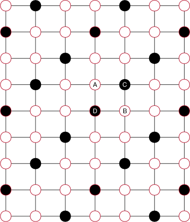
(a) Maximal Independent Set Placement

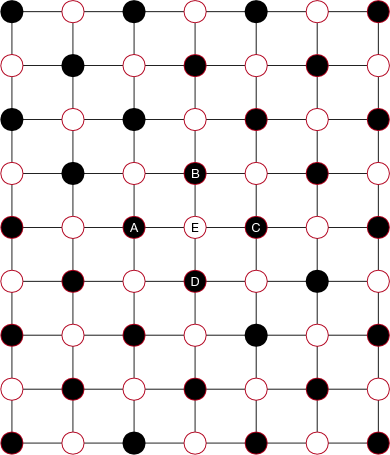
(b) Maximum Independent Set Placement

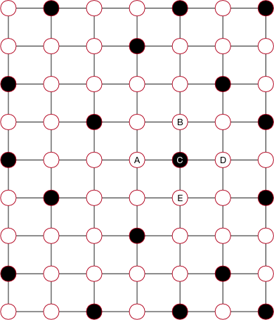
(c) Minimum Dominating Set Placement

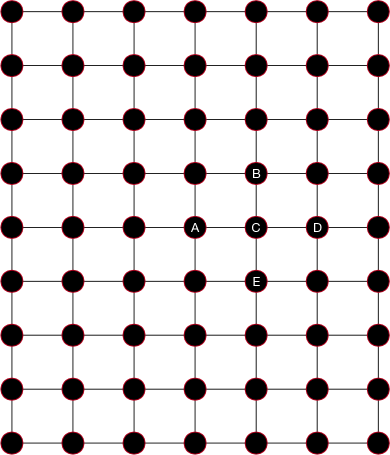
(d) Fill Placement

Figure 1: Possible mobile robot placements on a $7\times 9$ grid.

Related Works.

The seminal paper for studying robotic swarms from a distributed computing perspective is due to Suzuki and Yamashita [32]. In the initial model, robots are represented as dimensionless points evolving in a bidimensional Euclidean space, and operate in Look-Compute-Move cycles. In each cycle, a robot “Looks” at its surroundings and obtains (in its own coordinate system) a snapshot containing some information about the locations of all robots. Based on this visual information, the robot “Computes” a destination location (still in its own coordinate system), and then “Moves” towards the computed location. When the robots are oblivious, the computed destination in each cycle only depends on the snapshot obtained in the current cycle (and not on the past history of actions). Then, an execution of a distributed algorithm by a robotic swarm consists in having every robot repeatedly execute its LCM cycle. Although this mathematical model is perfectly precise, it allows a great number of variants (developed over a period of 20 years by different research teams [19]), according to various dimensions, namely: sensors, memory, actuators, synchronization, and faults.

Although the seminal paper [32] focused on continuous spaces, many recent papers [19] consider robots evolving on a discrete graph (that is, robots are located on a discrete set of locations, the nodes of the graph, and may move from one location to the next if an edge exists between the two locations), as it was recently observed that discrete observations model better actual sensing devices [2]. For the particular topology we consider, the grid, many problems were previously investigated, e.g., exploration  [14, 15], perpetual exploration [4], scattering [3], dispersion [28], gathering [11], mutual visibility [1], pattern formation [5], and convex hull formation [21]. Similarly, the initial model considers unlimited visibility range, but actual sensors have a limited range, which makes solutions that only assume limited visibility more practical. When the evolving space is discrete, robots that can only see at a constant (in the locations graph) are called myopic. Myopic robots have successfully solved ring exploration [13], gathering in bipartite graphs [20], and gathering in ring networks [26]. Finally, another characteristic of the initial model, obliviousness, was recently dropped out in favor of a more realistic setting: luminous robots. Oblivious robots were not able to remember past actions (each new Look-Compute-Move cycle reset the local memory of the robot), while luminous robots are able to remember and communicate a finite value between two consecutive LCM cycles, using a visible light that is maintained by the robot. The number of values a robot is able to remember is tantamount to the number of different colors its light is able to show. Luminous robots were used to circumvent classical impossibility results in the oblivious model, mainly for gathering [12, 33, 22]. In this paper, we consider the particular combination of myopic and luminous robot model, that was previously used for ring exploration [30, 29], infinite grid exploration [6], and gathering on rings [27].

The maximum independent set placement we consider in this paper is related to the benchmarking problem of geometric pattern formation initially proposed by Suzuki and Yamashita [32]. A key difference is that the target pattern is usually given explicitly to all robots (see the recent survey by Yamauchi [34]), while the maximum independent set pattern we target is only given as a constraint (as the dimensions of the grid are unknown to the robots, the exact pattern cannot be given to the robots). Unconstrained placement of robots is also known as scattering (in a continuous bidimensional Euclidean space [16, 9, 7], robots simply have to eventually occupy distinct positions). Evenly spreading robots in a unidimensional Euclidean space was previously investigated by Cohen and Peleg [10] and by Flocchini [17] and Flocchini et al. [18]. The bidimensional case was tackled mostly by means of simulation by Cohen and Peleg [10] and by Casteigts et al. [8]. Most related to our setting is the barrier coverage problem investigated by Hesari et al. [23]: robots have to move on a continuous line so that each portion of the line is covered by robot sensors (whose range is a fixed value) despite the robots having limited vision (whose range is twice the range of the sensor). A key difference besides the robots evolving space (continuous segment versus discrete grid) with our approach is that they consider oblivious robots and a common orientation, while we assume luminous robots and no orientation. Another closely related problem was studied by Barrière et al. [3]: uniform scattering on square grids. For uniform scattering to be solved, robots, initially at random positions, must reach a configuration where they are evenly spaced on a grid. Similarly to Hesari et al. [23], Barrière et al. [3] assume a common orientation (on both axes), that the size of the grid is $(k\times d+1)\times(k\times d+1)$, where $k\geq 2$, $d\geq 2$, the number of robots is $(k+1)^{2}$, and that each robot knows $k$ and $d$. They also assume that each robot has internal lights with six colors and that their visible radius is $2d$. Under the same assumptions as Barrière et al. [3], Poudel et al. [31] proposed an algorithm needing $O(1)$ bit memory per robot, assuming a visibility radius of $2\max\{d,k\}$. By contrast, we don’t assume a common orientation, we use seven or three full lights colors, and the size of the grid is arbitrary and unknown. Finally, the placement method we describe as the fill placement (see Fig. 1(d)) was investigated by Hsiang et al. [25], and by Hideg et al. [24].

Our contribution.

We propose the first two solutions to the maximum independent set placement of mobile myopic luminous robots on a grid of unknown size. Robots enter at a corner of the grid, and do not share a common orientation nor chirality. In the first algorithm, each robot light can take $3$ different colors, and the visibility range of each robot is two. Similarly to previous work [24], the first algorithm assumes ”local” port numbers are available at each node, so that each robot can recognize its previous node. The second algorithm gets rid of the port number assumption, and executes in a completely anonymous graph. It turns out that weakening this assumption has a cost on the number of colors ($7$ instead of $3$) and on the visibility radius ($3$ instead of $2$). In both cases, the placement process takes $O(n(L+l))$ steps of computation, where $n$ is the number of nodes and $L$ and $l$ are the grid dimensions.

As pointed out in the above, a maximum independent set placement yields good resilience in case of robot failures for the purpose of the target application, yet makes use of half of the robots needed for a complete filling of the grid.

2 Model

We consider an anonymous, undirected connected network $G^{\prime}=(V,E)$, where $V$ is a finite set of $n$ nodes $v_{1},v_{2},\cdots v_{n}$, and a specific node $v^{\prime}$ (discussed below), and $E$ is a finite set of edges. We assume that the induced subgraph $G$ of $G^{\prime}$ derived from the nodes except $v^{\prime}$ is a $(l,L)$-grid, where $l\geq 3$ and $L\geq 3$ are two positive integers such that $l\times L=n$. Then, $G$ satisfies the following conditions: $\forall x\in[1..n],(x\bmod l)\neq 0\Rightarrow\{v_{x},v_{x+1}\}\in E$, and $\forall y\in[1..l\times(L-1)],\{v_{y},v_{y+l}\}\in E$. We assume that these sizes $l$, $L$ and $n$ are unknown to the robots. Let $\delta(v)$ be the degree of node $v$ in $G^{\prime}$.

The specific node $v^{\prime}$ is called a Door node. Each robot enters the grid $G$ one-by-one through the Door node. We assume that $\delta(v^{\prime})=1$, and the Door node is connected to a corner node of the grid (the particular corner $v^{\prime}$ is connected to is decided by an adversary). We refer to this corner as the Door corner. A robot at the Door node has to disperse through the grid while avoiding collisions. That is, two or more robots cannot occupy the same node. When the Door node becomes empty, a new robot can be placed there immediately. We use ${\it Enter\_Grid}(r_{i})$ to denote an operation that makes robot $r_{i}$ move from the Door node to the Door corner, and ${\it Move}(r_{i})$ to denote an operation that makes $r_{i}$ move to an adjacent node in its direction. We assume that each robot has no orientation, i.e., each robot does not know axes $x$ and $y$ of the grid in the above definition.

The distance between two nodes $v$ and $u$ is the number of edges in a shortest path connecting them. The distance between two robots $r_{1}$ and $r_{2}$ is the distance between two nodes occupied by $r_{1}$ and $r_{2}$, respectively. Two robots or two nodes are adjacent if the distance between them is one.

We assume that robots have limited visibility: an observing robot $r_{i}$ at node $u$ can only sense the robots that occupy nodes within a certain distance, denoted by $\phi$, from $u$. When we assume $\phi=2$ (resp. $\phi=3$), because we assume the network is a grid, the view of a robot is like Fig. 2(a) (resp. 2(b)) for a robot not on a border nor a corner node. In each of these figures, the view is from a robot on the center node.

(a) $\phi=2$

(b) $\phi=3$

Figure 2: View of a robot.

For each robot $r_{i}$, we use ${\it view}(r_{i})$ to denote the view of $r_{i}$. Then, we call each robot $r_{j}$ in ${\it view}(r_{i})$ a neighboring robot of $r_{i}$.

Each robot $r_{i}$ maintains a variable $c(r_{i})$ called light, which spans a finite set of states called colors. A light is persistent from one computational cycle to the next: the color is not automatically reset at the end of the cycle (see below how cycles drive the life of robots). Robot $r_{i}$ knows its own current color of light and can detect colors of lights of other robots in the visibility range. Robots are unable to communicate with each other explicitly (e.g., by sending messages), however, they can observe their environment, including the positions and colors of other robots, in their visibility range.

Each robot $r_{i}$ executes Look-Compute-Move cycles infinitely many times: (i) first, $r_{i}$ takes a snapshot of the environment and obtains an ego-centered view of the current configuration (Look phase), (ii) according to its view, $r_{i}$ decides to move or to stay idle and possibly changes its light color (Compute phase), (iii) if $r_{i}$ decided to move, it moves to one of its adjacent nodes depending on the choice made in the Compute phase (Move phase). At each time instant $t$, a subset of robots is activated by an entity known as the scheduler. This scheduler is assumed to be fair, i.e., all robots are activated infinitely many times in any infinite execution. In this paper, we consider the most general asynchronous model: the time between Look, Compute, and Move phases is finite but unbounded. We assume however that the move operation is atomic, that is, when a robot takes a snapshot, it sees robots’ colors on nodes and not on edges. Since the scheduler is allowed to interleave the different phases between robots, some robots may decide to move according to a view that is different from the current configuration. Indeed, during the Compute phase, other robots may move. We call a view that is different from the current configuration an outdated view, and a robot with an outdated view an outdated robot.

In this paper, the set of robots that enter the grid $G$ from a Door node constructs a maximum independent set of $G$.

Definition 1

An independent set $I$ of $G$ is a subset of $V\setminus\{v^{\prime}\}$ such that no two nodes in $I$ are adjacent on $G$. A maximum independent set is an independent set containing the largest possible number of nodes for $G$.

3 Proposed Algorithms

In this section, we present two algorithms to construct a maximum independent set when the Door node is connected to a corner node. The first algorithm makes the assumption that outgoing edges are labeled “locally” (that is, the labels may be inconsistent for the two adjacent nodes of the edge, however, a node must assign distinct labels to different outgoing edges), and assumes that each robot is endowed with a light enabling $3$ colors and has visibility radius $2$. To remove the edge labeling assumption, the second algorithm makes use of more colors (7 colors are needed) and a larger visibility radius (i.e., $3$). As a result, it operates in the “vanilla” Look-Compute-Move model (no labeling of nodes or edges, etc.). In both algorithms, we assume no agreement on the grid axes or directions.

3.1 Algorithm with 3 colors lights, $\phi=2$, and port numbering

First, we propose an algorithm that assumes three light colors are available (and referred to as $F$, $p_{1}$, and $p_{2}$), and that $\phi=2$. The color $F$ means that the robot finished the execution of the algorithm, and stops its execution. Colors $p_{1}$ and $p_{2}$ are used when the robot still did not finish its execution. We say that if the light color of a robot $r_{i}$ is $F$, then $r_{i}$ is Finished. Initially, the color of the light $c(r_{i})$ for each robot $r_{i}$ is $p_{1}$.

For this algorithm, we add the following assumptions to the model in Section 2:

• For each node of the grid, adjacent nodes (except the Door node) are arranged in a fixed order, and this order is only visible for robots on the node as port numbers. The order does not change during the execution.

• Each robot can recognize the node it came from when at its current node.

These assumptions are those considered in related work for the filling problem [24]. Note that, the latter assumption can be implemented using four additional colors to remember the port number of the previous node.

The strategy of the routing to construct a maximum independent set is as Fig. 3. In this figure, the thick white circle represents a Finished robot, and the diagonal (resp. horizontal) striped circle represents a robot with $p_{1}$ (resp. $p_{2}$). First, each robot $r_{i}$ starts with $c(r_{i})=p_{1}$ from the Door node (Fig. 3(a)). On the Door corner, each robot chooses an adjacent node according to the edge with the maximal port number. Each robot moves on the first border to keep the distance from its predecessor two or more hops. Each robot arrives at the first corner, then changes $c(r_{i})$ to $p_{2}$. After that, the first robot $r_{1}$ goes through the second border, eventually arrives at the second corner (Fig. 3(b)), and changes $c(r_{1})$ to $F$. We call this second corner the diagonal corner. The successor $r_{i}$ follows its predecessor $r_{j}$ while striving to keep a distance of at least two. If $r_{i}$ has $c(r_{i})=p_{2}$, and $r_{j}$ is Finished two hops away, then $r_{i}$ changes $c(r_{i})$ to $F$ (Fig. 3(c)). If $r_{i}$ with $c(r_{i})=p_{1}$ observes that $r_{j}$ is Finished two hops away, $r_{i}$ changes $c(r_{i})$ to $p_{2}$ and makes the next line (Fig. 3(d)). By repeating such elementary steps, eventually, a maximum independent set can be constructed (Fig. 3(f)). Because each robot can recognize its previous node by the assumption, it can recognize its predecessor and its successor if there are two neighboring non-Finished robots.

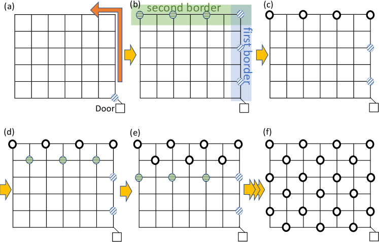
Figure 3: Strategy of the maximum independent set placement from a Door node on a corner.

The algorithm description is in Algorithm 1. The number of each rule represents its priority, a smaller number denoting a higher priority. In this algorithm, we use the definitions of view types in Fig. 5–9. In these figures, each view ${\it view}(r_{i})$ is from robot $r_{i}$ represented by the center filled circle. The dotted circle without frame border represents the previous node wherefrom $r_{i}$ moved to the current node. If ${\it view}(r_{i})$ is a view with an arrow from $r_{i}$ not on the Door node (like OnCP1 in ${\cal C}$ (Fig. 6)), the arrow represents the direction of ${\it Move}(r_{i})$ operation. If $r_{i}$ is on the Door node (like Door1 in ${\cal D}$ (Fig. 5)), the arrow represents the operation ${\it Enter\_Grid}(r_{i})$. If the previous node is not the Door node, the circle with diagonal stripes or horizontal stripes (which is adjacent to the previous node) represents the node where $r_{i}$’s successor robot may be hosted. So, such a node may: (i) host the successor of $r_{i}$, (ii) be empty, or (iii) do not exist. If the successor robot is on the diagonal (resp. horizontal) striped node, it has $p_{1}$ (resp. $p_{1}$ or $p_{2}$). The diagonal striped node can be the Door node under the grid size hypothesis, i.e., the diagonal striped node in P1Stop can be the Door node but in OnCP1F cannot be the Door node due the grid size hypothesis. If the previous node is the Door node, the successor robot can be the previous node by assumption. The thick white circle represents a Finished robot that must be on the node. The circle with vertical stripes represents either a node hosting a Finished robot, or no node. A node with a dashed white square represents an empty node, if the node exists on the grid. All other empty nodes must exist on the grid and host no robot. In our classification, each type of views may include several possible views. For example, in P1Stop (Fig. 5), the upper adjacent empty node may be a corner, then the top node with vertical stripes does not exist. Thus, in the type P1Stop, there are five possible views, depending on whether the top node exists or not, the bottom node exists or not, and whether the successor is in the view or not. Note that all combinations are not feasible, since e.g. if the bottom node does not exist, then the previous node is the Door node, and the successor is on the Door node, which in turn implies that the top Finished robot must exist (due to the grid size hypothesis).

Colors  $F$, $p_{1}$, $p_{2}$
Iinitialization  $c(r_{i})=p_{1}$
Rules on node $v$ of robot $r_{i}$
0: $c(r_{i})=p_{1}\land{\it view}(r_{i})\in{\cal D}$ $\rightarrow$ ${\it Enter\_Grid}(r_{i})$;
1: $c(r_{i})=p_{1}\land{\it view}(r_{i})\in{\cal F}_{1}$ $\rightarrow$ $c(r_{i}):=F$;
2: $c(r_{i})=p_{1}\land{\it view}(r_{i})\in{\cal C}$ $\rightarrow$ $c(r_{i}):=p_{2}$; ${\it Move}(r_{i})$;
3: $c(r_{i})=p_{1}\land{\it view}(r_{i})\in{\cal M}_{1}$ $\rightarrow$ ${\it Move}(r_{i})$;
4: $c(r_{i})=p_{2}\land{\it view}(r_{i})\in{\cal F}_{2}$ $\rightarrow$ $c(r_{i}):=F$;
5: $c(r_{i})=p_{2}\land{\it view}(r_{i})\in{\cal M}_{2}$ $\rightarrow$ ${\it Move}(r_{i})$.

Algorithm 1 Algorithm for a maximum independent set placement with 3 colors light.

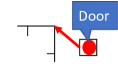
(a) Door1

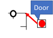
(b) Door2

Figure 4: Definition of views in ${\cal D}$ while $p_{1}$.

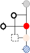
(a) P1Stop

(b) OnCP1F

Figure 5: Definition of views in ${\cal F}_{1}$ while $p_{1}$.

(a) OnCP1

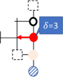
(b) ColP1A

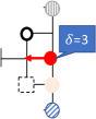
(c) ColP1B

Figure 6: Definition of views in ${\cal C}$ while $p_{1}$.

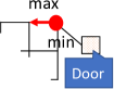
(a) StartP1

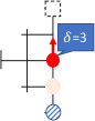
(b) MovP1

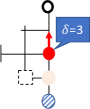
(c) GoCo

Figure 7: Definition of views in ${\cal M}_{1}$ while $p_{1}$.

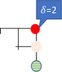
(a) OnCP2

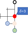
(b) P2Stop

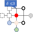
(c) P2StopA

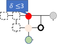
(d) P2StopB

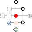
(e) P2StopC

Figure 8: Definition of views in ${\cal F}_{2}$ while $p_{2}$.

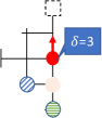
(a) MovP2

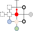
(b) MovP2A

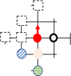
(c) MovP2B

Figure 9: Definition of views in ${\cal M}_{2}$ while $p_{2}$.

3.1.1 Proof of Correctness

Without loss of generality, let $L$ be the size of the border that is connected to the Door corner by an edge with a maximal port number among two edges of the Door corner. Let $l$ be the other size of the border. We call the $L$-size border connected to the Door corner “the first border”, and the $l$-size border not-connected to the Door corner “the second border”, like Fig. 3(b). Additionally, we call the second border 0-line, and count the lines in the following way: the line that is adjacent and parallel to 0-line is 1-line, and the border that is connected to the Door corner but not the first border is $(L-1)$-line.

First, we show that robots cannot collide.

Lemma 1

Robots cannot collide when executing Algorithm 1.

Proof

If there exists an outdated robot $r_{o}$ that is to move using its outdated view, the outdated view is one of the types in ${\cal D}$, ${\cal C}$, ${\cal M}_{1}$, or ${\cal M}_{2}$ by the definition of the algorithm. Thus, if a collision with $r_{o}$ occurs, then $r_{o}$’s view is one of the types in ${\cal D}$, ${\cal C}$, ${\cal M}_{1}$, or ${\cal M}_{2}$. In that case, because a Finished robot does not move forever, a non-Finished robot in $r_{o}$’s view may have moved, or other non-Finished robot came into the visible region of $r_{o}$.

On the Door corner, if a robot $r_{i}$ cannot see other robots, then its view is StartP1 in ${\cal M}_{1}$. Then, because $r_{i}$ has $c(r_{i})=p_{1}$ initially, its view becomes MovP1 in ${\cal M}_{1}$. By the definition of MovP1, $r_{i}$ moves only on the first border according to the degree of nodes until it arrives at the end of the first border, or it can see Finished robots. Then, the first border is one-way because each robot can recognize its previous node. Additionally, if $r_{i}$ can see other non-Finished robots than its successor, then $r_{i}$ cannot move because there is no such rule. That is, $r_{i}$ keeps the distance from its predecessor (if it exists) two or more hops on the first border. Thus, on the first border (while $c(r_{i})=p_{1}$), if $r_{i}$ has an outdated view in ${\cal D}$, ${\cal C}$, or ${\cal M}_{1}$, the current configuration can be the same view type as its outdated view, because only $r_{i}$’s successor is allowed to move toward $r_{i}$. Thus, $r_{i}$ cannot collide with other robots while $c(r_{i})=p_{1}$.

Consider when $r_{i}$ arrives at the end of the first border, or can see Finished robots.

• If ${\it view}(r_{i})$ becomes P1Stop or OnCP1F in ${\cal F}_{1}$, then $r_{i}$ changes its color to $F$ by Rule 1.

• If ${\it view}(r_{i})$ becomes OnCP1 in ${\cal C}$, then $r_{i}$ changes its color to $p_{2}$, and moves to the second border by Rule 2. After that, ${\it view}(r_{i})$ becomes MovP2 in ${\cal M}_{2}$ until it arrives at the diagonal corner (i.e., OnCP2 in ${\cal F}_{2}$), or it can see Finished robots on the second border (i.e., P2Stop in ${\cal F}_{2}$). By the definition of MovP2, each robot moves on the second border according to the degree of nodes, and the second border is one-way. By the definition of the algorithm, there is no rule to make $r_{i}$ stray from the second border. Then, $r_{i}$ keeps the distance from its predecessor (if it exists) two or more hops on the second border.

• If ${\it view}(r_{i})$ becomes GoCo in ${\cal M}_{1}$, then $r_{i}$ moves to the adjacent node occupied by a Finished robot on the first border and ${\it view}(r_{i})$ becomes ColP1A in ${\cal C}$.

• If ${\it view}(r_{i})$ becomes ColP1A or ColP1B in ${\cal C}$, then $r_{i}$ changes its color to $p_{2}$, and moves to one of the lines. Without loss of generality, let the line be $m$-line where $m>0$. Then, robots on $(m-1)$-line are Finished and $(m+1)$-line is empty (if it exists on the grid) by the definition of ColP1A or ColP1B. Thus, after that, ${\it view}(r_{i})$ becomes MovP2A or MovP2B in ${\cal M}_{2}$ until it arrives at the end of $m$-line (i.e., P2StopA or P2StopB in ${\cal F}_{2}$), or it can see a Finished robot on $m$-line (i.e., P2StopC in ${\cal F}_{2}$). By the definition of the algorithm, there is no rule to make $r_{i}$ stray from $m$-line. By the definitions of MovP2A and MovP2B, $m$-line is also one-way, and $r_{i}$ keeps the distance from its predecessor (if it exists on the line) two or more hops.

In any case, on each line (while $c(r_{i})=p_{2}$), if $r_{i}$ has an outdated view in ${\cal C}$ or ${\cal M}_{2}$, then the current configuration is the same view type as its outdated view, because only $r_{i}$’s successor is allowed to move toward $r_{i}$. Thus, $r_{i}$ cannot collide with other robots while $c(r_{i})=p_{2}$.

Thus, the lemma holds. $\Box$

Next, we show that Algorithm 1 constructs a maximum independent set.

Lemma 2

The first robot $r_{1}$ moves to the diagonal corner, and $c(r_{1})$ becomes $F$ on the corner.

Proof

When the first robot $r_{1}$ is in the Door node, then its view is Door1 in ${\cal D}$. Thus, it moves to the Door corner by ${\it Enter\_Grid}(r_{1})$, and its view becomes StartP1 in ${\cal M}_{1}$. Then, $r_{1}$ moves to the adjacent node through the edge with the maximal port number by Rule 3. Then, because it is the first robot, its view becomes MovP1 in ${\cal M}_{1}$ and moves to the adjacent node on the first border by Rule 3.

By the proof of Lemma 1, the first border and second border are one-way, and any other robots cannot pass $r_{1}$ on these borders. Thus, ${\it view}(r_{1})$ remains MovP1, and $r_{1}$ moves on the first border according to the node degree. Therefore, $r_{1}$ arrives at the end of the first border eventually, and then ${\it view}(r_{1})$ becomes OnCP1 in ${\cal C}$. After that, by Rule 2, $r_{1}$ changes its color to $p_{2}$ and moves to the adjacent node on the second border. ${\it view}(r_{1})$ becomes MovP2 in ${\cal M}_{2}$, $r_{1}$ moves towards the next (diagonal) corner through the second border according to the node degree by Rule 5, eventually ${\it view}(r_{1})$ becomes OnCP2 in ${\cal F}_{2}$. By Rule 4, because $c(r_{1})=p_{2}$, $r_{1}$ changes its color to $F$ on the corner.

Thus, the lemma holds. $\Box$

Lemma 3

The first $\lceil l/2\rceil$ robots move to the second border, and their color becomes $F$. Additionally, nodes on the second border are occupied by a robot or empty alternately from the diagonal corner.

Proof

By Lemma 2, the first robot $r_{1}$ eventually becomes Finished on the diagonal corner.

First, we consider the second robot $r_{2}$, which follows $r_{1}$ in the case that $l>3$. By the assumption, $r_{2}$ appears to the Door node just after $r_{1}$ enters into the grid. Because $r_{1}$ does not become Finished before it arrives at the diagonal corner, $r_{2}$ can move from the Door node only when ${\it view}(r_{2})={\sf Door1}$ in ${\cal D}$ holds. After that, by the definition of the algorithm, $r_{2}$ moves in the same way as $r_{1}$, $c(r_{2})$ becomes $p_{2}$ on the end of the first border eventually and $r_{2}$ moves on the second border. Finally, $r_{2}$ can see $r_{1}$ on the diagonal corner two hops away. Then, there is no rule such that $r_{2}$ executes before $c(r_{1})$ becomes $F$. Because of Lemma 2, ${\it view}(r_{2})$ eventually becomes P2Stop in ${\cal F}_{2}$. Then, by Rule 4, $c(r_{2})$ becomes $F$.

In the case that $l=3$, when $r_{2}$ arrives at the end of the first border, ${\it view}(r_{2})$ becomes OnCP1F in ${\cal F}_{1}$ and $c(r_{2})$ becomes $F$ by Rule 1. Note that, in any case, the distance between $r_{1}$ and $r_{2}$ is two hops when they are Finished.

For the successors of $r_{2}$, we can discuss their movements in the same way as $r_{2}$. Thus, by the definitions of OnCP1F and P2Stop, the distance between a robot and its successor is two hops when they are Finished on the second border. Therefore, on the second border, beginning with the diagonal corner, every even node is occupied, and the number of robots is $\lceil l/2\rceil$. If $l$ is odd, when the $\lceil l/2\rceil$-th robot arrives at the end of the first border, its view becomes OnCP1F and it changes its color to $F$ by Rule 1. Otherwise, it changes its color to $p_{2}$ and moves to the second border.

Thus, the lemma holds. $\Box$

Lemma 4

From the $(\lceil l/2\rceil+1)$-th to the $l$-th robots, each robot moves to the $1$-line, and its color becomes $F$. Additionally, nodes on the $1$-line are empty or occupied by a robot alternately, beginning with an empty node.

Proof

By Lemma 3, $\lceil l/2\rceil$ robots on $0$-line eventually become Finished. Let $r_{i}$ be the $(\lceil l/2\rceil+1)$-th robot, $r_{j}$ be the $(\lceil l/2\rceil)$-th robot that is the predecessor of $r_{i}$. $r_{i}$ moves from the Door node in the same way as $r_{j}$ while $c(r_{i})=p_{1}$. Because robots on $0$-line become Finished eventually, one of the following two cases occurs: (1) if $l$ is odd, ${\it view}(r_{i})$ becomes GoCo in ${\cal M}_{1}$, because the end of the first border is occupied by $r_{j}$, or (2) if $l$ is even, ${\it view}(r_{i})$ becomes ColP1B in ${\cal C}$, because the end of the first border is empty but its adjacent node on the $0$-line is occupied by $r_{j}$.

In case (1), by Rule 3, $r_{i}$ moves to the node in front of the end of the first border, ${\it view}(r_{i})$ becomes ColP1A in ${\cal C}$. Then, by Rule 2, $c(r_{i})$ becomes $p_{2}$ and $r_{i}$ moves to $1$-line. After that, if $l=3$, ${\it view}(r_{i})$ becomes P2StopA in ${\cal F}_{2}$ and $r_{i}$ changes its color to $F$ by Rule 4. Otherwise, because $r_{i}$ can see Finished robots on $0$-line, ${\it view}(r_{i})$ becomes MovP2A in ${\cal M}_{2}$. Then, because the nodes on $0$-line are occupied alternately by Lemma 3, ${\it view}(r_{i})$ becomes MovP2B and MovP2A in ${\cal M}_{2}$ alternately by the execution of Rule 5. Thus, $r_{i}$ moves toward the other side border that is parallel to the first border by Rule 5, and ${\it view}(r_{i})$ eventually becomes P2StopA because the diagonal corner is occupied by a Finished robot (Lemma 2). Then, by Rule 4, $c(r_{i})$ eventually becomes $F$. Because $l$ is odd, $\lfloor l/2\rfloor-1$ successors of $r_{i}$ follow $r_{i}$, and eventually, their views become P2StopC in ${\cal F}_{2}$, and they change their colors to $F$ by Rule 4 on $1$-line.

In case (2), $r_{i}$ also changes its color to $p_{2}$, and moves to $1$-line by Rule 2. After that, because $r_{i}$ can see Finished robots on $0$-line, ${\it view}(r_{i})$ becomes MovP2B in ${\cal M}_{2}$. Then, in the same way as for case (1), $l/2-1$ robots including $r_{i}$ become Finished on $1$-line. After that, the view of the next robot $r_{l}$ ($l$-th robot) becomes P1Stop in ${\cal F}_{1}$ on the intersection between the first border and $1$-line, and $r_{l}$ becomes Finished by Rule 1.

Thus, the lemma holds. $\Box$

Lemma 5

The distance between any two robots on the grid is two hops after every robot becomes Finished.

Proof

By the definitions of ${\cal F}_{1}$ and ${\cal F}_{2}$, the distance between a robot $r_{i}$ and its predecessor is two hops after $r_{i}$ becomes Finished if the predecessor is on the same line as $r_{i}$. Thus, when the robots on $m$-line ($0<m<L-1$) become Finished, if there are two adjacent Finished robots, then there is a robot $r_{r}$ on $m$-line that cannot move from the node that is adjacent to a node occupied by a Finished robot on $(m-1)$-line. However, by the same argument as in Lemmas 3 and 4, if $m$ is odd (resp. even), the nodes on $m$-line are occupied alternately beginning with an empty node (resp. occupied node) because the nodes on $(m-1)$-line are also occupied alternately beginning with an occupied node (resp. empty node). Thus, before such $r_{r}$ becomes Finished, $r_{r}$ has a view of type MovP2B and can move by Rule 5, i.e., it cannot exist.

Now, to consider the end of the execution of the algorithm, we consider $(L-1)$-line when nodes on $(L-2)$-line are occupied by Finished robots. The $(L-1)$-line is a border connected to the Door node. Then, if both $l$ and $L$ are odd or both are even, the view from the Door node becomes Door1, otherwise Door2 (See Fig. 10).

• If the view from the Door node is Door1, the robot on the Door node moves to the Door corner by Rule 0. Then, the view from the Door corner is ColP1B in ${\cal C}$. By the above discussion, the view from the Door corner eventually becomes P1Stop in ${\cal F}_{1}$, thus the final robot on the Door corner becomes Finished by Rule 1. Then, any other robots cannot enter into the grid because there is no such rule.

• If the view from the Door node is Door2, the view from the Door corner is ColP1A in ${\cal C}$. Then, the empty node $v$ that is adjacent to the Door corner is eventually occupied by a Finished robot on $(L-1)$-line. After that, any other robots on the Door node cannot enter into the grid because there is no such rule.

Thus, the lemma holds. $\Box$

Lemma 6

Every robot on the grid is eventually Finished.

Proof

By the proofs of Lemmas 1-5, the transitions of the view type of each robot are shown as Fig. 11. Thus, the lemma holds. $\Box$

Theorem 3.1

Algorithm 1 constructs a maximum independent set of occupied locations on the grid.

Proof

By Lemma 5, distances between any two occupied nodes are two. On a grid, only checkers patterns satisfy this constraint. When at least one dimension of even, there are as many occupied locations as non-occupied locations, so any checkers pattern is a maximum independent set (see Fig. 10(a) and Fig. 10(b)). When both dimensions are odd, there may be either one more occupied locations than non-occupied locations, or the contrary (See Fig. 10(c)). The situation that corresponds to the maximum independent set is the one with occupied locations in the corners, which is what our algorithm constructs. Hence, the theorem holds. $\Box$

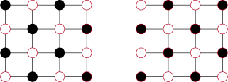
(a) even-even dimensions

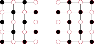
(b) even-odd dimensions

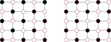
(c) odd-odd dimensions

Figure 10: Checkers patterns in grids.

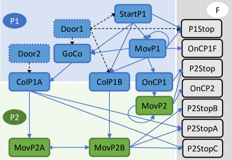
Figure 11: View type transitions of Algorithm 1. Each solid arrow (resp. dotted arrow) represents a transition by a Move (resp. Enter_Grid) operation.

Lemma 7

When a maximum independent set is constructed, $\lceil n/2\rceil$ robots are on the grid.

Proof

By the proofs of Lemmas 3–5, nodes on the even-numbers (resp. odd-numbers) lines are occupied by $\lceil l/2\rceil$ (resp. $\lfloor l/2\rfloor$) robots. Therefore, if $L$ is even, the number of robots in the maximum independent set is $lL/2$. If $L$ is odd, the number of robots in the maximum independent set is $l\lfloor L/2\rfloor+\lceil l/2\rceil$. Because $n=lL$, the lemma holds. $\Box$

To analyze the time complexity of the algorithm, we count the sum of individual executions of rules.

Theorem 3.2

The time complexity by Algorithm 1 is $O(n(L+l))$ steps.

Proof

The first robot moves $L+l-1$ steps and becomes Finished, thus it executes $L+l$ steps. The first robot moves the longest way. Therefore, by Lemma 7, the sum of the number of steps is $O(n(L+l))$. Thus, the theorem holds. $\Box$

3.2 Algorithm with 7 colors lights, and $\phi=3$

In this section, we relax both additional hypotheses made in Section 3.1. So, there is no local labeling of edges, and robots cannot recognize the node they came from when at a particular node. Instead, we assume $\phi=3$, and that seven light colors are available for each robot $r_{i}$, whose colors are named $F$, $p_{1}(k_{i})$, and $p_{2}(k_{i})$ ($k_{i}\in\{0,1,2\}$). The value of $k_{i}$ represents the order of the robot (the notion of order is explained in detail in the sequel). Initially, the color of light $c(r_{i})$ for each robot $r_{i}$ is $p_{1}(0)$, that is, $k_{i}=0$.

The strategy to construct a maximum independent set is the same as Algorithm 1. However, on the Door node, the first robot chooses an adjacent node on the grid arbitrarily (that is, the choice can be taken by an adversary), and the other robots just follow it.

The algorithm description is in Algorithm 2. In this algorithm, we use the definitions of view types in Fig. 13–18. Unlike Algorithm 1, we do not use dotted circles without frames, since the previous node can no longer be recognized by the robot. The circle with diagonal stripes or horizontal stripes represents $r_{i}$’s successor robot, which must be there (We explain later in the text how to recognize predecessor and successor). If the successor robot is on the diagonal (resp. horizontal) striped node, it has $p_{1}$ (resp. $p_{1}$ or $p_{2}$). While there are two types of successor in each view type of Fig. 17–18, exactly one must be present. The waffle circle represents $r_{i}$’s non-Finished predecessor robot. If the waffle circle is with a thick border, the predecessor must be there. Otherwise, it may be an empty node or non-existent node. For example, in the type Door2 (Fig. 13), when the predecessor has just become Finished on the upper node with the thick white circle, the waffle circle with the dotted border is actually an empty node. The square with a question mark represents any node in Door0 (Fig. 13).

By the strategy of the routing described above, each robot enters the grid one-by-one and walks in line on the grid. Therefore, each robot has a successor, and each robot except the first one has a predecessor. In this algorithm, each robot has a variable $k_{i}$ to distinguish them. On the Door node, each robot $r_{i}$ sets its $k_{i}$ (Door0 in Fig.13). If $r_{i}$ is the first robot, keeps $k_{i}=0$. Otherwise, if its predecessor robot $r_{j}$ on the Door corner has $p_{1}(k_{j})$, then $k_{i}$ is set to $(k_{j}+1)\mod 3$. The value of $k_{i}$ is kept in $c(r_{i})$ such that $p_{1}(k_{i})$ and $p_{2}(k_{i})$, and $k_{i}$ is not changed after that. On the Door corner, each robot $r_{j}$ waits for its successor $r_{i}$ on the Door node to set its value $k_{i}$ before $r_{j}$ moves (ColP1A1 and ColP1B1 in Fig. 15, and StartP10, StartP11, MovP13, MovP14 and GoCo1 in Fig. 16). By this mechanism, each robot $r_{i}$ recognizes that its neighboring non-Finished robot $r_{j}$ with smaller (resp. larger) $k_{j}$ value than $k_{i}$ is its predecessor (resp. successor). Let ${\it SetC}(r_{i})$ be the operation such that $c(r_{i}):=p_{1}((k_{j}+1)\mod 3)$, where $r_{j}$ is the robot on the Door corner and $c(r_{j})=p_{1}(k_{j})$.

Only the first robot selects its way arbitrarily from the Door corner (StartP10 in Fig. 16). After that, the other robot $r_{i}$ can move only when the distance from its predecessor is three (unless the predecessor becomes Finished) and the distance from its successor is two (unless $r_{i}$ is not on the Door corner). By this mechanism, $r_{i}$ can recognize which border is the first border chosen by the first robot on the Door corner.

Colors  $F$, $p_{1}(k_{i})$, $p_{2}(k_{i})$, where $k_{i}\in\{0,1,2\}$
Initialization  $c(r_{i})=p_{1}(0)$
Rules on node $v$ of robot $r_{i}$
0-1: $c(r_{i})=p_{1}(0)\land{\it view}(r_{i})={\sf Door0}$ $\rightarrow$ ${\it SetC}(r_{i})$;
0-2: $c(r_{i})=p_{1}(k_{i})\land{\it view}(r_{i})\in{\cal D}^{\prime}$ $\rightarrow$ ${\it Enter\_Grid}(r_{i})$;
1: $c(r_{i})=p_{1}(k_{i})\land{\it view}(r_{i})\in{\cal F}_{1}^{\prime}$ $\rightarrow$ $c(r_{i}):=F$;
2: $c(r_{i})=p_{1}(k_{i})\land{\it view}(r_{i})\in{\cal C}^{\prime}$ $\rightarrow$ $c(r_{i}):=p_{2}(k_{i})$; ${\it Move}(r_{i})$;
3: $c(r_{i})=p_{1}(k_{i})\land{\it view}(r_{i})\in{\cal M}_{1}^{\prime}$ $\rightarrow$ ${\it Move}(r_{i})$;
4: $c(r_{i})=p_{2}(k_{i})\land{\it view}(r_{i})\in{\cal F}_{2}^{\prime}$ $\rightarrow$ $c(r_{i}):=F$;
5: $c(r_{i})=p_{2}(k_{i})\land{\it view}(r_{i})\in{\cal M}_{2}^{\prime}$ $\rightarrow$ ${\it Move}(r_{i})$;

Algorithm 2 Algorithm for a maximum independent set placement with 7 colors light.

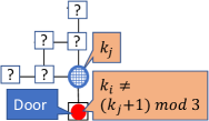
Figure 12: Door0.

(a) Door1

(b) Door2

(c) Door3

(d) Door4

Figure 13: Definition of Door0 and views in ${\cal D}^{\prime}$ while $p_{1}$.

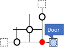
(a) P1Stop0

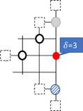
(b) P1Stop1

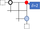
(c) OnCP1F

Figure 14: Definition of views in ${\cal F}_{1}^{\prime}$ while $p_{1}$.

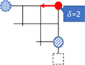
(a) OnCP1

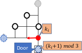
(b) ColP1A1

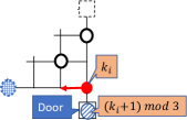
(c) ColP1B1

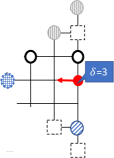
(d) ColP1A0

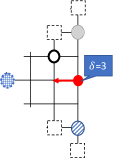
(e) ColP1B0

Figure 15: Definition of views in ${\cal C}^{\prime}$ while $p_{1}$.

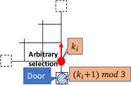
(a) StartP10

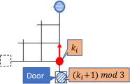
(b) StartP11

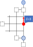
(c) MovP10

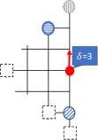
(d) MovP11

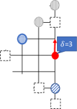
(e) MovP12

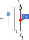
(f) GoCo0

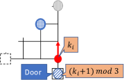
(g) MovP13

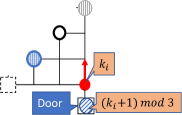
(h) MovP14

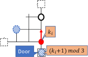
(i) GoCo1

Figure 16: Definition of views in ${\cal M}_{1}^{\prime}$ while $p_{1}$.

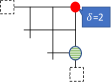
(a) OnCP2

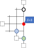
(b) P2Stop

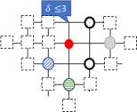
(c) P2StopA

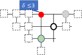
(d) P2StopB

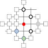
(e) P2StopC

Figure 17: Definition of views in ${\cal F}_{2}^{\prime}$ while $p_{2}$.

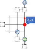
(a) MovP2

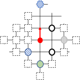
(b) MovP2A

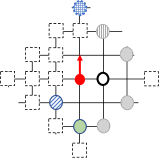
(c) MovP2B

Figure 18: Definition of views in ${\cal M}_{2}^{\prime}$ while $p_{2}$.

3.2.1 Proof of Correctness

Without loss of generality, let $L$ be the size of the border chosen by the first robot on the Door corner in StartP10 in ${\cal M}_{1}^{\prime}$. Let $l$ be the other size of the border. In the same way as Algorithm 1, we define “the first border”, “the second border”, and lines.

In the following, we first show that each robot can recognize its successor and robots cannot collide.

Lemma 8

Each non-Finished robot except the first robot can recognize its predecessor and successor if it keeps two neighboring non-Finished robots.

Proof

By the assumption, each robot $r_{i}$ initializes its $c(r_{i})$ to $p_{1}(0)$. The view of the first robot $r_{1}$ on the Door node is Door1 in ${\cal D}^{\prime}$, thus it moves to the Door corner with $c(r_{1})=p_{1}(0)$ by Rule 0-2. After that, by the assumption, its successor $r_{2}$ appears on the Door node with $c(r_{2})=p_{1}(0)$. Thus, $r_{1}$ cannot move until its view becomes StartP10 in ${\cal M}_{1}^{\prime}$, i.e., $r_{2}$ has $c(r_{2})=p_{1}((k_{1}+1)\mod 3))=p_{1}((0+1)\mod 3)=p_{1}(1)$. Thus, ${\it view}(r_{2})$ on the Door node becomes Door0 and $r_{2}$ sets $c(r_{2})$ to $p_{1}(1)$ by Rule 0-1. Then, ${\it view}(r_{1})$ becomes StartP10 in ${\cal M}_{1}^{\prime}$, $r_{1}$ selects the first border arbitrarily and moves on the border by Rule 3.

Consider a robot $r_{i}$ sets $c(r_{i})$ to $p_{1}(k_{i})$ on the Door node in Door0. Then, its predecessor $r_{h}$ on the Door corner has $c(k_{h})$ where $k_{i}=(k_{h}+1)\mod 3$ by the definition of ${\it SetC}(r_{i})$. After $r_{i}$ enters the grid, on the Door corner, it cannot move until its successor $r_{j}$ sets $c(r_{j})$ to $p_{1}(k_{j})$ where $k_{j}=(k_{i}+1)\mod 3$ by the definitions of StartP11, MovP13, MovP14, GoCo1 (in ${\cal M}_{1}^{\prime}$), ColP1A1 or ColP1B1 (in ${\cal C}^{\prime}$). Therefore, each robot $r_{i}$ on the grid has its order modulo 3 as its value $k_{i}$, and the value $k_{i}$ is not changed after that. Thus, if each robot keeps two neighboring non-Finished robots, it can recognize its neighboring non-Finished robot with smaller (resp. larger) $k$ value than its own as its predecessor (resp. successor), lemma holds. $\Box$

Lemma 9

While the light color is $p_{1}(k_{i})$, each robot $r_{i}$ can recognize its successor, and cannot collide.

Proof

If there exists an outdated robot $r_{o}$ that is to move according to its outdated view, the view type is in ${\cal D}^{\prime}$, ${\cal C}^{\prime}$, ${\cal M}_{1}^{\prime}$, and ${\cal M}_{2}^{\prime}$ by the definition of the algorithm. Thus, if a collision with $r_{o}$ occurs, then $r_{o}$’s view type is in ${\cal D}^{\prime}$, ${\cal C}^{\prime}$, ${\cal M}_{1}^{\prime}$, and ${\cal M}_{2}^{\prime}$. In that case, because a Finished robot does not move forever, it could be that a non-Finished robot in $r_{o}$’s view moved, or that another non-Finished robot came into the visible region of $r_{o}$.

The first robot $r_{1}$ keeps its color $c(r_{1})=p_{1}(0)$. On the Door node, the view of $r_{1}$ becomes Door1 in ${\cal D}^{\prime}$, and $r_{1}$ moves to the Door corner. After that, $r_{1}$ can move only when its view becomes StartP10 in ${\cal M}_{1}^{\prime}$, i.e., $c(r_{2})$ has to be set to $p_{1}(1)$ by ${\it SetC}(r_{2})$, where $r_{2}$ is $r_{1}$’s successor. Thus, the view of $r_{2}$ on the Door node becomes Door0, and eventually $r_{2}$ sets its color to $p_{1}(1)$. Then, $r_{1}$ selects one border as the first border arbitrarily in StartP10 and moves. Because the distance from $r_{2}$ becomes two, ${\it view}(r_{1})$ becomes MovP10 and $r_{1}$ moves one hop. Then, because there is no rule to move for $r_{1}$ when the distance from $r_{2}$ is three, $r_{1}$ cannot move. Thus, ${\it view}(r_{2})$ becomes Door1 in ${\cal D}^{\prime}$ and $r_{2}$ enters the grid. After that, $r_{1}$ can move because the distance from $r_{2}$ is two, i.e., MovP10 in ${\cal M}_{1}^{\prime}$ by Rule 3. Thus, by Rule 3, $r_{2}$ can move from the Door corner only when ${\it view}(r_{2})$ becomes StartP11 in ${\cal M}_{1}^{\prime}$. That is, when $r_{2}$ can move, the distance between $r_{1}$ and $r_{2}$ is three, and $r_{2}$’s successor $r_{3}$ has $c(r_{3})=p_{1}(2)$ by the definition of StartP11. By the definition of ${\cal M}_{1}^{\prime}$, they move only on the first border according to the degree of nodes until they arrive at the end of the first border. While they move on the first border, only $r_{1}$ and $r_{3}$ are neighbors for $r_{2}$, and $r_{3}$’s successors also follow $r_{3}$ in the same way as $r_{2}$. When the view of robots become OnCP1 in ${\cal C}^{\prime}$ (i.e., they arrive at the end of the first border), they change their colors from $p_{1}(k_{i})$ to $p_{2}(k_{i})$ in the same order as they entered the grid.

By the same argument, each robot $r_{i}$ moves only on the first border using the degree of nodes while $c(r_{i})=p_{1}(k_{i})$ holds, by the definition of the views in ${\cal M}_{1}^{\prime}$. Then, on the first border, if $r_{i}$ is not on the Door node or the Door corner, $r_{i}$ can move only when the distance from its predecessor $r_{h}$ is three and from its successor $r_{j}$ is two. That is, while $r_{i}$ moves on the first border, $r_{j}$ follows $r_{i}$. Then, by the definition of the views in ${\cal M}_{1}^{\prime}$, while $r_{i}$ moves on the first border, there are at most two non-Finished neighboring robots $r_{h}$ and $r_{j}$ for $r_{i}$ and they are kept by $r_{i}$’s movement, i.e., robots move on the first border keeping in the order they entered the grid. By the definition of the algorithm, only when $r_{h}$ becomes Finished two hops away by ${\cal F}_{1}^{\prime}$ or ${\cal F}_{2}^{\prime}$, the number of non-Finished neighboring robots for $r_{i}$ becomes one, but $r_{i}$ keeps $r_{j}$ with $k_{i}<k_{j}$ in its view and recognizes $r_{j}$ as its successor. By Lemma 8, on the first border, each non-Finished robot can always recognize its successor, that is, each robot can recognize its direction. Therefore, the first border is one-way. Thus, while $c(r_{i})=p_{1}(k_{i})$ holds, if the view is in ${\cal D}^{\prime}$, ${\cal C}^{\prime}$, or ${\cal M}_{1}^{\prime}$, $r_{i}$ cannot become outdated as any non-Finished robot cannot come into $r_{i}$’s visible region, and any non-Finished robots in $r_{i}$’s view cannot move. That is, each robot cannot collide with other robots.

For each robot $r_{i}$, when its view becomes in ${\cal F}_{1}^{\prime}$ on the first border, $r_{i}$ changes its color to $F$ by Rule 1. When its view belongs to ${\cal C}^{\prime}$ on the first border, $r_{i}$ changes its color from $p_{1}(k_{i})$ to $p_{2}(k_{i})$ and changes its direction to a line by Rule 2. Thus lemma holds. $\Box$

Lemma 10

While the light color is $p_{2}(k_{i})$, each robot $r_{i}$ can recognize its successor, and cannot collide.

Proof

Consider the time $t$ when each robot $r_{i}$ changes its color to $p_{2}(k_{i})$ on the first border. Then, its view is in ${\cal C}^{\prime}$ by Rule 2, and $r_{i}$ moves to a line. By the proof of Lemma 9 and the definition of the views in ${\cal C}^{\prime}$, $r_{i}$’s successor $r_{j}$ is two hops behind at $t$. After that, by the definition of views in ${\cal M}_{2}^{\prime}$, $r_{i}$ can move only when the distance from $r_{j}$ is two and the distance from its non-Finished predecessor $r_{h}$ (if exists) is three. Thus, after $r_{i}$ moves by the view in ${\cal M}_{2}^{\prime}$, $r_{i}$ cannot move unless $r_{j}$ moves.

• If ${\it view}(r_{i})$ is OnCP1 at $t$, $r_{i}$ moves to the $0$-line (i.e., the second border) and $r_{j}$ also follows $r_{i}$. After that, ${\it view}(r_{i})$ becomes MovP2 in ${\cal M}_{2}^{\prime}$ until $r_{i}$ arrives at the diagonal corner (i.e., OnCP2 in ${\cal F}_{2}^{\prime}$) or $r_{h}$ becomes Finished on $0$-line (i.e., P2Stop in ${\cal F}_{2}^{\prime}$). By the definition of MovP2 in ${\cal M}_{2}^{\prime}$, $r_{i}$ moves on the second border according to the degree of nodes. By the definition of the algorithm, there is no rule to make $r_{i}$ stray from the second border. Then, by the definition of MovP2 in ${\cal M}_{2}^{\prime}$, $r_{i}$ keeps the distance from $r_{j}$ two or three hops and has at most two non-Finished neighboring robots, while $r_{i}$ moves on the second border. By this distance, these non-Finished neighboring robots are kept by the movement. Because robots on the second border keep the same order as when they entered the grid, only when $r_{h}$ becomes Finished by ${\cal F}_{2}^{\prime}$ (i.e., P2Stop or OnCP2), or $r_{i}$ is the first robot, the number of non-Finished neighboring robots for $r_{i}$ becomes one. Then, $r_{i}$ can recognize $r_{j}$ as its successor, because $r_{j}$ is always in ${\it view}(r_{i})$ and $k_{i}<k_{j}$ holds. Thus, by Lemma 8, $r_{i}$ can always recognize $r_{j}$ as its successor, and the second border is one way.

• If ${\it view}(r_{i})$ is ColP1A0 (resp. ColP1A1) at $t$, $r_{i}$ moves on a line except $0$-line and $(L-1)$-line (resp. $(L-1)$-line) and $r_{j}$ also follows $r_{i}$. Without loss of generality, let the line be $m$-line where $m>0$. Then, by the definition of ColP1A0 (resp. ColP1A1), robots on $(m-1)$-line are Finished and $(m+1)$-line is empty (if it exists on the grid). Thus, after that, because $r_{j}$ follows $r_{i}$, ${\it view}(r_{i})$ becomes MovP2A or MovP2B in ${\cal M}_{2}^{\prime}$ until $r_{i}$ arrives at the end of the line (i.e., P2StopA or P2StopB in ${\cal F}_{2}^{\prime}$) or $r_{h}$ becomes Finished on $m$-line (i.e., P2StopC in ${\cal F}_{2}^{\prime}$). By the definition of the algorithm, there is no rule to make $r_{i}$ stray from $m$-line. By the definitions of MovP2A and MovP2B in ${\cal M}_{2}^{\prime}$, $r_{i}$ keeps the distance from $r_{j}$ two or three hops, and has at most two non-Finished neighboring robots, while $r_{i}$ moves on $m$-line. By this distance, these non-Finished neighboring robots are kept by the movement. Because robots on $m$-line keep the same order as when they entered the grid, only when $r_{h}$ becomes Finished on $m$-line by ${\cal F}_{2}^{\prime}$ (i.e., P2StopA, P2StopB or P2StopC), or $r_{i}$ is the first robot for $m$-line (i.e., $r_{h}$ is Finished on the intersection of the first border and $(m-1)$-line in ColP1A0 (resp. ColP1A1)), the number of non-Finished neighboring robots for $r_{i}$ becomes one. Then, $r_{i}$ also recognizes $r_{j}$ as its successor, because $r_{j}$ is always in ${\it view}(r_{i})$ and $k_{i}<k_{j}$ holds. Thus, by Lemma 8, $r_{i}$ can always recognize $r_{j}$ as its successor, and $m$-line is one way.

• If ${\it view}(r_{i})$ is ColP1B0 (resp. ColP1B1) at $t$, $r_{i}$ moves on a line except $0$-line and $(L-1)$-line (resp. $(L-1)$-line) and $r_{j}$ also follows $r_{i}$. After that, ${\it view}(r_{i})$ becomes MovP2B or MovP2A in ${\cal M}_{2}^{\prime}$ until $r_{i}$ arrives at the end of the line (i.e., P2StopA or P2StopB in ${\cal F}_{2}^{\prime}$) or $r_{h}$ becomes Finished on the same line (i.e., P2StopC in ${\cal F}_{2}^{\prime}$). By the same discussion as above, $r_{i}$ can always recognize $r_{j}$ as its successor, and the line is one way.

Therefore, in any case, while $r_{i}$ has $p_{2}(k_{i})$, if the view is in ${\cal C}^{\prime}$ or ${\cal M}_{2}^{\prime}$, then $r_{i}$ cannot become outdated as any non-Finished robots cannot come into $r_{i}$’s visible region, and any non-Finished robots in $r_{i}$’s view cannot move. Thus, $r_{i}$ cannot collide with other robots while $r_{i}$ has $p_{2}(k_{i})$, and the lemma holds. $\Box$

Lemma 11

Each non-Finished robot can recognize its successor.

Proof

By Lemma 9 (resp. Lemma 10), each non-Finished robot $r_{i}$ can always recognize its successor while $c(r_{i})=p_{1}(k_{i})$ (resp. $c(r_{i})=p_{2}(k_{i})$) holds. Thus, the lemma holds. $\Box$

Lemma 12

Robots cannot collide when executing Algorithm 2.

Proof

By Lemma 9 (resp. Lemma 10), while the light color is $p_{1}(k_{i})$ (resp. $p_{2}(k_{i})$), robots cannot collide. Because each robot cannot move after it becomes Finished, the lemma holds. $\Box$

Next, we show that Algorithm 2 constructs a maximum independent set.

Lemma 13

The first robot $r_{1}$ moves to the diagonal corner, and $c(r_{1})$ becomes $F$ on the corner.

Proof

By the proofs of Lemmas 9 and 10, while robots move on the grid, they keep the order they entered the grid.

By the proof of Lemma 9, $r_{1}$ eventually arrives at the end of the first border, and then $r_{1}$’s successor $r_{2}$ is on the node three hops behind. When the distance between $r_{1}$ and $r_{2}$ becomes two, then ${\it view}(r_{1})$ becomes OnCP1 in ${\cal C}^{\prime}$.

After that, by the proof of Lemma 10, $r_{1}$ eventually arrives at the diagonal corner because $r_{1}$ is the first robot. When the distance between $r_{1}$ and $r_{2}$ becomes two, ${\it view}(r_{1})$ becomes OnCP2 in ${\cal F}_{2}^{\prime}$. By Rule 4, because $c(r_{1})=p_{2}(k_{1})$, it changes its color to $F$ on the corner.

Thus, the lemma holds. $\Box$

Lemma 14

The first $\lceil l/2\rceil$ robots move to the second border, and their colors become $F$. Additionally, nodes on the second border are empty or occupied by a robot alternately from the diagonal corner.

Proof

By Lemma 13, the first robot $r_{1}$ eventually becomes Finished on the diagonal corner. Then, by the definition of OnCP2 in ${\cal F}_{2}^{\prime}$ for $r_{1}$, the distance between $r_{1}$ and its successor $r_{2}$ is two.

Consider the execution of $r_{2}$ after $c(r_{1})$ becomes $F$. If $l$ is more than three, ${\it view}(r_{2})$ becomes P2Stop in ${\cal F}_{2}^{\prime}$ when the distance between $r_{2}$ and its successor $r_{3}$ becomes two. Then, by Rule 4, $c(r_{2})$ becomes $F$. If $l$ is three, then $r_{2}$ is at the end of the first border, thus ${\it view}(r_{2})$ becomes OnCP1F in ${\cal F}_{1}^{\prime}$ when the distance between $r_{2}$ and $r_{3}$ becomes two. Then, $c(r_{2})$ becomes $F$ by Rule 1. Note that, in both cases, the distance between $r_{1}$ and $r_{2}$ remains two hops.

For the successors of $r_{2}$, we can discuss their movements in the same way as $r_{2}$. By the definitions of OnCP1F in ${\cal F}_{1}^{\prime}$ and P2Stop in ${\cal F}_{2}^{\prime}$, when robots become $F$ on the second border, the distance between a robot and its successor is two hops because there is no rule to move to the adjacent node of the occupied node on the border. Therefore, on the second border, beginning with the diagonal corner, every even node is occupied, and the number of robots is $\lceil l/2\rceil$. If $l$ is odd, when the $\lceil l/2\rceil$-th robot $r_{i}$ arrives at the end of the first border and the distance between $r_{i}$ and its successor becomes two, $r_{i}$’s view becomes OnCP1F in ${\cal F}_{1}^{\prime}$ and $r_{i}$ changes its color to $F$ by Rule 1. Otherwise, $r_{i}$ changes its color to $p_{2}(k_{i})$ and moves to the second border.

Thus, the lemma holds. $\Box$

Lemma 15

From the $(\lceil l/2\rceil+1)$-th to the $l$-th robots, each robot moves to the $1$-line, and its color becomes $F$. Additionally, nodes on the $1$-line are empty or occupied by a robot alternately, beginning with an empty node.

Proof

By Lemma 14, $\lceil l/2\rceil$ robots on $0$-line eventually become Finished. By the definitions of ${\cal F}_{1}^{\prime}$ and ${\cal F}_{2}^{\prime}$, except on the Door corner, each robot can change its color to $F$ only when the distance from its successor is two.

Let $r_{i}$ be the $(\lceil l/2\rceil+1)$-th robot, $r_{h}$ be the $(\lceil l/2\rceil)$-th robot (i.e., $r_{h}$ is the predecessor of $r_{i}$), and $r_{j}$ be the $(\lceil l/2\rceil+2)$-th robot (i.e., $r_{j}$ is the successor of $r_{i}$). $r_{i}$ and $r_{j}$ move from the Door node in the same way as $r_{h}$ while $c(r_{h})\neq F$. Because robots on $0$-line (including $r_{h}$) become Finished eventually and then the distance between $r_{i}$ and $r_{h}$ is two, one of the following two cases occurs: When the distance between $r_{i}$ and $r_{j}$ becomes two, (1) if $l$ is odd, ${\it view}(r_{i})$ becomes GoCo0 or GoCo1 in ${\cal M}_{1}^{\prime}$, because the end of the first border is occupied by $r_{h}$, or (2) if $l$ is even, ${\it view}(r_{i})$ becomes ColP1B0, because the end of the first border is empty but its adjacent node on the second border is occupied by $r_{h}$.

In case (1), by Rule 3, $r_{i}$ moves to the node in front of the end of the first border. Then, after $r_{j}$ comes to the node two hops behind by MovP10, ${\it view}(r_{i})$ becomes ColP1A0 in ${\cal C}^{\prime}$. Then, by Rule 2, $c(r_{i})$ becomes $p_{2}(k_{i})$ and $r_{i}$ moves to $1$-line. After that, when $r_{j}$ comes to the node two hops away from $r_{i}$ by MovP11, if $l=3$, ${\it view}(r_{i})$ becomes P2StopA in ${\cal F}_{2}^{\prime}$ and $r_{i}$ changes its color to $F$ by Rule 4. Otherwise, because $r_{i}$ can see Finished robots on $0$-line, ${\it view}(r_{i})$ becomes MovP2A in ${\cal M}_{2}^{\prime}$. Then, because the nodes on $0$-line are occupied alternately, ${\it view}(r_{i})$ becomes MovP2B and MovP2A (in ${\cal M}_{2}^{\prime}$) alternately by the execution of Rule 5. Thus, $r_{i}$ moves toward the other side border that is parallel to the first border by Rule 5 and $r_{j}$ follows $r_{i}$. Finally, ${\it view}(r_{i})$ eventually becomes P2StopA in ${\cal F}_{2}^{\prime}$ because the diagonal corner is occupied by a Finished robot (Lemma 13). Then, by Rule 4, $c(r_{i})$ eventually becomes $F$. Because $l$ is odd, $\lfloor l/2\rfloor-1$ successors of $r_{i}$ follow $r_{i}$, and eventually their views become P2StopC in ${\cal F}_{2}^{\prime}$, and they change their colors to $F$ by Rule 4 on $1$-line.

In case (2), $r_{i}$ also changes its color to $p_{2}(k_{i})$, and moves to $1$-line by Rule 2. After that, because $r_{i}$ can see Finished robots on $0$-line, ${\it view}(r_{i})$ becomes MovP2B in ${\cal M}_{2}^{\prime}$. Then, in the same way as for case (1), $l/2-1$ robots including $r_{i}$ become Finished on $1$-line. After that, the view of the next robot $r_{l}$ ($l$-th robot) becomes P1Stop1 in ${\cal F}_{1}^{\prime}$ on the intersection of the first border and $1$-line, and $r_{l}$ becomes Finished by Rule 1.

Thus, the lemma holds. $\Box$

Lemma 16

The distance between any two robots on the grid is two hops after every robot becomes Finished.

Proof

By the definitions of ${\cal F}_{1}^{\prime}$ and ${\cal F}_{2}^{\prime}$, the distance between a robot $r_{i}$ and its predecessor $r_{j}$ is two hops after each robot becomes Finished if $r_{i}$ and $r_{j}$ are on the same line. Thus, when the robots on $m$-line ($0<m<L-1$) become Finished, if there are two adjacent Finished robots to the contrary, then there is a robot $r_{r}$ on $m$-line that cannot move from the node that is adjacent to a node occupied by a Finished robot on $(m-1)$-line. However, by the same argument as in Lemmas 14 and 15, if $m$ is odd (resp. even), the nodes on $m$-line are occupied alternately beginning with an empty node (resp. occupied node) because the nodes on $(m-1)$-line are also occupied alternately beginning with an occupied node (resp. empty node). Thus, before such $r_{r}$ becomes Finished, $r_{r}$ has a view of type MovP2B and can move by Rule 5, i.e., such $r_{r}$ cannot exist.

Now, to consider the end of the execution of the algorithm, we consider $(L-1)$-line when nodes on $(L-2)$-line are occupied by Finished robots. The $(L-1)$-line is a border connected to the Door corner. Then, if both $l$ and $L$ are odd or both are even, the view from the Door node becomes Door4 or Door3, otherwise Door2 in ${\cal D}^{\prime}$ (See Fig. 10). Note that, in the case of Door3, the last robot $r_{i}$ on the $(L-2)$-line becomes Finished by P2StopC in ${\cal F}_{2}^{\prime}$ when its successor $r_{j}$ arrives at the Door corner. Then, after $r_{j}$ moves two hops (i.e., by ColP1B1 in ${\cal C}^{\prime}$ and MovP2B in ${\cal M}_{2}^{\prime}$ respectively), the view from the Door node becomes Door4 for $r_{j}$’s successor.

• If the view from the Door node is Door4 or Door3, the robot on the Door node moves to the Door corner by Rule 0-2. Then, the view from the Door corner is ColP1B1 in ${\cal C}^{\prime}$. By the same discussion as above (Fig. 10), the view from the Door corner eventually becomes P1Stop0 in ${\cal F}_{1}^{\prime}$, thus the final robot on the Door corner becomes Finished by Rule 1. Then, any other robots cannot enter into the grid because there is no such rule.

• If the view from the Door node is Door2, the view from the Door corner is ColP1A1 in ${\cal C}^{\prime}$. Then, the empty node $v$ that is adjacent to the Door corner is eventually occupied by a Finished robot on $(L-1)$-line (Fig. 10). After that, any other robots on the Door node cannot enter into the grid because there is no such rule.

Thus, the lemma holds. $\Box$

Lemma 17

Every robot on the grid is eventually Finished.

Proof

By the proofs of Lemmas 8-16, the transitions of the view type of each robot are shown as Fig. 19. Thus, the lemma holds. $\Box$

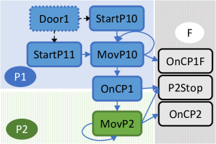
(a) For $0$-line

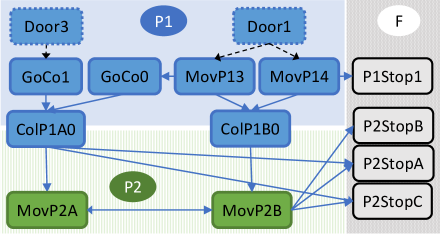
(b) For $(L-2)$-line and $(L-3)$-line

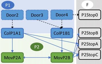
(c) For $(L-1)$-line

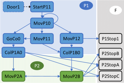
(d) For other lines

Figure 19: View type transitions of Algorithm 2. Each solid arrow (resp. dotted arrow) represents a transition by a Move (resp. Enter_Grid) operation. We omitted the view Door0.

By Lemma 16, distances between any two occupied nodes are two. Thus, by the same discussion as Theorem 3.1, we are now able to state our main result:

Theorem 3.3

Algorithm 2 constructs a maximum independent set by occupied locations on the grid.

By the proofs of Lemmas 14–16, nodes on the even-numbers (resp. odd-numbers) lines are occupied by $\lceil l/2\rceil$ (resp. $\lfloor l/2\rfloor$) robots. By the same discussion as Lemma 7, the following lemma holds.

Lemma 18

When a maximum independent set is constructed, $\lceil n/2\rceil$ robots are on the grid.

Each robot $r_{i}$ sets its value $k_{i}$ at most once by Rule 0-1. By the same discussion of Theorem 3.2, the following theorem holds.

Theorem 3.4

The time complexity of Algorithm 2 is $O(n(L+l))$ steps.

4 Conclusion

We proposed two algorithms to construct a maximum independent set on an unknown size grid in the case that the Door node is connected to a corner node. One of our algorithms uses only three colors for each robot light and $\phi=2$, but it assumes port numbering. The other uses seven colors for each robot light and $\phi=3$, and it executes in a completely anonymous graph. Both of the time complexity are $O(n(L+l))$ steps.

Some interesting questions remain open:

• Are there any algorithms for the case where each robot has no light or two light colors? Following the results by Hesari et al. [23] for the continuous line setting, we conjecture their impossibility result for oblivious (a.k.a. no-light robots) can be extended to the discrete asynchronous and unoriented setting.

• Are there any algorithms for the case where the visibility range is less than two?

• Are there any algorithms for other assumptions of the Door node? For example, the Door node can be connected to another node, and there may be multiple Door nodes.

• Are there any algorithms that can tolerate maximum independent set reconfiguration in the case of robot crashes? We conjecture that, assuming a failing robot turns off its light (that is, crash failures can be detected by other robots), it is possible to extend our algorithm to adjust the remaining robots and introduce new ones so that the maximum independent set is reconstructed.

Additionally, we plan to design algorithms for the case of a maximal independent set placement, and minimum dominating set placement, that requires fewer robots.

References

- [1] Adhikary, R., Bose, K., Kundu, M.K., Sau, B.: Mutual visibility by asynchronous robots on infinite grid. In: ALGOSENSORS. pp. 83–101 (2018)
- [2] Balabonski, T., Courtieu, P., Pelle, R., Rieg, L., Tixeuil, S., Urbain, X.: Continuous vs. discrete asynchronous moves: A certified approach for mobile robots. In: NETYS. pp. 93–109 (2019)
- [3] Barrière, L., Flocchini, P., Barrameda, E.M., Santoro, N.: Uniform scattering of autonomous mobile robots in a grid. Int. J. Found. Comput. Sci. 22(3), 679–697 (2011)
- [4] Bonnet, F., Milani, A., Potop-Butucaru, M., Tixeuil, S.: Asynchronous exclusive perpetual grid exploration without sense of direction. In: OPODIS. pp. 251–265 (2011)
- [5] Bose, K., Adhikary, R., Kundu, M.K., Sau, B.: Arbitrary pattern formation on infinite grid by asynchronous oblivious robots. Theor. Comput. Sci. 815, 213–227 (2020)
- [6] Bramas, Q., Devismes, S., Lafourcade, P.: Infinite grid exploration by disoriented robots. In: SIROCCO. pp. 340–344 (2019)
- [7] Bramas, Q., Tixeuil, S.: The random bit complexity of mobile robots scattering. Int. J. Found. Comput. Sci. 28(2), 111–134 (2017)
- [8] Casteigts, A., Albert, J., Chaumette, S., Nayak, A., Stojmenovic, I.: Biconnecting a network of mobile robots using virtual angular forces. Comput. Commun. 35(9), 1038–1046 (2012)
- [9] Clément, J., Défago, X., Potop-Butucaru, M.G., Izumi, T., Messika, S.: The cost of probabilistic agreement in oblivious robot networks. Inf. Process. Lett. 110(11), 431–438 (2010)
- [10] Cohen, R., Peleg, D.: Local spreading algorithms for autonomous robot systems. Theor. Comput. Sci. 399(1-2), 71–82 (2008)
- [11] D’Angelo, G., Stefano, G.D., Klasing, R., Navarra, A.: Gathering of robots on anonymous grids and trees without multiplicity detection. Theor. Comput. Sci. 610, 158–168 (2016)
- [12] Das, S., Flocchini, P., Prencipe, G., Santoro, N., Yamashita, M.: Autonomous mobile robots with lights. Theor. Comput. Sci. 609, 171–184 (2016)
- [13] Datta, A.K., Lamani, A., Larmore, L.L., Petit, F.: Ring exploration with oblivious myopic robots. In: SAFECOMP. pp. 335–342 (2013)
- [14] Devismes, S., Lamani, A., Petit, F., Raymond, P., Tixeuil, S.: Optimal grid exploration by asynchronous oblivious robots. In: SSS. pp. 64–76 (2012)
- [15] Devismes, S., Lamani, A., Petit, F., Raymond, P., Tixeuil, S.: Terminating exploration of a grid by an optimal number of asynchronous oblivious robots. The Computer Journal (2020)
- [16] Dieudonné, Y., Petit, F.: Scatter of robots. Parallel Process. Lett. 19(1), 175–184 (2009)
- [17] Flocchini, P.: Uniform Covering of Rings and Lines by Memoryless Mobile Sensors, pp. 2297–2301. Springer (2016)
- [18] Flocchini, P., Prencipe, G., Santoro, N.: Self-deployment of mobile sensors on a ring. Theor. Comput. Sci. 402(1), 67–80 (2008)
- [19] Flocchini, P., Prencipe, G., Santoro, N. (eds.): Distributed Computing by Mobile Entities, Current Research in Moving and Computing. Springer (2019)
- [20] Guilbault, S., Pelc, A.: Gathering asynchronous oblivious agents with local vision in regular bipartite graphs. Theor. Comput. Sci. 509, 86–96 (2013)
- [21] Hector, R., Vaidyanathan, R., Sharma, G., Trahan, J.L.: Optimal convex hull formation on a grid by asynchronous robots with lights. In: IPDPS. pp. 1051–1060 (2020)
- [22] Heriban, A., Défago, X., Tixeuil, S.: Optimally gathering two robots. In: ICDCN. pp. 3:1–3:10 (2018)
- [23] Hesari, M.E., Flocchini, P., Narayanan, L., Opatrny, J., Santoro, N.: Distributed barrier coverage with relocatable sensors. In: SIROCCO. pp. 235–249 (2014)
- [24] Hideg, A., Lukovszki, T.: Asynchronous filling by myopic luminous robots. Tech. rep., arXiv (2020)
- [25] Hsiang, T.R., Arkin, E.M., Bender, M.A., Fekete, S.P., Mitchell, J.S.B.: Algorithms for Rapidly Dispersing Robot Swarms in Unknown Environments, pp. 77–93. Springer (2004)
- [26] Kamei, S., Lamani, A., Ooshita, F.: Asynchronous ring gathering by oblivious robots with limited vision. In: WSSR. pp. 46–49 (2014)
- [27] Kamei, S., Lamani, A., Ooshita, F., Tixeuil, S., Wada, K.: Gathering on rings for myopic asynchronous robots with lights. In: OPODIS (2019)
- [28] Kshemkalyani, A., Molla, A.R., Sharma, G.: Dispersion of mobile robots on grids. In: WALCOM (2020)
- [29] Nagahama, S., Ooshita, F., Inoue, M.: Ring exploration of myopic luminous robots with visibility more than one. In: SSS. pp. 256–271 (2019)
- [30] Ooshita, F., Tixeuil, S.: Ring exploration with myopic luminous robots. In: SSS. pp. 301–316 (2018)
- [31] Poudel, P., Sharma, G.: Fast uniform scattering on a grid for asynchronous oblivious robots. In: SSS (2020)
- [32] Suzuki, I., Yamashita, M.: Distributed anonymous mobile robots: Formation of geometric patterns. SIAM Journal on Computing 28(4), 1347–1363 (1999)
- [33] Viglietta, G.: Rendezvous of two robots with visible bits. In: ALGOSENSOR. pp. 291–306 (2013)
- [34] Yamauchi, Y.: A survey on pattern formation of autonomous mobile robots: asynchrony, obliviousness and visibility. Journal of Physics: Conference Series 473, 012016 (2013)