Instantons for rare events in heavy-tailed distributions

Abstract

Large deviation theory and instanton calculus for stochastic systems are widely used to gain insight into the evolution and probability of rare events. At its core lies the realization that rare events are, under the right circumstances, dominated by their least unlikely realization. Their computation through a saddle-point approximation of the path integral for the corresponding stochastic field theory then reduces an inefficient stochastic sampling problem into a deterministic optimization problem: finding the path of smallest action, the instanton. In the presence of heavy tails, though, standard algorithms to compute the instanton critically fail to converge. The reason for this failure is the divergence of the scaled cumulant generating function (CGF) due to a non-convex large deviation rate function. We propose a solution to this problem by “convexifying” the rate function through a nonlinear reparametrization of the observable, which allows us to compute instantons even in the presence of super-exponential or algebraic tail decay. The approach is generalizable to other situations where the existence of the CGF is required, such as exponential tilting in importance sampling for Monte-Carlo algorithms. We demonstrate the proposed formalism by applying it to rare events in several stochastic systems with heavy tails, including extreme power spikes in fiber optics induced by soliton formation.

I Introduction

In many situations of physical relevance, rare events are tremendously important despite their infrequent occurrence: Heat waves, stock market crashes, or earth quakes all occur with small probability but devastating consequences. Unfortunately, due to their rareness, these events are hard to observe in experiment or numerical simulation, and require special treatment. Rare event algorithms Bucklew (2013) are typically based on one of the two following ideas: Either to increase the rate of occurrence of the rare event by biasing the underling system (importance sampling), or to substitute all possible ways of observing a rare event by its most common realization (large deviations/instanton theory). Under the hood both are connected to the exponentially tilted measure and the cumulant generating function. As we will see, when naively implementing standard schemes, both become ill-defined when the underlying probability densities become heavy-tailed.

Here, we focus on numerical algorithms connected to instanton theory and its rigorous counterpart, large deviation theory, to recover the tails of probability distributions in a stochastic system. A large deviation principle (LDP) states that the probability of rare events decays exponentially, and its exponential scaling is given by the minima of the corresponding rate function $I$ Varadhan (1966); Dembo and Zeitouni (2010). More precisely, let $P^{\varepsilon}$ be a family of probability measures on a suitable space $\mathcal{X}$. We say $P^{\varepsilon}$ satisfies an LDP with rate function $I:\Omega\to\mathds{R}$ if for all $\Omega\subset\mathcal{X}$, we have Freidlin and Wentzell (2012),

$$P^{\varepsilon}\left(\Omega\right)\asymp\exp\left(-\varepsilon^{-1}\,\inf\limits_{x\in\Omega}I\left(x\right)\right),$$ (1)

where $\asymp$ denotes log-asymptotic equivalence in the limit $\varepsilon\to 0$.

In a physical sense, the probability $P^{\varepsilon}(\Omega)$ can formally be written as a path integral, and the estimate (1) becomes a saddle point approximation or Laplace method. In large deviation theory, the Gärtner-Ellis theorem Ellis et al. (1984) provides a direct formula for the rate function $I$. Roughly speaking, if the limiting behavior of a scaled CGF is well-defined, then its Legendre-Fenchel (LF) transform is the rate function of the LDP of the process under consideration. The LF transform of a real-valued function $f\left(x\right)$ defined on $\mathds{R}^{n}$ is defined as

$$f^{*}\left(y\right)=\sup\limits_{x\in\mathds{R}^{n}}\left(\left\langle x,y\right\rangle-f\left(x\right)\right),$$ (2)

where $\left\langle x,y\right\rangle=x^{T}\,y$ is the inner product on $\mathds{R}^{n}$. Let $z^{\varepsilon}$ be a sequence of random variables in $\mathds{R}^{n}$, with probability measures $P^{\varepsilon}$, and assume that its scaled CGF, defined as the limit,

$$G\left(\lambda\right)\equiv\lim\limits_{\varepsilon\to 0}\,\varepsilon\log\,\mathbb{E}\left[e^{\varepsilon^{-1}\langle\lambda,z^{\varepsilon}\rangle}\right],$$ (3)

exists for each $\lambda\in\mathds{R}^{n}$ and is differentiable in $\lambda$. Then, the Gärtner-Ellis theorem states that the family of probability measures $\left\{P^{\varepsilon}\right\}$ satisfy an LDP, where the rate function $I$ is the LF transform of $G$, $I=G^{*}$.

Intuitively, one can interpret $\lambda$ as a Lagrange multiplier to condition on an outcome $z$. Crucially, though, if the probability measure $P^{\varepsilon}$ is super-exponential, or has even heavier tails, the expectation in equation (3) diverges and the CGF is no longer defined. Notably this does not mean that the corresponding rare events are special in any way, but merely that the duality between the parameter $\lambda$ and rare event observable $z$ is broken. As a consequence, no tilt exists to realize an outcome $z$, and standard rare events algorithms fail.

In what follows, we will show how a nonlinear tilt allows to modify the connection between tilt $\lambda$ and outcome $z$, so that heavy tails can be probed regardless of the non-convexity of their rate function. We will concentrate specifically on the case of small noise sample-path large deviations for stochastic differential equations (SDEs), which will we introduced in section II. Here, we focus on the numerical computation of the instanton in section II.1, and highlight the connection to a change of measure in path-space in II.2. We demonstrate the problem in the heavy-tailed case by reviewing the convex analysis for the Gärtner-Ellis theorem in section III, and propose a solution modifying the instanton computation to yield finite outcomes for heavy tails and non-convex rate functions in section III.1. To demonstrate the applicability of our approach, we show several examples of instantons for heavy-tailed distributions in section IV: Toy models with super-exponential (section IV.1) and powerlaw (section IV.2) tails, and a banana-shaped potential (section IV.3), and finally high-amplitude events in fiber-optics described by the focusing nonlinear Schrödinger equation (section IV.4). We summarize our findings in section V.

II Instantons and Freidlin-Wentzell theory

Consider a stochastic system,

$$dX^{\varepsilon}_{t}=b\left(X^{\varepsilon}_{t}\right)\,dt+\sqrt{\varepsilon}\sigma\,dW_{t}\,,\quad X^{\varepsilon}_{t_{0}}=x_{0},$$ (4)

where $X^{\varepsilon}_{t}\in\mathds{R}^{n}$ is a family of random processes indexed by the noise strength $\varepsilon$. The deterministic drift $b:\mathds{R}^{n}\to\mathds{R}^{n}$ satisfies the Lipschitz condition, $dW_{t}$ is an $n$-dimensional Brownian increment, and the noise covariance $\chi=\sigma\sigma^{T}$ is assumed to be invertible for $\sigma\in\mathds{R}^{n\times n}$. Intuitively, equation (4) describes the temporal evolution of a system perturbed by stochasticity, where we later assume the fluctuations to be small, $\varepsilon\ll 1$. This situation is ubiquitous in many application areas, where for example $\varepsilon$ plays the role of the temperature in a chemical reaction, or the inverse number of particles in a thermodynamic system.

With vanishing noise, $\varepsilon=0$, the solution $x\in\mathds{R}^{n}$ of the unperturbed (deterministic) system

$$\dot{x}(t)=b\left(x(t)\right),\,\,\,\,x(t_{0})=x_{0},$$ (5)

converges to one of its attractors for long times. For example, consider a point attractor, or asymptotically stable fixed points, $\bar{x}\in\mathds{R}^{n}$, with basin of attraction $B$, such that $x(t)\to\bar{x}$ for $t\to\infty$ for all initial conditions $x_{0}$ in $B$. Solutions of the stochastic system (4) converge to solutions of the deterministic system (5) in probability, $P(\lim\limits_{\varepsilon\rightarrow 0}\,\max\limits_{t_{0}\leq t\leq t_{1}}\left|X^{\varepsilon}_{t}-x(t)\right|=0)=1$  Freidlin and Wentzell (2012). This is an instance of the law of large numbers, stating that for small noise and large times we expect solutions of the stochastic system to end up near the attractors of the deterministic one.

Nevertheless, for any non-zero $\varepsilon\ll 1$ there is a small but non-vanishing probability of finding the system far from the attractor. This can only happen if the noise conspires in just the right way to overcome the deterministic dynamics, and is consequently a rare event. Concretely, consider any domain $D\subset\mathds{R}^{n}$ attracted to $\bar{x}$, i.e. $D\subset B$. We are interested in the chance of trajectories $X_{t}^{\varepsilon}$ departing from $\bar{x}$ and eventually leaving $D$. These trajectories belong to the set

$$A_{z}\coloneqq\left\{\varphi\in\textbf{C}_{t_{0}\,t_{1}}\left(\mathds{R}^{n}\right)|\varphi(t_{0})=\bar{x},\varphi(t_{1})=z\notin D\right\},$$ (6)

and we want to quantify the probability

$$p(z)=P\left[X^{\varepsilon}\in A_{z}\right]\quad\text{as}\quad\varepsilon\rightarrow 0\,,$$ (7)

which is a question about the probability of large deviations. Under the stated conditions, there is a trajectory $\varphi^{*}\in A_{z}$ such that the probability measure over $A_{z}$ accumulates near $\varphi^{*}$ for $\varepsilon\to 0$, namely if $N\left(\varphi^{*}\right)$ is any neighborhood of $\varphi^{*}$,

$$\lim\limits_{\varepsilon\rightarrow 0}\,\frac{P\left[X^{\varepsilon}\in A_{z}\setminus N\left(\varphi^{*}\right)\right]}{P\left[X^{\varepsilon}\in N\left(\varphi^{*}\right)\right]}=0.$$ (8)

In other words, in the small noise limit we will almost surely find our sample trajectory close to $\varphi^{*}$, such that ${\max\limits_{t_{0}\leq t\leq t_{1}}\left|X^{\varepsilon}_{t}-\varphi^{*}_{t}\right|\leq\delta}$, for an arbitrary small $\delta$.

In order to find this most likely trajectory $\varphi^{*}$, Freidlin-Wentzell theory Freidlin and Wentzell (2012) states that $\varphi^{*}$ is actually the minimizer of large deviation rate function $S(\varphi)$ associated with the stochastic system (4), given by

$$S(\varphi)=\frac{1}{2}\int_{t_{0}}^{t_{1}}\left\|\dot{\varphi}_{t}-b\left(\varphi(t)\right)\right\|_{\chi}^{2}dt,$$ (9)

where the integral exists, and $S(\varphi)=\infty$ otherwise. The norm $\left\|f\right\|_{\chi}^{2}=\left\langle f,\chi^{-1}f\right\rangle$ is induced by the noise covariance $\chi$. With this rate function we can quantify the probability (7) of departing the domain $D$ as

$$\lim\limits_{\varepsilon\rightarrow 0}\,\varepsilon\,\log\,p(z)=-I(z)=-S\left(\varphi^{*}\right)\,,$$ (10)

where

$$\varphi^{*}=\underset{\varphi\in A_{z}}{\mathrm{argmin}}\,S\left(\varphi\right)\,.\\$$ (11)

The problem of finding the rare event probability is now reduced to finding the minimizer $\varphi^{*}$.

In analogy to the principle of least action in classical mechanics or quantum mechanics, the rate function is often termed action, and the corresponding minimizer $\varphi^{*}$ is called instanton. The integrand of $S$ can be understood as a Lagrangian,

$$L\left(\varphi,\dot{\varphi}\right)=\frac{1}{2}\left\|\dot{\varphi}_{t}-b\left(\varphi\right)\right\|_{\chi}^{2},$$ (12)

so that the maximum likelihood pathways leaving the attractors of (4) correspond to semi-classical trajectories of the field theory defined by $L$.

II.1 Instanton equations and large deviation Hamiltonian

It is helpful, both to increase understanding, and to simplify the numerical implementation, to rephrase the optimization problem (11) into the corresponding Hamiltonian formulation. To this end, we introduce the large deviation Hamiltonian $H(\varphi,\vartheta)$ as the Legendre transform of the Lagrangian $L\left(\varphi,\dot{\varphi}\right)$,

$$H\left(\varphi,\vartheta\right)=\sup\limits_{\dot{\varphi}}\left(\left\langle\vartheta,\,\dot{\varphi}\right\rangle-\textit{L}\left(\varphi,\dot{\varphi}\right)\right)\,,$$ (13)

which, for the Lagrangian (12), corresponds to

$$H(\varphi,\vartheta)=\langle b(\varphi),\vartheta\rangle+\tfrac{1}{2}\langle\vartheta,\chi\vartheta\rangle\,.$$ (14)

Here $\vartheta=\partial L/\partial\dot{\varphi}$ is the conjugate momentum of $\varphi$ Deriglazov (2017). Now, the minimizer $\varphi^{*}$ can also be expressed as the solution of Hamilton’s equations,

$$\begin{split}\dot{\varphi}&=\partial_{\vartheta}H(\varphi,\vartheta)=b\left(\varphi\right)+\chi\ \vartheta,\\ \dot{\vartheta}&=-\partial_{\varphi}H(\varphi,\vartheta)=-\left(\nabla_{\varphi}b\left(\varphi\right)\right)^{T}\,\vartheta.\end{split}$$ (15)

with boundary conditions,

$$\varphi(t_{0})=\bar{x},\qquad\varphi(t_{1})=z.$$ (16)

Equations (15) and (16) are often termed instanton equations.

The fact that we are looking only for trajectories that will eventually leave the attractor, $\varphi^{*}\in A_{z}$, implies that the optimization problem (11) is a constrained one, i.e. we are looking only for solutions of the instanton equations conditioned on the endpoint $z$. Practically, this constrained optimization problem can be transformed into an unconstrained one,

$$\varphi^{*}=\underset{\varphi\in\textbf{C}_{t_{0}\,t_{1}}\left(\mathds{R}^{n}\right)}{\mathrm{argmin}}\left(S\left(\varphi\right)-\left\langle\lambda,\ \varphi(t_{1})-z\right\rangle\right),$$ (17)

by using a Lagrange multiplier $\lambda\in\mathds{R}^{n}$ to enforce the final constraint Rindler (2018). Note that the variation of this unconstrained action,

$$\left[\delta S\left(\varphi\right)-\left\langle\lambda,\,\delta\varphi(t_{1})\right\rangle\right]_{\varphi=\varphi^{*}}=0,$$ (18)

results in the same instanton equations,(15), but with different boundary conditions

$$\varphi\left(t_{0}\right)=0,\quad\vartheta\left(t_{1}\right)=\lambda.$$ (19)

We can solve the instanton equations (15) iteratively with these conditions, by solving the $\varphi$-equation forward in time, and using the result to solve the $\vartheta$-equation backward in time, until convergence Chernykh and Stepanov (2001); Grafke et al. (2014). Note that this choice of temporal direction of integration is not only the one suggested by the boundary conditions, but is further the numerically stable choice of direction for the drifts $b$ and $\nabla b^{T}$.

As we will see below, the mapping between Lagrange multipliers $\lambda$ and final points $z$ is nontrivial, and it is not clear a priori how to choose the correct $\lambda$ to obtain a final configuration $z=\varphi^{*}(t_{1})$. If we are interested in $p^{\varepsilon}(z)$ for a whole range of $z$, we can instead choose to simply solve the instanton equations for a range of $\lambda$ to cover a range of $z$ without specifically needing to know the duality mapping $\lambda(z)$. Exactly this procedure is often used in the literature to work out probability distributions of stochastic systems, from Burgers Chernykh and Stepanov (2001); Grafke et al. (2013) or Ginzburg-Landau Rolland et al. (2016) equations to the Kardar-Parisi-Zhang Meerson et al. (2016) and Kipnis-Marchioro-Presutti model Zarfaty and Meerson (2016)

Crucially, however, the existence of a corresponding dual $\lambda$ for a given final point $z=\varphi^{*}\left(t_{1}\right)$ is not necessarily guaranteed, as the next section clarifies. As a consequence, the above methodology might fail, in particular in situations with heavy tails.

II.2 Exponentially tilted measures

Interestingly, there is a probabilistic interpretation of the introduction of the Lagrange multiplier $\lambda$ to the optimization problem (18) in the form of the exponentially tilted measure Touchette (2009); Cohen and Elliott (2015), as for example employed in importance sampling for Monte-Carlo estimators Bucklew (2013). Intuitively, by the procedure of tilting, one replaces the original random process (4) by a modified one, under which the rare events under consideration become more likely, while correcting for this modification a posteriori when computing their probability. As a consequence, with tilting, the rare event probability, or expectations over its realizations, can be estimated more efficiently, and with possibly smaller variance.

To be more precise, we denote by $p_{\lambda}$ the measure exponentially tilted towards the outcome $z$, defined for our purposes as

$$p_{\lambda}(z)=\frac{\exp\left(\varepsilon^{-1}\left\langle\lambda,\,z\right\rangle\right)}{\mathop{\mathbb{E}}_{p}\left[\exp\left(\varepsilon^{-1}\left\langle\lambda,\,z\right\rangle\right)\right]}\,p\left(z\right),$$ (20)

where $\mathop{\mathbb{E}}_{p}\left[.\right]$ is the expectation under the original measure $p$. In equation (20), the probability measure $p_{\lambda}$ of events resulting in $z$, i.e. trajectories in $A_{z}$, have been awarded extra weight by the Radon-Nikodym derivative of $p_{\lambda}$ with respect to $p$, which is:

$$\frac{p_{\lambda}\left(z\right)}{p\left(z\right)}=\frac{dp_{\lambda}\left(z\right)}{dp\left(z\right)}=\frac{\exp\left(\varepsilon^{-1}\left\langle\lambda,\,z\right\rangle\right)}{\mathop{\mathbb{E}}_{p}\left[\exp\left(\varepsilon^{-1}\left\langle\lambda,\,z\right\rangle\right)\right]}.$$ (21)

Rearranging equation (20) gives:

$$p_{\lambda}\left(z\right)=\exp\left(\varepsilon^{-1}\,\left\{\left\langle\lambda,\,z\right\rangle-G\left(\lambda\right)\right\}\right)\,p\left(z\right),$$ (22)

where

$$G\left(\lambda\right)=\varepsilon\,\log\,\mathbb{E}_{p}\left[\exp\left(\varepsilon^{-1}\left\langle\lambda,\,z\right\rangle\right)\right]$$ (23)

is the scaled CGF, $G:\mathds{R}^{n}\to\mathds{R}$. This change of measure is optimal, in the sense of maximizing the tilted probability $p_{\lambda}$, at the choice $\lambda=\lambda_{z}$ with

$$\lambda_{z}=\underset{\lambda\in\mathds{R}^{n}}{\mathrm{argmax}}\left\{\left\langle\lambda,\,z\right\rangle-G\left(\lambda\right)\right\}.$$ (24)

This can be seen, given the Gärtner-Ellis theorem, $I(z)=G(\lambda)^{*}=\sup_{\lambda\in\mathds{R}^{n}}(\langle\lambda,z\rangle-G(\lambda))$, by realizing that

$$\begin{split}\log p_{\lambda}\left(z\right)&=\varepsilon^{-1}\,\left(\left\langle\lambda_{z},\,z\right\rangle-G\left(\lambda_{z}\right)\right)\,+\,\log p\left(z\right)\\ &=\varepsilon^{-1}\,\underset{\lambda\in\mathds{R}^{n}}{\mathrm{sup}}\left\{\left\langle\lambda,\,z\right\rangle-G\left(\lambda\right)\right\}\,+\,\log p\left(z\right)\\ &=\varepsilon^{-1}\,I\left(z\right)\,+\,\log p\left(z\right)\\ &\stackrel{{\scriptstyle\varepsilon\to 0}}{{\longrightarrow}}0,\end{split}$$ (25)

where the last line is just the definition of the LDP, $\varepsilon\log p(z)=-I(z)$ for $\varepsilon\to 0$.

It is in this sense that the optimal tilting parameter of the end-point distribution corresponds to the Lagrange multiplier in the instanton equations constraining the endpoint to $z$.

III Convex analysis and the Gärtner-Ellis theorem

In order to use the described methodology to find the instanton for a rare outcome $z$, or equivalently make sense of the corresponding exponentially tilted measure $p_{\lambda}(z)$, we must demand that the mapping $z\to\lambda(z)$ is a bijection: For every outcome $z$ there must be a unique tilt $\lambda$ such that the instanton $\varphi$, solution of (15) with boundary conditions (19) have a unique solution with $\varphi(t_{1})=z$. If that is the case then we can estimate the probability

$$p(z)\asymp\exp(-\varepsilon^{-1}S(\varphi^{*}))=\exp(-\varepsilon^{-1}I(z))\,.$$ (26)

The precise properties of the duality mapping between tilting parameter $\lambda$ and outcome $z$ can be understood by the interplay between the Gärtner-Ellis theorem and convex analysis. We have,

$$\begin{split}G\left(\lambda\right)&=\sup\limits_{z\in\mathds{R}^{n}}\left(\left\langle\lambda,\,\,z\right\rangle-I\left(z\right)\right)\\ &=\left\langle\lambda,\,\,z\left(\lambda\right)\right\rangle-I\left(z\left(\lambda\right)\right),\end{split}$$ (27)

where the solution $z\left(\lambda\right)$ of the form

$$\nabla I\left(z\right)=\lambda\,,$$ (28)

does only hold when the rate function is strictly convex. If instead the rate function is not strictly convex (i.e. has concave, and/or affine linear regions or is even just asymptotically linear), the LF transform is applied only to the region at which $I\left(z\right)$ admits supporting hyperplanes. If there exists $\lambda\in\mathds{R}^{n}$ such that Touchette (2005),

$$I\left(y\right)\geq I\left(z\right)+\lambda\left(y-z\right),\ \ \forall y\in\mathds{R}^{n},$$ (29)

then we say $I$ admits a supporting hyperplane at $z$, where the slope of the supporting hyperplane is $\lambda$. In this sense, we can define non-convex regions to be the ones that do not admit any supporting hyperplane, so do not have any corresponding $\lambda$. Note that the absence of these hyperplanes can affect the LF transform $I^{*}\left(z\right)=G\left(\lambda\right)$ in two different ways,

1. Having an asymptotically linear part of $I\left(z\right)$ leads to a divergent LF transform $G\left(\lambda\right)$.

2. Having a concave or affine linear part of $I\left(z\right)$ leads to an existent but nondifferentiable LF transform $G\left(\lambda\right)$.

Both cases will be discussed specifically in the applications in section IV.

Assuming for now there are supporting hyperplanes (i.e. existent $\lambda$) for all $z\in\mathds{R}^{n}$, then equation (28) leads to,

$$z\left(\lambda\right)=\left(\nabla I\right)^{-1}\left(\lambda\right),$$ (30)

i.e. $\nabla I$ must be invertible for $z(\lambda)$ to be so. Up to a choice of sign, this implies that $\nabla I$ is strictly monotonically increasing (SMI), which is equivalent to $I$ being a strictly convex function Touchette (2009). Also note that if $z\left(\lambda\right)$ is invertible, this implies that $G\left(\lambda\right)$ is a differentiable function, since equation (27) gives,

$$\begin{split}\nabla G\left(\lambda\right)&=z\left(\lambda\right)\,+\left(\nabla z\left(\lambda\right)\right)^{T}\,\,\lambda-\left(\nabla z\left(\lambda\right)\right)^{T}\nabla I\left(z\left(\lambda\right)\right)\\ &=z\left(\lambda\right),\end{split}$$ (31)

where equation (28) is used. What we have demonstrated above is nothing but the well-known fact that the LF transform of a convex, differentiable function $G(\lambda)$ is strictly convex. This perspective, though, makes it clear that the existence of a tilting parameter (Lagrange multiplier) $\lambda$ to enforce an outcome $z$ depends on the finiteness and differentiability of the scaled CGF. In other words, both exponential tilting, and finding a Lagrange parameter to constrain the endpoint to $z$, depends on the rate function being strictly convex.

Since in the low noise limit we have $p(z)\sim\exp(-\varepsilon^{-1}I(z))$, it is easy to construct cases where the rate function $I(z)$ is not strictly convex. In fact, every situation where the tails of $p(z)$ are fat, i.e. exponential ($I(z)\sim z$), stretched exponential ($I(z)\sim z^{\alpha},\alpha<1$), or even algebraic ($I(z)\sim\alpha\log(z),\alpha<0$) tails will break the above assumption. Examples of fat tailed distributions are ubiquitous in physical systems of relevance, such as the energy dissipation in fluid turbulence and the phenomenon of intermittency Frisch (1995), wealth distributions in economies Drăgulescu and Yakovenko (2001); Sinha (2006) or stock price changes in finance Gopikrishnan et al. (2000); Plerou et al. (2000).

The main contribution of this paper is the realization that the introduction of a nonlinear map $F:\mathds{R}^{n}\to\mathds{R}^{n}$ allows us to loosen the restriction of the convexity of $I(z)$. The idea is to define a nonlinear tilt through $F$ via $\exp(\varepsilon^{-1}\langle\lambda,F(z)\rangle)$, such that the map $\lambda\to z(\lambda)$ is replaced by a new map $\lambda\to F\circ z(\lambda)$. We are free to choose any appropriate $F$. As we will see next, this allows us to suitably reparametrize the space of outcomes, so that the effective rate function $I\circ F^{-1}$ is strictly convex.

III.1 Nonlinear tilt

In analogy to equation (22) and the description in sections II.2 and III, we can now define the nonlinearly tilted measure

$$\begin{split}p_{\lambda}^{F}(z)&=\frac{\exp(\varepsilon^{-1}\langle\lambda,F(z)\rangle)}{\mathbb{E}_{p}\exp(\varepsilon^{-1}\langle\lambda,F(z)\rangle)}p(z)\\ &=\exp\left(\varepsilon^{-1}(\langle\lambda,F(z)\rangle-G_{F}(\lambda))\right)\,p(z)\end{split}$$ (32)

where the nonlinearly tilted CGF is given by

$$\begin{split}G_{F}\left(\lambda\right)&=\sup\limits_{z\in\mathds{R}^{n}}\left(\left\langle\lambda,\,F\left(z\right)\right\rangle-I\left(z\right)\right)\\ &=\left\langle\lambda,\,F\left(z\left(\lambda\right)\right)\right\rangle-I\left(z\left(\lambda\right)\right),\end{split}$$ (33)

(compare equation (27)) which is assumed to be finite and differentiable. Its gradient fulfills

$$\begin{split}\nabla G_{F}\left(\lambda\right)&=F\left(z\left(\lambda\right)\right)+\left(\nabla z(\lambda)\right)^{T}\left(\nabla F(z(\lambda))\right)^{T}\,\,\lambda\\ &-\left(\nabla z(\lambda)\right)^{T}\nabla I(z(\lambda))\\ &=F\left(z\left(\lambda\right)\right),\end{split}$$ (34)

where the last equality is due to $z\left(\lambda\right)$ being the solution of $\nabla I\left(z\right)=\lambda^{T}\nabla F(z)$ in equation (LABEL:eq:G_F).

This proposed remapping can be chosen to overcome the above problem by creating a new function $G_{F}\left(\lambda\right)$, which plays the role of the CGF, while simultaneously being a bounded and differentiable function. At the same time, $I\circ F^{-1}\left(y\right)$ can be understood as the effective rate function, since equation (LABEL:eq:G_F) can be written as,

$$G_{F}\left(\lambda\right)=\sup\limits_{F^{-1}\left(y\right)\in\mathds{R}^{n}}\left(\left\langle\lambda,\,y\right\rangle-I\circ F^{-1}\left(y\right)\right).$$ (35)

Obviously, the right choice of $F$ depends on the nature of the tail scaling at hand. We will derive the necessary properties of $F\left(.\right)$ next.

III.2 Properties of the reparametrization and the nonlinearly tilted instanton

In the following, we denote by $y\in\mathds{R}^{n}$ the reparametrized outcome, $y=F(z)$. Our goal is to choose $F$ such that $F\circ z(\lambda)=y(\lambda)$ is a bijection. From above, it is clear that

$$\lambda^{T}=\nabla I(z)(\nabla F(z))^{-1}\,.$$ (36)

Following the same argument as in section III, $y(\lambda)$ is bijective if

• $F$ is a diffeomorphism, and

• $I\circ F^{-1}(y)$ is strictly convex, i.e.

  $$\langle v,\mathrm{Hess}(I\circ F^{-1})(y)\,v\rangle>0\ \forall\ v\in\mathds{R}^{n}\,.$$ (37)

Assuming these conditions on $F$ implies that the gradient of the reparametrized rate function ${I\circ F^{-1}(y)}$, given by $\lambda\circ F^{-1}\left(y\right)$, is an SMI function, implying that it is invertible. The desired bijective mapping then becomes ${\lambda\rightarrow F\left(z\left(\lambda\right)\right)=\nabla G_{F}\left(\lambda\right)}$ (compare equation (34)). For a non-convex $I$, intuitively, $F$ must be chosen to suitably reparametrize the space of outcomes for the effective rate function to become strictly convex. For example for the $n=1$ case with heavy tails, one might imagine a strong enough compression of the observable $z$ such that a fat tail becomes non-fat.

To harness this nonlinear tilt in the computation of instantons for distributions with heavy tails, we need to modify the approach outlined in section II.1 as follows: The variation of the unconstrained action (18) now reads

$$\left[\delta S\left(\varphi\right)-\left\langle\lambda,\,\nabla F(\varphi(t_{1}))\delta\varphi(t_{1})\right\rangle\right]_{\varphi=\varphi^{*}}=0\,.$$ (38)

Consequently, the boundary conditions of the instanton equations are modified to

$$\varphi\left(t_{0}\right)=0,\quad\vartheta\left(t_{1}\right)=\lambda\nabla F(\varphi(t_{1}))\,,$$ (39)

which will yield an instanton trajectory $\varphi^{*}$ that reaches $z$, $\varphi(t_{1})=z$, despite the fact that the rate function $I(z)=S(\varphi^{*})$ is not convex around $z$. Since $F$ is continuous, the probability measure $P^{\varepsilon}\circ F^{-1}\left(y\right)$ in the limit $\varepsilon\to 0$ is the same as $P^{\varepsilon}\left(z\right)$ for a continuous $F$, according to the contraction principle Freidlin and Wentzell (2012); Dembo and Zeitouni (2010).

Note that this reparametrization through $F$ is introduced solely to adequately define the tilted measure, or equivalently numerically compute the instanton without encountering divergences. Afterwards, the reparametrization can be reverted to obtain the probability distribution in the original coordinates $z$.

As additional remark, methods that compute the instanton by solving the global optimization problem, for example by solving the associated Euler-Lagrange equations instead of integrating the instanton equations E et al. (2004); Grafke et al. (2017), do not require the above treatment: The tilting parameter disappears in these cases as the boundary conditions are fixed in the field variable instead of the conjugate momentum. Therefore, in principle, these methods can be chosen in the non-convex case. The solution of the instanton equations, though, is generally preferred Grafke and Vanden-Eijnden (2019) due to numerically efficiency, and sometimes even required (such as when the noise covariance in (4) is not invertible).

IV Applications

We will now consider a number of examples that show how to compute tail probabilities in stochastic systems. To demonstrate the wide applicability of our approach, we consider several cases that highlight different complications. We start with two toy models that feature stretched exponential (section IV.1) or powerlaw (section IV.2) tails. Then, in section IV.3, we consider a two-dimensional system with a bent (“banana-shape”) potential, where the non-convexity is not due to heavy tails, but due to the shape of the unimodal invariant probability density. Lastly, we demonstrate the practical applicability of our method by considering an example motivated from fiber optics in section IV.4. Here we compute the probability of measuring extreme power spikes at the end of extended optical fibers, where the probability distribution of the input signal is known. Due to soliton formation, this distribution features heavy tails for long fiber lengths ($L\gg 10\ \textrm{m}$), so in order to compute probabilities via an instanton approach, our corrections are necessary.

IV.1 Stretched exponential

Consider the stochastic gradient flow,

$$dX^{\varepsilon}_{t}=-\nabla U(X^{\varepsilon}_{t})\,dt+\sqrt{2\,\varepsilon}\,\,dW_{t}\,,\quad t\in[t_{0},t_{1}]\,.$$ (40)

The potential $U:\mathds{R}^{n}\rightarrow\mathds{R}$ determines completely the stationary probability distribution function (PDF)

$$\rho_{\infty}(z)=Z^{-1}\exp\left(-\varepsilon^{-1}U\left(z\right)\right)$$ (41)

with normalization constant $Z$. We further assume that $U$ has a unique minimum, i.e. we are only considering unimodal distributions. For large times, $t_{1}-t_{0}=T\to\infty$, the distribution of endpoints of $X^{\varepsilon}_{t_{1}}=z$ will converge to $\rho_{\infty}(z)$. From the perspective of large deviation theory (LDT), comparing (26) to (41), the rate function for the final point distribution is equivalent to the potential, $I(z)=U(z)$, and

$$\lim\limits_{\varepsilon\rightarrow 0}\varepsilon\,\log\,p(z)= \,-U\left(z\right)\,.$$ (42)

Therefore, in order to approximate the tails of the stationary distribution, we can compute the instanton $\varphi^{*}$ ending at $z$ and estimate $\rho_{\infty}(z)\approx\exp(-\varepsilon^{-1}S(\varphi^{*}))$.

We choose $n=1$ and consider the non-convex potential,

$$U\left(z\right)=\left(\frac{z^{4}}{1+\left|z\right|^{3}}\right)^{\alpha}\,,\quad 0<\alpha\leq 1\,,$$ (43)

which corresponds to a stretched exponential stationary distribution: At the tails, the dominant exponent is $\alpha$, and $\rho_{\infty}(z)\approx\exp(-\varepsilon^{-1}\left|z\right|^{\alpha})$ for large $z$, as shown in figure 1. For this distribution, $\mathbb{E}[\exp(\varepsilon^{-1}\lambda z)]$ diverges for large $\lambda$ as in case I, and hence numerical methods to find the instanton fail in the tail.

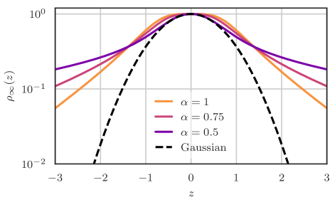
Figure 1: The potential ${U\left(z\right)=\left(z^{4}/(1+\left|z\right|^{3}\right)^{\alpha}}$, ${0<\alpha\leq 1}$, for the gradient flow SDE (40) leads to heavy (stretched exponential) tails of the stationary density $\rho_{\infty}(z)$ as $\alpha$ decreases.

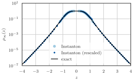
Figure 2: Stationary density with exponential tails (equation (43) for $\alpha=1$). Probing the tails with the traditional instanton method (light blue) leads to numerical divergence around the non-convex tail region. Reparametrizing the observable via $F(z)=\mathop{\mathrm{sign}}(z)\log\left|z\right|$ convexifies the tail, so that the instanton (dark blue) correctly predicts the exact tail probabilities (solid black).

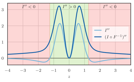
Figure 3: Convexity condition for the stretched exponential tails: The second derivative of the rate function becomes negative beyond the inflection points at $z\approx\pm 1.26$. The nonlinearly tilted rate function, instead, remains strictly convex in the whole domain, $(I\circ F^{-1})^{\prime\prime}>0$.

This can be seen in figure 2: We employ the numerical scheme by Chernykh-Stepanov Chernykh and Stepanov (2001); Grafke et al. (2013) to compute the instanton starting at $\varphi^{*}(t_{0})=0$ and ending at $\varphi^{*}(t_{1})=z$. The iterative algorithm converges towards the minimizer of the action, and once converged, we can estimate the probability of reaching $z$ by $p(z)\approx\exp(-\varepsilon^{-1}S(\varphi^{*}))$. As expected, though, computing the instanton fails beyond the inflection points at $z\approx\pm 1.26$, where the tails become stretched exponentials (light blue dots): No choice of $\lambda$ leads to endpoints $z$ of the instanton beyond these, as the linear tilt diverges and the CGF is undefined. Instead, we need to choose a non-linear tilt, such as

$$F(z)=\mathop{\mathrm{sign}}(z)\log\left|z\right|\,,\quad z\in\mathds{R}\setminus\{0\}\,,$$ (44)

for which even in the tails the reparametrized expectation $\mathbb{E}[\exp(\varepsilon^{-1}\lambda F(X^{\varepsilon}_{t_{1}}))]<\infty$ remains bounded. Consequently, the derivative of the CGF $G_{F}(\lambda)$ is a bijection, so that every value of $\lambda$ has a corresponding $z$. This map is explicitly given by

$$\lambda(z)=\lambda\circ F^{-1}\left(x\right)=e^{4x}\left(4+e^{3x}\right)/\left(1+e^{3x}\right)^{2}$$ (45)

(for $z>0$, and negative for $z<0$).

With this choice, the instanton prediction for the stationary PDF is almost exact far into the heavy tails (dark blue dots vs black solid in figure 2). Here, we again employ the iterative instanton computation, but are solving the instanton equations with the boundary condition (39) instead. The underlying reason for convergence is that the reparametrization with $F$ convexifies the rate function, i.e. creating supporting lines with slopes $\lambda$ for all the domain of $I\circ F^{-1}$. As shown in figure 3, while the second derivative of the rate function becomes negative beyond the inflection points, the second derivative of the nonlinearly tilted rate function remains positive throughout.

For the numerics in this example, we chose $\alpha=1$, with $N_{t}=10^{3}$ timesteps, and a time interval of $T=6$.

IV.2 Powerlaw distribution

Even heavier tails are given by power law distributions,

$$p(z)\sim|z|^{-\beta}\,,$$ (46)

which are associated with a multitude of phenomena in wide areas of science, in part due to their connection to scale invariance, self-similarity, universality classes and criticality in phase transitions. Here, we construct a simple SDE in $n=1$ dimensions which has a powerlaw invariant density. Consider

$$dX_{t}^{\varepsilon}=-\frac{\beta X_{t}^{\varepsilon}}{1+(X_{t}^{\varepsilon})^{2}}\,dt+\sqrt{2\varepsilon}\,dW_{t}\,.$$ (47)

It can easily be shown that the invariant density for the process (47) is given by

$$\rho_{\infty}(z)=Z^{-1}(1+z^{2})^{-\beta/2\varepsilon}\,,$$ (48)

where $Z$ is a normalization constant. For $z\gg 1$ and $\varepsilon=1$, this takes the limiting form (46), but is regularized for small $z$. Again, we are interested in computing tail probabilities for this toy model, by computing the instanton $\varphi^{*}$ realizing large values of $z$, which yields the respective probability by evaluating the corresponding action.

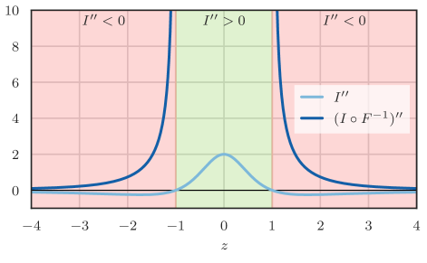
Figure 4: Convexity condition for the powerlaw test case: The second derivative of the rate function is negative in the tails beyond the inflection points at $z=\pm 1$ (light blue). The nonlinearly tilted rate function is strictly convex in this region instead (dark blue).

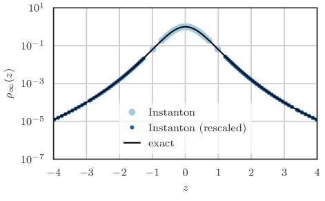
Figure 5: Stationary density with powerlaw tails ($\beta=2,\varepsilon=0.25$). Naively computing the instanton for tail events fails beyond $z=1$ (light blue). The nonlinear tilt $F(z)=\mathop{\mathrm{sign}}(z)\log\log|z|$ yields probabilities of events with $z\gg 1$ within the non-convex powerlaw tail (dark blue) in good agreement with the theoretical result (black solid).

As in section IV.1, the LDT rate function, given here by

$$I(z)=\tfrac{1}{2}\beta\log(1+z^{2})\,,$$ (49)

does not admit supporting lines in the tails, and consequently its LF transform is undefined (case I as well). This is reflected in the fact that the moment generating function

$$\mathbb{E}\exp(\varepsilon^{-1}\lambda z)=\int_{\mathds{R}}\exp(\varepsilon^{-1}\lambda z)(1+z^{2})^{-\beta/2\varepsilon}\,dz,$$ (50)

diverges. We can convexify the rate function (49) by reparametrizing via

$$F(z)=\mathop{\mathrm{sign}}(z)\log\log|z|\,,\quad z\in\mathds{R}\setminus[-1,1]\,,$$ (51)

which is an even more drastic tail compression than needed for the stretched exponential. Note that here we only convexify in the tails, $|z|>1$, where the problem occurs, and do not attempt to find a global map. Indeed, for this choice of $F$, the reparametrized rate function $I\circ F^{-1}(z)$ is convex in the tails, as shown in figure 4: Its second derivative remains positive in the tails, which is not true for the original rate function $I(z)$. We can explicitly map $\lambda$ to $z$ via

$$\lambda(z)=\lambda\circ F^{-1}\left(x\right)=\beta e^{\left(2e^{x}+x\right)}/\left(1+e^{2e^{x}}\right)$$ (52)

(for $z>1$ and negative for $z<-1$). Numerically, as before, we solve the optimization problem posed by the instanton equations with tilted boundary conditions (39) to obtain instantons $\varphi^{*}$ for events with large $z$. The corresponding action, $S(\varphi^{*})$, yields the tail probability. This computation is shown in figure 5: The naive instanton computation (light blue) leads to numerically diverging results in the tail region, $|z|>1$, which are captured accurately by the reparametrized instanton (dark blue). Parameters are $\beta=2$, $\varepsilon=0.25$, $N_{t}=10^{3}$, and $T=10$.

IV.3 Banana potential

In higher dimensions, non-convexity can manifest in more subtle ways than in 1D. Consider for example the 2D system,

$$dX^{\varepsilon}_{t}=b(X^{\varepsilon}_{t})\,dt+\sqrt{2\varepsilon}\,dW_{t}\,,$$ (53)

where,

$$b(x)=-2\begin{bmatrix}x_{1}\left(1-2\ \left(x_{2}-x_{1}^{2}\right)\right)\\ x_{2}-x_{1}^{2}\end{bmatrix}.$$ (54)

This system is a gradient flow for the potential $U(x)=x_{1}^{2}+(x_{2}-x_{1}^{2})^{2}$, so that again we have that the rate function for the stationary distribution is equivalent to this potential, $I(z)=U(z)$, i.e.

$$I\left(z\right)=z_{1}^{2}+\left(z_{2}-z_{1}^{2}\right)^{,}.$$ (55)

The system has a unique stable fixed point at the origin, which is the deepest point of a banana-shaped valley (the set of points ${\left\{\left(x_{1},\ x_{2}\right)\ |\ x_{2}=x_{1}^{2}\right\}}$) of the potential, as can be seen in figure 6 (left). The rate function $I\left(z\right)$ (55) does not admit supporting hyperplanes (29) at the region $\left\{z=\left(a,\ b\right)|\ b>a^{2}\right\}$, leading to no tilt variables $\lambda\in\mathbb{R}^{2}$ to reach an outcome $z$ within that region.

Unlike the previous examples, the challenge in this case is therefore not the far tails of the stationary density, but actually probing the core of the distribution. The non-convexity of the rate function of the previous examples amounted to the divergence of its LF transform, the CGF (case I), while here the non-convexity leads to the non-differentiability of the CGF (case II).

To fix this non-differentiability of the CGF $G(\lambda)$, we propose a nonlinear reparametrization that satisfies the criteria of (III.2). Consider

$$F\left(z\right)=\begin{bmatrix}z_{1}\\ z_{2}-z_{1}^{2}\end{bmatrix}.$$ (56)

This reparametrization “straightens the banana”, i.e. it deforms the space of outcomes such that the rate function becomes strictly convex, as figure 6 (right) shows.

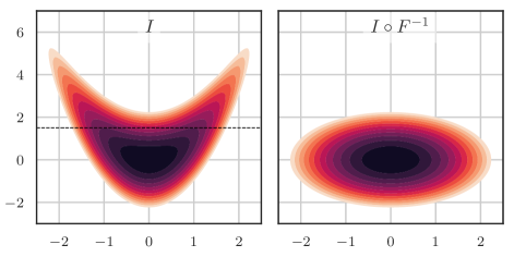
Figure 6: Left: Contour plot of the rate function (55) shows a banana-alike valley surrounding a non-convex plateau. The black dashed line represents the position of the marginal shown in figure 7. Right: The rate function composed with the inverse of the nonlinear observable (56) deforms the landscape so that the rate function becomes strictly convex.

Using this reparametrization produces a continuous and differentiable CGF of the observable $F$, resulting from the LF transform of $I\circ F^{-1}\left(y\right)$,

$$\begin{split}G_{F}\left(\lambda\right)&=\sup\limits_{F^{-1}\left(y\right)\in\mathds{R}^{2}}\left(\left\langle\lambda,y\right\rangle-I\circ F^{-1}\left(y\right)\right),\\ &=\frac{1}{4}\,\left(\lambda_{1}^{2}+\lambda_{2}^{2}\right),\end{split}$$ (57)

which allows Lagrange multipliers to reach any outcome $z$, in particular ones within the nonconvex region.

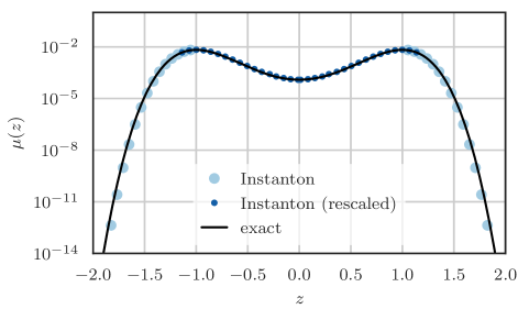
Figure 7: The marginal distribution $\mu(z)=\rho^{\infty}(z,\tfrac{3}{2})$ (as denoted by the blacked dashed line in figure 6 (left)). Instantons with linear tilt (light blue) fail to reach the region $-1<z<1$ without supporting hyperplanes of the rate function $I\left(z\right)$ (55). Performing a reparametrization using the observable (56) produces an strictly convex effective rate function ${I\circ F^{-1}\left(x\right)}$ that admits supporting hyperplanes everywhere. The corresponding instanton actions successfully capture the non-convex region (dark blue).

As numerical experiment, we choose to look at the marginal stationary distribution $\mu$ in $z_{1}$ direction for a fixed value of $z_{2}=\frac{3}{2}$, i.e. $\mu(z)=\rho^{\infty}(z,\tfrac{3}{2})$. Since at any fixed value $z_{2}>0$ we cut through the non-convex region $z_{2}>z_{1}^{2}$, the marginal distribution $\mu(z)$ looks like a double-well potential. We stress, though, that the whole system indeed has only a single fixed point. We then solve the optimization problem posed by the instanton equations with linear tilt, and compare to the minimization problem with nonlinear tilt. As shown in figure 7, the linearly tilted instanton computation produces acceptable results in the tails of the probability density (light blue dots), it fails to converge within the non-convex region $-1<z<1$: Since in that region there are no supporting planes of the rate function (55), there is no $\lambda\in\mathbb{R}^{2}$ corresponding to the slope of the supporting plane at that $z$, and consequently no tilt exists to produce the desired outcome $z$.

For the reparametrized observable (56), on the other hand, the effective rate function $I\circ F^{-1}(x)$ is convexified and admits supporting planes at every $z$. Indeed, as demonstrated in figure 7, the reparametrized optimization problem leads instanton trajectories reaching outcomes (shown as dark blue dots) within the non-convex region $-1<z<1$.

As a final remark, convexifying the rate function by the above method, even though it guarantees the existence of a tilt for every outcome, might nevertheless lead to numerical convergence issues. For example, in regions where the original rate function was convex, the rescaled optimization problem might be harder to solve, or necessitate more iterations or smaller time-steps. Similarly, even in the convexified region, the problem might become ill-posed, for example for $z_{1}\ll 1$ and $z_{2}>2$, where the observable is approximately linear.

IV.4 Nonlinear Schrödinger equation

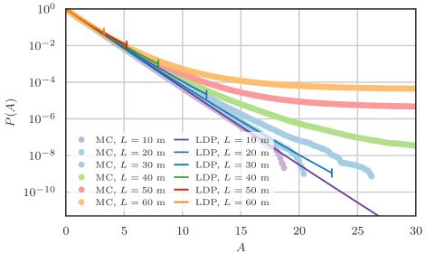
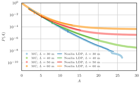
Figure 8: Left: PDF of optical power $A$ at the end of the fiber. Compared are Monte-Carlo simulations (MC, light color) with instanton prediction (dark color) for different fiber lengths, $L\in\{10\ \text{m},\dots,60\ \text{m}\}$. The tails become fatter with increasing $L$. A vertical marker is inserted at the maximal power achievable with the naive instanton method, highlighting how fat tails prevent useful instanton predictions. Right: The same, but for the instanton with nonlinear tilt, equation (71). The LDP computation now reaches far into the fat tails. The vertical markers of the naive instanton are copied over here for comparison, highlighting the increased tail reach (e.g. by more than a factor 3 for $L=60\ \text{m}$). Only lengths $L>30\ \text{m}$ are shown.

As a practical example for our proposed method, we consider the formation of extreme events in nonlinear wave equations Zakharov (1968); Osborne et al. (2000); Mori et al. (2007); Onorato et al. (2016). In the field of nonlinear optics and photonics it has been established that heavy tailed statistics frequently occur Akhmediev et al. (2013). Physical mechanisms such as soliton formation Kibler et al. (2010); Tikan et al. (2017) and nonlinear amplification Onorato et al. (2005) are responsible for the emergence of extreme power spikes out of incoherent, Gaussian initial conditions, and have been subject to investigation by a multitude of rare event algorithms Farazmand and Sapsis (2017); Dematteis et al. (2019).

Here, we consider the one-dimensional propagation of an optical pulse along a fiber, described by the nonlinear Schrödinger equation (NLS)

$$-i\partial_{x}\psi=\tfrac{1}{2}\partial_{t}^{2}\psi+|\psi|^{2}\psi\,,\quad\psi(x\!=\!0,t)=\psi_{0}(t),$$ (58)

for a complex wave envelope $\psi:[0,L]\times[0,T]\to\mathds{C}$. Boundary conditions are given at location $x=0$ at the beginning of the fiber for all times $t\in[0,T]$, and the output is measured at the end of the fiber at $x=L$. The input signal is considered random, with a Gaussian distribution of known energy spectrum. Specifically, we are mimicking an experimental setup such as Tikan et al. (2018) of a partially coherent light source, where the input signal is designed as a Gaussian shape in frequency space with covariance

$$\chi_{n}\sim\exp(-\tfrac{1}{2}\omega_{n}^{2}/\Delta\nu^{2})\,,\quad|n|<N\,,$$ (59)

with spectral bandwidth $1/\Delta\nu$ and truncation frequency $\omega_{N}$, so that the input signal is given by

$$\psi_{0}(t)=\sum_{n=-N}^{N}e^{i\omega t}\sqrt{\chi_{n}}\xi_{n}\,,$$ (60)

where $\xi_{n}$ are i.i.d. mean zero, unit variance complex Gaussian random variables.

For this setup, we are interested in the probability of measuring large spikes in the optical power $A(x,t)=|\psi(x,t)|^{2}$ at the fiber end, $x=L$. Within the presented instanton formalism, this can be achieved by tilting the distribution of initial conditions towards a high-power outcome at the fiber end, and estimating the tail probability by its most likely (“instantonic”) realization. The corresponding LDP is given by

$$p(z)=P[A(L,T/2)\geq z]\asymp\exp(-I(z))\,,$$ (61)

for a power spike of size $z$ taken arbitrarily at the center of the temporal domain, $t=T/2$. Due to the Gaussianity of the initial conditions, the rate function $I(z)$ simply is Dematteis et al. (2019)

$$I(z)=\inf_{\xi\in\mathds{C}^{2N+1}}\left(\tfrac{1}{2}|\xi|^{2}-\lambda(z)|\psi(L,T/2)|\,\right)\,.$$ (62)

Here, $\xi$ determines the source signal $\psi_{0}(t)$ through (60), while, $\lambda(z)$ can be interpreted as a Lagrange multiplier enforcing the power constraint $|\psi|^{2}=z$ at the end of the fiber. Equation (62) is therefore simply saying that the rate function is given by the most likely random configuration $\xi$ that determines a source signal with high power output. Note that, similar to the examples above, the tilt in (62) is linear, and we can therefore expect the expectation

$$\mathbb{E}\exp(-\lambda|\psi(L,T/2)|)$$ (63)

over light source signals to diverge for fiber lengths $L$ long enough for solitons to emerge and for the tails of the power distribution to become fat.

Since the probability of high power output signals at the fiber end is not known analytically, the only option we have to get comparison data is to perform Monte-Carlo (MC) simulations to sample the power distribution. To this end, we simulate the evolution of a wave packet along the fiber with a random input signals with energy spectrum (59) by numerically integrating equation (58). This equation is non-dimensionalized, with $x$, $t$ and $\psi$ normalized by characteristic parameters $\mathcal{L}_{0}$, $\mathcal{T}_{0}$ and $\mathcal{P}_{0}$ respectively, such that

$$x=\tilde{x}/\mathcal{L}_{0},\qquad t=\tilde{T}/\mathcal{T}_{0},\qquad\psi=\tilde{\psi}/\sqrt{\mathcal{P}_{0}},$$ (64)

where $\tilde{x},\,\tilde{t}$ and $\tilde{\psi}$ are the corresponding dimensional variables. These parameters $\mathcal{L}_{0}$, $\mathcal{T}_{0}$ and $\mathcal{P}_{0}$ also determine the dispersion $\beta_{2}$ and nonlinearity $\gamma$ properties of the optical fiber via

$$\beta_{2}=\mathcal{T}_{0}^{2}/\mathcal{L}_{0},\qquad\gamma=1/\left(\mathcal{L}_{0}\,\mathcal{P}_{0}\right)\,.$$ (65)

We chose these parameters according to the experimental setup in Tikan et al. (2018), where they are given as

$$\mathcal{L}_{0}=160.3\text{ m},\ \mathcal{T}_{0}=1.8778\text{ ps},\ \mathcal{P}_{0}=2.6\text{ W}\,.$$ (66)

Therefore, the optical fiber has dispersion parameter $\beta_{2}=0.022\text{ ps${}^{2}$/m}$ and nonlinearity constant $\gamma=0.0024\ (\text{Wm})^{-1}$. The spectral bandwidth $1/\Delta\nu$ is taken to be ($\Delta\nu=0.5\ \textrm{THz}$). We pick fiber lengths between $10\ \text{m}$ and $60\ \text{m}$, periodic boundary conditions in time treated pseudo-spectrally, and integrate with a second-order Runge-Kutta exponential time differencing method (ETDRK2) Du and Zhu (2005) in the spatial variable. The discretization is $\Delta x=6.24\times 10^{-3},\ \Delta t=1.3\times 10^{-2},T=106$, and frequency cut-off $N=45$. As expected, and shown in figure 8, the tails of the PDF of optical power become heavier with increasing fiber length $L$. Its samples number is $10^{6}$, where the property of $A$ being statistically homogeneous in time is used to improve the statistics.

To compare these brute-force sampling estimates to the instanton prediction, we have to solve the optimization problem (62). This is done by defining the cost functional

$$E(\xi)=\tfrac{1}{2}|\xi|^{2}-\lambda|\psi(L,T/2)|$$ (67)

for a given $\lambda$ and performing gradient descent, where the gradient is given by

$$dE/d\xi=\xi-\lambda J(L,T/2)d|\psi(L,T/2)|/d\psi\,,$$ (68)

with Jacobian $J(x,t)=d\psi(x,t)/d\xi$. This gradient can be evaluated by simultaneously integrating the NLS equation (58) and the evolution equation of the Jacobian,

$$\partial_{x}J=i\left(\tfrac{1}{2}\partial_{t}^{2}J+\psi^{2}\bar{J}+2|\psi|^{2}J\right),$$ (69)

(where $\bar{a}$ is the complex conjugate of $a\in\mathds{C}$). The iterative gradient descent algorithm yields the optimal choice $\xi^{*}$ that will lead to the desired outcome of the final power exceeding the power threshold $z$. As can be seen in figure 8 (left), the corresponding prediction for the probability, $\exp(-I(z))$ (from equation (61)) correctly describes the tail decay of high power events at the fiber end, but crucially only as long as the the rate function admits supporting lines, i.e. remains convex. Therefore, the instanton prediction is basically useless for optical fibers longer than $L=30\ \text{m}$. As a side note, the gradient computation could instead be performed in the adjoint formalism, leading to two coupled forward-backward equations similar in spirit to the instanton equations (15), but identically yielding meaningful results only in the convex region of the rate function.

Now, applying the idea from above, we can instead nonlinearly tilt the probability distribution of input signals towards high power outcomes. For this, we choose instead the nonlinearly tilted rate function

$$I(x)=\inf_{\xi\in\mathds{C}^{2N+1}}\left(\tfrac{1}{2}|\xi|^{2}-\lambda(x)F(\psi(L,T/2)\right)$$ (70)

with

$$F(z)=\log\log|z|\,,\quad|z|>1\,.$$ (71)

For this tilt, the cost functional becomes

$$E(\xi)=\tfrac{1}{2}|\xi|^{2}-\lambda F(\psi(L,T/2))$$ (72)

and the gradient is

$$dE/d\xi=\xi-\lambda J(L,T/2)dF(\psi(L,T/2))/d\psi\,,$$ (73)

instead. The results of this are shown in figure 8 (right) for the four longest fiber lengths of $30-60\ \text{m}$ in $10\ \text{m}$ increments, where the tails are fattest. In the revised formalism (dark color), the nonlinearly tilted instanton prediction is able to reach far into the stretched tail and gives the right order of magnitude for the probability of power spikes obtained from sampling (light color). The end of the region of convergence for the naive instanton is shown for comparison (vertical markers).

Note that due to the choice of reparametrization $F$ in (71), the nonlinearly tilted instanton prediction is restricted to the region of normalized power $|\psi|^{2}>1$, but of course this is exactly the tail region that we care about.

V Conclusion

Estimating the probability of tail events can efficiently be done via large deviation theory and instanton calculus, which transforms an inefficient sampling problem into a deterministic optimization problem. Unfortunately, for systems with heavy tails, or more generally non-convex rate functions, standard mechanisms of exponentially tilting the measure, or numerically solving the optimization problem, fail. The reason is the absence of a bijective map between Lagrange multiplier (tilting parameter) and desired outcome, caused by the breakdown of their Lagrange duality, or equivalently by the non-convexity of the rate function.

We put forward the idea of a nonlinear tilt that reparametrizes the output space, effectively convexifying the rate function of the observed probability distribution. We discuss the necessary conditions required for this reparametrization to yield a unique outcome variable and ensure a bijective mapping between tilt and outcome: It needs to be a diffeomorphism chosen such that its composition with the rate function is strictly convex. Note further that the reparametrization can be chosen locally, i.e. the conditions on the nonlinear observable need only apply in a subdomain of the events of interest.

Finding such nonlinear observable can be subtle, especially when the system is highly nonlinear, influencing the rate function landscape. However, drawing inspiration from toy problems with stretched exponential and algebraic tails, which can be treated analytically, yields candidate reparametrizations for physically relevant problems. We show the applicability to real-world problems by demonstrating how instantons determine the probability in extreme optical power events in a fiber optical cable, where solitons lead to a heavy-tailed power distribution at the fiber end.

VI Acknowledgement

The authors thank Eric Vanden-Eijnden for helpful discussions and Giovanni Dematteis for help with the source code for the fiber optics example. MA acknowledges the PhD funding received from UKSACB. TG acknowledges the support received from the EPSRC projects EP/T011866/1 and EP/V013319/1.

References

- Bucklew (2013) J. Bucklew, Introduction to rare event simulation (Springer Science & Business Media, 2013).
- Varadhan (1966) S. R. S. Varadhan, Communications on Pure and Applied Mathematics 19, 261 (1966).
- Dembo and Zeitouni (2010) A. Dembo and O. Zeitouni, Large deviations techniques and applications (Springer-Verlag, Berlin, 2010).
- Freidlin and Wentzell (2012) M. I. Freidlin and A. D. Wentzell, Random perturbations of dynamical systems, Vol. 260 (Springer, 2012).
- Ellis et al. (1984) R. S. Ellis et al., The Annals of Probability 12, 1 (1984).
- Deriglazov (2017) A. Deriglazov, Classical Mechanics (Springer International Publishing, Cham, 2017).
- Rindler (2018) F. Rindler, Calculus of Variations (Springer, 2018).
- Chernykh and Stepanov (2001) A. I. Chernykh and M. G. Stepanov, Physical Review E 64, 026306 (2001).
- Grafke et al. (2014) T. Grafke, R. Grauer, T. Schäfer, and E. Vanden-Eijnden, Multiscale Modeling & Simulation 12, 566 (2014).
- Grafke et al. (2013) T. Grafke, R. Grauer, and T. Schäfer, Journal of Physics A: Mathematical and Theoretical 46, 062002 (2013).
- Rolland et al. (2016) J. Rolland, F. Bouchet, and E. Simonnet, Journal of Statistical Physics 162, 277 (2016).
- Meerson et al. (2016) B. Meerson, E. Katzav, and A. Vilenkin, Physical Review Letters 116, 070601 (2016).
- Zarfaty and Meerson (2016) L. Zarfaty and B. Meerson, Journal of Statistical Mechanics-Theory and Experiment , 033304 (2016).
- Touchette (2009) H. Touchette, Physics Reports 478, 1 (2009).
- Cohen and Elliott (2015) S. N. Cohen and R. J. Elliott, Stochastic calculus and applications, Vol. 2 (Springer, 2015).
- Touchette (2005) H. Touchette, “Legendre-fenchel transforms in a nutshell,” (2005), published online: www.maths.qmul.ac.uk/~ht/archive/lfth2.pdf.
- Frisch (1995) U. Frisch, Turbulence (Cambridge University Press, Cambridge, 1995).
- Drăgulescu and Yakovenko (2001) A. Drăgulescu and V. M. Yakovenko, Physica A: Statistical Mechanics and its Applications 299, 213 (2001).
- Sinha (2006) S. Sinha, Physica A: Statistical Mechanics and its Applications 359, 555 (2006).
- Gopikrishnan et al. (2000) P. Gopikrishnan, V. Plerou, X. Gabaix, and H. E. Stanley, Physical Review E 62, R4493 (2000).
- Plerou et al. (2000) V. Plerou, P. Gopikrishnan, L. A. N. Amaral, X. Gabaix, and H. E. Stanley, Physical Review E 62, R3023 (2000).
- E et al. (2004) W. E, W. Ren, and E. Vanden-Eijnden, Communications on Pure and Applied Mathematics 57, 637 (2004).
- Grafke et al. (2017) T. Grafke, T. Schäfer, and E. Vanden-Eijnden, in Recent Progress and Modern Challenges in Applied Mathematics, Modeling and Computational Science, Fields Institute Communications (Springer, New York, NY, 2017) pp. 17–55.
- Grafke and Vanden-Eijnden (2019) T. Grafke and E. Vanden-Eijnden, Chaos: An Interdisciplinary Journal of Nonlinear Science 29, 063118 (2019).
- Zakharov (1968) V. E. Zakharov, Journal of Applied Mechanics and Technical Physics 9, 190 (1968).
- Osborne et al. (2000) A. R. Osborne, M. Onorato, and M. Serio, Physics Letters A 275, 386 (2000).
- Mori et al. (2007) N. Mori, M. Onorato, P. A. E. M. Janssen, A. R. Osborne, and M. Serio, Journal of Geophysical Research: Oceans 112, C09011 (2007).
- Onorato et al. (2016) M. Onorato, D. Proment, G. El, S. Randoux, and P. Suret, Physics Letters A 380, 3173 (2016).
- Akhmediev et al. (2013) N. Akhmediev, J. M. Dudley, D. Solli, and S. Turitsyn, Journal of Optics 15, 060201 (2013).
- Kibler et al. (2010) B. Kibler, J. Fatome, C. Finot, G. Millot, F. Dias, G. Genty, N. Akhmediev, and J. M. Dudley, Nature Physics 6, 790 (2010).
- Tikan et al. (2017) A. Tikan, C. Billet, G. El, A. Tovbis, M. Bertola, T. Sylvestre, F. Gustave, S. Randoux, G. Genty, P. Suret, et al., Physical Review Letters 119, 033901 (2017).
- Onorato et al. (2005) M. Onorato, A. R. Osborne, M. Serio, and L. Cavaleri, Physics of Fluids 17, 078101 (2005).
- Farazmand and Sapsis (2017) M. Farazmand and T. P. Sapsis, Science Advances 3, e1701533 (2017).
- Dematteis et al. (2019) G. Dematteis, T. Grafke, and E. Vanden-Eijnden, SIAM/ASA Journal on Uncertainty Quantification 7, 1029 (2019).
- Tikan et al. (2018) A. Tikan, S. Bielawski, C. Szwaj, S. Randoux, and P. Suret, Nature Photonics 12, 228 (2018).
- Du and Zhu (2005) Q. Du and W. Zhu, BIT Numerical Mathematics 45, 307 (2005).