The Large ${\color[rgb]{0,0,1}\text{N}}_{{\color[rgb]{0.75,0.0,1.0}\text{c}}}$ limit of QCD on the lattice

Abstract

We review recent progress in the study of the large $N_{c}$ limit of gauge theories from lattice simulations. The focus is not only the planar limit but also the size of ${\mathcal{O}}(N_{c}^{-1})$ corrections for values of $N_{c}\gtrsim 3$. Some concrete examples of the topics we include are tests of large-$N_{c}$ factorization, the topological susceptibility, the glueball, meson and baryon spectra, the chiral dependence of masses and decay constants, and weak matrix elements related to the $\Delta I=1/2$ rule in kaon decays.

1 Introduction

It is well known that $SU(N_{c})$ gauge theories, with and without matter content, simplify in the so called ’t Hooft or planar limit tHooft:1973alw , which corresponds to

$$N_{c}\rightarrow\infty,\;\;\;\lambda=g^{2}N_{c}={\rm fixed},$$ (1)

where $g$ is the standard gauge coupling. This limit is non-trivial, as can be expected from the fact that asymptotic freedom survives. This may be seen in the running of the ’t Hooft coupling,

$$\mu{d\lambda\over d\mu}=-{11\over 3}{\lambda^{2}\over 8\pi^{2}}+{\mathcal{O}}(\lambda^{3}),$$ (2)

which implies that a non-perturbative scale, $\Lambda^{\infty}_{\rm QCD}$, will be generated dynamically. The growth of the coupling at low energies results in charge confinement and spontaneous chiral symmetry breaking. The ’t Hooft limit therefore captures the most important non-perturbative phenomena of QCD.

In spite of the increased number of degrees of freedom, the theory simplifies to the extent that precise non-perturbative predictions can be made. In fact, it has been a long-term aspiration that the theory could be solved in this limit. An example of the simplification of the large $N_{c}$ limit is the remarkable Eguchi-Kawai (EK) reduction Eguchi:1982nm , which shows that finite volume effects are absent. Under certain conditions, the $SU(\infty)$ Yang-Mills theory can even be reduced to a matrix model on a single site. Even though the planar limit of QCD has not been solved analytically, it is unquestionable that the large $N_{c}$ limit has been of great importance in the understanding of QCD, both from a theoretical as well as phenomenological viewpoint.

Perturbative arguments indicate that the planar limit of QCD is a theory of free and infinitely narrow glueballs and hadrons tHooft:1973alw ; Witten:1979kh ; Coleman:1980nk . The hope is that the spectrum of planar QCD provides a good approximation to that at $N_{c}=3$. The description of interactions and decays requires however non-vanishing $1/N_{c}$ corrections. On the other hand, some of the planar predictions are known to fail dramatically, such as the famous $\Delta I=1/2$ rule in kaon decays, indicating the relevance of at least some of the subleading corrections. Lattice QCD can provide a quantitative, first-principles determination of the subleading ${\mathcal{O}}(1/N_{c})$ corrections to the ’t Hooft limit by directly simulating gauge theories at different $N_{c}$Teper:1998te . The strict planar limit can be most efficiently explored by numerical methods using the celebrated EK reduction and its variants. Progress in this area has been recently reviewed in GarciaPerez:2020gnf .

In this review, we will concentrate on the recent lattice explorations of $SU(N_{c})$ gauge theories with varying number of colours at zero temperature. We refer to earlier reviews on the subject Panero:2012qx ; Lucini:2012gg ; Lucini:2014bwa for further results. Although our focus will be QCD, some of the computations reviewed might be interesting in the context of compositeness models of electroweak symmetry breaking DeGrand:2019vbx ; Drach:2020qpj and dark matter models Kribs:2016cew .

The structure of the review is as follows. In sec. 2, we review the main large $N_{c}$ predictions that have been tested on the lattice. In sec. 3, we discuss the lattice approaches to the planar limit and the important issue of scale setting in this context. The main results in Yang-Mills at varying $N_{c}$ are described in sec. 4, while hadronic observables are discussed in sec. 5. We end with some concluding remarks.

2 Non-perturbative predictions at large $N_{c}$

In the absence of an analytical solution to the planar limit of Yang-Mills theories, the known predictions are based on counting powers of $N_{c}$ in perturbation theory tHooft:1973alw . A quark or antiquark is in the $N_{c}$ or $\overline{N}_{c}$ representation of $SU(N_{c})$ and has one colour index, it is therefore represented by a single directed line. A gluon is in the adjoint representation, which can be constructed out of the product of an $N_{c}$ and an $\overline{N}_{c}$, and can therefore be conveniently represented as a double line with opposite directions. The usual Feynman notation for gluons is translated to the ’t Hooft notation as depicted in Fig. 1. It is easy to see that planar vacuum diagrams involving only gluons scale as $N_{c}^{2}$ to all orders in the loop expansion, while diagrams with one fermion loop at the boundary and any internal planar exchange of gluons scale as $N_{c}$. This result can be derived, noting that a generic Feynman diagram in the double-line notation looks like polygons attached by the double lines to patch a surface. For planar diagrams the surface has the topology of a sphere, while non-planar diagrams contain handles, and fermion loops add holes. The power counting in $N_{c}$ can be shown to be related to the topology of the surface, more concretely to its Euler character, $\chi$. A diagram with $h$ handles and $f$ holes scales as

$$N_{c}^{\chi}=N_{c}^{2-2h-f}.$$ (3)

The first prediction of the large $N_{c}$ limit is that, if the theory is confining, it must be a non-interacting theory with an infinite tower of stable particles Witten:1979kh ; Coleman:1980nk . To see this, let us consider a singlet gluonic operator such as

$$O_{G}(x)={1\over N_{c}}{\rm Tr}[F_{\mu\nu}^{2}].$$ (4)

Diagrammatically, the planar contributions to the connected $n$-point correlation function scale as

$$\langle O_{G}(x_{1})...O_{G}(x_{n})\rangle_{c} \sim N_{c}^{2-n}.$$ (5)

Let us assume that there is a pole in the two point function, that is a particle in the spectrum, $|p\rangle$, the scaling of the two-point function implies

$$\langle 0|O_{G}(x)|p\rangle\sim N_{c}^{0},$$ (6)

and consequently the decay amplitude, that can be obtained from the three-point function, is suppressed by $N_{c}^{-1}$, while the scattering amplitude $2\rightarrow 2$ from the four-point function is suppressed by $N_{c}^{-2}$. The particle does not decay nor scatter as $N_{c}\rightarrow\infty$.

In addition, the number of one particle states cannot be finite, because this would imply that the large momentum behaviour of the two point function

$$\int d^{4}xe^{-ipx}\langle O_{G}(x)O_{G}(0)\rangle_{c}=\sum_{i}{g_{i}^{2}\over p^{2}+m_{i}^{2}}\sim{\mathcal{O}}(p^{-2}),$$ (7)

while asymptotic freedom predicts powers of $\log(p^{2}/m_{i}^{2})$. This can only happen if the sum over the spectrum contains an infinite number of states.

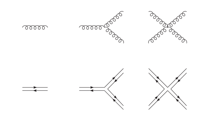
Figure 1: ’t Hooft double-line notation.

2.1 Mesons

A similar analysis can be done for mesons. Considering an operator with the quantum numbers of a meson

$$O_{M}^{a}(x)={1\over\sqrt{N_{c}}}\bar{\psi}(x)T^{a}\Gamma\psi(x),$$ (8)

the large $N_{c}$ counting gives

$$\langle O_{M}(x_{1})...O_{M}(x_{n})\rangle_{c}\sim N_{c}^{1-{n\over 2}},$$ (9)

and therefore, if there are mesonic states in the spectrum, they are stable and non-interacting in the ’t Hooft limit. The operator $O_{M}$ creates a meson from the vacuum with amplitude $N_{c}^{0}$, while the connected three-point function scales as $\sim 1/\sqrt{N_{c}}$, and the four-point function like $\sim N_{c}^{-1}$. The tower of resonances must also be infinite for the same argument outlined before for the gluons.

From eqs. (8) and (9), it follows

$$F^{2}_{\pi} \propto\langle A_{\mu}^{a}(x)A_{\mu}^{a}(y)\rangle\propto N_{c},\;\;\$$

$$\Sigma =-\langle\bar{\psi}(x)\psi(x)\rangle\ \propto N_{c},$$ (10)

while the scattering length

$$a_{M} \propto {|\langle O_{M}^{1}O_{M}^{2}O_{M}^{3}O_{M}^{4}\rangle_{c}|\over|\langle 0|O_{M}|M\rangle|^{4}}\propto N_{c}^{-1}.$$ (11)

2.2 Chiral Perturbation Theory

Spontaneous chiral symmetry breaking survives in the ’t Hooft limit Coleman:1980mx , and therefore the lightest states in the spectrum are the light pseudoscalar mesons. Their mass is ${\mathcal{O}}(N_{c}^{0})$, assuming the quark mass does not scale with $N_{c}$, since to leading order in the quark mass:

$$M^{2}_{\pi}={\Sigma\over F_{\pi}^{2}}(m_{u}+m_{d}).$$ (12)

Chiral perturbation theory (ChPT) and the chiral Lagrangian Gasser:1984gg describe accurately meson interactions at low energies as an expansion in momentum and quark mass:

$${\mathcal{L}}_{\chi}={\mathcal{L}}^{(2)}_{\chi}+{\mathcal{L}}^{(4)}_{\chi}+...,$$ (13)

with

$${\mathcal{L}}^{(2)}_{\chi} = {F^{2}\over 4}{\rm Tr}[\partial_{\mu}U^{\dagger}\partial^{\mu}U]-{\Sigma\over 2}{\rm Tr}[M_{q}U+h.c.],$$

$${\mathcal{L}}^{(4)}_{\chi} = \sum_{i=1,10}L_{i}{\mathcal{O}}_{i}[U,\partial_{\mu},M_{q}],$$ (14)

where $M_{q}$ is the quark mass matrix, $U=\exp(i{\sqrt{2}\pi\over F})$ and $\pi$ represents the pions, in the adjoint representation of $SU(N_{f})$. The operators ${\mathcal{O}}_{i}$ are Lorentz and chirally invariant combinations of $U$, with four derivatives or two quark mass matrices. The $L_{i}$ are the famous low-energy couplings (LECs) Gasser:1984gg . The expansion parameter in ChPT is

$$\left(M_{\pi}\over 4\pi F_{\pi}\right)^{2}\sim\left(p\over 4\pi F_{\pi}\right)^{2}\sim{1\over N_{c}},$$ (15)

and becomes smaller and smaller as $N_{c}\rightarrow\infty$. However, the range of validity to the chiral effective theory does not increase: the failure of the chiral expansion will be abrupt when the energy reaches the mass of the heavy resonances, $\Lambda_{\chi}$. These masses are expected to scale as $N_{c}^{0}$, and therefore remain constant as we approach $N_{c}\rightarrow\infty$. One may typically consider $\Lambda_{\chi}\sim M_{\rho}$.

An additional simplification of the chiral Lagrangian comes from the fact that only a subset of the low-energy couplings Gasser:1984gg are leading in $N_{c}$, ie. $L_{i}\propto{\mathcal{O}}(N_{c})$. These are the ones that correspond to chiral operators (${\mathcal{O}}_{i}$) with a single flavour trace. This is because according to the general rules, diagrams with more than one fermion loop are subleading. More concretely, for $N_{f}=3$ Gasser:1984gg ; Peris:1994dh :

$$L_{1},L_{2},L_{3},L_{5},L_{8},L_{9},L_{10} \propto {\mathcal{O}}(N_{c}),$$

$$2L_{1}-L_{2},L_{4},L_{6},L_{7} \propto {\mathcal{O}}(1).$$ (16)

Phenomenological approaches have estimated the leading $N_{c}$ behaviour of these couplings by assuming that the chiral theory matches onto a theory of free resonances, the resonant chiral theory Ecker:1988te . The low-energy couplings result from the exchange of heavier resonances and can be extracted in terms of the measured spectrum, and imposing the correct large momentum behaviour of certain correlation functions. For a review see Pich:2002xy .

It is well-known that the standard chiral Langrangian needs to be extended to include the $\eta^{\prime}$ DiVecchia:1980yfw ; PhysRevD.21.3388 ; Witten:1980sp ; Kawarabayashi:1980dp ; Gasser:1984gg ; Leutwyler:1996sa ; HerreraSiklody:1996pm ; Kaiser:2000gs , since the singlet meson becomes degenerate with the remaining pseudoscalar mesons in the planar limit. The $\eta^{\prime}$ mass receives a contribution from the $U_{A}(1)$ anomaly, that scales as $N_{c}^{-1}$. The Witten-Veneziano (WV) formula Witten:1979vv ; Veneziano:1979ec (see also Giusti:2001xh ; Seiler:2001je ; Giusti:2004qd ; Luscher:2004fu ; DelDebbio:2004ns ) relates this contribution with the topological susceptibility computed in a theory without quarks, ie. in Yang-Mills (YM):

$$M_{\eta^{\prime}}^{2}\equiv{2N_{f}\over F^{2}_{\pi}}\int d^{4}x\langle q(x)q(0)\rangle_{YM}\left[1+{\mathcal{O}}(N_{c}^{-1})\right],$$ (17)

where

$$q(x)\equiv{\lambda\over 32\pi^{2}N_{c}}{\rm Tr}[F_{\mu\nu}(x){\tilde{F}}^{\mu\nu}(x)],$$ (18)

and we have considered massless quarks. The topological susceptibility measures the $\theta$ dependence of the vacuum energy, which should vanish for massless quarks. The WV relation can be deduced from requiring that the $\eta^{\prime}$ contribution to the $\theta$ dependence exactly cancels the leading gluonic contribution, or from the anomalous chiral Ward identity. This is one example where the diagrammatic analysis leads to the wrong conclusion: the leading $N_{c}$ scaling of the topological susceptibility is cancelled by a naively subleading one.

The presence of the $\eta^{\prime}$ in the chiral Lagrangian makes it necessary to correlate the large $N_{c}$ and the momentum/mass expansions. The pion manifold is now $U(N_{f})$, and a consistent power counting HerreraSiklody:1996pm ; Kaiser:2000gs ensures the same scaling of the $\eta^{\prime}$ mass and the remaining pseudoscalar mesons:

$${\mathcal{O}}(M_{\pi}^{2})\sim{\mathcal{O}}(M_{\eta^{\prime}}^{2})\sim{\mathcal{O}}\left({1\over N_{c}}\right).$$ (19)

2.3 Baryons

Baryons are trickier in the ’t Hooft limit, since their mass has a non-trivial scaling. Nevertheless their properties can also be understood in a systematic expansion in $1/N_{c}$ Witten:1979kh ; Dashen:1993jt ; Jenkins:1993zu ; Carone:1993dz ; Dashen:1994qi ; Dai:1995zg . By simple arguments, it can be seen that the baryon mass scales with $N_{c}$. We recall that in QCD a colour singlet can be formed by combining three quarks in the fundamental representation: $\mathbf{3}\otimes\mathbf{3}\otimes\mathbf{3}\to\mathbf{1}$. In a general $SU(N_{c})$ theory, one would however need $N_{c}$ fundamental quarks to create a baryon. This motivates the simple expectation for the baryon mass: $M_{B}=m_{0}N_{c}+O(N_{c}^{0})$. Moreover, the baryon–baryon to n-meson amplitude scales like $\sqrt{N_{c}}^{1-n}$.

Spin-flavour symmetry results in consistency conditions that allow to understand for example the baryon hyperfine splitting Jenkins:1993zu :

$${M_{B}\over N_{c}}=m_{0}+B{J(J+1)\over N_{c}^{2}}+C\left({J(J+1)\over N_{c}^{2}}\right)^{2}+...,$$ (20)

where $J$ is the baryon spin, and $m_{0},B$ and $C$ are $O(N_{c}^{0})$ constants. For a detailed review on baryons in large $N_{c}$ see Manohar:1998xv .

2.4 Exotics

An interesting and timely question is that of exotic states, such as tetraquarks. The standard lore Witten:1979kh ; Coleman:1980nk used to be that tetraquarks cannot exist in the ’t Hooft limit. The argument however has been revised recently PhysRevLett.110.261601 ; PhysRevD.88.036016 . The most recent conclusion is that the large $N_{c}$ scaling does not allow to establish whether these particles exist or not in the spectrum, however if they do they must be infinitely narrow, just like glueballs and mesons, for the same reasons outlined above. An analysis of the expected scaling of the decay width of tetraquarks with different flavour content can be found inPhysRevD.88.036016 .

It is interesting to analyse the old argument supporting the non-existence of exotics Witten:1979kh ; Coleman:1980nk . It relies on the fact that the two point correlation function of two tetraquark operators (constructed from two quark bilinears) has a factorized contribution, leading in $N_{c}$, corresponding to the propagation of two non-interacting mesons. However, the tetraquark pole, if it exists, should appear in the connected part of the correlatorPhysRevLett.110.261601 which is subleading in $N_{c}$. In other words the factorized and connected terms might describe the dynamics of different processes, one is not necessarily the subleading $N_{c}$ correction of the other, and both can in principle survive the ’t Hooft limit. It might be a challenge in practice to isolate such exotic states from a two meson state, since the overlap of any operator with the right quantum numbers with the two meson state dominates over that with the exotic one.

2.5 Factorization

More generally, large $N_{c}$ implies the factorization of expectation values of products of singlet operators in the pure gauge theory:

$$\langle O_{1}O_{2}\rangle=\langle O_{1}\rangle\langle O_{2}\rangle\left[1+{\mathcal{O}}\left({1\over N^{2}_{c}}\right)\right].$$ (21)

This property underlies for example the OZI rule and the EK reduction. It should be stressed however that the disconnected and connected parts of any such observable could represent different physics.

2.6 Weak interactions

Finally, we discuss hadronic weak interactions in the planar limit. One of the most famous failures of the large $N_{c}$ approximation is the $\Delta I=1/2$ rule, that is the large hierarchy observed in the kaon decay amplitudes to two pions in the two possible states of isospin $I=0,2$:

$$T[K^{0}\rightarrow(\pi\pi)_{I}]=iA_{I}e^{i\delta_{I}},\;\;\;\;\left|{A_{0}\over A_{2}}\right|\sim 22.$$ (22)

These amplitudes were established as benchmark lattice calculations since the early days Brower:1984ta , but remain very challenging. Only very recentlyBoyle:2012ys ; Bai:2015nea ; Blum:2015ywa ; Ishizuka:2018qbn ; Abbott:2020hxn , convincing evidence has been presented that the $\Delta I=1/2$ rule is reproduced near the physical point of $2+1$ simulations. It is well known that the $\Delta I=1/2$ rule plays a key role in the Standard Model prediction of the direct CP violating ratio $\epsilon^{\prime}/\epsilon$.

Surprisingly large $N_{c}$ misses completely the $\Delta I=1/2$ enhancement Fukugita:1977df ; Chivukula:1986du . This is easy to see by comparing the large $N_{c}$ scaling of the decays $K^{+}\rightarrow\pi^{+}\pi^{0}$ and $K^{0}\rightarrow\pi^{0}\pi^{0}$, which in terms of the isospin amplitudes are:

$$-iT[K^{0}\rightarrow\pi^{0}\pi^{0}] = \sqrt{2\over 3}A_{2}e^{i\delta_{2}}-{1\over\sqrt{3}}A_{0}e^{i\delta_{0}}\propto{\mathcal{O}}(N_{c}^{-{1\over 2}}),$$

$$-iT[K^{+}\rightarrow\pi^{+}\pi^{0}] = {\sqrt{3}\over 2}A_{2}e^{i\delta_{2}}\propto{\mathcal{O}}(N_{c}^{1\over 2}),$$ (23)

where the $N_{c}$ scaling can be easily deduced by inspection of the diagrams, see Fig. 2, contributing to each amplitude. This implies that, at the leading order in large $N_{c}$, the neutral $K^{0}$ does not decay and therefore from eq. (23) it follows:

$$\left|{A_{0}\over A_{2}}\right|_{N_{c}\rightarrow\infty}=\sqrt{2}.$$ (24)

One possible explanation of this discrepancy is the fact that the dynamics involves multiple scales: the $W$ mass, the charm mass and hadronic scales, and maybe subleading $1/N_{c}$ corrections could be enhanced by large logarithms.

$$\begin{array}[]{cc}\raisebox{-0.45pt}{\includegraphics[scale={1}]{plots/Ktopipicharged.pdf}}&\hskip 8.5359pt{\mathcal{O}\Big{(}N_{c}^{1/2}\Big{)}}\\ \\ \raisebox{-0.43pt}{\includegraphics[scale={1}]{plots/Ktopipineutral.pdf}}&\hskip 8.5359pt{\mathcal{O}}\Big{(}N_{c}^{-1/2}\Big{)}\\ \end{array}$$

Figure 2: Leading diagrams in the $N_{c}$ scaling of $K^{+}\to\pi^{+}\pi^{0}$ (top), and $K^{0}\to\pi^{0}\pi^{0}$ (bottom).

At energies below the $W$-boson mass, we can integrate it out and represent the weak interactions in the Fermi theory. For example the CP-conserving $\Delta S=1$ transitions the Hamiltonian density takes the simple form:

$${\mathcal{H}}^{N_{f}=4}_{\Delta S=1}=\sqrt{2}G_{\rm F}V_{us}^{*}V_{ud}(k^{+}\,\bar{Q}^{+}(x)+k^{-}\,\bar{Q}^{-}(x))\,,$$ (25)

with $\bar{Q}^{\pm}=Z_{Q}^{\pm}Q^{\pm}$ and

$$Q^{\pm}= (\bar{s}_{L}\gamma_{\mu}u_{L})(\bar{u}_{L}\gamma^{\mu}d_{L})\pm(\bar{s}_{L}\gamma_{\mu}d_{L})(\bar{u}_{L}\gamma^{\mu}u_{L})$$ (26)

$$-[u\leftrightarrow c].$$

We have neglected quark masses and included all the operators compatible with the ${\rm SU}(4)_{\rm L}\times{\rm SU}(4)_{\rm R}$ flavour symmetries. $Q^{+}$ transforms as the $(84,1)$, while $Q^{-}$ transforms as the $(20,1)$. Only $\bar{Q}^{+}$ contributes to the $A_{2}$ amplitude, and therefore a hierarchy in the matrix elements of the two operators is needed to explain the rule. This effective Hamiltonian should be valid down to energies above the charm mass. The Wilson coefficients $k^{\pm}$ do indeed get large logarithms from the $M_{W}\rightarrow\mu$ Gaillard:1974nj ; Altarelli:1974exa , but it is not enough to explain the large hierarchy, since $k^{-}(m_{c})/k^{+}(m_{c})\sim 2$.

Below the charm threshold the theory matches onto the $N_{f}=3$ theory, that has the form Buchalla:1995vs

$${\mathcal{H}}^{N_{f}=3}_{\Delta S=1}=\sqrt{2}G_{\rm F}V_{us}^{*}V_{ud}\sum_{\sigma=1,...6}k_{\sigma}Q_{\sigma},$$ (27)

where the operators in the list include all operators that transform as $(27,1)$ or $(8,1)$, ignoring QED effects. Among the latter, we find the famous penguin operators such as

$$Q_{6}=(\bar{s}_{L}\gamma_{\mu}d_{L})\sum_{q=u,d,s}(\bar{q}_{R}\gamma^{\mu}q_{R}).$$ (28)

The standard lore for a long time was that the matrix elements of the penguin operators were enhanced and, since they are octets that do not contribute to $A_{2}$, this fact could be at the origin of the $\Delta I=1/2$ Vainshtein:1976nd . This hypothesis does not seem to be confirmed by the last lattice results, where the current operators of eq. (26) give the dominant contribution to the real part of the isospin amplitudes, as anticipated long ago in Ref. Bardeen:1986uz . Instead it has been argued that the enhancement originates in a strong cancellation of the colour-connected and colour-disconnected contributions of the current operator matrix elements Boyle:2012ys . Such contributions have a different $N_{c}$ scaling, and therefore indicate anomalously large $N_{c}$ corrections.

At sufficiently low energies and quark masses, a further simplification is possible since the effective hamiltonians, eqs. (25) or (27) can be matched to the corresponding $N_{f}=4$ (if the charm is considered light) or $N_{f}=3$ (for a heavy charm) chiral effective theories. At the leading order of the chiral expansion, the structure of the chiral weak hamiltonian in the $N_{f}=4$ theory is Giusti:2004an ; Giusti:2006mh

$${\mathcal{H}}^{N_{f}=4}_{\rm ChPT}=\sqrt{2}G_{\rm F}V_{us}^{*}V_{ud}(g^{+}\,{\mathcal{Q}}^{+}+g^{-}\,{\mathcal{Q}}^{-})\,,$$ (29)

with

$${\mathcal{Q}}^{\pm} = {F_{\pi}^{4}\over 4}\left[(U\partial_{\mu}U^{\dagger})_{us}(U\partial_{\mu}U^{\dagger})_{du}\pm(U\partial_{\mu}U^{\dagger})_{ds}(U\partial_{\mu}U^{\dagger})_{uu}\right.$$ (30)

$$- \left.(u\rightarrow c)\right].$$

It is straightforward to evaluate the ratio of amplitudes in terms of the low-energy couplings $g^{\pm}$ to lowest order in ChPT:

$${A_{0}\over A_{2}}={1\over 2\sqrt{2}}\left(1+3{g^{-}\over g^{+}}\right).$$ (31)

A large ratio $g^{-}/g^{+}$ could explain the $\Delta I=1/2$ rule, an effect that would be unrelated to the charm threshold.

These low-energy couplings can be determined from matching appropriate correlation functions in ChPT and lattice QCDGiusti:2004an ; Giusti:2006mh . The simplest choices are the ratios:

$$R^{\pm}=\kern-10.00002pt\lim_{\begin{subarray}{c}z_{0}-x_{0}\to\infty\\ y_{0}-z_{0}\to\infty\end{subarray}}\frac{\sum_{{\mathbf{x}},{\mathbf{y}}}\langle P(y)Q^{\sigma}(z)P(x)\rangle}{\sum_{{\mathbf{x},\mathbf{y}}}\langle P(y)A_{0}(z)\rangle\langle P(x)A_{0}(z)\rangle},$$ (32)

with $A_{0}(x)\equiv\bar{\psi}^{i}(x)\gamma_{0}\gamma_{5}\psi^{j}(x)$ and $P(x)=\bar{\psi}^{i}(x)\gamma_{5}\psi^{j}(x)$, with appropriately chosen flavours $i,j$.

Including the renormalization factors and the Wilson coefficients, we get the physical amplitudes, $A^{\pm}$, that can be matched to the corresponding observables in the chiral theoryGiusti:2004an ; Giusti:2006mh . At lowest order the matching condition is

$$\lim_{M_{\pi}\rightarrow 0}A^{\pm}=g^{\pm}.$$ (33)

The $\pm$ three-point functions are the sum of a colour-disconnected diagram and a colour-connected one, that scale differently with $N_{c}$ , see Fig. 3. The relative sign is $\mp$ in the $A^{\pm}$ amplitudes.

$$\begin{array}[]{lll}\raisebox{-0.5pt}{\includegraphics[scale={0.8}]{plots/dis.pdf}}&\mp&\raisebox{-0.5pt}{\includegraphics[scale={0.8}]{plots/con.pdf}}\\ \end{array}$$

Figure 3: Colour-disconnected (left) and colour-connected (right) contributions to the three-point function in $R^{\pm}$.

The standard diagrammatic $N_{c}$ counting results in the following scaling:

$$A^{\pm}=1\pm\tilde{a}{1\over N_{c}}\pm\tilde{b}{N_{f}\over N^{2}_{c}}+\tilde{c}{1\over N^{2}_{c}}+\tilde{d}{N_{f}\over N^{3}_{c}}+\cdots,$$ (34)

where the coefficients $\tilde{a}-\tilde{d}$ are independent of $N_{c}$ and $N_{f}$, and a natural expectation is that they are ${\mathcal{O}}(1)$. Diagrams contributing to ${\tilde{c}}$ and ${\tilde{d}}$ are shown in Fig. 5 while those contributing to $\tilde{a}$ and $\tilde{b}$ are in Fig. 5.

$$\begin{array}[]{ccc}{\tilde{c}}:&\raisebox{-0.5pt}{\includegraphics[scale={0.7}]{plots/disnlo.pdf}}&{\mathcal{O}}(N_{c}^{0})\\ {\tilde{d}}:&\raisebox{-0.5pt}{\includegraphics[scale={0.7}]{plots/disnlonf.pdf}}&{\mathcal{O}}\left({N_{f}\over N_{c}}\right)\\ \end{array}$$

Figure 4: $N_{c},N_{f}$ scaling of various contributions to the colour-disconnected contraction of the three-point function.

$$\begin{array}[]{ccc}\tilde{a}:&\raisebox{-0.5pt}{\includegraphics[scale={0.7}]{plots/conlo2.pdf}}&{\mathcal{O}}(N_{c})\\ \tilde{b}:&\raisebox{-0.5pt}{\includegraphics[scale={0.7}]{plots/connlonf.pdf}}&\mathcal{O}\left(N_{f}\right)\\ \end{array}$$

Figure 5: $N_{c},N_{f}$ scaling of various contributions to the colour-connected contraction of the three-point function.

We find that the leading correction, ${\mathcal{O}}(1/N_{c})$ together with the leading effects of dynamical quarks, ${\mathcal{O}}(N_{f}/N_{c}^{2})$, are fully anticorrelated in the ratios. This analysis does not predict the sign of the different terms, i.e., the sign of the $\tilde{a}-\tilde{d}$ coefficients, only the (anti)-correlation between the two amplitudes. In particular, a negative sign of $\tilde{a}$ and $\tilde{b}$ results in an enhancement of the ratio $A^{-}/A^{+}$. The scaling of eq. (34) is valid for all quark masses, but the different coefficients could be have a different quark mass dependence.

The lattice can in principle measure all these coefficients and determine whether they have the natural size, ${\mathcal{O}}(1)$, and quantify to what extent the anti-correlation is enough to explain the $\Delta I=1/2$ rule.

A similar matching to chiral perturbation theory could also be done in the $N_{f}=3$ flavour theory, where the leading order weak Hamiltonian has also two operators with the same chiral structure, corresponding to the $27$-plet and octet operatorsBernard:1985wf . The case of a heavy charm is however much more demanding, not only the list of operators to consider on the lattice is much longer, but it involves the computation of all-to-all propagators.

There is a long list of phenomenological analyses that have used large-$N_{c}$ inspired methods to estimate the size of these couplings, in an analogous way to the strong couplings, $L_{i}$. Examples are the dual QCD approach Bardeen:1986vp ; Bardeen:1986uz ; Buras:2014maa , the resonance chiral theory Ecker:1988te or the chiral quark model Antonelli:1995nv , etc. In all cases, the relevance of subleading corrections in $N_{c}^{-1}$ has been demonstrated, and argued to be related to a strong scale dependence. Incorporating these systematically is not easy and the error resulting from these approaches is therefore quite uncertain. For a review see Cirigliano:2011ny .

3 Lattice QCD at large $N_{c}$

Two approaches have been followed to explore the ’t Hooft limit in the lattice formulation. The most straightforward approach is to simulate at different values of $N_{c}$ Teper:1998te ; Lucini:2001ej ; Lucini:2003zr ; Lucini:2008vi , and study the scaling of any physical quantity in units of some reference scale, such as $\Lambda_{QCD}$, which is well defined when $N_{c}\rightarrow\infty$. The cost of the simulation increases with $N_{c}$, in particular, for dynamical simulations the cost of a single configuration scales like $\sim N_{c}^{2}$, dominated by matrix-vector multiplications for the inversion of the Dirac operator. However, statistical fluctuations seem to decrease, as can be expected from the factorization property, eq. (21). This was also observed in Refs. Hernandez:2019qed ; Donini:2020qfu , although a large $N_{c}$ scaling of the autocorrelation time has not been done yet. Reaching very large values of $N_{c}={\mathcal{O}}(100)$ is however not possible with this method. The Eguchi-Kawai reductionEguchi:1982nm allows to study the leading behaviour in $N_{c}$ much more efficiently by exploiting the volume independence ensured by factorization, and reducing the model to a single-point lattice model. Different variants of the EK reduction exist BHANOT198247 ; Narayanan:2003fc ; Kovtun:2007py ; Unsal:2008ch ; GONZALEZARROYO1983174 ; PhysRevD.27.2397 in the literature, and they have been successfully implemented to compute the ’t Hooft limit of several physical observables Gonzalez-Arroyo:2014dua ; GONZALEZARROYO1983415 ; FABRICIUS1984293 ; GonzalezArroyo:2012fx ; Gonzalez-Arroyo:2015bya ; Hietanen:2009tu . We will show some of the most recent results, but a more detail account of reduced models can be found in GarciaPerez:2020gnf .

The complementarity of both approaches is evident when trying to evaluate the subleading $1/N_{c}$ corrections. While these corrections cannot be captured by the reduced models, they can be straightforwardly computed with the direct method. The input provided by the reduced model on the planar limit is nevertheless very helpful to constrain the asymptotic $N_{c}$ dependence.

3.1 Scale setting and $N_{c}$-dependence

The outcome of a lattice calculation is always a either dimensionless ratio, or a dimensionful quantity in terms of the lattice spacing, $a$. In QCD, the value of the lattice spacing is typically fixed by some experimental input (e.g., a mass or decay constant). Once $a$ is known, any observable can be converted to physical units (MeV, fm,…). The procedure of computing $a$ in physical units is known as the (absolute) scale setting. Of course, a complete calculation will require simulations at multiple values of $a$, and a continuum limit extrapolation for the observables of interest.

In the context of large $N_{c}$, the scale setting is a more subtle issue, and it necessarily involves some arbitrariness. To illustrate this, let us consider the case of a pure $SU(N_{c})$ gauge theory. We could perform simulations with varying $N_{c}$, and compute the ratio of two different scales, $\Lambda_{1}/\Lambda_{2}$ in the continuum limit. These scales could for instance be masses of glueballs with different quantum numbers. Then, we could fit the functional form of the $N_{c}$-dependence as:

$$\frac{\Lambda_{2}}{\Lambda_{1}}=c_{1}+\frac{c_{2}}{N_{c}^{2}}+\ldots,$$ (35)

in the pure gauge theory without fermions. This is a well-posed problem, and does not require any absolute knowledge of the lattice spacing (only a relative one for the continuum limit). We may however know the value for these two scales from experiments in QCD, and we would like to infer their values as a function of $N_{c}$. For this, one necessarily needs to impose a known $N_{c}$ dependence—an all-orders ansatz—for one of the scales of the theory. The simplest choice is to pick, e.g., $\Lambda_{1}$ as constant for all values of $N_{c}$. This fully fixes the prescription for the large $N_{c}$ limit, and implicitly the lattice spacing at all values of $N_{c}$ via the scale $\Lambda_{1}$. It is clear that different choices of $\Lambda_{1}$ will produce differences in the subleading $1/N_{c}$ corrections for other physical quantities, but the same ratios in two different prescriptions will have the same $N_{c}$ scaling.

From a practical point of view, it is much more convenient to study the $N_{c}$ dependence by using lattice simulations at a constant line of physics. In other words, to establish the prescription for the large $N_{c}$ limit at the time of the simulation. For instance, in early work Lucini:2001ej , simulations were compared at a constant value of the mean-field improved bare ’t Hooft coupling defined as:

$$\lambda_{I}(a^{-1})=\frac{2N_{c}^{2}}{\beta P},$$ (36)

where $P$ is the plaquette normalized by $N_{c}$. One may say that simulations with constant $\lambda_{I}$ at different $N_{c}$ have the same value of the lattice spacing. Thus, after fixing $a$ from $N_{c}=3$, the large $N_{c}$ prescription is fully fixed.

A different line of constant physics was chosen in Ref. Bali:2013kia . There, the string tension —labelled as $\sigma$—was used. In this work, the authors used existing results for $\sigma$ as a function of $N_{c}$ DelDebbio:2001sj ; Lucini:2005vg ; Allton:2008ty ; Lucini:2012wq ; Lohmayer:2012ue to generate gauge configurations with $N_{c}\in[2,17]$ and fixed value of $a\sqrt{\sigma}$. Moreover, they used the “ad hoc value $\sigma=1$ GeV/fm” to define their lattice spacing for all values of $N_{c}$. To further iIlustrate the ambiguity at large $N_{c}$, we can look at the behaviour of the coupling in eq. (36) in the simulations in Ref. Bali:2013kia . We will easily see that $\lambda_{I}(a^{-1})$ it is not constant, but rather it is modified at order $1/N_{c}^{2}$.

In the last few years, the usage of the gradient flow Luscher:2010iy has become customary for the scale setting on the lattice Sommer:2014mea —also in the context of large $N_{c}$. The advantage is that the energy density can be used to determine a renormalized ’t Hooft coupling in the gradient flow scheme:

$$\langle E(t)\rangle\equiv\frac{1}{4}\langle G_{\mu\nu}^{a}G^{\mu\nu}_{a}\rangle=\frac{3}{138\pi^{2}t^{2}}\frac{N_{c}^{2}-1}{N_{c}}\lambda_{GF},$$ (37)

with $\lambda_{GF}$ defined at the scale $1/\sqrt{8t}$. The gradient flow coupling has been related to the $\overline{MS}$ coupling in perturbation theory Harlander:2016vzb . A standard approach in QCD is to define the scale $t_{0}$ via the energy density as a function of the flow time:

$$t^{2}\langle E(t)\rangle\big{\rvert}_{t=t_{0}}=0.3.$$ (38)

Even though $t_{0}$ cannot be measured experimentally, its value in physical units has been extracted from various lattice calculations Bruno:2013gha ; Sommer:2014mea ; Bruno:2016plf . In Ref. Ce:2016awn it was proposed to generalize the definition of $t_{0}$ to

$$t^{2}\langle E(t)\rangle\big{\rvert}_{t=t_{0}}=0.3\times\frac{3}{8}\frac{N_{c}^{2}-1}{N_{c}},$$ (39)

so that results at different $N_{c}$ may be compared. Moreover, the same authors opt for fixing $\sqrt{t_{0}}\sim 0.166$ fm for all values of $N_{c}$.

In dynamical simulations with varying $N_{c}$, an additional convention regarding the quark mass must be imposed to compare across values of $N_{c}$. This is because a generic observable, including $t_{0}$, depends on the quark masses. An option that fully fixes the convention could be matching the chirally extrapolated value of $t_{0}$ for different gauge groups. In Ref. DeGrand:2017gbi with $N_{f}=2$ simulations, two different conditions were imposed: (i) the ratio $\sqrt{t^{\prime}_{0}}/r_{1}$ is fixed, where $t^{\prime}_{0}$ for $N_{c}=3$ is the standard one in eq. (38), and $r_{1}$ is related to the Sommer parameter Sommer:1993ce ; Bernard:2000gd , and (ii) the ratio of the vector meson mass over the pion mass is matched. More recently, in Ref. Hernandez:2019qed with $N_{f}=4$ simulations, the generalized value of $t_{0}$ as in eq. (39) at $M_{\pi}=420$ MeV was fixed for all values of $N_{c}$.

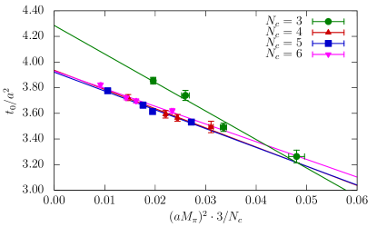
Figure 6: Chiral dependence of $t_{0}$ for various simulations with $N_{f}=4$ and $N_{c}=3-6$. Source: Ref. Hernandez:2019qed .

As a further check of the consistency of this scale setting, one can also study the chiral dependence of $t_{0}$ when varying the number of colours. The prediction from Chiral Perturbation Theory is Bar:2013ora :

$$t_{0}(M_{\pi})=t_{0}^{\chi}\left(1+\frac{k}{N_{c}}M_{\pi}^{2}\right)+O(M_{\pi}^{4}),$$ (40)

with $t_{0}^{\chi},k$ being low-energy constants. We note that the $1/N_{c}$ suppression of the mass dependence is consistent with the quenched limit, in which $t_{0}$ is mass independent. In Fig. 6, we show this chiral dependence along with the corresponding chiral fits. As can be seen, the data for $N_{c}=4,5,6$ lie almost on top of some universal line, whereas $N_{c}=3$ has larger $1/N_{c}$ effects.

4 Yang-Mills theories at large $N_{c}$

In this section, we review various results for pure $SU(N_{c})$ Yang-Mills theories, including the factorization theorem, the glueball spectrum and topological observables.

4.1 Large $N_{c}$ factorization

One of the simplest yet powerful results in the large $N_{c}$ limit is the factorization of observables, eq. (21). This result is derived from a perturbative analysis, but can be tested non perturbatively in lattice simulations at different values of $N_{c}$. Recently, such study was carried out in Refs. Vera:2018lnx ; GarciaVera:2017xif .

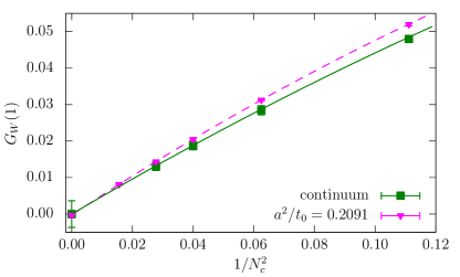
Figure 7: Large $N_{c}$ extrapolations of $G_{W}(1)$ in the continuum (solid line) and at finite lattice spacing (dashed line). Source: Ref. Vera:2018lnx .

In order to test the factorization hypothesis, the authors use various quantities, e.g., a square spatial Wilson loop at the point $(x_{0},{\mathbf{x}})$ with size $R_{c}$ and Wilson-flowed to time $t$:

$$\begin{split}W(c)&=\langle W(t,x_{0},\vec{x},R_{c})\rangle,\\ W^{sq}(c)&=\langle W^{2}(t,x_{0},\vec{x},R_{c})\rangle,\end{split}$$ (41)

The flow time is a fraction of $t_{0}$, eq. (39), $t=ct_{0}$, and the size is chosen as $R_{c}=\sqrt{8ct_{0}}$. Note that the authors use open boundary conditions, to avoid topology freezing, and $x_{0}$ must be taken far from the boundary. The ratio

$$G_{W}(c)=\frac{W^{sq}(c)-W^{2}(c)}{W^{2}(c)},$$ (42)

according to the factorization property, is expected to be of order $1/N_{c}^{2}$. The results for $G_{W}(1)$ in this study are shown in Fig. 7. As can be seen, the authors find very good consistency with the factorization hypothesis both at a finite lattice spacing (fixed $t_{0}/a^{2}$), and in the continuum limit. For other gluonic observables, the authors also find the expected large $N_{c}$ scaling and confirm the factorization hypothesis.

The dependence of $G_{W}(c)$ on the size of the loop is also studied. For this, they define a new observable $\hat{G}_{W}(\xi)$, that depends on the Wilson loop

$$\widehat{W}(\xi)=\langle W(t_{0}/2,x_{0},\vec{x},R_{\xi})\rangle$$ (43)

with varying radius, $R_{\xi}=\xi\sqrt{4t_{0}}$. The authors fit the $1/N_{c}$ scaling as:

$$\widehat{G}_{W}(\xi)=b_{0}+b_{1}\frac{1}{N_{c}^{2}}+b_{2}\frac{1}{N_{c}^{4}}.$$ (44)

As expected, $b_{0}$ is always compatible with zero. In contrast, the results for the coefficient of the subleading corrections , shown in Fig. 8, seem to grow exponentially with the size of the Wilson loop.

This shows that the coefficient of the subleading corrections can be large, but this is not necessarily a signal of failure of the large $N_{c}$ expansion. This is because the leading and subleading contributions can be related to different physics scales. While the disconnected and leading term is controlled by the static potential, the connected part could get contributions from other physics scales.

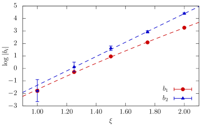
Figure 8: Dependence of the corrections to factorization with the size of the Wilson loop, $\xi$ [see eq. (43)]. The $b_{i}$ parameters are those of eq. (44). For each parameter, we include a quadratic interpolating line. Source: Ref. Vera:2018lnx .

4.2 Glueballs at large $N_{c}$

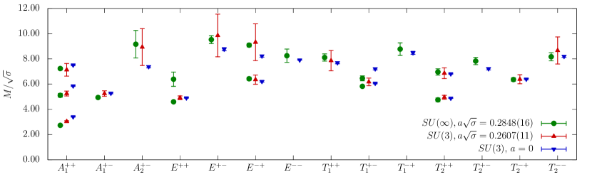
Figure 9: Spectrum of glueballs at finite lattice spacing in the large $N_{c}$, and $N_{c}=3$ from Ref. Lucini:2010nv . Some of the $SU(3)$ levels were not determined in Ref. Lucini:2010nv . As a comparison, we also include the continuum limit results for $SU(3)$ from Ref. Athenodorou:2020ani .

The glueball spectrum is a very interesting nontrivial manifestation of non perturbative dynamics in the pure Yang-Mills theory. Describing glueballs in the pure gauge theory may help us finding their analogues in full QCD, assuming their mix with $\bar{q}q$ states is not large. Moreover, the lowest spectrum of a pure $SU(N_{c})$ that weekly interacts with the SM particles has been proposed as a candidate for dark matter Soni:2016gzf —see also Ref. Kribs:2016cew .

The dependence of the glueball spectrum on the number of colours has been subject of study for many years Teper:1998kw ; Lucini:2001ej ; Lucini:2004my ; Meyer:2004jc ; Meyer:2004gx ; Lucini:2010nv ; Amato:2015ipe , including the $\theta$-dependence DelDebbio:2006yuf . Early calculations determined the continuum result for the lowest-lying glueballs, with $J^{PC}=0^{++},2^{++}$, in the large $N_{c}$ limit Lucini:2004my . Up to date, the most extensive $SU(N_{c})$ glueball spectroscopy result is that of Ref. Lucini:2010nv , with the caveat that no continuum limit was performed. In Fig. 9, we compare the large $N_{c}$ results of Ref. Lucini:2010nv to the $N_{c}=3$ ones of the same work, both at similar value of the lattice spacing. As can be seen, $1/N_{c}^{2}$ corrections are quite small, but sometimes resolvable. We also include in the comparison the continuum limit results for $SU(3)$ in Ref. Athenodorou:2020ani . There are signs of significant discretization effects in $SU(3)$ for the states that have been measured with good statistical precision. It would be interesting to compute the large $N_{c}$ result including a continuum extrapolation.

Some of the states in the low-lying glueball spectrum correspond to two-particle scattering states, as discussed in Ref. Meyer:2004vr . These levels have been omitted in Fig. 9. In the large $N_{c}$ limit, their energy is simply given by the non-interacting one, as glueball interactions are suppressed with $N_{c}$. Still, at large but finite $N_{c}$ these levels can be used to study interactions among glueballs. So far, these studies have only been attempted for $SU(2)$ using the HAL QCD method Yamanaka:2019gak ; Yamanaka:2019yek ; Yamanaka:2019aeq . It would be interesting to perform a conclusive Lüscher analysis of two-glueball interactions, and its $N_{c}$-dependence.

It is also worth mentioning that the large $N_{c}$ limit of $Sp(2N_{c})$ and $SU(N_{c})$ coincides, as shown in Ref. Lovelace:1982hz . Thus, the $Sp(2N_{c})$ results in Refs. Bennett:2020hqd ; Bennett:2020qtj are also relevant for the large $N_{c}$ limit of QCD. A confirmation of the expectation, supported by the data, is that the ratio of masses for the tensor and scalar glueball seems to be independent of the gauge group. In particular, it agrees for $Sp(\infty)$ and $SU(\infty)$.

4.3 Topological susceptibility

The topological susceptibility is the first momentum of the distribution of the topological charge, $Q$:

$$\chi_{YM}=\lim_{V\to\infty}\frac{1}{V}\langle Q^{2}\rangle.$$ (45)

As we have seen in sec. 2 the Witten-Veneziano equation, eq. (17), relates this observable in Yang-Mills to the mass of the $\eta^{\prime}$ meson in the planar limit of QCD. Studying the size of this subleading $1/N_{c}$ is important to quantify how far from the planar limit QCD is.

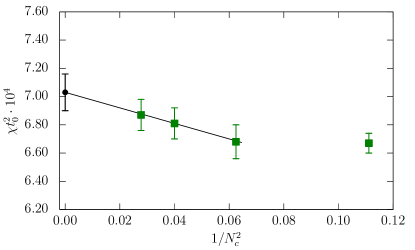
Figure 10: Scaling of the topological susceptibility with the number of colours in the pure Yang-Mills theory. The dashed line is a linear fit in $1/N_{c}^{2}$ including up to $N_{c}=4$. Source: Ref. Ce:2016awn for $N_{c}>3$ and Ref. Ce:2015qha at $N_{c}=3$.

The first computation of the topological susceptibility in the large $N_{c}$ limit was attempted two decades ago, in Ref. Lucini:2004yh . One of the main difficulties is the critical slowing down Schaefer:2010hu , that is, the very long autocorrelation time in topological observables as one approaches the continuum limit using periodic boundary conditions. This is already present in $N_{c}=3$, and it becomes more severe for $N_{c}>3$.

The use of open boundary conditions Luscher:2011kk significantly improves this situation, and has been an essential ingredient in the recent computation of $\chi_{YM}$ in the continuum limit Ce:2015qha ; Ce:2016awn . In Fig. 10, we show the continuum result of $\chi_{YM}$ as a function of the number of colours. The large-$N_{c}$ result reported by the authors is

$$\lim_{N_{c}\to\infty}t_{0}^{2}\chi_{YM}=7.03(13)\cdot 10^{-4},$$ (46)

which differs from the $N_{c}=3$ result by only about $O(5\%)$. As pointed out by the authors, the small size of $1/N_{c}^{2}$ effects explains why the $N_{c}=3$ result is already able to predict the bulk result of the $\eta^{\prime}$ mass. A lattice test of the Witten-Veneziano equation, computing directly the $\eta^{\prime}$ mass, has also been carried out in Ref. Cichy:2015jra for $N_{c}=3$.

The large-$N_{c}$ topological susceptibity has also been studied through the $\theta$-dependence in Refs. DelDebbio:2002xa ; Bonati:2016tvi ; Kitano:2020mfk , and in lower dimensional theories in Refs. Bonati:2019ylr ; Bonanno:2018xtd .

5 Hadronic quantities at large $N_{c}$

Here, we review recent results of hadronic quantities in the context of the large $N_{c}$ limit of QCD. We start with the meson and baryon spectrum. Then we discuss the chiral dependence of the meson masses, decay constants, scattering lengths and the topological susceptibility. We then turn to novel results on weak amplitudes related to the $\Delta I=1/2$ rule.

5.1 Meson spectrum

The simplest question one may ask regarding hadrons is how the spectrum depends on the number of colours. As already discussed, all mesons are expected to become stable particles at large $N_{c}$, and thus they may be treated as asymptotic states, rather than resonances.

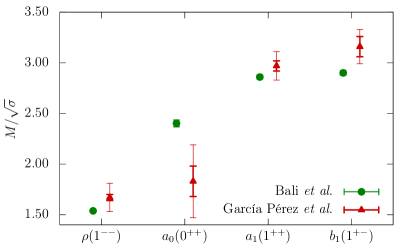
Figure 11: Large $N_{c}$ meson spectrum in different channels, with $J^{PC}$ as provided in the x-labels. We compare the results from standard large-$N_{c}$ approach from Ref. Bali:2013kia , to the ones obtained using the Twisted Eguchi-Kawai reduction Perez:2020vbn . In the case of Ref. Perez:2020vbn , the smaller errorbars are statistical, whereas the larger ones include the systematics of chiral and continuum extrapolation.

The most extensive study of the meson spectrum was performed in Ref. Bali:2013kia . It was done using the quenched approximation at a fixed lattice spacing. Although it is known that quenching alters some $1/N_{c}$ corrections, the strict large $N_{c}$ limit is the same for both the dynamical and quenched theory (with fundamental fermions). More recently, large $N_{c}$ results from reduced models Perez:2020fqn ; Perez:2020vbn were made public. We compare the results of the two approaches in Fig. 11. As can be seen, there is a reasonable overall agreement, with differences of at most $2\sigma$. It must be noted that while Ref. Bali:2013kia has better statistical accuracy, the results may be affected by significant discretization errors. In contrast, those of Ref. Perez:2020vbn are in the continuum limit.

Another interesting observation is the one of Ref. Nogradi:2019iek . The authors found that the ration $M_{\rho}/F_{\pi}$ in the chiral limit seemed independent on $N_{f}$ in $N_{c}=3$:

$$\frac{M_{\rho}}{F_{\pi}}\Bigg{\rvert}^{N_{f}=2-6}_{N_{c}=3}=7.95(15),$$ (47)

whereas at large $N_{c}$, the following result is found Bali:2013kia :

$$\sqrt{\frac{N_{c}}{3}}\frac{M_{\rho}}{F_{\pi}}\Bigg{\rvert}_{N_{c}\to\infty}=7.08(10).$$ (48)

The comparison of the previous equation indicates that both, $1/N^{2}_{c}$ and $N_{f}/N_{c}$ effects are rather small in this ratio. This is consistent with the result of Ref. Nogradi:2019auv , where the authors summarized the dependence on the gauge group and fermionic representation of the same quantity using all existing lattice data Appelquist:2018yqe ; Fodor:2016pls ; Bali:2013kia ; Ayyar:2017qdf ; Drach:2017btk ; Amato:2018nvj ; Bennett:2019cxd ; Bennett:2019jzz . They pointed out that it is almost constant up to a trivial factor that depends on the dimensionality of the fermion fields—$\sqrt{N_{c}}$ for $SU(N_{c})$. We should also mention that the result in eq. (48) is in the ballpark of predictions from a resonance chiral theory Ledwig:2014cla .

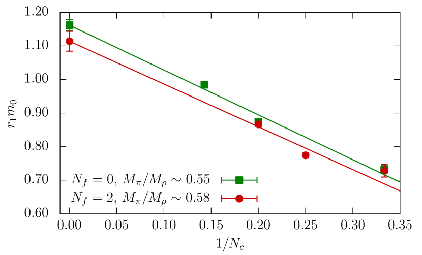
(a)

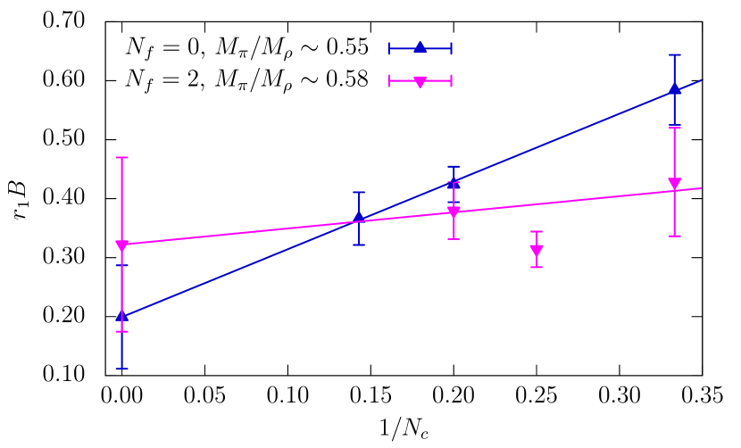
(b)

Figure 12: $1/N_{c}$-scaling of the constants $r_{1}m_{0}$ (top) and $r_{1}B$ (bottom) in eq. (49) for the quenched data in Ref. DeGrand:2013nna , and $N_{f}=2$ in Ref. DeGrand:2016pur . The simulations at different $N_{c}$ have been matched at approximately fixed $M_{\pi}/M_{\rho}$.

5.2 Baryons

A series of publications have studied the scaling of baryon masses with the number of colours: first, in the quenched approximation DeGrand:2012hd ; DeGrand:2013nna ; Cordon:2014sda , and more recently with dynamical quarks ($N_{f}=2$) DeGrand:2016pur . These have been carried out at a single lattice spacing. In a generic $SU(N_{c})$ theory, the spin of the baryon can take half-integer for odd $N_{c}$ (fermionic baryons, as in QCD), or integer values for even $N_{c}$ (bosonic baryons).

It has been long known Jenkins:1993zu that baryon masses depend on their angular momentum. This is the so-called hyperfine splitting, which for the case of two degenerate quarks takes the form:

$$M_{B}(N_{c},J)=N_{c}m_{0}(N_{c})+\frac{J(J+1)}{N_{c}}B+\cdots,$$ (49)

with $m_{0},B$ being $O(N_{c}^{0})$ constants. Note that they can have a subleading $N_{c}$ dependence, for instance, for $m_{0}$:

$$m_{0}=m_{0}^{(0)}+\frac{m_{0}^{(1)}}{N_{c}}+\ldots,$$ (50)

and similarly for $B$. Generalizations of the eq. (49) that incorporate the strange quark also exist in the literature Dai:1995zg ; Jenkins:1995td . The constants in eq. (49) can be isolated by taking appropriate combinations, for instance:

$$\begin{split}m_{0}&=\frac{1}{4N_{c}}\left[5M(N_{c},1/2)-M(N_{c},3/2)\right],\\ B&=\frac{3}{N_{c}}\left[M(N_{c},1/2)-M(N_{c},3/2)\right].\end{split}$$ (51)

The general conclusions of Refs. DeGrand:2012hd ; DeGrand:2013nna is that the qualitative expectations of large $N_{c}$ are satisfied by the data, including those of the $SU(3)$-flavour breaking due to the strange quark. In Ref. Cordon:2014sda , combined chiral and $N_{c}$ fits of the mass and hyperfine splitting were performed, using a consistent expansion in Baryon Chiral Perturbation Theory. That study was able to constrain some of the subleading low-energy constants (LECs).

As an example, we show in Fig. 12 the scaling of $m_{0}$ and $B$ with the number of colours for the quenched and dynamical baryons at approximately fixed Sommer scale $r_{1}$ Bernard:2000gd and $M_{\pi}/M_{\rho}$. As can be seen from the plots, quenched and $N_{f}=2$ results for $r_{1}m_{0}$ agree at fixed $N_{c}$, and in the large $N_{c}$ extrapolation. For $r_{1}B$, uncertainties are larger, and some quenching effects may be appreciated. We stress that relative discretization errors may be large, and so, this comparison must be taken as qualitative.

It is also worth mentioning that there have been lattice studies of baryons in the context of BSM physics. These have focused on studying a $SU(4)$ gauge theory with both two fundamental and two sextet fermions Appelquist:2014jch ; DeGrand:2015lna ; Ayyar:2018zuk . This model represents a slight simplification of the asymptotically-free composite-Higgs Ferretti model Ferretti:2013kya ; Ferretti:2014qta .

5.3 Chiral and $N_{c}$ dependence of light meson observables

In Ref. Hernandez:2019qed , a first-principles calculation of the $N_{c}$ scaling of the low-energy couplings (LECs) of the chiral Lagrangian has been presented. The LECs are extracted from the chiral dependence of meson masses and decay constants. The lattice setup of this work is $N_{f}=4$, with $O(a)$-improved Wilson fermions in the sea, and mixed action with twisted mass in the valence. This has the advantage of automatic $O(a)$ improvement, avoiding the need of non-perturbative renormalization factors.

First the authors consider each value of $N_{c}$ separately. They perform a chiral fit of the data points to extract the LO and NLO low-energy constants appearing in the NLO chiral predictions Bijnens1 ; Bijnens2 ; Bijnens3 of $F_{\pi}$ and $M_{\pi}$:

$$F_{\pi} ={F}\Bigg{[}1-{\frac{N_{f}}{2}\frac{M_{\pi}^{2}}{(4\pi F_{\pi})^{2}}\log\frac{M_{\pi}^{2}}{\mu^{2}}}+4\frac{M_{\pi}^{2}}{F_{\pi}^{2}}L_{F}\Bigg{]},$$ (52)

$$\frac{M^{2}_{\pi}}{\mu} =2B\Bigg{[}1+{\frac{1}{N_{f}}\frac{M_{\pi}^{2}}{(4\pi F_{\pi})^{2}}\log\frac{M_{\pi}^{2}}{\mu^{2}}}+8\frac{M_{\pi}^{2}}{F_{\pi}^{2}}L_{M}\Bigg{]}.$$ (53)

Here, $B$ and $F$ are the chiral condensate and decay constant in the chiral limit; $\mu$ is the quark mass, and $L_{M}$, $L_{F}$ are combinations the standard LEC:

$$L_{F}=L_{5}^{r}+N_{f}L_{4}^{r},\ \ \ L_{M}=2L_{8}^{r}-L_{5}^{r}+N_{f}(2L_{6}^{r}-L_{4}^{r}).$$ (54)

The scaling with the number of colours of these quantities is known: $F^{2},L_{5}$ and $L_{8}$ are $O(N_{c})$, while $B,L_{4}$ and $L_{6}$ are $O(N_{c}^{0})$. The results of these fits are shown in Figs. 13(a) and 13(b). One can see that the scaling is well described by leading and subleading $N_{c}$ corrections for $N_{c}=4-6$, while there seems to be significant $1/N_{c}^{2}$ corrections for $N_{c}=3$ in the case of $F$ and $L_{F}$. In the case of $B$ and $L_{M}$, there is no sign of $1/N_{c}^{2}$ effects.

As explained in sec. 2.2, the chiral regime at large $N_{c}$ requires the addition of the $\eta^{\prime}$, and a combined power counting of the usual momentum/mass expansion with that in $1/N_{c}$. Using the standard power-counting DiVecchia:1980yfw ; PhysRevD.21.3388 ; Witten:1980sp ; Kawarabayashi:1980dp ; HerreraSiklody:1996pm ; Kaiser:2000gs

$$\mathcal{O}(\delta)\sim\mathcal{O}(m_{q})\sim\mathcal{O}(p^{2})\sim\mathcal{O}(M_{\pi}^{2})\sim\mathcal{O}(1/N_{c}),$$ (55)

the $\mathcal{O}(\delta^{2})$ predictions are:

$$F_{\pi} =\sqrt{N_{c}}\left({F}_{0}+{{F}_{1}\over N_{c}}+{{F}_{2}\over N_{c}^{2}}\right)\Bigg{[}1-{\frac{N_{f}}{2}\frac{M_{\pi}^{2}}{(4\pi F_{\pi})^{2}}\log\frac{M_{\pi}^{2}}{\mu^{2}}}$$

$$+ 4\frac{M_{\pi}^{2}}{F_{\pi}^{2}}\Big{(}N_{c}{L}_{F}^{(0)}+{L}_{F}^{(1)}\Big{)}+N_{c}^{2}K_{F}^{(0)}\left({M_{\pi}^{2}\over F_{\pi}^{2}}\right)^{2}$$

$$+ \ {\mathcal{O}}(\delta^{3})\Bigg{]},$$

and

$$M^{2}_{\pi} =2m\left({B}_{0}+{{B}_{1}\over N_{c}}+{{B}_{2}\over N_{c}^{2}}\right)\Bigg{[}$$

$$1 +{\frac{1}{N_{f}}\frac{M_{\pi}^{2}}{(4\pi F_{\pi})^{2}}\log\frac{M_{\pi}^{2}}{\mu^{2}}}-{\frac{1}{N_{f}}\frac{M_{\eta^{\prime}}^{2}}{(4\pi F_{\pi})^{2}}\log\frac{M_{\eta^{\prime}}^{2}}{\mu^{2}}}$$

$$+ 8\frac{M_{\pi}^{2}}{F_{\pi}^{2}}\Big{(}N_{c}{L}_{M}^{(0)}+{L}_{M}^{(1)}\Big{)}+N_{c}^{2}K_{M}^{(0)}\left({M_{\pi}^{2}\over F_{\pi}^{2}}\right)^{2}+{\mathcal{O}}(\delta^{3})\Bigg{]}.$$

Here, $F_{i},B_{i},L_{M}^{(i)}$ and $L_{F}^{(i)}$ are the coefficients of the $1/N_{c}$ expansion of the corresponding LECs. $K_{F,M}$ are combinations of LECs that contribute at $\mathcal{O}(M_{\pi}^{4})$.. A global chiral fit of all $N_{c}$ data to these expressions is shown in Fig. 14. The ChPT predictions seem to describe data well.

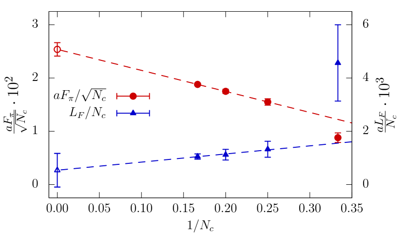
(a) LECs of the decay constant.

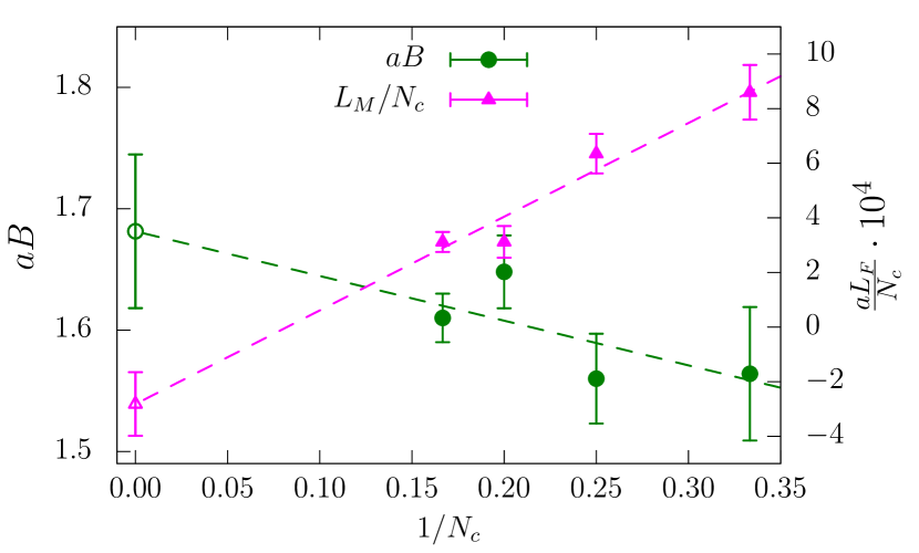
(b) LECs of the meson mass.

Figure 13: $1/N_{c}$ scaling of the LO and NLO low-energy constants extracted from fits to eqs.  (52) and (53) at a fixed value of $N_{c}$. Source: Ref. Hernandez:2019qed .

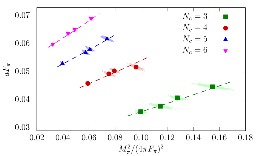
(a)

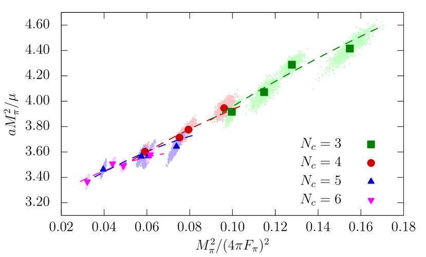
(b)

Figure 14: Simultaneous chiral and $N_{c}$ fits of the decay constant (left) and the pion mass (right). Bootstrap samples are shown as “clouds” around the central value. The fit equations are linearized versions of eqs. (5.3) and (5.3). More detail on the fitting strategy is give in the original article, Ref. Hernandez:2019qed .

An interesting observation of Ref. Hernandez:2019qed is that by studying the first coefficients in the $1/N_{c}$ expansion, one can infer the values of some quantities at different value of $N_{f}$, since the leading corrections come from fermion loops and are therefore of the form $N_{f}/N_{c}$ (the non-planar gluonic corrections start at $1/N_{c}^{2}$). The simplest example is the decay constant in the chiral limit, whose leading $N_{f},N_{c}$ dependence is:

$$\frac{F}{\sqrt{N_{c}}}=F_{0}+\widetilde{F}_{1}\frac{N_{f}}{N_{c}}+\cdots.$$ (58)

Since $\widetilde{F}_{1}$ is trivially related by a factor $N_{f}$ to one of the fit parameters in eq. (5.3), the authors are able to quote inferred results for $N_{f}=2$ and $3$:

$$\begin{split}&F^{N_{c}=3,N_{f}=2}=81(7)\text{ MeV},\\ &F^{N_{c}=3,N_{f}=3}=68(7)\text{ MeV},\end{split}$$ (59)

which are in good agreement with phenomenological and lattice determinations—see Ref. Aoki:2019cca . The same strategy is followed for the LECs, and the chiral condensate.

We should also mention that the chiral behaviour of $F_{\pi}$ in $N_{f}=2$ simulations (and the equivalent for vector meson) was also studied at in Ref. DeGrand:2016pur , albeit no chiral fits were performed.

Another quantity that may be explored are meson scattering amplitudes. Although they vanish in the exact large $N_{c}$ limit, it is interesting to study the subleading $N_{c}$ behaviour, and the interplay with the quark mass dependence. For instance, the isospin-2 leading order ChPT prediction is

$$M_{\pi}a_{0}^{I=2}=\frac{M_{\pi}^{2}}{16\pi F_{\pi}^{2}}\sim O\left(\frac{1}{N_{c}}\right),$$ (60)

that is consistent with the $N_{c}$-scaling discussed in sec. 2.2.

In finite volume, scattering amplitudes may be obtained with the Lüscher formalism Luscher:1986pf , and generalizations thereof (see Ref. Briceno:2017max for a review). In the so-called threshold (or $1/L$) expansion, valid for weakly interacting systems, it is possible to relate the finite-volume energy shift of the two-particle ground state to the scattering length by to the scattering length, see Ref. Luscher:1986pf .

Recently, preliminary results for the isospin-2 scattering length at $N_{c}=3-6$ have been presented Romero-Lopez:2019gqt . As $N_{c}$ grows, two different effects compete. The signal for the energy shift becomes weaker as the scattering length decreases, but the statistical error gets reduced as a result of the increase of gluonic degrees of freedom. In Ref.  Romero-Lopez:2019gqt $a_{0}^{I=2}$ at $N_{c}>3$ was obtained with good accuracy, and a remarkable agreement with leading order ChPT [see eq. (60)] was found.

Additional channels, such as the isospin-0 ($\sigma$) channel may represent an interesting problem to study in the large $N_{c}$ context. It has been argued that the $N_{c}$-scaling may shed light on the nature of the $\sigma$ resonance Pelaez:2010er ; Nebreda:2011cp ; Bernard:2010fp ; RuizdeElvira:2017aet . Another very interesting application would be the study of tetraquarks with different flavour content in the planar limit PhysRevLett.110.261601 ; PhysRevD.88.036016 .

Finally, we should mention the results for the $\rho$ and the isospin-2 channels in $SU(2)$Janowski:2019svg ; Arthur:2014zda . Note that in this case the symmetry breaking pattern for $N_{c}=2$ is different than the one in $N_{c}>3$, and so effective field theory expectations differ.

5.4 Topological susceptibility with dynamical quarks

The topological susceptibility is an observable that has a very different behaviour in the pure Yang-Mills theory and in QCD with light quarks. In the former, discussed in sec. 4.3, $\chi_{YM}$ depends only weakly in the number of colours; whereas in the latter, it vanishes in the chiral limit for all values of $N_{c}$. It has been predicted DiVecchia:1980yfw ; Leutwyler:1992yt ; Crewther:1977ce that the topological susceptibility mass-dependence is as follows:

$$\frac{1}{\chi(M_{\pi})}=\frac{2N_{f}}{F^{2}_{\pi}M_{\pi}^{2}}+\frac{1}{\chi_{YM}}.$$ (61)

In the previous equation, the pure gauge (quenched) limit is achieved by letting $M_{\pi}\to\infty$, whereas at small pion mass, one simply has $\chi(M_{\pi})\propto M_{\pi}^{2}$.

Figure 15: Topological susceptibility as a function of the pion mass in $N_{f}=2$ QCD. The solid line is the functional form in eq. (61), using the continuum results of Refs. Ce:2015qha ; Bruno:2014ova . The dashed lines are the expectations in the two regimes (quenched and light pions). The various coloured points are the results of Ref. DeGrand:2020utq with $N_{c}=3-5$.

The topological susceptibility with dynamical fermions has been studied for $N_{c}=3$ Durr:2001ty ; Chiu:2011dz ; Bruno:2014ova ; Aoki:2007pw . The most recent result Bruno:2014ova , includes a continuum limit extrapolation. In the present year, a “pilot study” with varying $N_{c}=3-5$ DeGrand:2020utq was also published.

Combining the results in the Yang-Mills theory Ce:2015qha , with the $N_{f}=2$ ones Bruno:2014ova one can produce an interpolating curve between the two regimes based on eq. (61). This can be compared to the results of Ref. DeGrand:2020utq with $N_{c}=3-5$. As can be seen, qualitative (but not quantitative) agreement is observed. One possibility to explain the disagreement are discrezation effects, which were found in Ref. Bruno:2014ova to be relevant with the Wilson fermionic action. Finite volume effects may also be significant in Ref. DeGrand:2020utq .

5.5 The $\Delta I=1/2$ rule

In the last few years, impressive progress has been achieved in the lattice determination of the $K\rightarrow\pi\pi$ amplitudes, and the related CP violation observable $\epsilon^{\prime}/\epsilon$ Boyle:2012ys ; Bai:2015nea ; Blum:2015ywa ; Ishizuka:2018qbn ; Abbott:2020hxn . The $\Delta I=1/2$ enhancement seems to be reproduced by the latest simulations at the physical point in $2+1$ simulations with a heavy charm Abbott:2020hxn .

In an earlier work Boyle:2012ys , an analysis of the various contributions to $K\to\pi\pi$ suggested that the main source of the enhancement comes from the current-current operators, eqs. (26). It emerges from a strong cancellation of the isospin-2 amplitude, as a result of a negative relative sign between the colour-connected and colour-disconnected contractions, which scale differently in large $N_{c}$. The scaling in $N_{c}$ of these amplitudes allows therefore to disentangle the two contributions rigorously, and has been studied in Refs. Donini:2016lwz ; Donini:2020qfu .

In these studies an old strategy Giusti:2004an ; Giusti:2006mh was revisited in the context of large $N_{c}$, where a light active charm, mass-degenerate with the up quark, was included, simplifying enormously the calculation. In this scenario, only the two current-current operators, $Q^{\pm}$, fully describe the $\Delta S=1$ transitions. A matching to $N_{f}=4$ chiral perturbation theory, allows to extract the low-energy couplings, $g^{\pm}$, representing the strength of these interactions in the chiral Lagrangian, eq. (29). The couplings can be extracted from the measurement of the simpler $K\to\pi$ amplitudes, $A^{\pm}$ in the chiral limit. The determination of $g^{\pm}$ gives then an indirect estimate of the $K\to\pi\pi$ isospin amplitudes.

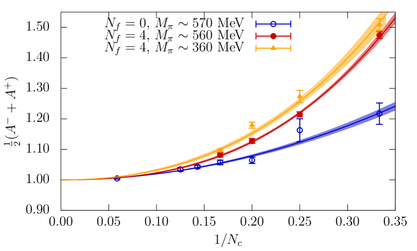
(a)

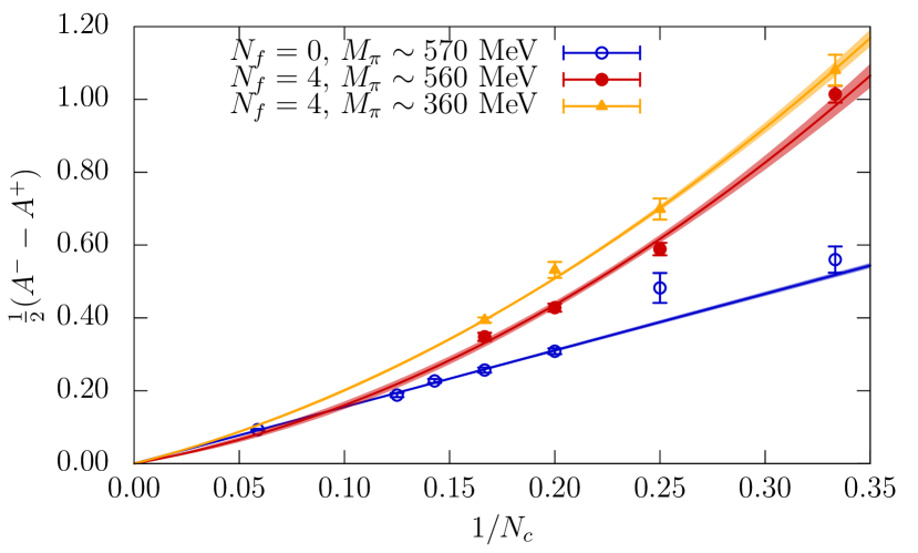
(b)

Figure 16: Half-sum and half-difference of the amplitudes $A^{\pm}$ as a function of $N_{c}$ for three different cases: (i) quenched results in blue, (ii) dynamical results at a pion similar to the quenched case (red), and (iii) dynamical results at a lighter pion mass (orange). Error bars include only statistical errors. Source: Refs. Donini:2016lwz ; Donini:2020qfu .

(a)

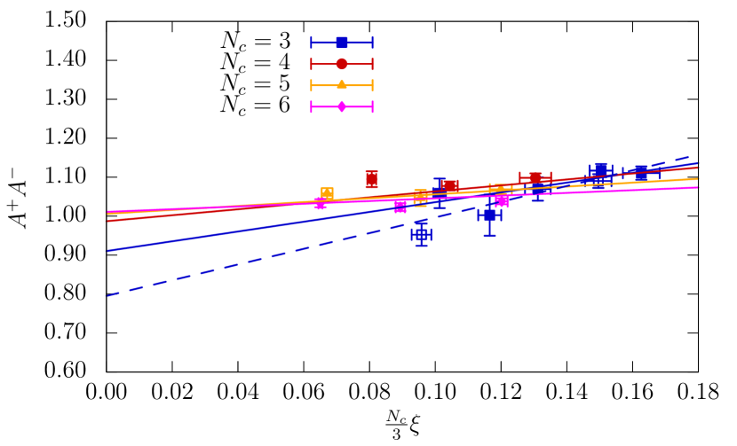
(b)

Figure 17: Chiral extrapolation of $A^{+}$ and the product $A^{+}A^{-}$. Empty squares for $N_{c}=3$ indicate a finer lattice spacing. Solid lines indicate a simultaneous chiral and $N_{c}$ fit. Dashed lines represent the chiral extrapolation of the data points with $N_{c}=3$. Source: Ref. Donini:2020qfu ,

The expected large $N_{c}$ scaling of the amplitudes $A^{\pm}$ has been presented in eq. (34). By means of appropriate linear combinations, one can isolate the (anti-)correlated coefficients:

$$\frac{A^{-}+A^{+}}{2} =1+\tilde{c}\frac{1}{N_{c}^{2}}+\tilde{d}\frac{N_{f}}{N_{c}^{3}},$$ (62)

$$\frac{A^{-}-A^{+}}{2} =\tilde{a}\frac{1}{N_{c}}+\tilde{b}\frac{N_{f}}{N_{c}^{2}}.$$ (63)

The $N_{c}$ scaling of these combinations was analysed in Ref. Donini:2020qfu in three different scenarios: (i) quenched results ($N_{f}=0$) at a heavy pion mass $\sim 570$ MeV, (ii) dynamical results ($N_{f}=4$) at a heavy pion mass $\sim 560$ MeV, and (iii) dynamical results ($N_{f}=4$) at a lighter pion mass $\sim 360$ MeV. This can be seen in Fig. 16 and Table 1. The main conclusion from this study is that all coefficients turned out to be of the natural size. Importantly, the sign of the $\tilde{a}$ and $\tilde{b}$ coefficients is the same and negative. This implies that both terms contribute to reduce the $A^{+}$ amplitude and enhance, in a correlated way, the amplitude $A^{-}$. Moreover, it can be seen that the mass dependence for the $N_{f}=4$ results seems to affect mostly the coefficient $\tilde{a}$, and goes also in the direction of enhancing the ratio $A^{-}/A^{+}$ towards the chiral limit.

Half-difference
Case	$M_{\pi}$	$\tilde{a}$	$\tilde{b}$	$\chi^{2}/\text{d.o.f.}$
$N_{f}=0$	$570$ MeV	-1.55(2)	—	8.8/6
$N_{f}=4$	$560$ MeV	-1.03(13)	-1.44(13)	6.6/2
$N_{f}=4$	$360$ MeV	-1.49(15)	-1.32(18)	0.3/2

Half-sum
Case	$M_{\pi}$	$\tilde{c}$	$\tilde{d}$	$\chi^{2}/\text{d.o.f.}$
$N_{f}=0$	$570$ MeV	2.1(1)	—	3.5/6
$N_{f}=4$	$560$ MeV	1.2(3)	2.2(3)	1.3/2
$N_{f}=4$	$360$ MeV	2.4(4)	1.6(4)	3.2/2

Table 1: Summary of results for the $1/N_{c}$ fits to the half-sum and half-difference of the amplitudes $A^{\pm}$. Errors are only statistical.

The determination of the couplings $g^{\pm}$ requires an extrapolation to the chiral limit. The ChPT prediction for these amplitudes is Hernandez:2006kz ; Kambor:1989tz :

$$A^{\pm}=g^{\pm}\left[1+3\left(\frac{M_{\pi}}{4\pi F_{\pi}}\right)^{2}\log\frac{M_{\pi}^{2}}{\Lambda_{\pm}^{2}}\right].$$ (64)

The chiral fits are shown in Fig. 17 for the $A^{+}$ amplitude (Fig. 17(a)) and the product of the two $A^{+}A^{-}$ (Fig. 17(b)). The result for $N_{c}=3$ is:

$$\frac{g^{-}}{g^{+}}=22(5),$$ (65)

where the error is only statistical. Finally, an indirect estimate of the $K\to\pi\pi$ isospin amplitudes can be derived using the LO ChPT prediction in eq. (31), and also the NLO one derived in Ref. Donini:2020qfu . The final estimate of Ref. Donini:2020qfu for this ratio in the theory with a light charm is

$$\frac{A_{0}}{A_{2}}\Bigg{\rvert}_{N_{f}=4,N_{c}=3}=24(5)_{\text{stat}}(7)_{\text{sys}}.$$ (66)

The main conclusion from this work is that the large enhancement observed in the $\Delta I=1/2$ rule seems consistent with coefficients in the $1/N_{c}$ expansion that are of the natural size, but with an important effect coming from the quark loops. In addition, the result in eq. (66) suggests that the enhancement may indeed be largely dominated by intrinsic QCD effects, and not from the intermediate scale set by the charm quark mass.

6 Concluding remarks

We have reviewed recent lattice studies of the large $N_{c}$ limit of QCD. Our main focus has been the study of large $N_{c}$ scaling of various physical quantities at zero temperature, using the conventional approach of comparing standard lattice simulations at physical volumes and increasing values of $N_{c}$. Some of the results obtained with non-standard approaches, such as the Eguchi-Kawai reduction (and variations thereof), are also included in the comparison of results.

We have presented results in pure Yang-Mills, more specifically, a non-perturbative study of factorization, the glueball spectrum and the topological susceptibility. In the case of theories with fermions, results on the meson and baryon spectrum, the chiral behaviour of meson masses and decay constants, the topological susceptibility and some preliminary results on $\pi\pi$ scattering have been reviewed. We discussed in some detail a compelling new result on the $1/N_{c}$ scaling of weak amplitudes related to the $\Delta I=1/2$ rule in kaon decays.

In most of these cases, the expected scaling in $N_{c}$ is confirmed. Coefficients of the natural size are found, that is ${\mathcal{O}}(N_{c}^{-1})$ relative corrections. In particular, this is found to be the case for the ratio of isospin amplitudes in kaon decays. In some cases, however, the coefficients of the subleading corrections might be significantly enhanced when leading and subleading corrections do measure different physics scales. This is for example the case when studying violations to factorization.

In this respect one interesting direction for future work is the study of meson interactions with growing $N_{c}$. This involves not only pion scattering, but also glueball interactions and potential exotic resonances, such as tetraquarks, that may prevail at large $N_{c}$.

Finally we should mention other works that we have not reviewed, for instance, Ref. Athenodorou:2017cmw . A number of results at varying $N_{c}$ at finite-temperature exist Lucini:2003zr ; DelDebbio:2004vxo ; Lucini:2005vg ; Lucini:2012wq ; DeGrand:2018tzn ; Bonati:2013tt ; Datta:2010sq ; Bringoltz:2005rr ; Bonati:2019unv ; Bonati:2019kmf ; Bursa:2005yv ; Panero:2009tv ; Mykkanen:2012ri . Recent lattice results with different gauge groups and fermion content can be found in Holligan:2019lma ; Bennett:2020hqd ; Ayyar:2018glg ; Brower:2020mab .

Acknowledgements

We warmly thank T. DeGrand, M. García-Pérez, M. García Vera, C. Pena, A. Ramos and R. Sommer for useful discussions.

We acknowledge support from the Generalitat Valenciana grant PROMETEO/2019/083, the European project H2020-MSCA-ITN-2019//860881-HIDDeN, and the Spanish project FPA2017-85985-P.

The work of FRL has also received funding from the EU Horizon 2020 research and innovation program under the Marie Skłodowska-Curie grant agreement No. 713673 and La Caixa Foundation (ID 100010434). FRL also acknowledges financial support from Generalitat Valenciana through the plan GenT program (CIDEGENT/2019/040).

References

- (1) G. ’t Hooft, Nucl. Phys. B72, 461 (1974), [,337(1973)]
- (2) T. Eguchi, H. Kawai, Phys. Rev. Lett. 48, 1063 (1982)
- (3) E. Witten, Nucl. Phys. B 160, 57 (1979)
- (4) S.R. Coleman, 1/N, in 17th International School of Subnuclear Physics: Pointlike Structures Inside and Outside Hadrons (1980), p. 0011
- (5) M.J. Teper, Phys. Rev. D 59, 014512 (1999), hep-lat/9804008
- (6) M. Garcia Perez, PoS LATTICE2019, 276 (2020), 2001.10859
- (7) M. Panero, PoS LATTICE2012, 010 (2012), 1210.5510
- (8) B. Lucini, M. Panero, Phys. Rept. 526, 93 (2013), 1210.4997
- (9) B. Lucini, Nucl. Part. Phys. Proc. 273-275, 1657 (2016), 1412.6086
- (10) T. DeGrand, E.T. Neil, Phys. Rev. D 101, 034504 (2020), 1910.08561
- (11) V. Drach, PoS LATTICE2019, 242 (2020), 2005.01002
- (12) G.D. Kribs, E.T. Neil, Int. J. Mod. Phys. A 31, 1643004 (2016), 1604.04627
- (13) S.R. Coleman, E. Witten, Phys. Rev. Lett. 45, 100 (1980)
- (14) J. Gasser, H. Leutwyler, Nucl. Phys. B 250, 465 (1985)
- (15) S. Peris, E. de Rafael, Phys. Lett. B 348, 539 (1995), hep-ph/9412343
- (16) G. Ecker, J. Gasser, A. Pich, E. de Rafael, Nucl. Phys. B 321, 311 (1989)
- (17) A. Pich, Colorless mesons in a polychromatic world, in The Phenomenology of Large N(c) QCD (2002), pp. 239–258, hep-ph/0205030
- (18) P. Di Vecchia, G. Veneziano, Nucl. Phys. B 171, 253 (1980)
- (19) C. Rosenzweig, J. Schechter, C.G. Trahern, Phys. Rev. D 21, 3388 (1980)
- (20) E. Witten, Annals Phys. 128, 363 (1980)
- (21) K. Kawarabayashi, N. Ohta, Nucl. Phys. B 175, 477 (1980)
- (22) H. Leutwyler, Phys. Lett. B 374, 163 (1996), hep-ph/9601234
- (23) P. Herrera-Siklody, J. Latorre, P. Pascual, J. Taron, Nucl. Phys. B 497, 345 (1997), hep-ph/9610549
- (24) R. Kaiser, H. Leutwyler, Eur. Phys. J. C 17, 623 (2000), hep-ph/0007101
- (25) E. Witten, Nucl. Phys. B 156, 269 (1979)
- (26) G. Veneziano, Nucl. Phys. B 159, 213 (1979)
- (27) L. Giusti, G. Rossi, M. Testa, G. Veneziano, Nucl. Phys. B 628, 234 (2002), hep-lat/0108009
- (28) E. Seiler, Phys. Lett. B 525, 355 (2002), hep-th/0111125
- (29) L. Giusti, G. Rossi, M. Testa, Phys. Lett. B 587, 157 (2004), hep-lat/0402027
- (30) M. Luscher, Phys. Lett. B 593, 296 (2004), hep-th/0404034
- (31) L. Del Debbio, L. Giusti, C. Pica, Phys. Rev. Lett. 94, 032003 (2005), hep-th/0407052
- (32) R.F. Dashen, E.E. Jenkins, A.V. Manohar, Phys. Rev. D 49, 4713 (1994), [Erratum: Phys.Rev.D 51, 2489 (1995)], hep-ph/9310379
- (33) E.E. Jenkins, Phys. Lett. B 315, 441 (1993), hep-ph/9307244
- (34) C. Carone, H. Georgi, S. Osofsky, Phys. Lett. B 322, 227 (1994), hep-ph/9310365
- (35) R.F. Dashen, E.E. Jenkins, A.V. Manohar, Phys. Rev. D 51, 3697 (1995), hep-ph/9411234
- (36) J. Dai, R.F. Dashen, E.E. Jenkins, A.V. Manohar, Phys. Rev. D 53, 273 (1996), hep-ph/9506273
- (37) E. Corrigan, P. Ramond, Phys. Lett. B 87, 73 (1979)
- (38) A.V. Manohar, Large N QCD, in Les Houches Summer School in Theoretical Physics, Session 68: Probing the Standard Model of Particle Interactions (1998), pp. 1091–1169, hep-ph/9802419
- (39) S. Weinberg, Phys. Rev. Lett. 110, 261601 (2013)
- (40) M. Knecht, S. Peris, Phys. Rev. D 88, 036016 (2013)
- (41) R.C. Brower, G. Maturana, M. Belen Gavela, R. Gupta, Phys. Rev. Lett. 53, 1318 (1984)
- (42) P. Boyle et al. (RBC, UKQCD), Phys. Rev. Lett. 110, 152001 (2013), 1212.1474
- (43) Z. Bai et al. (RBC, UKQCD), Phys. Rev. Lett. 115, 212001 (2015), 1505.07863
- (44) T. Blum et al., Phys. Rev. D 91, 074502 (2015), 1502.00263
- (45) N. Ishizuka, K.I. Ishikawa, A. Ukawa, T. Yoshié, Phys. Rev. D 98, 114512 (2018), 1809.03893
- (46) R. Abbott et al. (RBC, UKQCD), Phys. Rev. D 102, 054509 (2020), 2004.09440
- (47) M. Fukugita, T. Inami, N. Sakai, S. Yazaki, Phys. Lett. B 72, 237 (1977)
- (48) R. Chivukula, J. Flynn, H. Georgi, Phys. Lett. B 171, 453 (1986)
- (49) M.K. Gaillard, B.W. Lee, Phys. Rev. Lett. 33, 108 (1974)
- (50) G. Altarelli, L. Maiani, Phys. Lett. 52B, 351 (1974)
- (51) G. Buchalla, A.J. Buras, M.E. Lautenbacher, Rev. Mod. Phys. 68, 1125 (1996), hep-ph/9512380
- (52) A. Vainshtein, V.I. Zakharov, M.A. Shifman, JETP Lett. 23, 602 (1976)
- (53) W.A. Bardeen, A.J. Buras, J.M. Gerard, Nucl. Phys. B293, 787 (1987)
- (54) L. Giusti, P. Hernández, M. Laine, P. Weisz, H. Wittig, JHEP 11, 016 (2004), hep-lat/0407007
- (55) L. Giusti, P. Hernández, M. Laine, C. Pena, J. Wennekers, H. Wittig, Phys. Rev. Lett. 98, 082003 (2007), hep-ph/0607220
- (56) C.W. Bernard, T. Draper, A. Soni, H. Politzer, M.B. Wise, Phys. Rev. D 32, 2343 (1985)
- (57) W.A. Bardeen, A.J. Buras, J.M. Gérard, Phys. Lett. B180, 133 (1986)
- (58) A.J. Buras, J.M. Gérard, W.A. Bardeen, Eur. Phys. J. C 74, 2871 (2014), 1401.1385
- (59) V. Antonelli, S. Bertolini, J. Eeg, M. Fabbrichesi, E. Lashin, Nucl. Phys. B 469, 143 (1996), hep-ph/9511255
- (60) V. Cirigliano, G. Ecker, H. Neufeld, A. Pich, J. Portoles, Rev. Mod. Phys. 84, 399 (2012), 1107.6001
- (61) L. Del Debbio, A. Patella, C. Pica, Phys. Rev. D 81, 094503 (2010), 0805.2058
- (62) L. Del Debbio, B. Lucini, A. Patella, C. Pica, A. Rago, Phys. Rev. D 80, 074507 (2009), 0907.3896
- (63) B. Lucini, M. Teper, JHEP 06, 050 (2001), hep-lat/0103027
- (64) B. Lucini, M. Teper, U. Wenger, JHEP 01, 061 (2004), hep-lat/0307017
- (65) B. Lucini, G. Moraitis, Phys. Lett. B 668, 226 (2008), 0805.2913
- (66) P. Hernández, C. Pena, F. Romero-López, Eur. Phys. J. C79, 865 (2019), 1907.11511
- (67) A. Donini, P. Hernández, C. Pena, F. Romero-López, Eur. Phys. J. C80, 638 (2020), 2003.10293
- (68) G. Bhanot, U.M. Heller, H. Neuberger, Physics Letters B 113, 47 (1982)
- (69) R. Narayanan, H. Neuberger, Phys. Rev. Lett. 91, 081601 (2003), hep-lat/0303023
- (70) P. Kovtun, M. Unsal, L.G. Yaffe, JHEP 06, 019 (2007), hep-th/0702021
- (71) M. Unsal, L.G. Yaffe, Phys. Rev. D 78, 065035 (2008), 0803.0344
- (72) A. Gonzalez-Arroyo, M. Okawa, Physics Letters B 120, 174 (1983)
- (73) A. Gonzalez-Arroyo, M. Okawa, Phys. Rev. D 27, 2397 (1983)
- (74) A. Gonzalez-Arroyo, M. Okawa, JHEP 12, 106 (2014), 1410.6405
- (75) A. Gonzalez-Arroyo, M. Okawa, Physics Letters B 133, 415 (1983)
- (76) K. Fabricius, O. Haan, Physics Letters B 139, 293 (1984)
- (77) A. Gonzalez-Arroyo, M. Okawa, Phys. Lett. B 718, 1524 (2013), 1206.0049
- (78) A. González-Arroyo, M. Okawa, Phys. Lett. B 755, 132 (2016), 1510.05428
- (79) A. Hietanen, R. Narayanan, R. Patel, C. Prays, Phys. Lett. B 674, 80 (2009), 0901.3752
- (80) G.S. Bali, F. Bursa, L. Castagnini, S. Collins, L. Del Debbio, B. Lucini, M. Panero, JHEP 06, 071 (2013), 1304.4437
- (81) L. Del Debbio, H. Panagopoulos, P. Rossi, E. Vicari, JHEP 01, 009 (2002), hep-th/0111090
- (82) B. Lucini, M. Teper, U. Wenger, JHEP 02, 033 (2005), hep-lat/0502003
- (83) C. Allton, M. Teper, A. Trivini, JHEP 07, 021 (2008), 0803.1092
- (84) B. Lucini, A. Rago, E. Rinaldi, Phys. Lett. B 712, 279 (2012), 1202.6684
- (85) R. Lohmayer, H. Neuberger, JHEP 08, 102 (2012), 1206.4015
- (86) M. Lüscher, JHEP 08, 071 (2010), [Erratum: JHEP 03, 092 (2014)], 1006.4518
- (87) R. Sommer, PoS LATTICE2013, 015 (2014), 1401.3270
- (88) R.V. Harlander, T. Neumann, JHEP 06, 161 (2016), 1606.03756
- (89) M. Bruno, R. Sommer (ALPHA), PoS LATTICE2013, 321 (2014), 1311.5585
- (90) M. Bruno, T. Korzec, S. Schaefer, Phys. Rev. D 95, 074504 (2017), 1608.08900
- (91) M. Cè, M. García Vera, L. Giusti, S. Schaefer, Phys. Lett. B 762, 232 (2016), 1607.05939
- (92) T. DeGrand, Phys. Rev. D 95, 114512 (2017), 1701.00793
- (93) A. Bazavov et al. (MILC), Rev. Mod. Phys. 82, 1349 (2010), 0903.3598
- (94) R. Sommer, Nucl. Phys. B 411, 839 (1994), hep-lat/9310022
- (95) C.W. Bernard, T. Burch, K. Orginos, D. Toussaint, T.A. DeGrand, C.E. DeTar, S.A. Gottlieb, U.M. Heller, J.E. Hetrick, B. Sugar, Phys. Rev. D 62, 034503 (2000), hep-lat/0002028
- (96) O. Bar, M. Golterman, Phys. Rev. D 89, 034505 (2014), [Erratum: Phys.Rev.D 89, 099905 (2014)], 1312.4999
- (97) M. García Vera, R. Sommer, Eur. Phys. J. C 79, 35 (2019), 1805.11070
- (98) M.F. García Vera, Ph.D. thesis, Humboldt U., Berlin (2017)
- (99) M. García Vera, R. Sommer, EPJ Web Conf. 175, 11018 (2018), 1710.06057
- (100) B. Lucini, A. Rago, E. Rinaldi, JHEP 08, 119 (2010), 1007.3879
- (101) A. Athenodorou, M. Teper (2020), 2007.06422
- (102) A. Soni, Y. Zhang, Phys. Rev. D 93, 115025 (2016), 1602.00714
- (103) M.J. Teper (1998), hep-th/9812187
- (104) B. Lucini, M. Teper, U. Wenger, JHEP 06, 012 (2004), hep-lat/0404008
- (105) H.B. Meyer, M.J. Teper, Phys. Lett. B 605, 344 (2005), hep-ph/0409183
- (106) H.B. Meyer, Other thesis (2004), hep-lat/0508002
- (107) A. Amato, G. Bali, B. Lucini, PoS LATTICE2015, 292 (2016), 1512.00806
- (108) L. Del Debbio, G.M. Manca, H. Panagopoulos, A. Skouroupathis, E. Vicari, JHEP 06, 005 (2006), hep-th/0603041
- (109) H.B. Meyer, JHEP 03, 064 (2005), hep-lat/0412021
- (110) N. Yamanaka, H. Iida, A. Nakamura, M. Wakayama, PoS LATTICE2019, 013 (2019), 1911.03048
- (111) N. Yamanaka, H. Iida, A. Nakamura, M. Wakayama, Phys. Rev. D 102, 054507 (2020), 1910.07756
- (112) N. Yamanaka, H. Iida, A. Nakamura, M. Wakayama (2019), 1910.01440
- (113) C. Lovelace, Nucl. Phys. B 201, 333 (1982)
- (114) E. Bennett, J. Holligan, D.K. Hong, J.W. Lee, C.J.D. Lin, B. Lucini, M. Piai, D. Vadacchino, Phys. Rev. D 102, 011501 (2020), 2004.11063
- (115) Bennett, J. Holligan, D.K. Hong, J.W. Lee, C.J.D. Lin, B. Lucini, M. Piai, D. Vadacchino (2020), 2010.15781
- (116) M. Cè, C. Consonni, G.P. Engel, L. Giusti, Phys. Rev. D 92, 074502 (2015), 1506.06052
- (117) B. Lucini, M. Teper, U. Wenger, Nucl. Phys. B 715, 461 (2005), hep-lat/0401028
- (118) S. Schaefer, R. Sommer, F. Virotta (ALPHA), Nucl. Phys. B 845, 93 (2011), 1009.5228
- (119) C. Bonanno, C. Bonati, M. D’Elia (2020), 2012.14000
- (120) M. Luscher, S. Schaefer, JHEP 07, 036 (2011), 1105.4749
- (121) K. Cichy, E. Garcia-Ramos, K. Jansen, K. Ottnad, C. Urbach (ETM), JHEP 09, 020 (2015), 1504.07954
- (122) L. Del Debbio, H. Panagopoulos, E. Vicari, JHEP 08, 044 (2002), hep-th/0204125
- (123) C. Bonati, M. D’Elia, P. Rossi, E. Vicari, Phys. Rev. D 94, 085017 (2016), 1607.06360
- (124) R. Kitano, N. Yamada, M. Yamazaki (2020), 2010.08810
- (125) C. Bonati, P. Rossi, Phys. Rev. D 99, 054503 (2019), 1901.09830
- (126) C. Bonanno, C. Bonati, M. D’Elia, JHEP 01, 003 (2019), 1807.11357
- (127) M.G. Pérez, A. González-Arroyo, M. Okawa (2020), 2011.13061
- (128) M.G. Pérez, A. González-Arroyo, M. Okawa, PoS LATTICE2019, 113 (2019), 2001.00172
- (129) G.S. Bali, L. Castagnini, B. Lucini, M. Panero, PoS LATTICE2013, 100 (2014), 1311.7559
- (130) D. Nogradi, L. Szikszai, JHEP 05, 197 (2019), 1905.01909
- (131) D. Nogradi, L. Szikszai, PoS LATTICE2019, 237 (2019), 1912.04114
- (132) T. Appelquist et al. (Lattice Strong Dynamics), Phys. Rev. D 99, 014509 (2019), 1807.08411
- (133) Z. Fodor, K. Holland, J. Kuti, S. Mondal, D. Nogradi, C.H. Wong, PoS LATTICE2015, 219 (2016), 1605.08750
- (134) V. Ayyar, T. DeGrand, M. Golterman, D.C. Hackett, W.I. Jay, E.T. Neil, Y. Shamir, B. Svetitsky, Phys. Rev. D 97, 074505 (2018), 1710.00806
- (135) V. Drach, T. Janowski, C. Pica, EPJ Web Conf. 175, 08020 (2018), 1710.07218
- (136) A. Amato, V. Leino, K. Rummukainen, K. Tuominen, S. Tähtinen (2018), 1806.07154
- (137) E. Bennett, D.K. Hong, J.W. Lee, C.J.D. Lin, B. Lucini, M. Mesiti, M. Piai, J. Rantaharju, D. Vadacchino, Phys. Rev. D 101, 074516 (2020), 1912.06505
- (138) E. Bennett, D.K. Hong, J.W. Lee, C.J.D. Lin, B. Lucini, M. Piai, D. Vadacchino, JHEP 12, 053 (2019), 1909.12662
- (139) T. Ledwig, J. Nieves, A. Pich, E. Ruiz Arriola, J. Ruiz de Elvira, Phys. Rev. D 90, 114020 (2014), 1407.3750
- (140) T. DeGrand, Phys. Rev. D 89, 014506 (2014), 1308.4114
- (141) T. DeGrand, Y. Liu, Phys. Rev. D 94, 034506 (2016), [Erratum: Phys.Rev.D 95, 019902 (2017)], 1606.01277
- (142) T. DeGrand, Phys. Rev. D 86, 034508 (2012), 1205.0235
- (143) A.C. Cordón, T. DeGrand, J. Goity, Phys. Rev. D 90, 014505 (2014), 1404.2301
- (144) E.E. Jenkins, R.F. Lebed, Phys. Rev. D 52, 282 (1995), hep-ph/9502227
- (145) T. Appelquist et al. (Lattice Strong Dynamics (LSD)), Phys. Rev. D 89, 094508 (2014), 1402.6656
- (146) T. DeGrand, Y. Liu, E.T. Neil, Y. Shamir, B. Svetitsky, Phys. Rev. D 91, 114502 (2015), 1501.05665
- (147) V. Ayyar, T. Degrand, D.C. Hackett, W.I. Jay, E.T. Neil, Y. Shamir, B. Svetitsky, Phys. Rev. D 97, 114505 (2018), 1801.05809
- (148) G. Ferretti, D. Karateev, JHEP 03, 077 (2014), 1312.5330
- (149) G. Ferretti, JHEP 06, 142 (2014), 1404.7137
- (150) J. Bijnens, J. Lu, JHEP 11, 116 (2009), 0910.5424
- (151) J. Bijnens, J. Lu, JHEP 03, 028 (2011), 1102.0172
- (152) J. Bijnens, K. Kampf, S. Lanz, Nucl. Phys. B873, 137 (2013), 1303.3125
- (153) X.K. Guo, Z.H. Guo, J.A. Oller, J.J. Sanz-Cillero, JHEP 06, 175 (2015), 1503.02248
- (154) S. Aoki et al. (Flavour Lattice Averaging Group), Eur. Phys. J. C 80, 113 (2020), 1902.08191
- (155) M. Luscher, Commun. Math. Phys. 105, 153 (1986)
- (156) R.A. Briceno, J.J. Dudek, R.D. Young, Rev. Mod. Phys. 90, 025001 (2018), 1706.06223
- (157) F. Romero-López, A. Donini, P. Hernández, C. Pena, PoS LATTICE2019, 005 (2019), 1910.10418
- (158) J. Pelaez, J. Nebreda, G. Rios, Prog. Theor. Phys. Suppl. 186, 113 (2010), 1007.3461
- (159) J. Nebreda, J. Pelaez, G. Rios, Phys. Rev. D 84, 074003 (2011), 1107.4200
- (160) V. Bernard, M. Lage, U.G. Meissner, A. Rusetsky, JHEP 01, 019 (2011), 1010.6018
- (161) J. Ruiz de Elvira, U.G. Meißner, A. Rusetsky, G. Schierholz, Eur. Phys. J. C 77, 659 (2017), 1706.09015
- (162) T. Janowski, V. Drach, S. Prelovsek, PoS LATTICE2019, 123 (2019), 1910.13847
- (163) R. Arthur, V. Drach, M. Hansen, A. Hietanen, C. Pica, F. Sannino, PoS LATTICE2014, 271 (2014), 1412.4771
- (164) H. Leutwyler, A.V. Smilga, Phys. Rev. D 46, 5607 (1992)
- (165) R. Crewther, Phys. Lett. B 70, 349 (1977)
- (166) M. Bruno, S. Schaefer, R. Sommer (ALPHA), JHEP 08, 150 (2014), 1406.5363
- (167) T. DeGrand, Phys. Rev. D 101, 114509 (2020), 2004.09649
- (168) S. Durr, Nucl. Phys. B 611, 281 (2001), hep-lat/0103011
- (169) T.W. Chiu, T.H. Hsieh, Y.Y. Mao (TWQCD), Phys. Lett. B 702, 131 (2011), 1105.4414
- (170) S. Aoki et al. (JLQCD, TWQCD), Phys. Lett. B 665, 294 (2008), 0710.1130
- (171) A. Donini, P. Hernández, C. Pena, F. Romero-López, Phys. Rev. D94, 114511 (2016), 1607.03262
- (172) P. Hernández, M. Laine, JHEP 10, 069 (2006), hep-lat/0607027
- (173) J. Kambor, J.H. Missimer, D. Wyler, Nucl. Phys. B 346, 17 (1990)
- (174) A. Athenodorou, M. Teper, Phys. Lett. B 771, 408 (2017), 1702.03717
- (175) L. Del Debbio, H. Panagopoulos, E. Vicari, JHEP 09, 028 (2004), hep-th/0407068
- (176) T. DeGrand, D.C. Hackett, E.T. Neil, PoS LATTICE2018, 175 (2018), 1809.00073
- (177) C. Bonati, M. D’Elia, H. Panagopoulos, E. Vicari, Phys. Rev. Lett. 110, 252003 (2013), 1301.7640
- (178) S. Datta, S. Gupta, Phys. Rev. D 82, 114505 (2010), 1006.0938
- (179) B. Bringoltz, M. Teper, Phys. Lett. B 628, 113 (2005), hep-lat/0506034
- (180) C. Bonati, M. Cardinali, M. D’Elia, F. Mazziotti, PoS LATTICE2019, 084 (2019), 1912.12028
- (181) C. Bonati, M. Cardinali, M. D’Elia, F. Mazziotti, Phys. Rev. D 101, 034508 (2020), 1912.02662
- (182) F. Bursa, M. Teper, JHEP 08, 060 (2005), hep-lat/0505025
- (183) M. Panero, Phys. Rev. Lett. 103, 232001 (2009), 0907.3719
- (184) A. Mykkanen, M. Panero, K. Rummukainen, JHEP 05, 069 (2012), 1202.2762
- (185) J. Holligan, E. Bennett, D.K. Hong, J.W. Lee, C.J.D. Lin, B. Lucini, M. Piai, D. Vadacchino, PoS LATTICE2019, 177 (2019), 1912.09788
- (186) V. Ayyar, T. DeGrand, D.C. Hackett, W.I. Jay, E.T. Neil, Y. Shamir, B. Svetitsky, Phys. Rev. D 99, 094502 (2019), 1812.02727
- (187) R. Brower et al. (Lattice Strong Dynamics) (2020), 2006.16429