Clausius Inequality for Finite Baths Reveals Universal Efficiency Improvements

Abstract

We study entropy production in nanoscale devices, which are coupled to finite heat baths. This situation is of growing experimental relevance, but most theoretical approaches rely on a formulation of the second law valid only for infinite baths. We fix this problem by pointing out that already Clausius’ paper from 1865 contains an adequate formulation of the second law for finite heat baths, which can be also rigorously derived from a microscopic quantum description. This Clausius’ inequality shows that nonequilibrium processes are less irreversible than previously thought. We use it to correctly extend Landauer’s principle to finite baths and we demonstrate that any heat engine in contact with finite baths has a higher efficiency than previously thought. Importantly, our results are easy to study, requiring only the knowledge of the average bath energy.

More than 150 years ago, Clausius wrote down the following inequality, which now bears his name Clausius (1865):

$$\Sigma\equiv\Delta S_{S}(\tau)-\int\frac{{\mathchar 22\relax\mkern-12.0mud}Q(t)}{T(t)}\geq 0.$$ (1)

For that inequality to be valid, Clausius imagined a process where a system $S$ undergoes a nonequilibrium transformation for a time $\tau$ while being in contact with a heat bath with a time-dependent temperature $T(t)$. The change in thermodynamic entropy of the system is $\Delta S_{S}(\tau)=S_{S}(\tau)-S_{S}(0)$ and the infinitesimal heat flux from the bath into the system at time $t$ is ${\mathchar 22\relax\mkern-12.0mud}Q(t)$. An ideal heat bath is characterized by the relation $dS_{B}(t)=-{\mathchar 22\relax\mkern-12.0mud}Q(t)/T(t)$, where $dS_{B}(t)$ is the infinitesimal change in bath entropy. Consequently, Eq. (1) coincides with the traditional statement of the second law: the thermodynamic entropy of the universe (i.e., the system and the bath) can not decrease. Hence, Eq. (1) is often called the entropy production, which we denote by $\Sigma$.

If the bath temperature $T(t)=T(0)$ stays constant in time, which is the case if the duration $\tau$ is short or the bath large enough, Clausius’ inequality reduces to

$$\Sigma^{\prime}\equiv\Delta S_{S}(\tau)-\frac{Q(\tau)}{T(0)}\geq 0.$$ (2)

Here, $Q(\tau)=\int{\mathchar 22\relax\mkern-12.0mud}Q(t)$ denotes the total flux of heat into the system. So far, our considerations were purely based on phenomenological nonequilibrium thermodynamics.

A central goal of statistical mechanics, in particular in the emerging field of quantum thermodynamics, is to explain the laws of thermodynamics based on underlying (reversible) quantum dynamics. Interestingly, the standard framework of quantum thermodynamics considers Eq. (2) as the second law and Clausius’ inequality Binder et al. (2018); Landi and Paternostro (2020)—despite a rapidly growing interest in finite-sized heat baths . Indeed, many interesting recent experiments operate far from the thermodynamic limit and finite size effects of the bath become visible Trotzky et al. (2012); Brantut et al. (2012); Gring et al. (2012); Brantut et al. (2013); Clos et al. (2016); Kaufman et al. (2016); Krinner et al. (2017); Karimi et al. (2020); Bohlen et al. (2020), which calls for an urgent microscopic clarification of the relation between $\Sigma$ and $\Sigma^{\prime}$. We here provide an information-theoretic identity [Eq. (4) below] demonstrating that $\Sigma^{\prime}-\Sigma\geq 0$ always. To the best of our knowledge, this relation is not even known phenomenologically, and, as we show, it has profound consequences.

To set the stage, we recall the by now well-known microscopic derivation of Eq. (2) Lindblad (1983); Peres (2002); Esposito et al. (2010); Sagawa and Ueda (2010); Takara et al. (2010). Consider a system coupled to a bath described by a joint quantum state $\rho_{SB}(t)$ evolving unitarily in time. Initially, the system is assumed decorrelated from a bath described by a canonical ensemble at temperature $T(0)$, which we denote by $\pi_{B}[T(0)]\equiv e^{-H_{B}/T(0)}/{\cal{Z}}_{B}[T(0)]$. Here, $H_{B}$ is the bath Hamiltonian and ${\cal{Z}}_{B}(T)\equiv\mbox{tr}_{B}\{e^{-H_{B}/T}\}$ the partition function ($k_{B}\equiv 1$). Now, solely based on the assumption that $\rho_{SB}(0)=\rho_{S}(0)\otimes\pi_{B}[T(0)]$, one can derive Eq. (2) if one makes the following two identifications Lindblad (1983); Peres (2002); Esposito et al. (2010); Sagawa and Ueda (2010); Takara et al. (2010). First, the thermodynamic entropy of the system is identified with the von Neumann entropy, $S_{S}(t)\equiv S_{\text{vN}}[\rho_{S}(t)]$, with $S_{\text{vN}}(\rho)\equiv-\mbox{tr}\{\rho\ln\rho\}$. Second, the heat flux into the system is identified with minus the change in bath energy, $Q(t)\equiv-\Delta E_{B}(t)$, with $E_{B}(t)\equiv\mbox{tr}_{B}\{H_{B}\rho_{B}(t)\}$.

This derivation of Eq. (2) is remarkable because no assumption about the dynamics and the bath size enters it. However, for a finite bath it has not been possible to link the term $-Q(\tau)/T(0)$ to an entropy change. Hence, while remaining a valid mathematical inequality, Eq. (2) is no longer identical to the second law.

In this paper, we advocate the use of Eq. (1) instead of Eq. (2) for finite baths. In fact, very recently it was shown that—under the same conditions as above—also Eq. (1) can be microscopically derived Strasberg and Winter (2020); Riera-Campeny et al. (2021). The time-dependent bath temperature $T(t)$ appearing in this microscopic derivation is then fixed by demanding that the bath energy $E_{B}(t)$ matches the one computed with a canonical ensemble at temperature $T(t)$:

$$E_{B}(t)\overset{!}{=}\mbox{tr}\{H_{B}\pi_{B}[T(t)]\}.$$ (3)

Note that we are not asserting that $\rho_{B}(t)=\pi_{B}[T(t)]$, we are only using the given information $E_{B}(t)$ in the least biased (maximum entropy) way to infer $T(t)$. Microscopically, Eq. (1) remains valid even if $\rho_{B}(t)$ is far from canonical equilibrium. Note that the phenomenological Clausius inequality does not rely either on a canonical ensemble. In fact, typicality arguments and the eigenstate thermalization hypothesis have convincingly shown that many quantum states have a well defined macroscopic temperature $T$, even pure states ‘far’ from $\pi_{B}(T)$ Deutsch (2018). Thus, if the equivalence of ensembles holds Touchette (2015), our microscopic description matches well the phenomenological theory. In general, of course, the correct definition of a nonequilibrium temperature is a complicated open question beyond the present scope Casas-Vázquez and Jou (2003).

Our approach based on a microscopically emerging definition of temperature also generalizes the few notable previous studies, which considered a time-dependent bath temperature. They either assumed that $T(t)$ is externally controllable in time Jarzynski (1999); Brandner et al. (2015); Brandner and Seifert (2016); Brandner and Saito (2020) or $T(t)$ was dynamically determined in the linear response regime for baths that do not develop nonequilibrium features Nietner et al. (2014); Gallego-Marcos et al. (2014); Schaller et al. (2014); Grenier et al. (2014); Sekera et al. (2016); Grenier et al. (2016).

Crucially, we find that using the more adequate second law, Eq. (1) instead of Eq. (2), reveals surprising insights: finite-time information erasure and heat engines have higher efficiencies than previously thought. These general results follow from the central relation:

$$\Sigma^{\prime}-\Sigma=D\big{(}\pi_{B}[T(\tau)]\big{|}\pi_{B}[T(0)]\big{)}\geq 0.$$ (4)

Here, $D(\rho|\sigma)\equiv\mbox{tr}\{\rho(\ln\rho-\ln\sigma)\}$ is the always positive quantum relative entropy, measuring the statistical distance between two states $\rho$ and $\sigma$. The derivation of Eq. (4) is simple. Let $S_{B}(T)$ denote the von Neumann entropy of $\pi_{B}(T)$. By virtue of definition (3), which is valid even out of equilibrium, we obtain the relation $-{\mathchar 22\relax\mkern-12.0mud}Q(t)/T(t)=dS_{B}[T(t)]$ and hence $-\int{\mathchar 22\relax\mkern-12.0mud}Q(t)/T(t)=S_{B}[T(\tau)]-S_{B}[T(0)]$. Standard manipulations then imply Eq. (4). The supplemental material (SM) lists all the details of the derivation .

The central result (4) tells us that the entropy production $\Sigma$ is smaller than what one would naively expect based on $\Sigma^{\prime}$. Thus, the process is actually less irreversible in reality. Physically speaking, we can explain Eq. (4) by pointing out that the available information about the heat flow $Q$ is taken fully into account in $\Sigma$ but only partially in $\Sigma^{\prime}$. The inequality $\Sigma^{\prime}\geq 0$ reflects the second law for an observer who ignores that the bath is finite. However, if one already knows the heat flow $Q$, one can use it to gain a more accurate description via the definition (3) of a time-dependent temperature. Thus, $\Sigma$ efficiently uses the available information and the loss in predictive power resulting from ignoring the finiteness of the bath is quantified by the relative entropy in Eq. (4). Remarkably, since the effective temperature $T(\tau)$ is in one-to-one correspondence to the bath energy, Eq. (4) also reveals that the computation of $\Sigma$ does not require more information than the computation of $\Sigma^{\prime}$: both are uniquely fixed by knowing $T(0)$ and $Q(\tau)$.

Another interpretation of Eq. (4) is the following. Suppose that we have an additional infinitely large superbath at our disposal with fixed temperature $T(0)$. After the finite bath has interacted with the system, it is out of equilibrium with respect to this superbath if $T(\tau)\neq T(0)$. This nonequilibrium situation can be used to extract work. The maximum extractable work equals the change in free energy: $W_{\text{ext}}^{\text{max}}=F_{B}[T(\tau)]-F_{B}[T(0)]$ Binder et al. (2018); Landi and Paternostro (2020). Here, $F_{B}(T)\equiv E_{B}(T)-T(0)S_{B}(T)$ denotes the nonequilibrium free energy with respect to the reference temperature $T(0)$. Note that, even if $\rho_{B}(t)\neq\pi_{B}[T(t)]$, $F_{B}[T(\tau)]$ correctly quantifies the nonequilibrium free energy at time $\tau$ based on our level of description, which assumes only the bath energy to be known (in case of additional information, more work can be extracted). We find

$$W_{\text{ext}}^{\text{max}}=T(0)(\Sigma^{\prime}-\Sigma)\geq 0.$$ (5)

Thus, if we demand that the bath in our description gets reset after each process to its initial temperature, Eq. (4) tells us that we can always use this reset stage to extract useful work, which remains unaccounted for in Eq. (2).

In the following, we explicitly demonstrate the use and benefit of Eq. (1) for two relevant cases: information erasure and heat engines.

Erasing one bit of information has become a paradigmatic example for a nonequilibrium thermodynamic process since Landauer’s groundbreaking work Landauer (1961), where he argued that the minimal heat dissipation is $-Q(\tau)\geq T(0)\ln 2$ (recall that heat is defined positive if it increases the system energy). More generally, Eq. (2) implies $-Q(\tau)\geq-T(0)\Delta S_{S}(\tau)$, which coincides with Landauer’s principle when applied to the erasure of one bit of information (see Fig. 1 for a sketch).

In the future, the design of energy-efficient computers will become important. Hence, recent effort has been also put into obtaining tighter bounds on the heat generation during information erasure for finite baths Reeb and Wolf (2014); Goold et al. (2015); Timpanaro et al. (2020). The physical nature of these bounds is, however, less transparent as they are a consequence of mathematical identities not directly related to the second law.

As explained above, for a finite bath the second law is related to Eq. (1). Remarkably, we find that

$$-Q(\tau)\geq-T(0)\int_{0}^{\tau}\frac{{\mathchar 22\relax\mkern-12.0mud}Q(t)}{T(t)}\geq-T(0)\Delta S_{S}(\tau),$$ (6)

where the first inequality follows from Eq. (4) and the second from Eq. (1). The right inequality in Eq. (6) can be faithfully called ‘Landauer’s principle for a finite bath’. It is a logical consequence of applying the second law to memory erasure. For illustration, Fig. 1 compares the bounds (6) as well as the bounds from Refs. Reeb and Wolf (2014); Goold et al. (2015); Timpanaro et al. (2020) for the example of a spin coupled to a spin chain. In the SM, we provide further numerics, demonstrating that there is no unique relation between the bounds.

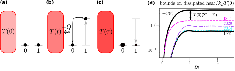
Figure 1: Landauer erasure protocol. (a) A two-level system in a maximally mixed state $\rho_{S}(0)=(|0{\rangle\langle}0|+|1{\rangle\langle}1|)/2$ with degenerate energies is in contact with a finite bath at initial temperature $T(0)$. (b) The energy of state 1 is lifted to increase the probability for a jump $1\rightarrow 0$ emitting heat $-Q$ into the bath, thereby increasing its temperature. (c) After some time $\tau$, the energy of state 1 is returned to its initial value. The final state has a population imbalance towards the state 0 (populations are indicated by the size of the black disks). (d) Plot exemplifying different inequalities in the literature for a system-bath Hamiltonian with $H_{S}=B\sigma_{S}^{z}$, $H_{B}=B\sum_{j=1}^{N}\sigma^{z}_{j}+J\sum_{j=1}^{N-1}(\sigma^{x}_{j}\sigma^{x}_{j+1}+\sigma^{y}_{j}\sigma^{y}_{j+1})$ and $V=J(\sigma^{x}_{S}\sigma^{x}_{1}+\sigma^{y}_{S}\sigma^{y}_{1})$. We chose $B=J=1$ ($\hbar\equiv 1$) and $T(0)=1/4$, see the SM for further details and plots. We plot (in logarithmic scale) the total heat $-Q(t)$ (thick black line on top) over dimensionless time $Bt$ and compare it with Landauer’s bound $-T(0)\Delta S_{S}(t)$ from 1961 Landauer (1961) (lower thick black line), the bounds from 2014 Reeb and Wolf (2014) (dotted turquoise) and 2020 Timpanaro et al. (2020) (dash-dotted purple) as well as the term $-T(0)\int_{0}^{t}{\mathchar 22\relax\mkern-12.0mud}Q(s)/T(s)$ labeled by 1865 Clausius (1865) (dashed magenta). The latter is investigated here for the first time and the difference to $-Q(t)$ is given by Eq. (4) times $T(0)$. The bound from 2015 Goold et al. (2015) is always zero for a maximally mixed initial state (see SM).

We now turn to heat engines and extend our analysis to a system in contact with a finite hot and a finite cold bath. The initial system-bath state is generalized to $\rho_{S}(0)\otimes\pi_{C}[T_{C}(0)]\otimes\pi_{H}[T_{H}(0)]$, where the subscript $C/H$ refers to the cold/hot bath.

For simplicity, we assume that the engine has operated for a sufficient amount of time (or cycles) such that its change in entropy $\Delta S_{S}$ and internal energy $\Delta U_{S}$ is negligible compared to other terms appearing in the first and second law. This is called the steady state regime and it is well justified if the system is small in comparison with the baths. However, our conclusions do not depend on this assumption as shown in the SM.

Under the conditions spelled out above, the Clausius inequality can be generalized to Strasberg and Winter (2020); Riera-Campeny et al. (2021)

$$\Sigma=-\int\frac{{\mathchar 22\relax\mkern-12.0mud}Q_{C}(t)}{T_{C}(t)}-\int\frac{{\mathchar 22\relax\mkern-12.0mud}Q_{H}(t)}{T_{H}(t)}\geq 0,$$ (7)

where ${\mathchar 22\relax\mkern-12.0mud}Q_{C/H}(t)$ denotes the infinitesimal heat flow from the baths at time $t$. Moreover, also Eq. (2) can be generalized to Esposito et al. (2010)

$$\Sigma^{\prime}=-\frac{Q_{C}(\tau)}{T_{C}(0)}-\frac{Q_{H}(\tau)}{T_{H}(0)}\geq 0.$$ (8)

The first law reads $W+Q_{C}+Q_{H}=0$ and our goal is to achieve $W<0$, i.e., we want to extract work.

Note that in presence of two baths the difference (4) is given by a sum of relative entropies, $\Sigma^{\prime}-\Sigma=D_{C}+D_{H}$ with $D_{C/H}\equiv D(\pi_{C/H}[T_{C/H}(\tau)]|\pi_{C/H}[T_{C/H}(0)])$. Hence, $\Sigma^{\prime}-\Sigma\geq 0$ still holds and it is natural to expect that a heat engine has a higher efficiency according to Eq. (7) in comparison with Eq. (8).

However, the correct definition of an efficiency for finite baths is subtle and requires some care. The standard choice $-W/Q_{H}$, which implies the Carnot bound, is adapted to the situation of an engine operating between two heat baths with a fixed temperature. This is not the case here. Instead, we argue that a meaningful efficiency can be properly defined in general as follows. Consider a positive entropy production $\Sigma$ split into two contributions labeled $A$ and $B$: $\Sigma=A+B\geq 0$. Now, the universal idea behind defining an efficiency is that we want to know how much we have to pay in order to extract something useful. Let the useful quantity be $A<0$, which has to be compensated by investing $B>0$ such that $\Sigma\geq 0$. Then, we define

$$\eta\equiv\frac{-A}{B}=1-\frac{\Sigma}{B}\leq 1.$$ (9)

Importantly, independent of $A$, $B$ and $\Sigma$, this efficiency is always bounded by the same number ($=1$). Note that our universal efficiency definition applies to any engine. This includes, e.g., also hybrid engines Manzano et al. (2020), where a similar (but not identical) efficiency was proposed.

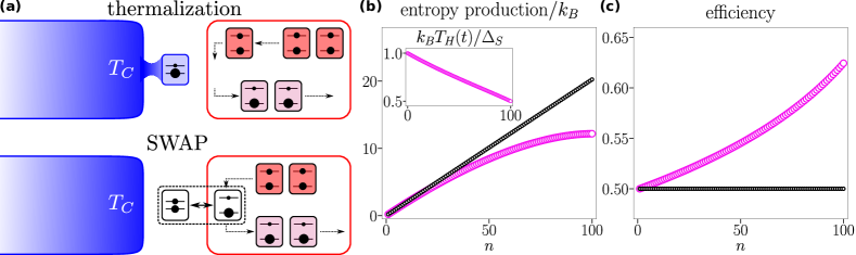
Figure 2: (a) Sketch of a system (a qubit with energy gap $\Delta_{S}$) coupled to an infinite cold bath at temperature $T_{C}$ and a finite hot bath made up of $N$ qubits with energy gap $\Delta_{H}$. The cycle of the engine consists of two steps. First, a thermalization step with the cold bath such that the system is initialized in the state $\pi_{S}(T_{C})$ (no contact with the hot bath). Second, a short and sudden interaction with a qubit of the hot bath modeled by a swap operation. Each qubit of the hot bath is initially at temperature $T_{H}(0)$, interacts only once with the system, and is afterwards found at a colder temperature (qubit populations are indicated by the size of the black disks). The model is exactly solved in the SM and work extraction is possible if $\Delta_{S}/\Delta_{H}>T_{C}/T_{H}(0)$. (b) We plot $\Sigma$ (large magenta circles) and $\Sigma^{\prime}$ (small black circles) and the changing temperature $T_{H}(t)$ of the finite hot bath (inset) as a function of the number of cycles $n$ for $N=100$ qubits in the hot bath. (c) Plot of $\eta$ (large magenta circles) and $\eta^{\prime}$ (small black circles) as a function of $n$. All our plots confirm our conclusions in the main text. Numerical parameters: $\Delta_{S}=1$, $\Delta_{H}=3/2$, $T_{H}(0)=1$, $T_{C}=1/3$.

We start by applying this logic to $\Sigma^{\prime}$. Using the first law, we rewrite Eq. (8) as

$$\Sigma^{\prime}=\frac{W(\tau)}{T_{C}(0)}+\frac{Q_{H}(\tau)}{T_{C}(0)}-\frac{Q_{H}(\tau)}{T_{H}(0)}\geq 0.$$ (10)

Clearly, if operated as a heat engine, the first term is negative and we identify $A^{\prime}=W(\tau)/T_{C}(0)$, whereas $B^{\prime}=\eta_{C}[T_{C}(0),T_{H}(0)]Q_{H}(\tau)/T_{C}(0)$ is then necessarily positive. Here, we defined the Carnot efficiency $\eta_{C}(T_{C},T_{H})\equiv 1-T_{C}/T_{H}$. Then, we find

$$\eta^{\prime}=\frac{-A^{\prime}}{B^{\prime}}=\frac{1}{\eta_{C}[T_{C}(0),T_{H}(0)]}\frac{-W(\tau)}{Q_{H}(\tau)}\leq 1,$$ (11)

which simply is a linearly rescaled version of the conventional definition.

Next, we apply this logic to $\Sigma$ and write $\Sigma=A+B$. Now, to make a comparison of efficiencies meaningful, we define them with respect to the same useful quantity $A=A^{\prime}=W(\tau)/T_{C}(0)$. However, the $B$-term is now different because the resources invested in order to extract $A$ are differently counted. Specifically, we find

$$\begin{split}B=&\int\frac{{\mathchar 22\relax\mkern-12.0mud}Q_{C}(t)}{T_{C}(0)}\eta_{C}[T_{C}(0),T_{C}(t)]\\ &+\int\frac{{\mathchar 22\relax\mkern-12.0mud}Q_{H}(t)}{T_{C}(0)}\eta_{C}[T_{C}(0),T_{H}(t)],\end{split}$$ (12)

which quantifies a rescaled heat dissipation. In the limit of constant bath temperatures, $T_{C/H}(t)=T_{C/H}(0)$, we obtain $B=B^{\prime}$. More interestingly, using $\eta=-A/B$, our central result (4) allows us to conclude

$$\eta^{\prime}=\left(1-\frac{T_{C}(0)(D_{C}+D_{H})}{\eta_{C}[T_{C}(0),T_{H}(0)]Q_{H}(\tau)}\right)\eta\leq\eta.$$ (13)

We recapitulate our logic used to arrive at the general conclusion $\eta\geq\eta^{\prime}$. We started from two different inequalities $\Sigma\geq 0$ and $\Sigma^{\prime}\geq 0$. In both inequalities, the same microsopically defined heat and work fluxes enter, but they are bounded in different ways. Based on these two inequalities, we constructed two efficiencies $\eta$ and $\eta^{\prime}$. Importantly, (i) these efficiencies are both bounded by 1 and (ii) both quantify the amount of resources needed to extract the same quantity $A=W/T_{C}(0)$. They are therefore comparable and we have shown in full generality that $\eta\geq\eta^{\prime}$ arises as a consequence of $\Sigma^{\prime}\geq\Sigma$. We also add that, instead of fixing the extracted resources $A=A^{\prime}$ to be the same [condition (ii)], we could likewise fix the invested resources $B=B^{\prime}$. It is easy to check that our conclusion remains: $\eta\geq\eta^{\prime}$.

To illustrate the above points, we have numerically simulated a heat engine in contact with an infinite cold bath and a finite hot bath. Our setup combines the idea of a swap engine Campisi et al. (2015) with the framework of repeated interactions Strasberg et al. (2017) and is explained in detail in Fig. 2 and the SM. Our numerical observations in Fig. 2 confirm our general claims. For other studies of heat engines in contact with finite baths see Refs. Brandner et al. (2015); Brandner and Seifert (2016); Brandner and Saito (2020); Izumida and Okuda (2014); Wang (2016); Pozas-Kerstjens et al. (2018).

Before concluding, we emphasize another subtle point. We stressed above that Clausius’ inequality is identical to the change in thermodynamic entropy of the universe for an ideal heat bath, which is well described by a macroscopic temperature $T(t)$. However, via definition (3), Eq. (1) remains microscopically valid for any bath state, but in this case $-{\mathchar 22\relax\mkern-12.0mud}Q(t)/T(t)$ no longer strictly relates to a change in bath entropy. Remarkably, it is possible to generalize the second law to also account for information about the (coarse-grained) distribution of bath energies Strasberg and Winter (2020); Riera-Campeny et al. (2021). For the same reasons as explained below Eq. (4), the corresponding efficiency with respect to this refined second law is even higher than $\eta$, which we show explicitly in the SM. Thus, having access to further information in form of the nonequilibrium distribution of bath energies offers additional interesting benefits in unison with other recent findings Hajiloo et al. (2020). Note, however, that the present approach relies arguably only on the minimal information required; namely, the average bath energy $E_{B}(\tau)$ or (which is in one-to-one correspondence) its temperature $T(\tau)$.

To conclude, 155 years ago, Clausius wrote down a remarkable inequality, which remained unappreciated in quantum thermodynamics. Here, we emphasized that the original Clausius inequality (1) correctly quantifies the second law for a much larger class of situations than the conventionally employed inequality (2). We showed that Eq. (1) can be fruitfully used to study nanomachines in contact with finite baths and, importantly, it is easy to apply in computations as it only relies on the knowledge of the bath energy. Whether it is simple to experimentally measure the bath energy depends on the platform. Here, it could be helpful to develop thermometry schemes Mehboudi et al. (2019), which are adapted to the nonequilibrium temperature defined in Eq. (3). Finally and most remarkably, the ancient Clausius inequality offers the insight that nanoscale engines are more efficient than previously anticipated.

Acknowledgements.—We are grateful to Anna Sanpera for many stimulating discussions and valuable comments on the manuscript. PS is financially supported by the DFG (project STR 1505/2-1). MGD acknowledges financial support from Secretaria d’Universitats i Recerca del Departament d’Empresa i Coneixement de la Generalitat de Catalunya, co-funded by the European Union Regional Development Fund within the ERDF Operational Program of Catalunya (project QuantumCat, ref. 001-P-001644). ARC acknowledges financial support from the Generalitat de Catalunya: AGAUR FI2018-B01134. All authors acknowledge financial support from the Spanish Agencia Estatal de Investigación, project PID2019-107609GB-I00, the Spanish MINECO FIS2016-80681-P (AEI/FEDER, UE), and Generalitat de Catalunya CIRIT 2017-SGR-1127.

Appendix A SUPPLEMENTARY MATERIAL

We here detail in chronological order additional information concerning (A) the derivation of Eq. (4) in the maintext, (B) the Landauer erasure protocol used for the numerics, (C) the swap engine coupled to a repeated interactions bath, (D) the fact that our conclusions remain true even if the system has not yet reached a steady state, (E) improved efficiencies if additional information about the nonequilibrium probability distribution of the bath energies is available. Here, we sometimes make use of the inverse temperature $\beta(t)=1/T(t)$ whenever convenient.

Appendix B (A) Details concerning the derivation of Eq. (4) in the maintext

We formulate our derivation using the inverse temperature $\beta(t)$ and assume for the moment that it changes in a differentiable way. We start by considering the integral

$$-\int\frac{{\mathchar 22\relax\mkern-12.0mud}Q(t)}{T(t)}=\int_{0}^{\tau}dt\beta(t)\frac{dE_{B}(t)}{dt},$$ (14)

where we used $-{\mathchar 22\relax\mkern-12.0mud}Q(t)=dE_{B}(t)=\mbox{tr}_{B}\{H_{B}[\rho_{B}(t+dt)-\rho_{B}(t)]\}$. The next step requires to confirm that

$$\frac{dE_{B}(t)}{dt}=-\dot{\beta}(t)\mbox{Var}[H_{B},\beta(t)],\leavevmode\nobreak\ \leavevmode\nobreak\ \leavevmode\nobreak\ \dot{\beta}(t)\equiv\frac{d\beta(t)}{dt},\leavevmode\nobreak\ \leavevmode\nobreak\ \leavevmode\nobreak\ \mbox{Var}(H_{B},\beta)\equiv\mbox{tr}_{B}\{H_{B}^{2}\pi_{B}(\beta)\}-\mbox{tr}_{B}\{H_{B}\pi_{B}(\beta)\}^{2}.$$ (15)

Note that the first equation in Eq. (15) is equivalent to the known result for the heat capacity of the canonical ensemble, $C_{B}\equiv dE(t)/dT(t)=\mbox{Var}[H_{B},\beta(t)]/T(t)^{2}$, after noting that $\dot{\beta}(t)=-\dot{T}(t)/T(t)^{2}$.

Now, let $S_{B}(\beta)\equiv-\mbox{tr}_{B}\{\pi_{B}(\beta)\ln\pi_{B}(\beta)\}$ denote the von Neumann entropy of a canonical equilibrium state at inverse temperature $\beta$. Using $d_{t}S_{\text{vN}}[\rho(t)]=-\mbox{tr}\{[d_{t}\rho(t)]\ln\rho(t)\}$ and manipulations similar to those required to obtain Eq. (15), we find that

$$\frac{dS_{B}[\beta(t)]}{dt}=-\beta(t)\dot{\beta}(t)\mbox{Var}[H_{B},\beta(t)].$$ (16)

Taken together, we confirm that

$$\int_{0}^{\tau}dt\beta(t)\frac{dE_{B}(t)}{dt}=\int_{0}^{\tau}dt\frac{dS_{B}[\beta(t)]}{dt}=S_{B}[\beta(\tau)]-S_{B}[\beta(0)].$$ (17)

Next, we note the general identity

$$-\frac{Q(\tau)}{T(0)}=\mbox{tr}_{B}\{\pi_{B}[\beta(0)]\ln\pi_{B}[\beta(0)]\}-\mbox{tr}_{B}\{\pi_{B}[\beta(\tau)]\ln\pi_{B}[\beta(0)]\}.$$ (18)

Combining this with Eq. (17), we confirm

$$\Sigma^{\prime}-\Sigma=-\frac{Q(\tau)}{T_{0}}+\int_{0}^{\tau}\frac{{\mathchar 22\relax\mkern-12.0mud}Q(t)}{T(t)}=D\big{[}\pi_{B}[\beta(\tau)]\left|\pi_{B}[\beta(0)]\big{]}\right.,$$ (19)

which proves Eq. (4) in the maintext of the main text.

Two comments are important. First, we preferred to work with $\beta(t)$ instead of $T(t)$. This choice is related to the phenomenon that for a bath with a finite Hilbert space (note that there can be finite baths with an infinite Hilbert space, e.g., a collection of particles in a box) the temperature $T(t)$ becomes negative for a population inverted state. Importantly, when the state changes continuously from a state $\rho_{B}(t_{-})$ without population inversion to a state $\rho_{B}(t_{+})$ with population inversion, the associated temperature $T(t)$ changes via definition (3) in the maintext from $T(t_{-})=\infty$ to $T(t_{+})=-\infty$, i.e., there is a sudden and discontinuous jump in the temperature. However, this jump can be avoided when working with the inverse temperature, which changes continuously from $\beta(t_{-})>0$ to $\beta(t_{+})<0$. Therefore, by working with the inverse temperature, we demonstrated that our conclusions remain true even for exotic negative temperature states in the bath.

Second, we comment on the assumption that $\beta(t)$ needs to be differentiable. In fact, since unitary dynamics generated by the Liouville-von Neumann equation are differentiable, there are good reasons to expect that the effective (inverse) temperature of the bath defined via Eq. (3) in the maintext also changes in a differentiable way. Importantly, since the relation $dS_{B}[\beta(t)]=\beta(t)dE_{B}[\beta(t)]$ has to hold only under the integral, our central result (4) in the maintext remains valid if there is a finite number of times for which $\beta(t)$ is not differentiable, but still continuous. We indeed observe this behaviour in Sec. (B), where $\beta(t)$ shows (non-differentiable) spikes without invalidating Eq. (4) in the maintext. Finally, cases where $\beta(t)$ is not even continuous can be only generated by singular cases such as, e.g., a Hamiltonian with a time-dependence described by a Dirac delta function. Strictly speaking, these models are, of course, unphysical. Nevertheless, we investigate this case in detail in Sec. (C) for the swap engine. Indeed, the swap engine models the swap operation as happening instantaneously, which generates a discontinuous evolution of $\beta(t)$. Despite this feature, we find that the central inequality $\Sigma^{\prime}-\Sigma\geq 0$ continuous to hold and that the difference between $\Sigma^{\prime}-\Sigma$ and $D\{\pi_{B}[\beta(\tau)]|\pi_{B}[\beta(0)]\}$ quickly becomes negligibly small.

Appendix C (B) Details of the Landauer erasure protocol

We first review the bounds of Refs. Reeb and Wolf (2014); Goold et al. (2015); Timpanaro et al. (2020) before specifying the details of our numerical studies.

C.1 Bounds to the dissipated heat

The bound of Ref. Reeb and Wolf (2014) reads

$$-Q(\tau)\geq-T(0)\Delta S_{S}(\tau)+\frac{2T(0)\Delta S_{S}^{2}(\tau)}{\ln^{2}(d-1)+4},$$ (20)

where $d$ is the dimension of the bath Hilbert space.

The bound of Ref. Goold et al. (2015) is based on the fact that the dynamics of the bath can be written as $\rho_{B}(t)=\sum_{\alpha}A_{\alpha}(t)\rho_{B}(0)A_{\alpha}^{\dagger}(t)$, where the bath operators $A_{\alpha}(t)$ are commonly called Kraus operators. Defining $\textbf{A}(t)\equiv\sum_{\alpha}A_{\alpha}(t)A_{\alpha}^{\dagger}(t)$, the bound reads

$$-Q(t)\geq-T(0)\ln\mbox{tr}_{B}\{\textbf{A}(t)\rho_{B}(0)\}.$$ (21)

We now demonstrate that this bound is zero for the case of Landauer erasure, i.e., whenever the system starts in a maximally mixed state. To this end, we note that the operators $A_{\alpha}(t)$ are microscopically defined as $A_{\alpha}(t)=\sqrt{\lambda_{j}}\langle s_{k}|U_{SB}(t)|s_{j}\rangle$, where $U_{SB}(t)$ is the global system bath unitary and the initial state of the system was decomposed as $\rho_{S}(0)=\sum_{j}\lambda_{j}|s_{j}{\rangle\langle}s_{j}|$. Thus, we see that the index $\alpha$ is actually a double-index $\alpha=(j,k)$. Now, if $\rho_{S}(0)$ is a maximally mixed state, then $\lambda_{j}=1/\sqrt{d_{S}}$, where $d_{S}$ is the dimension of the system Hilbert space. Consequently,

$$\textbf{A}(t)=\sum_{\alpha}A_{\alpha}(t)A_{\alpha}^{\dagger}(t)=\sum_{j,k}\frac{1}{d_{S}}\langle s_{k}|U_{SB}(t)|s_{j}\rangle\langle s_{j}|U_{SB}^{\dagger}(t)|s_{k}\rangle=\sum_{k}\frac{1}{d_{S}}\langle s_{k}|U_{SB}(t)U_{SB}^{\dagger}(t)|s_{k}\rangle=\sum_{k}\frac{1}{d_{S}}=1,$$ (22)

where $1$ denotes the identity operator in the bath space. Thus, $-\ln\mbox{tr}_{B}\{\textbf{A}(t)\rho_{B}(0)\}=-\ln(1)=0$.

Next, we turn to the bound from Ref. Timpanaro et al. (2020). Interestingly, this bound also employs the temperature definition (3) in the maintext. We introduce the two functions $f[\beta(t)]\equiv\mbox{tr}_{B}\{H_{B}\pi_{B}[\beta(t)]\}-\mbox{tr}_{B}\{H_{B}\pi_{B}[\beta(0)]\}$ and $g[\beta(t)]\equiv S_{B}[\beta(t)]-S_{B}[\beta(0)]$, which determine the energy and entropy change with respect to the fictitious equilibrium state of the bath at inverse temperature $\beta(t)$ starting from $\beta(0)$. It was then found that

$$-Q(t)\geq(f\circ g^{-1})[-\Delta S_{S}(t)].$$ (23)

Here, $(f\circ g^{-1})(x)\equiv f[g^{-1}(x)]$ denotes the concatenation of two functions.

C.2 Model 1: Spin coupled to a spin chain

The total system-bath Hamiltonian $H_{S}+H_{B}+V$ is specified by

$$H_{S}=B_{0}\sigma_{z}^{S},\leavevmode\nobreak\ \leavevmode\nobreak\ \leavevmode\nobreak\ H_{B}=B\sum_{j=1}^{N}\sigma_{z}^{(j)}+J\sum_{j=1}^{N-1}(\sigma_{x}^{(j)}\sigma_{x}^{(j+1)}+\sigma_{y}^{(j)}\sigma_{y}^{(j+1)}),\leavevmode\nobreak\ \leavevmode\nobreak\ \leavevmode\nobreak\ V=J_{0}(\sigma_{x}^{S}\sigma_{x}^{(1)}+\sigma_{y}^{S}\sigma_{y}^{(1)}).$$ (24)

Here, $\sigma_{x,y,z}$ denotes the usual Pauli matrix, $N$ the number of spins in the bath and $B_{0},B,J_{0}$ and $J$ are real-valued parameters. The time-evolution of the system-bath state is implemented by exact numerical integration.

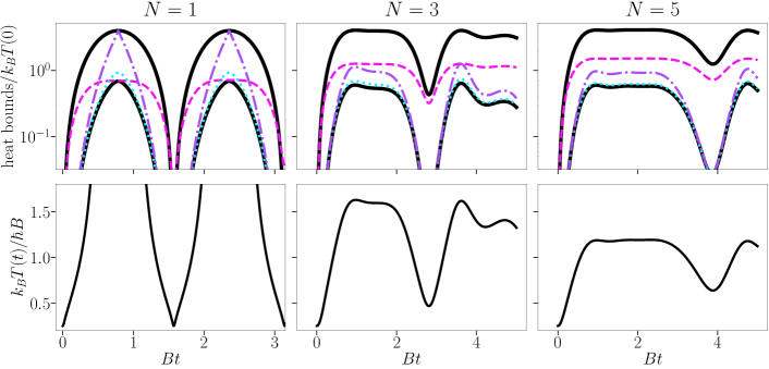
Figure 3: First row: As a function of dimensionless time $Bt$ for $N=1$ (left), $N=3$ (center) and $N=5$ (right) spins in the bath, plot of the dissipated heat $-Q(t)$ and Landauer’s original lower bound $-T(0)\Delta S_{S}(t)$ (thick solid black lines) and the bound (20) Reeb and Wolf (2014) (dotted turquoise line), the bound (23) Timpanaro et al. (2020) (dash-dotted purple line) and our bound (6) in the maintext (dashed magenta line). Note that we used a logarithmic scale for better visibility. Second row: Again as a function of time for $N=1$ (left), $N=3$ (center) and $N=5$ (right) spins in the bath, plot of the time-evolution of the (dimensionless) nonequilibrium temperature $T(t)$. Numerical parameters: $B=B_{0}=1$, $J=J_{0}=1$, $T(0)=1/4$.

We start by giving additional numerical results concering the Landauer erasure protocol, which starts with a maximally mixed state $\rho_{S}(0)=(|0{\rangle\langle}0|+|1{\rangle\langle}1|)/2$, where $|0\rangle$ ($|1\rangle$) denotes the ground (excited) state of the system. Figure 3 shows the bounds from Refs. Landauer (1961); Reeb and Wolf (2014); Timpanaro et al. (2020) and our bound (6) in the maintext on the total heat dissipation for $N=1,3,5$ spins in the bath. We observe that there is no particular order between our bound and the bounds from Refs. Reeb and Wolf (2014); Timpanaro et al. (2020). Furthermore, for $N=1$ we observe non-differentiable ‘spikes’ in the evolution of the temperature $T(t)$. Nevertheless, in unison with our last comment in Sec. (A), we find perfect agreement with our central result (4) in the maintext (not shown explicitly).

Next, we provide additional numerical results when the system starts in a pure state, which we take to be the excited state. In this case, we expect the bound from Ref. Goold et al. (2015) to be useful and, indeed, Fig. 4 demonstrates this. Furthermore, Fig. 4 illustrates two additional insights. First, for $N=1$ the bound of Ref. Timpanaro et al. (2020) does not exist for all times since the image of the function $g$ in Eq. (23) is not guaranteed to contain the value $-\Delta S_{S}(t)$. Second, instead of plotting the temperature of the bath in the second row, we plot its inverse temperature. In fact, for $N=1$ the temperature switches from a positive to a negative value during the evolution, which would result in discontinuous jumps in $T(t)$ from $\infty$ to $-\infty$, whereas $\beta(t)$ behaves smoothly changes from $0^{+}$ to $0^{-}$.

We remark that we have not performed an exhaustive numerical study, but for all the parameters we checked we found numerically the same qualitative behaviour. This is also confirmed by our next model.

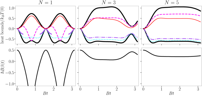
Figure 4: As a function of dimensionless time $Bt$ for $N=1$ (left), $N=3$ (center) and $N=5$ (right) spins in the bath, plot of the dissipated heat $-Q(t)$ and Landauer’s original lower bound $-T(0)\Delta S_{S}(t)$ (thick solid black lines) and the bound (20) Reeb and Wolf (2014) (dotted turquoise line), the bound (21) Goold et al. (2015) (thin red solid line), the bound (23) Timpanaro et al. (2020) (dash-dotted purple line, except for $N=1$ where the bound only exists for a subset of times and where we used a thick purple line) and our bound (6) in the maintext (dashed magenta line). Parameters are as in Fig. 3 except of a different temperature, $T(0)=2$, and a different initial system state (an excited state).

C.3 Model 2: Spin coupled to a random matrix environment

This model was investigated in detail in Sec. IV of Ref. Riera-Campeny et al. (2021). It also consists of a spin with Hamiltonian $H_{S}=\epsilon_{0}|0{\rangle\langle}0|+\epsilon_{1}|1{\rangle\langle}1|$ in contact with a bath with Hamiltonian $H_{B}=\sum_{j}E_{j}|j{\rangle\langle}j|$. The bath Hamiltonian is split into two energy bands ${\cal{E}}_{0}$ and ${\cal{E}}_{1}$. Each band ${\cal{E}}_{i}$ is of width $\delta$ centered around $\epsilon_{i}$ and contains a number of $V_{i}$ eigenenergies, which are randomly sampled from the interval $[\epsilon_{i}-\delta/2,\epsilon_{i}+\delta/2)$. Furthermore, we assume $\epsilon_{1}-\epsilon_{0}\geq\delta$ such that the two bands do not overlap. For the numerics, we set $V_{0}=10$ and leave $V\equiv V_{1}$ as a free parameter. Finally, the interaction Hamiltonian is

$$V=\lambda\sigma_{x}\otimes B,\leavevmode\nobreak\ \leavevmode\nobreak\ \leavevmode\nobreak\ B=\sum_{E_{j}\in{\cal{E}}_{0}}\sum_{E_{k}\in{\cal{E}}_{1}}c(E_{j},E_{k})|E_{j}{\rangle\langle}E_{k}|+\text{h.c.}$$ (25)

Here, $c(E_{j},E_{k})$ is a matrix of independent and identically distributed complex random numbers with zero mean and variance $a^{2}$. The dynamics are generated by formally integrating the exact Schrödinger dynamics for one realization of the coupling matrix $c(E_{j},E_{k})$, but we observe that the qualitative features of the dynamics do not change for different realizations. Despite the bath dimension $d=V_{0}+V_{1}=10+V$ is relatively small, the randomness in the coupling helps to mimic a more realistic (i.e., large) heat bath. Numerical results are shown in Fig. 5 for the case of Landauer erasure.

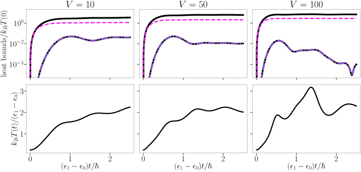
Figure 5: First row: As a function of dimensionless time $(\epsilon_{1}-\epsilon_{0})t/\hbar$ for $V=10$ (left), $V=50$) (center) and $V=100$ (right) levels in the upper band of the bath, plot of the dissipated heat $-Q(t)$ and Landauer’s original lower bound $-T(0)\Delta S_{S}(t)$ (thick solid black lines) and the bound (20) Reeb and Wolf (2014) (dotted turquoise line), the bound (23) Timpanaro et al. (2020) (dash-dotted purple line) and our bound (6) in the maintext (dashed magenta line). Note that we used a logarithmic scale for better visibility. Second row: Again as a function of dimensionless time for $V=10$ (left), $V=50$) (center) and $V=100$ (right) levels in the upper band of the bath, plot of the time-evolution of the (dimensionless) nonequilibrium temperature $T(t)$. Numerical parameters: $\epsilon_{1}-\epsilon_{0}=1$, $\delta=1$, $\lambda=0.3$, $T_{0}=1/4$.

Appendix D (C) The swap engine with a repeated interactions bath

We consider a two-level system with Hamiltonian $H_{S}=\Delta_{S}|1{\rangle\langle}1|$, where $|1\rangle$ denotes the excited state (and $|0\rangle$ the ground state) as our ‘working medium’.

The cold bath is assumed to be an ideal weakly coupled bath, which simply prepares the system in a canonical ensemble at temperature $T_{C}$ in each cycle. We denote this state as $\pi_{S}(T_{C})\equiv e^{-H_{S}/T_{C}}/{\cal{Z}}_{S}(t_{C})$.

The hot bath is made up of $N$ non-interacting qubits. Each qubit is described by the Hamiltonian $H_{H}=\Delta_{H}|1{\rangle\langle}1|$ and initialized in the state $\pi_{H}[T_{H}(0)]=e^{-H_{H}/T_{H}(0)}/{\cal{Z}}_{H}[T_{H}(0)]$. At regular time-intervals $k\tau_{\text{cycle}}$, the $k$’th qubit of the hot bath interacts with the system. This interaction is assumed to be fast enough such that the effect of the cold bath can be neglected to lowest order. Furthermore, we assume the time $\tau_{\text{cycle}}$ between two interaction to be large enough such that the system had enough time to relax to the thermal state $\pi_{S}(T_{C})$ in between two interactions. Finally, we assume that the interaction between the $k$’th bath qubit and the system implements a swap operation described via the unitary operator $U_{\text{swap}}|k,l\rangle=|l,k\rangle$. Here, $|k,l\rangle=|k\rangle_{S}\otimes|l\rangle_{H}$ denotes the system qubit in state $k$ and the bath qubit in state $l$ ($k,l\in\{0,1\}$).

We are now in a position, where we can analyze an arbitrary cycle from a thermodynamic perspective. We start with the swap operation. The total work equals the change in internal energy of the system and the bath qubit:

$$W=\mbox{tr}_{SB}\{(H_{S}+H_{B})[U_{\text{swap}}\pi_{S}(T_{C})\otimes\pi_{H}[T_{H}(0)]U_{\text{swap}}^{\dagger}-\pi_{S}(T_{C})\otimes\pi_{H}[T_{H}(0)]]\}.$$ (26)

Since there is no work performed on the system during the thermalization processes, we want that this work is negative. A quick calculation reveals the explicit expression

$$W=(\Delta_{S}-\Delta_{H})\left[\frac{e^{-\Delta_{H}/T_{H}(0)}}{{\cal{Z}}_{H}[T(0)]}-\frac{e^{-\Delta_{S}/T_{C}}}{{\cal{Z}}_{S}(T_{C})}\right]=(\Delta_{S}-\Delta_{H})\frac{e^{\Delta_{S}/T_{C}}-e^{\Delta_{H}/T_{H}(0)}}{(e^{\Delta_{H}/T_{H}(0)}+1)(e^{\Delta_{S}/T_{C}}+1)}.$$ (27)

The condition for work extraction, $W<0$, follows as

$$\frac{T_{H}(0)}{T_{C}}>\frac{\Delta_{H}}{\Delta_{S}}>1.$$ (28)

From Eq. (26) we can also easily calculate the change in system and bath energy during the swap operation, which becomes

$$\Delta E_{S}=\Delta_{S}\left[\frac{e^{-\Delta_{H}/T_{H}(0)}}{{\cal{Z}}_{H}[T(0)]}-\frac{e^{-\Delta_{S}/T_{C}}}{{\cal{Z}}_{S}(T_{C})}\right],\leavevmode\nobreak\ \leavevmode\nobreak\ \leavevmode\nobreak\ \Delta E_{H}=-\frac{\Delta_{H}}{\Delta_{S}}\Delta E_{S}=-Q_{H}.$$ (29)

Here, we equated the change in bath energy with minus the heat flow into it in accordance with our framework above and we observe that $W=\Delta E_{S}-Q_{H}$, which is the first law during the swap operation.

During the subsequent equilibration step, the system relaxes back to its initial state by dissipating an amount of heat $Q_{C}=-\Delta E_{S}$ into the cold bath. This concludes the cycle. Note that the system entropy and energy does not change over an entire cycle, a property which we also used in the main text.

Now, the total amount of heat flown and the work after $n$ interactions simply become

$$Q_{H}^{\text{tot}}=nQ_{H},\leavevmode\nobreak\ \leavevmode\nobreak\ \leavevmode\nobreak\ Q_{C}^{\text{tot}}=nQ_{C},\leavevmode\nobreak\ \leavevmode\nobreak\ \leavevmode\nobreak\ W^{\text{tot}}=nW=-Q_{C}^{\text{tot}}-Q_{H}^{\text{tot}}.$$ (30)

Furthermore, the two different notions of entropy production become after $n$ interactions

$$\Sigma=-\frac{nQ_{C}}{T_{C}}-\sum_{k=1}^{n}\frac{Q_{H}}{T_{H}(k\tau)}\geq 0,\leavevmode\nobreak\ \leavevmode\nobreak\ \leavevmode\nobreak\ \Sigma^{\prime}=-\frac{nQ_{C}}{T_{C}}-\frac{nQ_{H}}{T_{H}(0)}\geq 0,$$ (31)

which is plotted in Fig. 2(b). Furthermore, the time-dependent temperature of the hot bath $T_{H}(k\tau)$, which is plotted in the inset of Fig. 2(b), can be obtained by solving

$$k\frac{\Delta_{H}}{e^{\Delta_{S}/T_{C}}+1}+(N-k)\frac{\Delta_{H}}{e^{\Delta_{H}/T_{H}(0)}+1}=N\frac{\Delta_{H}}{e^{\Delta_{H}/T_{H}(k\tau)}+1},$$ (32)

where $N$ denotes the total number of qubits in the hot bath. Note that for $k=N$ the temperature of the finite bath is exactly $T_{H}(N\tau)=T_{C}\Delta_{H}/\Delta_{S}$. According to Eq. (28), this means that we can no longer extract work from the system after we have used up all $N$ qubits. The plot of the efficiencies $\eta$ and $\eta^{\prime}$, Fig. 2(c), immediately follows from the above considerations.

Finally, we return to the second comment made at the end of Sec. (A) of the SM. There, we found that our central result (4) in the maintext can break down if the bath temperature does not change in a differentiable way, which is the case here. Clearly, this behaviour is the more pronounced, the smaller the number of qubits in the cold bath. In the extreme case of a bath with a single qubit, the temperature would instantaneously jump from $T_{H}(0)$ to $T_{H}(\tau)=T_{C}\Delta_{H}/\Delta_{S}<T_{H}(0)$. Once more, we repeat that this behaviour is unphysical. In reality, the implementation of the swap operation takes a finite time and then $T_{H}(t)$ would change continuously.

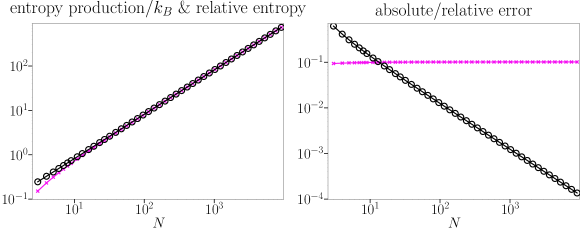
Figure 6: Left: Plot of $\Sigma^{\prime}(N)-\Sigma(N)$ (pink crosses) and $ND[\pi_{B}[T_{H}(N\tau)]|\pi_{B}[T_{H}(0)]]$ (black circles) as a function of $N$. Right: Plot of $e_{\text{abs}}(N)$ (pink crosses) and $e_{\text{rel}}(N)$ (black circles) as a function of $N$. Note that in both plots results are shown on a double-logarithmic scale. Numerical parameters are as for Fig. 2 in the main text: $\Delta_{S}=1$, $\Delta_{H}=3/2$, $T_{H}(0)=1$, $T_{C}=1/3$.

Out of curiosity, we ask, however, what happens to our central result (4) in the maintext for the idealized swap engine considered here. The answer is shown in Fig. 6, where we plot the following quantities. First, we plot $\Sigma^{\prime}(N)-\Sigma(N)$ as a function of the number of qubits $N$ in the hot bath after $N$ cycles have been completed (i.e., after each bath qubit has interacted with the system). As one can see (left plot in Fig. 6), the inequality $\Sigma^{\prime}(N)-\Sigma(N)\geq 0$ continuous to hold. Next, in the same plot we also show the relative entropy between the initial state of the hot bath at temperature $T_{H}(0)$ and the associated final equilibrium state at $T_{H}(\tau)$. Since there are no correlations between the qubits in the hot bath, this quantity becomes $ND\{\pi_{B}[T_{H}(\tau)]|\pi_{B}[T_{H}(0)]\}$, where $\pi_{B}(T)$ is the canonical ensemble at temperature $T$ of a single qubit. We observe that, in unison with our central result (4) in the maintext, the disagreement with $\Sigma^{\prime}(N)-\Sigma(N)$ is very small already for moderate $N$. To quantify this difference more precisely, we also display the absolute and relative error in the right plot of Fig. 6:

$$e_{\text{abs}}(N) \equiv\Sigma^{\prime}(N)-\Sigma(N)-ND[\pi_{B}[T_{H}(N\tau)]|\pi_{B}[T_{H}(0)]],$$ (33)

$$e_{\text{rel}}(N) \equiv\frac{\Sigma^{\prime}(N)-\Sigma(N)-ND[\pi_{B}[T_{H}(N\tau)]|\pi_{B}[T_{H}(0)]]}{\Sigma^{\prime}(N)-\Sigma(N)}.$$ (34)

While the absolute error stays constant as a function of $N$, the relative error decreases as $1/N$ because the ‘amount of discontinuity’ in $T_{H}(t)$ gets smaller with increasing $N$. This result is intuitive and reassuring.

Appendix E (D) Nanoscopic heat engines beyond the steady state regime

If the system has not yet reached a steady state, Eqs. (7) in the maintext and (8) in the maintext of the main text generalize to

$$\Sigma =\Delta S_{S}(\tau)-\int\frac{{\mathchar 22\relax\mkern-12.0mud}Q_{C}(t)}{T_{C}(t)}-\int\frac{{\mathchar 22\relax\mkern-12.0mud}Q_{H}(t)}{T_{H}(t)}\geq 0,$$ (35)

$$\Sigma^{\prime} =\Delta S_{S}(\tau)-\frac{Q_{C}(\tau)}{T_{C}(0)}-\frac{Q_{H}(\tau)}{T_{H}(0)}\geq 0.$$ (36)

Using the first law $\Delta U_{S}=Q_{C}+Q_{H}+W$, we can rewrite both expressions as

$$\Sigma^{\prime}=\frac{W(\tau)}{T_{C}(0)}-\frac{\Delta F_{S}(\tau)}{T_{C}(0)}+\frac{Q_{H}(\tau)}{T_{C}(0)}-\frac{Q_{H}(\tau)}{T_{H}(0)}\geq 0.$$ (37)

Here, we have introduced the change in nonequilibrium free energy $\Delta F_{S}(\tau)=\Delta U_{S}(\tau)-T_{C}(0)\Delta S_{S}(\tau)$ with respect to the reference temperature $T_{C}(0)$ of the initial cold bath. Now, there are different possibilities to split $\Sigma^{\prime}$ into an $A$- and $B$-term depending on which resources we want to convert to each other. However, independent of how we split $\Sigma^{\prime}=A+B$, we can always write

$$\Sigma=A+B+\Sigma-\Sigma^{\prime}.$$ (38)

Therefore, we obtain the efficiencies

$$\eta^{\prime}=\frac{-A}{B},\leavevmode\nobreak\ \leavevmode\nobreak\ \leavevmode\nobreak\ \eta=\frac{-A}{B+\Sigma-\Sigma^{\prime}}.$$ (39)

Since $0<B+\Sigma-\Sigma^{\prime}\leq B$, we obtain in general the conclusion that $\eta^{\prime}/\eta\leq 1$. Thus, for any process (not just heat engines) the true efficiency according to the second law (1) in the maintext is larger than the efficiency inferred from Eq. (2) in the maintext, which was previously asserted to be the second law Binder et al. (2018); Landi and Paternostro (2020).

Appendix F (E) Efficiencies and second law for far-from-equilibrium baths

In general, a finite bath might be driven out of equilibrium during a thermodynamic process such that it is no longer well described by a time-dependent temperature (although this does not seem to be the case in most current experiments Trotzky et al. (2012); Brantut et al. (2012); Gring et al. (2012); Brantut et al. (2013); Clos et al. (2016); Kaufman et al. (2016); Karimi et al. (2020)). In order to describe the bath more accurately, we then need, however, more information. Here, we assume this information to be available in terms of the probability distribution of the bath energies $p(e_{B},t)$ at time $t$ (we only consider one bath here, but the argument generalizes to multiple baths). Here, $e_{B}$ does not necessarily refer to an eigenenergy of the bath Hamiltonian. Instead, $p(e_{B},t)$ can describe some coarse-grained probability distribution as long as the error is small enough such that, for instance, the average bath energy is well approximated by

$$\mbox{tr}_{B}\{H_{B}\rho_{B}(t)\}\approx\sum_{e_{B}}e_{B}p(e_{B},t).$$ (40)

Since $e_{B}$ does not necessarily refer to a single energy eigenstate, we denote by $V(e_{B})$ all microstates which give rise to measurement outcome $e_{B}$. Note, if $p(e_{B},t)=\delta_{e_{B},e^{\prime}_{B}}$ for some $e^{\prime}_{B}$, then the state of the bath equals the conventional microcanonical ensemble.

We now define the following notion of entropy, which is known as observational entropy (for a recent review of this concept, which goes back to Boltzmann, Gibbs, von Neumann and Wigner, see Ref. Šafránek et al. (2020)):

$$S_{\text{obs}}^{E_{B}}(t)\equiv\sum_{e_{B}}p(e_{B},t)[-\ln p(e_{B},t)+\ln V(e_{B})].$$ (41)

As demonstrated in Refs. Strasberg and Winter (2020); Riera-Campeny et al. (2021), the second law can then be generalized to

$$\tilde{\Sigma}=\Delta S_{S}(\tau)+S_{\text{obs}}^{E_{B}}(\tau)-S_{B}[T(\tau)]-\int\frac{{\mathchar 22\relax\mkern-12.0mud}Q(t)}{T(t)}\geq 0.$$ (42)

Since the Gibbs state maximizes entropy for a fixed energy, we infer that $S_{\text{obs}}^{E_{B}}(\tau)-S_{B}[T(\tau)]<0$. Hence, we obtain the central result

$$0\leq\tilde{\Sigma}\leq\Sigma\leq\Sigma^{\prime}.$$ (43)

Thus, $\tilde{\Sigma}$ gives an even tighter bound than the conventional Clausius inequality $\Sigma\geq 0$ because it takes more information into account. Since the above framework can be generalized to multiple baths (simply by adding the contribution of each bath), it is clear that any resulting definition of efficiency $\tilde{\eta}$ based on $\tilde{\Sigma}$ will satisfy

$$1\geq\tilde{\eta}\geq\eta\geq\eta^{\prime}.$$ (44)

Thus, if we assume additional information and control about nonequilibrium features of the bath, efficiencies can be even higher.

Of course, additional information about nonequilibrium features could be also available in other forms. For instance, if we additionally know (parts of) the system-bath correlation quantified by the mutual information, an even tighter second law emerges Strasberg and Winter (2020); Riera-Campeny et al. (2021). On the other hand, acquiring information experimentally or theoretically is costly too. At the end, the second law (and thermodynamics in general) is about a tradeoff between knowing the essential features and retaining an efficient description. Thus, the question which information is available and which information renders the description efficient, depends—at the very end—on the particular situation. As long as the bath is not too small (say, not less than 100 qubits), we believe that the description given in the main text is the most adequate one for many purposes.

References

- Clausius (1865) R. Clausius, Ann. Phys. 201, 353 (1865).
- Binder et al. (2018) F. Binder, L. A. Correa, C. Gogolin, J. Anders, and G. Adesso, eds., Thermodynamics in the Quantum Regime: Fundamental Aspects and New Directions (Springer Nature Switzerland, Cham, 2018).
- Landi and Paternostro (2020) G. T. Landi and M. Paternostro, arXiv: 2009.07668 (v2) (2020).
- Note (1) In the entire book Binder et al. (2018) Eq. (1) is mentioned only once in an introduction on page 681 and the recent review Landi and Paternostro (2020) does not mention it either (see also references therein).
- Trotzky et al. (2012) S. Trotzky, Y.-A. Chen, A. Flesch, I. P. McCulloch, U. Schollwöck, J. Eisert, and I. Bloch, Nat. Phys. 8, 325 (2012).
- Brantut et al. (2012) J.-P. Brantut, J. Meineke, D. Stadler, S. Krinner, and T. Esslinger, Science 337, 1069 (2012).
- Gring et al. (2012) M. Gring, M. Kuhnert, T. Langen, T. Kitagawa, B. Rauer, M. Schreitl, I. Mazets, D. A. Smith, E. Demler, and J. Schmiedmayer, Science 337, 1318 (2012).
- Brantut et al. (2013) J.-P. Brantut, C. Grenier, J. Meineke, D. Stadler, S. Krinner, C. Kollath, T. Esslinger, and A. Georges, Science 342, 713 (2013).
- Clos et al. (2016) G. Clos, D. Porras, U. Warring, and T. Schaetz, Phys. Rev. Lett. 117, 170401 (2016).
- Kaufman et al. (2016) A. M. Kaufman, M. E. Tai, A. Lukin, M. Rispoli, R. Schittko, P. M. Preiss, and M. Greiner, Science 353, 794 (2016).
- Krinner et al. (2017) S. Krinner, T. Esslinger, and J.-P. Brantut, J. Phys. Condens. Matter 29, 343003 (2017).
- Karimi et al. (2020) B. Karimi, F. Brange, P. Samuelsson, and J. P. Pekola, Nat. Comm. 11, 367 (2020).
- Bohlen et al. (2020) M. Bohlen, L. Sobirey, N. Luick, H. Biss, T. Enss, T. Lompe, and H. Moritz, Phys. Rev. Lett. 124, 240403 (2020).
- Lindblad (1983) G. Lindblad, Non-Equilibrium Entropy and Irreversibility (D. Reidel Publishing, Dordrecht, Holland, 1983).
- Peres (2002) A. Peres, Quantum Theory: Concepts and Methods, Fundamental Theories of Physics, Vol. 57 (Springer Netherlands, 2002).
- Esposito et al. (2010) M. Esposito, K. Lindenberg, and C. Van den Broeck, New J. Phys. 12, 013013 (2010).
- Sagawa and Ueda (2010) T. Sagawa and M. Ueda, Phys. Rev. Lett. 104, 198904 (2010).
- Takara et al. (2010) K. Takara, H.-H. Hasegawa, and D. J. Driebe, Phys. Lett. A 375, 88 (2010).
- Strasberg and Winter (2020) P. Strasberg and A. Winter, arXiv: 2002.08817 (2020).
- Riera-Campeny et al. (2021) A. Riera-Campeny, A. Sanpera, and P. Strasberg, PRX Quantum 2, 010340 (2021).
- Deutsch (2018) J. M. Deutsch, Rep. Prog. Phys. 81, 082001 (2018).
- Touchette (2015) H. Touchette, J. Stat. Phys. 159, 987 (2015).
- Casas-Vázquez and Jou (2003) J. Casas-Vázquez and D. Jou, Rep. Prog. Phys. 66, 1937 (2003).
- Jarzynski (1999) C. Jarzynski, J. Stat. Phys. 96, 415 (1999).
- Brandner et al. (2015) K. Brandner, K. Saito, and U. Seifert, Phys. Rev. X 5, 031019 (2015).
- Brandner and Seifert (2016) K. Brandner and U. Seifert, Phys. Rev. E 93, 062134 (2016).
- Brandner and Saito (2020) K. Brandner and K. Saito, Phys. Rev. Lett. 124, 040602 (2020).
- Nietner et al. (2014) C. Nietner, G. Schaller, and T. Brandes, Phys. Rev. A 89, 013605 (2014).
- Gallego-Marcos et al. (2014) F. Gallego-Marcos, G. Platero, C. Nietner, G. Schaller, and T. Brandes, Phys. Rev. A 90, 033614 (2014).
- Schaller et al. (2014) G. Schaller, C. Nietner, and T. Brandes, New J. Phys. 16, 125011 (2014).
- Grenier et al. (2014) C. Grenier, A. Georges, and C. Kollath, Phys. Rev. Lett. 113, 200601 (2014).
- Sekera et al. (2016) T. Sekera, C. Bruder, and W. Belzig, Phys. Rev. A 94, 033618 (2016).
- Grenier et al. (2016) C. Grenier, C. Kollath, and A. Georges, Compt. Rend. Phys. 17, 1161 (2016).
- Note (2) The SM derives Eq. (4) in detail, provides information and additional numerics for the Landauer erasure protocol, explains the swap engine in detail, demonstrates that our results remain valid beyond the steady state regime, and confirms our conclusions if additional information about the bath is available. It also contains Ref. Šafránek et al. (2020).
- Landauer (1961) R. Landauer, IBM J. Res. Dev. 5, 183 (1961).
- Reeb and Wolf (2014) D. Reeb and M. M. Wolf, New J. Phys. 16, 103011 (2014).
- Goold et al. (2015) J. Goold, M. Paternostro, and K. Modi, Phys. Rev. Lett. 114, 060602 (2015).
- Timpanaro et al. (2020) A. M. Timpanaro, J. P. Santos, and G. T. Landi, Phys. Rev. Lett. 124, 240601 (2020).
- Manzano et al. (2020) G. Manzano, R. Sánchez, R. Silva, G. Haack, J. B. Brask, N. Brunner, and P. P. Potts, Phys. Rev. Research 2, 043302 (2020).
- Campisi et al. (2015) M. Campisi, J. Pekola, and R. Fazio, New J. Phys. 17, 035012 (2015).
- Strasberg et al. (2017) P. Strasberg, G. Schaller, T. Brandes, and M. Esposito, Phys. Rev. X 7, 021003 (2017).
- Izumida and Okuda (2014) Y. Izumida and K. Okuda, Phys. Rev. Lett. 112, 180603 (2014).
- Wang (2016) Y. Wang, Phys. Rev. E 93, 012120 (2016).
- Pozas-Kerstjens et al. (2018) A. Pozas-Kerstjens, E. G. Brown, and K. V. Hovhannisyan, New J. Phys. 20, 043034 (2018).
- Hajiloo et al. (2020) F. Hajiloo, R. Sánchez, R. S. Whitney, and J. Splettstoesser, Phys. Rev. B 102, 155405 (2020).
- Mehboudi et al. (2019) M. Mehboudi, A. Sanpera, and L. A. Correa, J. Phys. A: Math. and Theor. 52, 303001 (2019).
- Šafránek et al. (2020) D. Šafránek, A. Aguirre, J. Schindler, and J. M. Deutsch, arXiv: 2008.04409 (2020).