A simple Markov chain for independent Bernoulli variables
conditioned on their sum

Abstract

We consider a vector of $N$ independent binary variables, each with a different probability of success. The distribution of the vector conditional on its sum is known as the conditional Bernoulli distribution. Assuming that $N$ goes to infinity and that the sum is proportional to $N$, exact sampling costs order $N^{2}$, while a simple Markov chain Monte Carlo algorithm using “swaps” has constant cost per iteration. We provide conditions under which this Markov chain converges in order $N\log N$ iterations. Our proof relies on couplings and an auxiliary Markov chain defined on a partition of the space into favorable and unfavorable pairs.

1 Sampling from the conditional Bernoulli distribution

1.1 Problem statement

Let $x=(x_{1},\ldots,x{}_{N})$ be an $N$-vector in $\{0,1\}^{N}$, with sum $\sum_{n=1}^{N}x_{n}=I$. Let $(p_{1},\ldots,p_{N})\in(0,1)^{N}$, and denote the associated “odds” by $w_{n}=p_{n}/(1-p_{n})$. Define the set $S_{z}=\{n\in[N]:x_{n}=z\}$ for $z\in\{0,1\}$, where $[N]=\{1,\ldots,N\}$, i.e. $S_{z}$ has indices $n\in[N]$ at which $x_{n}=z$. We consider the task of sampling $x\in\{0,1\}^{N}$ from a distribution obtained by specifying an independent Bernoulli distribution with probability $p_{n}$ on each component $x_{n}$, and conditioning on $\sum_{n=1}^{N}x_{n}=I$ for some value $0\leq I\leq N$. This is known as the conditional Bernoulli distribution and will be denoted by $\text{CB}(p,I)$. The support of $\text{CB}(p,I)$ is denoted as $\mathbb{X}=\{x\in\{0,1\}^{N}:\sum_{n=1}^{N}x_{n}=I\}$. We assume that $1\leq I\leq N/2$, since we can always swap the labels “0”and “1”. We consider the asymptotic regime where $N$ and $I$ go to infinity at the same rate.

One can sample exactly from $\text{CB}(p,I)$ (Chen et al., 1994; Chen and Liu, 1997), for a cost of order $IN$, thus order $N^{2}$ in the context of interest here; see Appendix A. As an alternative, we consider a simple Markov chain Monte Carlo (MCMC) algorithm that leaves $\text{CB}(p,I)$ invariant (Chen et al., 1994; Liu et al., 1995). Starting from an arbitrary state $x\in\mathbb{X}$, this MCMC performs the following steps at each iteration.

1. Sample $i_{0}\in S_{0}$ and $i_{1}\in S_{1}$ uniformly, independently from one another.

2. Propose to set $x_{i_{0}}=1$ and $x_{i_{1}}=0$, and accept with probability $\min(1,w_{i_{0}}/w_{i_{1}})$.

By keeping track of the sets $S_{0}$ and $S_{1}$, the algorithm can be implemented using a constant cost per iteration. The purpose of this article is to show that this Markov chain converges to its target distribution $\text{CB}(p,I)$ in the order of $N\log N$ iterations, under mild conditions on $p$ and $I$. As the cost per iteration is constant, this provides an overall competitive scheme to sample from $\text{CB}(p,I)$.

1.2 Approach and related works

We denote the transition kernel of the above Metropolis–Hastings algorithm by $P(x,\cdot)$, and a Markov chain generated using the algorithm by $(x^{(t)})_{t\geq 0}$, starting from $x^{(0)}\sim\pi_{0}$. The initial distribution $\pi_{0}$ could correspond to setting $I$ components of $x^{(0)}$ to $1$, chosen uniformly without replacement, or setting $x_{i}=1$ for $i=1,\ldots,I$ and the other components to $0$.

If all probabilities in $p$ are identical, the chain is equivalent to the Bernoulli–Laplace diffusion model, which is well-studied (Diaconis and Shahshahani, 1987; Donnelly et al., 1994; Eskenazis and Nestoridi, 2020). In particular, Diaconis and Shahshahani (1987) showed that mixing of the chain occurs in the order of $N\log N$ iterations when $I$ is proportional to $N$, via a Fourier analysis of the group structure of the chain. A mixing time of the same order can be obtained with a simple coupling argument (Guruswami, 2000). Here we consider the case where $p$ is a vector of realizations of random variables in $(0,1)$, and provide conditions under which the mixing time remains of order $N\log N$. As we will see in Section 2, the coupling argument alone falls apart in the case of unequal probabilities $p$, but can be successfully combined with a partition of the pair of state spaces into favorable and unfavorable pairs, to be defined in Section 3.1. Bounds on the transitions from parts of the space are used to define a simple Markov chain on the partition labels, which allows us to obtain our bounds in Section 3.2.

The problem of sampling $\text{CB}(p,I)$ has various applications, such as survey sampling (Chen et al., 1994), hypothesis testing in logistic regression (Chen and Liu, 1997; Broström and Nilsson, 2000), testing the hypothesis of proportional hazards (Broström and Nilsson, 2000), and sampling from a determinantal point process (Hough et al., 2006; Kulesza and Taskar, 2012).

2 Convergence rate via couplings

2.1 General strategy

Consider two chains $(x^{(t)})$ and $(\tilde{x}^{(t)})$, each marginally evolving according to $P$, with initialization $x^{(0)}\sim\pi^{(0)}$ and $\tilde{x}^{(0)}\sim\text{CB}(p,I)$. Define the sets $\tilde{S}_{z}=\{n\in[N]:\tilde{x}_{n}=z\}$ for $z=0,1$. The Hamming distance between two states $x$ and $\tilde{x}$ is $d(x,\tilde{x})=\sum_{n=1}^{N}\mathds{1}(x_{n}\neq\tilde{x}_{n})$. Since $x,\tilde{x}\in\mathbb{X}$ sum to $I$, the distance $d(x,\tilde{x})$ must be an even number. If $d(x,\tilde{x})=D$ then $|S_{0}\cap\tilde{S}_{0}|=N-I-D/2$, $|S_{1}\cap\tilde{S}_{1}|=I-D/2$ and $|\tilde{S}_{0}\cap S_{1}|=|S_{0}\cap\tilde{S}_{1}|=D/2$, where $|\cdot|$ denotes the cardinality of a set.

Let $d^{(t)}$ denote the distance between $x^{(t)}$ and $\tilde{x}^{(t)}$ at iteration $t$. Following e.g. Guruswami (Section 6.2, 2000), in the case of identical probabilities $p=(p_{1},\ldots,p_{N})$, a path coupling strategy (Bubley and Dyer, 1997) gives an accurate upper bound on the mixing time of the chain. The strategy is to study the distance $d^{(t)}$ as the iterations progress. Denote the total variation distance between the law of $x^{(t)}$ and its limiting distribution $\text{CB}(p,I)$ by $\|x^{(t)}-\text{CB}(p,I)\|_{\text{TV}}$. By the coupling inequality and Markov’s inequality,

$$\|x^{(t)}-\text{CB}(p,I)\|_{\text{TV}}\leq\mathbb{P}\left(x^{(t)}\neq\tilde{x}^{(t)}\right) =\mathbb{P}\left(d^{(t)}>0\right)\leq\mathbb{E}\left[d^{(t)}\right].$$

If the contraction $\mathbb{E}[d^{(t)}|x^{(t-1)}=x,\tilde{x}^{(t-1)}=\tilde{x}]\leq(1-c)d^{(t-1)}$ holds for all $x,\tilde{x}\in\mathbb{X}$ with $c\in(0,1)$, by induction this implies that $\|x^{(t)}-\text{CB}(p,I)\|_{\text{TV}}$ is less than $(1-c)^{t}\mathbb{E}[d^{(0)}]$. Noting that $\mathbb{E}[d^{(0)}]\leq N$ and writing $\kappa=-(\log(1-c))^{-1}>0$, an upper bound on the $\epsilon$-mixing time, defined as the first time $t$ at which $\|x^{(t)}-\text{CB}(p,I)\|_{\text{TV}}\leq\epsilon$, is given by $\kappa\log(N/\epsilon)$. Thus we seek a contraction result, with $c$ as large as possible.

Instead of considering all pairs $(x,\tilde{x})\in\mathbb{X}^{2}$, the path coupling argument allows us to restrict our attention to contraction from pairs of adjacent states. We write the set of adjacent states as $\bar{\mathbb{X}}_{adj}=\{(x,\tilde{x})\in\mathbb{X}^{2}:d(x,\tilde{x})=2\}$; see Appendix B.1 for more details on path coupling.

2.2 Contraction from adjacent states

We now introduce a coupling $\bar{P}$ of $P(x,\cdot)$ and $P(\tilde{x},\cdot)$, for any pair $(x,\tilde{x})\in\mathbb{X}^{2}$, although we will primarily be interested in the case $(x,\tilde{x})\in\bar{\mathbb{X}}_{adj}$. First, sample $i_{0},\tilde{i}_{0}$ from the following maximal coupling of the uniform distributions on $S_{0}$ and $\tilde{S}_{0}$:

1. with probability $|S_{0}\cap\tilde{S}_{0}|/(N-I)$, sample $i_{0}$ uniformly in $S_{0}\cap\tilde{S}_{0}$ and set $\tilde{i}_{0}=i_{0}$,

2. otherwise sample $i_{0}$ uniformly in $S_{0}\setminus\tilde{S}_{0}$ and $\tilde{i}_{0}$ uniformly in $\tilde{S}_{0}\setminus S_{0}$, independently.

We then sample $i_{1},\tilde{i}_{1}$ with a similar coupling, independently of the pair $(i_{0},\tilde{i}_{0})$. Using these proposed indices, swaps are accepted or rejected using a common uniform random number. These steps define a coupled transition kernel $\bar{P}((x,\tilde{x}),\cdot)$.

Under $\bar{P}$, the distance between the chains can only decrease, so for $(x^{\prime},\tilde{x}^{\prime})\sim\bar{P}((x,\tilde{x}),\cdot)$ from $(x,\tilde{x})\in\bar{\mathbb{X}}_{adj}$, the distance $d(x^{\prime},\tilde{x}^{\prime})$ is either zero or two. We denote the expected contraction from $(x,\tilde{x})$ by $c(x,\tilde{x})$, i.e. $\mathbb{E}[d(x^{\prime},\tilde{x}^{\prime})|x,\tilde{x}]=(1-c(x,\tilde{x}))d(x,\tilde{x})$. In the case $(x,\tilde{x})\in\bar{\mathbb{X}}_{adj}$, we denote by $a$ the single index at which $x_{a}=0,\tilde{x}_{a}=1$, and by $b$ the single index at which $x_{b}=1,\tilde{x}_{b}=0$. An illustration of such states is in Table 1. Up to a re-labelling of $x$ and $\tilde{x}$, we can assume $w_{a}\leq w_{b}$. By considering all possibilities when propagating $(x,\tilde{x})\in\bar{\mathbb{X}}_{adj}$ through $\bar{P}$, we find that

$$c(x,\tilde{x}) =\frac{1}{N-I}\times\frac{1}{I}\times\left[\left|1-\frac{w_{a}}{w_{b}}\right|+\sum_{i_{1}\in S_{1}\cap\tilde{S}_{1}}\min\left(1,\frac{w_{a}}{w_{i_{1}}}\right)+\sum_{i_{0}\in S_{0}\cap\tilde{S}_{0}}\min\left(1,\frac{w_{i_{0}}}{w_{b}}\right)\right].$$ (1)

The derivation of (1) is in Appendix B.2. The next question is whether this contraction rate $c(x,\tilde{x})$ can be lower bounded by a quantity of order $N^{-1}$; if this is the case, a mixing time of order $N\log N$ would follow.

$$\begin{array}[]{cccccccccccc}&1&&&&a&b&&&&&N\\ x&0&\ldots&1&\ldots&0&1&\ldots&1&0&\ldots&0\\ \tilde{x}&0&\ldots&1&\ldots&1&0&\ldots&1&0&\ldots&0\end{array}$$

Table 1: Adjacent states $(x,\tilde{x})\in\bar{\mathbb{X}}_{adj}$. They differ at indices $a$ and $b$ only, with $x_{a}=\tilde{x}_{b}=0$ and $x_{b}=\tilde{x}_{a}=1$. The other components of $x$ and $\tilde{x}$ are identical, and equal to $0$ or $1$.

2.3 Shortcomings

If the probabilities $p$ are identical, $c(x,\tilde{x})$ simplifies to $(N-2)/\{(N-I)I\}$ for all $(x,\tilde{x})\in\bar{\mathbb{X}}_{adj}$. Assuming that $I\propto N$, this is of order $N^{-1}$ and leads to a mixing time in $N\log N$ (Guruswami, 2000). It follows from Diaconis and Shahshahani (1987) that this contraction rate is sharp in its dependency on $N$. The same conclusion holds in the case where $(p_{n})$ are not identical but are bounded away from $0$ and $1$, i.e. $w_{n}\in[w_{lb},w_{ub}]$ with $0<w_{lb}<w_{ub}<\infty$ independent of $N$. In that case, we obtain the rate $c(x,\tilde{x})\geq(N-2)/\{(N-I)I\}w_{lb}/w_{ub}$, which worsens as the ratio $w_{lb}/w_{ub}$ gets smaller.

The main difficulty addressed in this article arises when $\min_{n}p_{n}$ and $\max_{n}p_{n}$ get arbitrarily close to $0$ and $1$ as $N$ increases. This scenario is common, for example if $(p_{n})$ are independent Uniform$(0,1)$, we have $\min_{n}w_{n}\sim N^{-1}$ and $\max_{n}w_{n}\sim N$. Thus for $w_{a}=\min_{n}w_{n}$ and $w_{b}=\max_{n}w_{n}$, the contraction in $\eqref{eq:contractionrate}$ can be of order $N^{-2}$ when $I\propto N$, which leads to an upper bound on the mixing time of order $N^{2}\log N$. To set our expectations appropriately, we follow the approach of Biswas et al. (2019) to obtain empirical upper bounds on the mixing time as $N$ increases. Details of the approach, which itself is based on couplings, are given in Appendix C. Figure 1 shows the estimated upper bound on the mixing time, divided by $N\log N$, as a function of $N$, when $(p_{n})$ are generated (once for each value of $N$) from independent Uniform(0,1) and $I$ is set to $N/2$. The figure suggests that the mixing time might scale as $N\log N$.

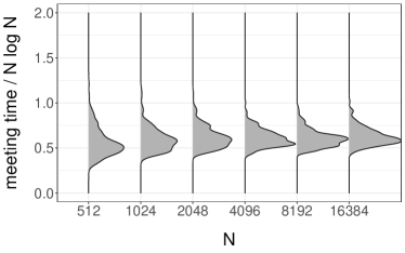
(a) Meeting times $/N\log N$

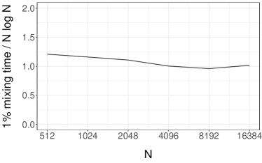
(b) Estimated $1\%$-mixing times $/N\log N$

Figure 1: Meeting times (left) and estimated upper bounds on the mixing time of the chain $x^{(t)}$ targeting $\text{CB}(p,I)$ (right), divided by $N\log N$, against $N$. Here the probabilities $p$ are independent Uniform(0,1) and $I=N/2$.

Our contribution is to refine the coupling argument in order to establish an upper bound on the mixing time of order $N\log N$, under conditions which allow for example $(p_{n})$ to be independent Uniform(0,1). A practical consequence of our result stated in Section 3.2 is that the simple MCMC algorithm is competitive compared to exact sampling strategies for $\text{CB}(p,I)$.

3 Proposed analysis

3.1 Favorable and unfavorable states

In the worst case scenario, $w_{a}$ might be of order $N^{-1}$ and $w_{b}$ of order $N$, resulting in a rate $c(x,\tilde{x})$ of order $N^{-2}$. However, this is not necessarily typical of a pair of states $(x,\tilde{x})\in\bar{\mathbb{X}}_{adj}$. This prompts us to partition $\bar{\mathbb{X}}_{adj}$ into “unfavorable” states, from which their probability of contracting is smaller than order $N^{-1}$, and “favorable” states, from which meeting occurs with probability of order $N^{-1}$. The precise definition of this partition will be made in relation to the odds $(w_{n})$. Since $c(x,\tilde{x})$ in (1) depends on $(w_{n})$ and $I$, we will care about statements holding with high probability under the distribution of $(w_{n})$ and $I$, which are described in Assumptions 3.1 and 3.2. Fortunately, we will see in Proposition 3.1 that favorable states can be reached from unfavorable ones with probability at least order $N^{-1}$, while unfavorable states are visited from favorable ones with probability less than order $N^{-1}$. This will prove enough for us to establish a mixing time of order $N\log N$ in Theorem 1.

Assumption 3.1.

(Condition on the odds). The odds $(w_{n})$ are such that there exist $\zeta>0$, $0<l<r<\infty$ and $\eta>0$ such that for all $N$ large enough,

$$\mathbb{P}\left(\left|\left\{n\in[N]:w_{n}\notin(l,r)\right\}\right|\leq\zeta N\right)\geq 1-\exp(-\eta N).$$

This assumption states that with exponentially high probability, a proportion of the odds that falls within an interval can be defined independently of $N$. The condition can be verified using for example Hoeffding’s inequality if the odds $(w_{n})$ are independently and identically distributed on $(0,\infty)$, but also under weaker conditions. The statement “for all $N$ large enough” means for all $N\geq N_{0}$ where $N_{0}\in\mathbb{N}$.

Assumption 3.2.

(Conditions on $I$). There exist $0<\xi\leq 1/2$ and $\eta^{\prime}>0$ such that for all $N$ large enough,

$$\mathbb{P}\left(\xi N\leq I\right)\geq 1-\exp(-\eta^{\prime}N).$$

This assumption formalizes what we mean by $I\propto N$, and is probabilistic rather than setting $I=\lfloor\xi N\rfloor$ for some $\xi\in(0,1/2]$. It implies that $\xi N^{2}/2\leq(N-I)I\leq(1-\xi)N^{2}/2$ with high probability. Recall that we have assumed $I\leq N/2$ without loss of generality.

Proposition 3.1.

Suppose Assumptions 3.1 and 3.2 hold such that $\zeta<\xi$. Then we can define $\xi_{\mathrm{F}\to\mathrm{D}},\xi_{\mathrm{U}\to\mathrm{F}},\xi_{\mathrm{F}\to\mathrm{U}},\nu>0$ and $0<w_{lo}<w_{hi}<\infty$ such that, for all $N$ large enough, with probability at least $1-\exp(-\nu N)$, the sets of favorable and unfavorable states defined as

$$\bar{\mathbb{X}}_{\mathrm{U}} =\{(x,\tilde{x})\in\bar{\mathbb{X}}_{adj}:w_{a}<w_{lo}\text{ and }w_{b}>w_{hi}\},$$ (2)

$$\bar{\mathbb{X}}_{\mathrm{F}} =\{(x,\tilde{x})\in\bar{\mathbb{X}}_{adj}:w_{a}\geq w_{lo}\ \text{ or }\ w_{b}\leq w_{hi}\},$$ (3)

and the “diagonal” set $\bar{\mathbb{X}}_{\mathrm{D}}=\{(x,\tilde{x})\in\mathbb{X}^{2}:x=\tilde{x}\}$, satisfy the following statements under the coupling $\bar{P}$ described in Section 2.2,

$$\bar{P}((x,\tilde{x}),\bar{\mathbb{X}}_{\mathrm{D}}) \geq\xi_{\mathrm{F}\to\mathrm{D}}/N,\quad\forall(x,\tilde{x})\in\bar{\mathbb{X}}_{\mathrm{F}},$$ (4)

$$\bar{P}((x,\tilde{x}),\bar{\mathbb{X}}_{\mathrm{F}}) \geq\xi_{\mathrm{U}\to\mathrm{F}}/N,\quad\forall(x,\tilde{x})\in\bar{\mathbb{X}}_{\mathrm{U}},$$ (5)

$$\bar{P}((x,\tilde{x}),\bar{\mathbb{X}}_{\mathrm{U}}) \leq\xi_{\mathrm{F}\to\mathrm{U}}/N,\quad\forall(x,\tilde{x})\in\bar{\mathbb{X}}_{\mathrm{F}}.$$ (6)

The proof in Appendix D.1 relies on a careful inspection of the various cases arising in the propagation of the coupled chains. The proposition provides bounds on the transition probabilities between the subsets $\bar{\mathbb{X}}_{\mathrm{U}}$, $\bar{\mathbb{X}}_{\mathrm{F}}$ and $\bar{\mathbb{X}}_{\mathrm{D}}$.

3.2 Chasing chain and mixing time

We relate the coupled chain $(x^{(t)},\tilde{x}^{(t)})$ to an auxiliary Markov chain denoted by $(Z^{(t)})$, defined on a space with three states $\{1,2,3\}$, associated with the subsets $\bar{\mathbb{X}}_{\mathrm{U}}$, $\bar{\mathbb{X}}_{\mathrm{F}}$ and $\bar{\mathbb{X}}_{\mathrm{D}}$, respectively. We introduce the Markov transition matrix

$$Q=\begin{pmatrix}1-\xi_{\mathrm{U}\to\mathrm{F}}/N&\xi_{\mathrm{U}\to\mathrm{F}}/N&0\\ \xi_{\mathrm{F}\to\mathrm{U}}/N&1-\xi_{\mathrm{F}\to\mathrm{U}}/N-\xi_{\mathrm{F}\to\mathrm{D}}/N&\xi_{\mathrm{F}\to\mathrm{D}}/N\\ 0&0&1\end{pmatrix},$$ (7)

where the constants $\xi_{\mathrm{F}\to\mathrm{D}},\xi_{\mathrm{U}\to\mathrm{F}},\xi_{\mathrm{F}\to\mathrm{U}}>0$ are given by Proposition 3.1, and we assume $N$ is large enough for each entry, including $1-\xi_{\mathrm{U}\to\mathrm{F}}/N$ and $1-\xi_{\mathrm{F}\to\mathrm{U}}/N-\xi_{\mathrm{F}\to\mathrm{D}}/N$, to be positive. We then observe that a Markov chain $(Z^{(t)})$ with transition $Q$ is such that there exists $r\in(0,1)$ independent of $N$ satisfying $\mathbb{P}(Z^{(N)}=3|Z^{(0)}=1)\geq 1-r$; details can be found in Appendix D.2.

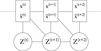
Figure 2: Conditional dependencies of the processes $(x^{(t)},\tilde{x}^{(t)})$ and $(Z^{(t)})$.

We now relate the auxiliary chain to $(x^{(t)},\tilde{x}^{(t)})$ using a strategy inspired by Jacob and Ryder (2014). Consider the variable $B^{(t)}\in\{1,2,3\}$ defined as $1$ if $(x^{(t)},\tilde{x}^{(t)})\in\bar{\mathbb{X}}_{\mathrm{U}}$, $2$ if $(x^{(t)},\tilde{x}^{(t)})\in\bar{\mathbb{X}}_{\mathrm{F}}$ and $3$ if $x^{(t)}=\tilde{x}^{(t)}$. The key idea is to construct the auxiliary chain $(Z^{(t)})$ on $\{1,2,3\}$, in such a way that it is (marginally) a Markov chain with transition matrix $Q$ in (7), and also such that $Z^{(t)}\leq B^{(t)}$ for all $t$ almost surely; this is possible thanks to Proposition 3.1. Thus the event $\{Z^{(t)}=3\}$ will imply $\{B^{(t)}=3\}=\{x^{(t)}=\tilde{x}^{(t)}\}$, and we can translate the hitting time of $(Z^{(t)})$ to its absorbing state into a statement about the meeting time of $(x^{(t)},\tilde{x}^{(t)})$. An explicit construction of $(Z^{(t)})$ is described in Appendix D.3; Figure 2 represents the dependency structure where $Z^{(t+1)}$ is constructed given $Z^{(t)}$, but also conditional upon $(x^{(t)},\tilde{x}^{(t)})$ and $(x^{(t+1)},\tilde{x}^{(t+1)})$ to ensure that the inequality $Z^{(t+1)}\leq B^{(t+1)}$ holds almost surely.

The convergence of $(Z^{(t)})$ to its absorbing state translates into an upper bound on the mixing time of $(x^{(t)})$ of the order of $N\log N$ iterations, which is our main result.

Theorem 1.

Under Assumptions 3.1 and 3.2 such that $\zeta<\xi$, there exist $\kappa>0$, $\nu>0$, $N_{0}\in\mathbb{N}$ independent of $N$ such that, for any $\epsilon\in(0,1)$, and for all $N\geq N_{0}$, with probability at least $1-\exp(-\nu N)$, we have

$$\|x^{(t)}-\text{CB}(p,I)\|_{\mathrm{TV}}\leq\epsilon\quad\text{ for all }\quad t\geq\kappa N\log(N/\epsilon).$$

The proof of Theorem 1 is given in Appendix D.4.

4 Discussion

Using the strategy of Biswas et al. (2019), we assess the convergence rate of the chain in the regime where $I$ is sub-linear in $N$. Figure 3 shows the estimated upper bounds on the mixing time obtained in the case where $I$ is fixed to $10$ while $N$ grows, and where $(p_{n})$ are independent Uniform(0,1) (generated once for each value of $N$). The figure might suggest that the mixing time grows at a slower rate than $N$ in this setting, and thus that MCMC is competitive relative to exact sampling. Understanding the small $I$ regime remains an open problem.

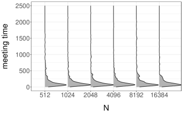
(a) Meeting times

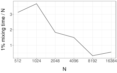
(b) Estimated $1\%$-mixing times divided by $N$

Figure 3: Meeting times (left) and estimated upper bounds on the mixing time, divided by $N$ (right), against $N$. The probabilities $p$ are independent Uniform(0,1) and $I=10$ for all $N$.

Our approach relies on a partition of the state space and an auxiliary Markov chain defined on the subsets given by the partition. This technique bear a resemblance to partitioning the state space with more common drift and contraction conditions (Durmus and Moulines, 2015; Qin and Hobert, 2019), but appears to be distinct.

The present setting is similar to the question of sampling permutations via random swaps. For that problem, direct applications of the coupling argument result in upper bounds on the mixing time of the order of at least $N^{2}$. Bormashenko (2011) devises an original variant of the path coupling strategy to obtain an upper bound in $N\log N$, which is the correct dependency on $N$; see Berestycki and Şengül (2019) for recent developments leading to sharp constants.

The proposed analysis captures the impact of the dimension $N$ faithfully. It fails to provide accurate constants and exact characterizations of how the mixing time depends on the distribution of the probabilities $(p_{n})$ and the sum $I$. Yet our analysis already supports the use of MCMC over exact sampling strategies for conditional Bernoulli sampling, especially as part of encompassing MCMC algorithms such as that of Yang et al. (2016) for Bayesian variable selection.

Acknowledgments

This work was funded by CY Initiative of Excellence (grant “Investissements d’Avenir” ANR-16-IDEX-0008). Pierre E. Jacob gratefully acknowledges support by the National Science Foundation through grants DMS-1712872 and DMS-1844695.

Appendix A Exact sampling of conditional Bernoulli

We describe a procedure to sample exactly from $\text{CB}(p,I)$ for a cost of order $N^{2}$. First, compute a $(I+1)\times N$ matrix of entries $q(i,n)$, for $i\in\{0,\ldots,I\},n\in[N]$, where $q(i,n)=\mathbb{P}(\sum_{m=n}^{N}x_{m}=i)$ with each $x_{n}$ independent Bernoulli$(p_{n})$. To compute these entries, proceed as follows. The initial conditions are given by

$$q(0,n)=\mathbb{P}\left(\sum_{m=n}^{N}x_{m}=0\right)=\prod_{m=n}^{N}\mathbb{P}(x_{m}=0)=\prod_{m=n}^{N}(1-p_{m}),\quad n\in[N],$$ (8)

in the case of no success, $q(1,N)=\mathbb{P}(x_{N}=1)=p_{N}$ where the sum reduces to a single Bernoulli variable, and $q(i,n)=0$ for $i>N-n+1$ because a sum of $N-n+1$ Bernoulli variables cannot be larger than $N-n+1$, in particular $q(i,N)=0$ for all $i\geq 2$. The other entries $q(i,n)$ can be obtained recursively, via

$$q(i,n)=p_{n}q(i-1,n+1)+(1-p_{n})q(i,n+1),\quad i\in[N],n\in[N-1].$$

Indeed, for $i\in[N]$ and $n\in[N-1]$, by conditioning on the value of $x_{n}\in\{0,1\}$, the law of total probability gives

$$q(i,n) =\mathbb{P}(x_{n}=1)\leavevmode\nobreak\ \mathbb{P}\left(\sum_{m=n}^{N}x_{m}=i\mid x_{n}=1\right)\leavevmode\nobreak\ +\leavevmode\nobreak\ \mathbb{P}(x_{n}=0)\leavevmode\nobreak\ \mathbb{P}\left(\sum_{m=n}^{N}x_{m}=i\mid x_{n}=0\right)$$

$$=p_{n}\leavevmode\nobreak\ \mathbb{P}\left(\sum_{m=n+1}^{N}x_{m}=i-1\right)\leavevmode\nobreak\ +\leavevmode\nobreak\ (1-p_{n})\leavevmode\nobreak\ \mathbb{P}\left(\sum_{m=n+1}^{N}x_{m}=i\right).$$ (9)

Having obtained the $(I+1)\times N$ entries $q(i,n)$, we now derive a sequential decomposition of a conditioned Bernoulli distribution that enables sampling in the order of $N$ operations. To sample $x_{1}$, we compute $\mathbb{P}(x_{1}=1|\sum_{n=1}^{N}x_{n}=i)$, as

$$\mathbb{P}\left(x_{1}=1|\sum_{n=1}^{N}x_{n}=i\right) =\frac{\mathbb{P}\left(x_{1}=1\right)\mathbb{P}\left(\sum_{n=1}^{N}x_{n}=i|x_{1}=1\right)}{\mathbb{P}\left(\sum_{n=1}^{N}x_{n}=i\right)}.$$ (10)

Note that the denominator is $q(i,1)$ and the numerator is $p_{1}q(i-1,2)$. Similarly for $n\in\{2,\ldots,N-1\}$,

$$\mathbb{P}\left(x_{n}=1|x_{1},\ldots,x_{n-1},\sum_{n=1}^{N}x_{n}=i\right) =\frac{\mathbb{P}\left(x_{n}=1\right)\mathbb{P}\left(\sum_{m=n}^{N}x_{m}=i-i_{n-1}|x_{n}=1\right)}{\mathbb{P}\left(\sum_{m=n}^{N}x_{m}=i-i_{n-1}\right)},$$ (11)

with $i_{n}=\sum_{m=1}^{n}x_{m}$. The numerator can be recognized as $p_{n}q(i-i_{n-1}-1,n+1)$ and the denominator as $q(i-i_{n-1},n)$. Lastly, given $x_{1},\ldots,x_{N-1},\sum_{n=1}^{N}x_{n}=i$, we can set $x_{N}$ to zero or one deterministically, namely $x_{N}=i-i_{N-1}$.

Appendix B Contractive coupling

B.1 Path coupling

Given current states $(x,\tilde{x})\in\mathbb{X}^{2}$, let $(x^{\prime},\tilde{x}^{\prime})\sim\bar{P}((x,\tilde{x}),\cdot)$ denote new states sampled from $\bar{P}((x,\tilde{x}),\cdot)$, a coupling of $P(x,\cdot)$ and $P(\tilde{x},\cdot)$. We want to establish the contraction

$$\mathbb{E}\left[d(x^{\prime},\tilde{x}^{\prime})|x,\tilde{x}\right]\leq(1-c)d(x,\tilde{x}),\quad\forall(x,\tilde{x})\in\mathbb{X}^{2},$$ (12)

with a large contraction rate $c\in(0,1)$. The path coupling argument [Bubley and Dyer, 1997, Guruswami, 2000] allows us to reduce the task in (12) to contraction from pairs of adjacent states, i.e.

$$\mathbb{E}\left[d(x^{\prime},\tilde{x}^{\prime})|x,\tilde{x}\right]\leq(1-c)d(x,\tilde{x}),\quad\forall(x,\tilde{x})\in\bar{\mathbb{X}}_{adj}.$$ (13)

It operates as follows. Suppose that (13) holds under the coupling $\bar{P}$. For two arbitrary states $(x,\tilde{x})\notin\bar{\mathbb{X}}_{adj}$ with $d(x,\tilde{x})=D>2$, we consider a “path” $x=z_{0},z_{1},\ldots,z_{L}=\tilde{x}$ of $L=D/2$ adjacent elements (i.e. $d(z_{\ell},z_{\ell+1})=2$ for $\ell=0,\ldots,L-1$). By construction the sum $\sum_{\ell=1}^{L}d(z_{\ell-1},z_{\ell})$ equals $D$. As there could be multiple such paths, to remove any ambiguity, we define a deterministic path by going through $x$ and $\tilde{x}$ from left to right, introducing a new element in the path for each encountered discrepancy. We then generate the new states $(x^{\prime},\tilde{x}^{\prime})$ using the following procedure:

1. sample $(z_{0}^{\prime},z_{1}^{\prime})\sim\bar{P}((z_{0},z_{1}),\cdot)$,

2. for $\ell=2,\ldots,L$, sample $z^{\prime}_{\ell}$ from the conditional of $\bar{P}((z_{\ell-1},z_{\ell}),(z^{\prime}_{\ell-1},z_{\ell}^{\prime}))$ given $z^{\prime}_{\ell-1}$,

3. set $x^{\prime}=z^{\prime}_{0}$ and $\tilde{x}^{\prime}=z^{\prime}_{L}$.

By construction we have $\tilde{x}^{\prime}|\tilde{x}\sim P(\tilde{x},\cdot)$, thus this scheme defines a coupling of $P(x,\cdot)$ and $P(\tilde{x},\cdot)$. Under the above coupling, we have

$$\mathbb{E}\left[d(x^{\prime},\tilde{x}^{\prime})|x,\tilde{x}\right] =\mathbb{E}\left[d(x^{\prime},\tilde{x}^{\prime})|x=z_{0},\ldots,z_{L}=\tilde{x}\right]$$

$$\leq\mathbb{E}\left[\sum_{\ell=1}^{L}d(z^{\prime}_{\ell-1},z^{\prime}_{\ell})|x=z_{0},\ldots,z_{L}=\tilde{x}\right] =\sum_{\ell=1}^{L}\mathbb{E}\left[d(z^{\prime}_{\ell-1},z^{\prime}_{\ell})|z{}_{\ell-1},z{}_{\ell}\right]\leq\sum_{\ell=1}^{L}(1-c)d(z_{\ell-1},z_{\ell}),$$

for any $(x,\tilde{x})\notin\bar{\mathbb{X}}_{adj}$. The first equality holds because $(z_{\ell})$ is obtained deterministically given $x,\tilde{x}$. The rest follow from triangle inequalities, linearity of expectation, conditional independencies between the variables introduced in the coupling construction, and the assumption of contraction from adjacent states in (13). The last expression is equal to $(1-c)d(x,\tilde{x})$ by construction of the path. In summary, the path coupling argument allows us to extend contraction between adjacent states (13) to contraction for any pair of states (12) with the same rate.

B.2 Contraction rate of $\bar{P}$ for adjacent states

We compute the contraction rate $c(x,\tilde{x})$ in (1) under $\bar{P}$, the coupling described in Section 2.2.

The coupling of $(i_{0},\tilde{i}_{0})$ is such that $\mathbb{P}(i_{0}=a,\tilde{i}_{0}=b)=(N-I)^{-1}$. Similarly the maximal coupling on $(i_{1},\tilde{i}_{1})$ leads to $\mathbb{P}(i_{1}=b,\tilde{i}_{1}=a)=I^{-1}$. Under that coupling, if none of the indices $i_{0},\tilde{i}_{0},i_{1},\tilde{i}_{1}$ are in $\{a,b\}$, then the proposed swaps will be either accepted or rejected jointly and the distance $d(x,\tilde{x})$ will be unchanged. We consider proposed swaps that could affect the discrepancy.

1. The index $i_{0}$ can be equal to $a$ (with probability $(N-I)^{-1}$). In that case, $\tilde{i}_{0}$ must be equal to $b$, which is the only index in $\tilde{S}_{0}$ that is not in $S_{0}$; this comes from the maximal coupling strategy for sampling $(i_{0},\tilde{i}_{0})$. The index $i_{1}$ can be equal to $b$ (with probability $I^{-1}$), in which case $\tilde{i}_{1}=a$ again due to the maximal coupling strategy. The discrepancy is then reduced if exactly one of the two proposed swaps is accepted, which happens with probability

   $$\left|\min\left(1,\frac{w_{i_{0}}}{w_{i_{1}}}\right)-\min\left(1,\frac{w_{\tilde{i}_{0}}}{w_{\tilde{i}_{1}}}\right)\right|=|1-w_{a}/w_{b}|.$$

2. The index $i_{0}$ can be equal to $a$ (again with probability $(N-I)^{-1}$) and $i_{1}$ not equal to $b$ (with probability $(I-1)I^{-1}$). Then $\tilde{i}_{1}=i_{1}$ (maximum coupling), and given $i_{1}\neq b$, the discrepancy is reduced if both proposed swaps are accepted. The probability of reducing the discrepancy given $\{i_{0}=a,i_{1}\neq b$} is

   $$\frac{1}{I-1}\sum_{i_{1}\in S_{1}\cap\tilde{S}_{1}}\min\left(1,\frac{w_{a}}{w_{i_{1}}}\right).$$

3. The index $i_{0}$ can be different from $a$, in which case $\tilde{i}_{0}=i_{0}$, and the discrepancy might be reduced if $i_{1}=b$, $\tilde{i}_{1}=a$ and both swaps are accepted. Given $\{i_{0}\neq a,\tilde{i}_{1}=b\}$ this occurs with probability

   $$\frac{1}{N-I-1}\sum_{i_{0}\in S_{0}\cap\tilde{S}_{0}}\min\left(1,\frac{w_{i_{0}}}{w_{b}}\right).$$

The contraction rate in (1) follows from summing up the above three possibilities.

Appendix C Estimation of upper bounds on the mixing time

We briefly describe the choices made in applying the $L$-lag coupling approach of Biswas et al. [2019].

For the choice of coupling, we implemented the kernel $\bar{P}$ presented in Section 2.2. A careful implementation of the kernel, by keeping track of the four sets $S_{ij}$ of indices $n$ such that $x_{n}=i,\tilde{x}_{n}=j$ for $i,j\in\{0,1\}$, results in a constant cost per iteration of the coupled chain. The chains are initialized by sampling $I$ indices without replacement in binary vectors of length $N$, and setting these components to one and the others to zero.

We use a lag of $L=1$, and run $500$ independent runs of coupled lagged chains, to obtain as many realizations of the meeting time $\tau$. We employ the key identity in Biswas et al. [2019],

$$\|x^{(t)}-\text{CB}(p,I)\|_{\text{TV}}\leq\mathbb{E}\left[\max\left(0,\left\lceil\frac{\tau-L-t}{L}\right\rceil\right)\right].$$

The expectation on the right hand side is estimated by an average of independent copies of the meeting time, for any desired iteration $t$. As the estimate is itself decreasing in $t$, we can find the smallest $t$ such that the estimate is less than $\epsilon=0.01$, and this provides an estimated upper bound on the $\epsilon$-mixing time.

Appendix D Proofs

D.1 Proof of Proposition 3.1

Under the assumptions, we define $0<w_{lo}<w_{hi}<\infty$ and $\delta>0$ such that $w_{lo}+\delta=l$ and $w_{hi}-\delta=r$, with $(l,r)$ as the interval in Assumption 3.1. The assumption thus guarantees that with high probability, the number of odds in $(w_{n})$ that are outside of $(w_{lo}+\delta,w_{hi}-\delta)$ is less than $\zeta N$. In particular, the number of odds above $w_{hi}$, and the number of odds below $w_{lo}$ are both less than $\zeta N$. The $\delta$ term can be arbitrarily small and is helpful in a calculation below.

Proof of (4). We start with the transition from $\bar{\mathbb{X}}_{\mathrm{F}}$ to $\bar{\mathbb{X}}_{\mathrm{D}}$. Assume $(x,\tilde{x})\in\bar{\mathbb{X}}_{\mathrm{F}}$. For such states, $w_{a}>w_{lo}$ or $w_{b}<w_{hi}$, therefore the contraction rate $c(x,\tilde{x})$ (1) is at least

$$\frac{1}{I(N-I)}\left\{\sum_{i_{1}\in S_{1}\cap\tilde{S}_{1}}\min(1,w_{lo}/w_{i_{1}})\right\}\quad\text{ if $w_{a}>w_{lo}$,}$$

$$\frac{1}{I(N-I)}\left\{\sum_{i_{0}\in S_{0}\cap\tilde{S}_{0}}\min(1,w_{i_{0}}/w_{hi})\right\}\quad\text{ if $w_{b}<w_{hi}$}.$$

• First case ($w_{a}>w_{lo}$): Note that there are $I-1$ indices in $S_{1}\cap\tilde{S}_{1}$. Using Assumption 3.2, $I$ is at least $\xi N$ with high probability. Using Assumption 3.1, the number of odds in $(w_{n})$ above $w_{hi}$ is less than $\zeta N$. On the intersection of events, which is not empty if $N$ is large enough, among the $I-1$ entries in $S_{1}\cap\tilde{S}_{1}$, there are at least $(\xi-\zeta)N-1$ odds that are smaller than $w_{hi}$. The sum $\sum_{i_{1}\in S_{1}\cap\tilde{S}_{1}}\min(1,w_{lo}/w_{i_{1}})$ is thus larger than $((\xi-\zeta)N-1)w_{lo}/w_{hi}$. We obtain the lower bound

  $$\bar{P}((x,\tilde{x}),\bar{\mathbb{X}}_{\mathrm{D}})\geq 2(1-\xi)^{-1}N^{-2}\cdot((\xi-\zeta)N-1)w_{lo}/w_{hi}.$$

• Second case ($w_{b}<w_{hi}$): In that case, among the $N-I-1$ indices in $S_{0}\cap\tilde{S}_{0}$, under the assumptions there are at least $(1/2-\zeta)N-1$ components of $(w_{n})$ that are larger than $w_{lo}$. Thus the sum $\sum_{i_{0}\in S_{0}\cap\tilde{S}_{0}}\min(1,w_{i_{0}}/w_{hi})$ is larger than $((1/2-\zeta)N-1)w_{lo}/w_{hi}$, and we obtain the lower bound

  $$\bar{P}((x,\tilde{x}),\bar{\mathbb{X}}_{\mathrm{D}})\geq 2(1-\xi)^{-1}N^{-2}\cdot((1/2-\zeta)N-1)w_{lo}/w_{hi}.$$

From the two cases, we obtain for $N$ large enough a lower bound of the form $\xi_{\mathrm{F}\to\mathrm{D}}/N$ for some $\xi_{\mathrm{F}\to\mathrm{D}}>0$.

Proof of (5). We next consider the probability of transitioning from $\bar{\mathbb{X}}_{\mathrm{U}}$ to $\bar{\mathbb{X}}_{\mathrm{F}}$. For any $(x,\tilde{x})\in\bar{\mathbb{X}}_{\mathrm{U}}$, such transitions occurs in two distinct cases.

• We propose swapping component $i_{0}=a$ and $i_{1}\neq b$, and $\tilde{i}_{0}=b$ and $\tilde{i}_{1}=i_{1}$, such that $w_{i_{1}}<w_{hi}$, and exactly one of the two swaps is accepted. In that case $b$ becomes $i_{1}$.

• We propose swapping component $i_{1}=b$ and $i_{0}\neq a$, and $\tilde{i}_{0}=i_{0}$ and $\tilde{i}_{1}=a$, such that $w_{i_{0}}>w_{lo}$, and exactly one of the two swaps is accepted. In that case $a$ becomes $i_{0}$.

Note that the case of swapping components $a$ and $b$ results in an unfavorable state, upon relabeling of the states $x$ and $\tilde{x}$ to maintain $w_{a}\leq w_{b}$. As we only seek a lower bound of $\xi_{\mathrm{U}\to\mathrm{F}}/N$ in (5), it is sufficient to only consider the first case. Since $w_{a}\leq w_{b}$, if only one swap is accepted, it must be the one on the $\tilde{x}$ chain; then $b$ becomes $i_{1}$ and $a$ remains unchanged.

Selection of $i_{0}=a$ and $i_{1}\neq b$ occurs with probability $(N-I)^{-1}\times(I-1)I^{-1}$. Acceptance of exactly one swap occurs with probability $|\min(1,w_{a}/w_{i_{1}})-\min(1,w_{b}/w_{i_{1}})|$. Thus the probability of moving to $\bar{\mathbb{X}}_{\mathrm{F}}$ via the acceptance of one swap is at least

$$\frac{1}{(N-I)I}\sum_{i_{1}\in S_{1}\setminus\{b\}}|\min(1,w_{a}/w_{i_{1}})-\min(1,w_{b}/w_{i_{1}})|\mathds{1}(w_{i_{1}}<w_{hi})$$

$$=\frac{1}{(N-I)I}\sum_{i_{1}\in S_{1}\setminus\{b\}}|1-\min(1,w_{a}/w_{i_{1}})|\mathds{1}(w_{i_{1}}<w_{hi})\quad\text{because $w_{b}>w_{hi}$}$$

$$\geq\frac{1}{(N-I)I}\sum_{i_{1}\in S_{1}\setminus\{b\}}|1-\min(1,w_{a}/w_{i_{1}})|\mathds{1}(w_{lo}+\delta<w_{i_{1}}<w_{hi})\quad\text{because fewer terms}$$

$$\geq\frac{1}{(N-I)I}\sum_{i_{1}\in S_{1}\setminus\{b\}}|1-w_{a}/(w_{lo}+\delta)|\mathds{1}(w_{lo}+\delta<w_{i_{1}}<w_{hi})$$

$$\geq\frac{1}{(N-I)I}((\xi-\zeta)N-1)|1-w_{a}/(w_{lo}+\delta)|.$$

The last inequality holds when $I\geq\xi N$, and when at most $\zeta N$ entries of $(w_{n})$ are outside of $(w_{lo}+\delta,w_{hi})$; again we work in the intersection of the high probability events specified by the assumptions.

We conclude by noting that, for $w_{a}<w_{lo}$, we have $|1-w_{a}/(w_{lo}+\delta)|\geq\delta/(w_{lo}+\delta)$, which is a constant independent of $N$; this is where the $\delta$ term comes in handy. Thus for $(x,\tilde{x})\in\bar{\mathbb{X}}_{\mathrm{U}}$, we can move to $\bar{\mathbb{X}}_{\mathrm{F}}$ with probability

$$\bar{P}((x,\tilde{x}),\bar{\mathbb{X}}_{\mathrm{F}})\geq 2(1-\xi)^{-1}N^{-2}\cdot((\xi-\zeta)N-1)\delta/(w_{lo}+\delta),$$

which is at least $\xi_{\mathrm{U}\to\mathrm{F}}/N$ for some $\xi_{\mathrm{U}\to\mathrm{F}}>0$ as $N$ gets large.

Proof of (6). We finally consider the probability of moving from $\bar{\mathbb{X}}_{\mathrm{F}}$ to $\bar{\mathbb{X}}_{\mathrm{U}}$. As we want an upper bound of this quantity, we have to consider all possible routes from $(x,\tilde{x})\in\bar{\mathbb{X}}_{\mathrm{F}}$ to $\bar{\mathbb{X}}_{\mathrm{U}}$. If the state is such that $w_{a}>w_{lo}$ and $w_{b}<w_{hi}$, then the pair cannot transition to an unfavorable state. In other words, $\bar{P}((x,\tilde{x}),\bar{\mathbb{X}}_{\mathrm{U}})$ can be equal to zero. Transition to an unfavorable state occurs in two distinct cases:

• if $w_{a}<w_{lo}$, $w_{b}<w_{hi}$, and if the swap changes $b$ to some $i_{1}$ with $w_{i_{1}}>w_{hi}$;

• if $w_{b}>w_{hi}$, $w_{a}>w_{lo}$, and if the swap changes $a$ to some $i_{0}$ with $w_{i_{0}}<w_{lo}$.

The first case happens if the drawn indices are $(i_{0},\tilde{i}_{0})=(a,b)$ and $i_{1}=\tilde{i}_{1}$ in $S_{1}\setminus\{b\}$ such that $w_{i_{1}}>w_{hi}$, and if we accept the swap for the chain $\tilde{x}$ but not for $x$, which occurs with probability $(w_{b}-w_{a})/w_{i_{1}}$. Thus the probability associated with this transition is

$$\frac{1}{(N-I)I}\left\{\sum_{i_{1}\in S_{1}:w_{i_{1}}>w_{hi}}(w_{b}-w_{a})/w_{i_{1}}\right\}\leq\frac{1}{(N-I)I}\sum_{i_{1}\in S_{1}}\mathds{1}(w_{i_{1}}>w_{hi})\leq 2\xi^{-1}N^{-2}\cdot\zeta N,$$

in the event that the number of odds above $w_{hi}$ is less than $\zeta N$.

The second case occurs if the drawn indices are $i_{0}=\tilde{i}_{0}$ in $S_{0}\setminus\{a\}$ with $w_{i_{0}}<w_{lo}$ and $(i_{1},\tilde{i}_{1})=(b,a)$, and if we accept the swap for the chain $\tilde{x}$ but not for $x$, which occurs with probability $w_{i_{0}}\cdot(w_{a}^{-1}-w_{b}^{-1})\leq 1$. The probability associated with this transition is at most

$$\frac{1}{(N-I)I}\left\{\sum_{i_{0}\in S_{0}:w_{i_{0}}<w_{lo}}w_{i_{0}}\cdot(w_{a}^{-1}-w_{b}^{-1})\right\}\leq\frac{1}{(N-I)I}\sum_{i_{0}\in S_{0}}\mathds{1}(w_{i_{0}}<w_{lo})\leq 2\xi^{-1}N^{-2}\cdot\zeta N,$$

in the event that fewer than $\zeta N$ odds are below $w_{lo}$. Thus for $(x,\tilde{x})\in\bar{\mathbb{X}}_{\mathrm{F}}$, we can upper bound $\bar{P}((x,\tilde{x}),\bar{\mathbb{X}}_{\mathrm{U}})$ by $\xi_{\mathrm{F}\to\mathrm{U}}/N$ for some $\xi_{\mathrm{F}\to\mathrm{U}}>0$.

D.2 Convergence of the Markov chain with transition $Q$

The second largest left-eigenvalue of $Q$ in (7) is

$$1-\frac{1}{2N}\left(\xi_{\mathrm{F}\to\mathrm{D}}+\xi_{\mathrm{F}\to\mathrm{U}}+\xi_{\mathrm{U}\to\mathrm{F}}-\sqrt{\left(\xi_{\mathrm{F}\to\mathrm{D}}+\xi_{\mathrm{F}\to\mathrm{U}}+\xi_{\mathrm{U}\to\mathrm{F}}\right)^{2}-4\xi_{\mathrm{F}\to\mathrm{D}}\xi_{\mathrm{U}\to\mathrm{F}}}\right).$$

This is of order $1-\alpha/N$ for a positive constant $\alpha$, for all $\xi_{\mathrm{F}\to\mathrm{D}},\xi_{\mathrm{U}\to\mathrm{F}},\xi_{\mathrm{F}\to\mathrm{U}}>0$. Using the fact that $(1-\alpha/N)^{N}$ is less than $\exp(-\alpha)$ for all $\alpha>0$, we can lower bound the probability $\mathbb{P}(Z^{(N)}=3|Z^{(0)}=1)$ by a constant independent of $N$.

D.3 Construction of the auxiliary chain

We now detail the construction of the auxiliary chain $(Z^{(t)})$. The construction is done conditionally on $(x^{(t)},\tilde{x}^{(t)})$. We refer readers to Figure 2 and recall that $B^{(t)}$ is a deterministic function of $(x^{(t)},\tilde{x}^{(t)})$. Note that the dependencies shown in Figure 2 are a consequence of the following construction.

First, if $Z^{(t)}=1$, we construct $Z^{(t+1)}$ as follows.

• If $B^{(t)}=1$ or $B^{(t)}=2$,

  • if $B^{(t+1)}=1$ set $Z^{(t+1)}=1$,

  • otherwise, set $Z^{(t+1)}=2$ with probability $(\xi_{\mathrm{U}\to\mathrm{F}}/N)/\mathbb{P}(B^{(t+1)}\in\{2,3\}|x^{(t)},\tilde{x}^{(t)})$, and set $Z^{(t+1)}=1$ otherwise.

• If $B^{(t)}=3$, sample $Z^{(t+1)}$ from $\{1,2,3\}$ using the probabilities in the first row of (7).

Let us check that the above transition probabilities are well-defined and lie in $[0,1]$. If $B^{(t)}=1$, $(\xi_{\mathrm{U}\to\mathrm{F}}/N)/\mathbb{P}(B^{(t+1)}\in\{2,3\}|x^{(t)},\tilde{x}^{(t)})$ is less than $(\xi_{\mathrm{U}\to\mathrm{F}}/N)/\mathbb{P}(B^{(t+1)}=2|x^{(t)},\tilde{x}^{(t)})$ which is less than one by Proposition 3.1, Equation (5). If $B^{(t)}=2$, $(\xi_{\mathrm{U}\to\mathrm{F}}/N)/\mathbb{P}(B^{(t+1)}\in\{2,3\}|x^{(t)},\tilde{x}^{(t)})$ is less than one if $N$ is large enough, using Proposition 3.1 again. Indeed

$$\mathbb{P}(B^{(t+1)}\in\{2,3\}|x^{(t)},\tilde{x}^{(t)})=1-\mathbb{P}(B^{(t+1)}=1|x^{(t)},\tilde{x}^{(t)})\geq 1-\xi_{\mathrm{F}\to\mathrm{U}}/N,$$

by Equation (6), and this is larger than $\xi_{\mathrm{U}\to\mathrm{F}}/N$ if $N$ is large enough, for any $\xi_{\mathrm{U}\to\mathrm{F}},\xi_{\mathrm{F}\to\mathrm{U}}$.

The goal of this construction is that $Z^{(t+1)}=2$ only if $B^{(t+1)}\in\{2,3\}$, so that $Z^{(t+1)}\leq B^{(t+1)}$ holds almost surely. We can compute

$$\mathbb{P}(Z^{(t+1)}=2|Z^{(t)}=1,x^{(t)},\tilde{x}^{(t)}) =\mathbb{P}(Z^{(t+1)}=2,B^{(t+1)}=1|Z^{(t)}=1,x^{(t)},\tilde{x}^{(t)})$$

$$+\mathbb{P}(Z^{(t+1)}=2,B^{(t+1)}\in\{2,3\}|Z^{(t)}=1,x^{(t)},\tilde{x}^{(t)}),$$

which, using the conditional dependencies implied by the construction is equal to

$$0+ \mathbb{P}(Z^{(t+1)}=2|B^{(t+1)}\in\{2,3\},Z^{(t)}=1,x^{(t)},\tilde{x}^{(t)})\times\mathbb{P}(B^{(t+1)}\in\{2,3\}|x^{(t)},\tilde{x}^{(t)})=\xi_{\mathrm{U}\to\mathrm{F}}/N,$$

for all values of $B^{(t)}$ in $\{1,2,3\}$. Since the probability $\mathbb{P}(Z^{(t+1)}=2|Z^{(t)}=1,x^{(t)},\tilde{x}^{(t)})$ is the same for all $(x^{(t)},\tilde{x}^{(t)})$, we deduce that $\mathbb{P}(Z^{(t+1)}=2|Z^{(t)}=1)=\xi_{\mathrm{U}\to\mathrm{F}}/N$.

We proceed similarly for the second row of (7), assuming $Z^{(t)}=2$. In that case we must have $B^{(t)}\geq 2$. Consider the following construction.

• If $B^{(t)}=2$,

  • if $B^{(t+1)}=1$, set $Z^{(t+1)}=1$,

  • if $B^{(t+1)}=2$, sample $Z^{(t+1)}$ from $\{1,2,3\}$ with probabilities

    $$\left(\frac{\xi_{\mathrm{F}\to\mathrm{U}}/N-\mathbb{P}(B^{(t+1)}=1|x^{(t)},\tilde{x}^{(t)})}{\mathbb{P}(B^{(t+1)}=2|x^{(t)},\tilde{x}^{(t)})},1-\frac{\xi_{\mathrm{F}\to\mathrm{U}}/N-\mathbb{P}(B^{(t+1)}=1|x^{(t)},\tilde{x}^{(t)})}{\mathbb{P}(B^{(t+1)}=2|x^{(t)},\tilde{x}^{(t)})},0\right),$$

  • if $B^{(t+1)}=3$, sample $Z^{(t+1)}$ from $\{1,2,3\}$ with probabilities

    $$\left(0,1-\frac{\xi_{\mathrm{F}\to\mathrm{D}}/N}{\mathbb{P}(B^{(t+1)}=3|x^{(t)},\tilde{x}^{(t)})},\frac{\xi_{\mathrm{F}\to\mathrm{D}}/N}{\mathbb{P}(B^{(t+1)}=3|x^{(t)},\tilde{x}^{(t)})}\right).$$

• If $B^{(t)}=3$, sample $Z^{(t+1)}$ from $\{1,2,3\}$ using the probabilities in the second row of (7).

We can again verify that the probabilities are well-defined and lie in $[0,1]$, using Proposition 3.1 and assuming that $N$ is large enough so that $\mathbb{P}(B^{(t+1)}=2|x^{(t)},\tilde{x}^{(t)})+\mathbb{P}(B^{(t+1)}=1|x^{(t)},\tilde{x}^{(t)})\geq\xi_{\mathrm{F}\to\mathrm{U}}/N$.

Then we can compute

$$\mathbb{P}(Z^{(t+1)}=1|Z^{(t)}=2,x^{(t)},\tilde{x}^{(t)}) =\mathbb{P}(Z^{(t+1)}=1,B^{(t+1)}=1|Z^{(t)}=2,x^{(t)},\tilde{x}^{(t)})$$

$$+\mathbb{P}(Z^{(t+1)}=1,B^{(t+1)}=2|Z^{(t)}=2,x^{(t)},\tilde{x}^{(t)})+0.$$

If $B^{(t)}=2$, this becomes

$$1\times\mathbb{P}(B^{(t+1)}=1|x^{(t)},\tilde{x}^{(t)})$$

$$+ \left(\frac{\xi_{\mathrm{F}\to\mathrm{U}}/N-\mathbb{P}(B^{(t+1)}=1|x^{(t)},\tilde{x}^{(t)})}{\mathbb{P}(B^{(t+1)}=2|x^{(t)},\tilde{x}^{(t)})}\right)\times\mathbb{P}(B^{(t+1)}=2|x^{(t)},\tilde{x}^{(t)})$$

$$+ 0\times\mathbb{P}(B^{(t+1)}=3|x^{(t)},\tilde{x}^{(t)})=\xi_{\mathrm{F}\to\mathrm{U}}/N.$$

If $B^{(t)}=3$, we also have $\mathbb{P}(Z^{(t+1)}=1|Z^{(t)}=2,x^{(t)},\tilde{x}^{(t)})=\xi_{\mathrm{F}\to\mathrm{U}}/N$.

We next compute the transition from state $2$ to state $3$,

$$\mathbb{P}(Z^{(t+1)}=3|Z^{(t)}=2,x^{(t)},\tilde{x}^{(t)}) =\mathbb{P}(Z^{(t+1)}=3,B^{(t+1)}=1|Z^{(t)}=2,x^{(t)},\tilde{x}^{(t)})$$

$$\;+\;\mathbb{P}(Z^{(t+1)}=3,B^{(t+1)}=2|Z^{(t)}=2,x^{(t)},\tilde{x}^{(t)})$$

$$\;+\;\mathbb{P}(Z^{(t+1)}=3,B^{(t+1)}=3|Z^{(t)}=2,x^{(t)},\tilde{x}^{(t)}).$$

If $B^{(t)}=2$, this becomes

$$0\times\mathbb{P}(B^{(t+1)}=1|x^{(t)},\tilde{x}^{(t)})$$

$$\;+\;0\times\mathbb{P}(B^{(t+1)}=2|x^{(t)},\tilde{x}^{(t)})$$

$$\;+\;\frac{\xi_{\mathrm{F}\to\mathrm{D}}/N}{\mathbb{P}(B^{(t+1)}=3|x^{(t)},\tilde{x}^{(t)})}\times\mathbb{P}(B^{(t+1)}=3|x^{(t)},\tilde{x}^{(t)})=\xi_{\mathrm{F}\to\mathrm{D}}/N.$$

If $B^{(t)}=3$, we also find that $\mathbb{P}(Z^{(t+1)}=3|Z^{(t)}=2,x^{(t)},\tilde{x}^{(t)})=\xi_{\mathrm{F}\to\mathrm{D}}/N$. Again these probabilities do not depend on $B^{(t)}$ or $(x^{(t)},\tilde{x}^{(t)})$, thus the evolution of the chain $(Z^{(t)})$ given $Z^{(t)}=2$ is described by the second row of (7).

D.4 Upper bound on mixing time

Using the auxiliary chain $(Z^{(t)})$ we can state the following result about the $N$-th iteration of $\bar{P}$ from adjacent states.

Proposition D.1.

Under Assumptions 3.1 and 3.2 such that $\zeta<\xi$, we can define $r\in(0,1)$, $\nu>0$ and $N_{0}\in\mathbb{N}$ (independent of $N$) such that, for all $N\geq N_{0}$, with probability at least $1-\exp(-\nu N)$, under the coupled kernel $\bar{P}$

$$\mathbb{E}[d(x^{(N)},\tilde{x}^{(N)})|x^{(0)}=x,\tilde{x}^{(0)}=\tilde{x}]\leq r\,d(x,\tilde{x})=2r,$$

for any two states $(x,\tilde{x})\in\bar{\mathbb{X}}_{adj}$.

Proof of Proposition D.1.

Under the assumptions we can apply Proposition 3.1. We place ourselves on the large probability event from that proposition. This gives us the constants needed to define the transition matrix $Q$ in (7), the Markov chain $(Z^{(t)})$ with transition (7) and such that $Z^{(t)}\leq B^{(t)}$ for all $t\geq 0$ (almost surely), and the constant $r\in(0,1)$ such that $\mathbb{P}(Z^{(N)}=3|Z^{(0)}=1)\geq 1-r$. Based on the construction, $\mathbb{P}(x^{(N)}=\tilde{x}^{(N)})\geq\mathbb{P}(Z^{(N)}=3|Z^{(0)}=1)$, thus $\mathbb{P}(x^{(N)}=\tilde{x}^{(N)}|x^{(0)}=x,\tilde{x}^{(0)}=\tilde{x})\geq 1-r$. Noting that $\mathbb{E}[d(x^{(N)},\tilde{x}^{(N)})|x^{(0)}=x,\tilde{x}^{(0)}=\tilde{x}]=2\mathbb{P}(x^{(N)}\neq\tilde{x}^{(N)}|x^{(0)}=x,\tilde{x}^{(0)}=\tilde{x})$ concludes the proof. ∎

We can finally return to the path coupling argument, and apply it to a chain that follows $P^{N}$, the $N$-th iterate of the transition kernel of the original chain. From Proposition D.1, we have a contraction rate of $r\in(0,1)$ independently of $N$, for a coupling of $P^{N}$ from adjacent states, and we obtain the main theorem as follows.

Proof of Theorem 1.

The path coupling argument shows that for a chain $(\check{x}^{(t)})$ evolving according to $P^{N}$, there exist $\kappa,\nu>0$ such that for any $\epsilon>0$, with probability at least $1-\exp(-\nu N)$, we have

$$\|\check{x}^{(t)}-\text{CB}(p,I)\|_{\mathrm{TV}}\leq\epsilon\quad\text{ for all }\quad t\geq\kappa\log(N/\epsilon).$$

The variable $\check{x}^{(t)}$ has the same law as $x^{(tN)}$, thus with a change of time variable, $s=tN$, we obtain

$$\|{x}^{(s)}-\text{CB}(p,I)\|_{\mathrm{TV}}\leq\epsilon\quad\text{ for all }\quad s\geq\kappa N\log(N/\epsilon).$$

∎

References

- Berestycki and Şengül [2019] Nathanaël Berestycki and Batı Şengül. Cutoff for conjugacy-invariant random walks on the permutation group. Probability Theory and Related Fields, 173(3-4):1197–1241, 2019.
- Biswas et al. [2019] Niloy Biswas, Pierre E Jacob, and Paul Vanetti. Estimating convergence of Markov chains with L-lag couplings. In Advances in Neural Information Processing Systems, pages 7391–7401, 2019.
- Bormashenko [2011] Olena Bormashenko. A coupling argument for the random transposition walk. arXiv preprint arXiv:1109.3915, 2011.
- Broström and Nilsson [2000] Göran Broström and Leif Nilsson. Acceptance–rejection sampling from the conditional distribution of independent discrete random variables, given their sum. Statistics: A Journal of Theoretical and Applied Statistics, 34(3):247–257, 2000.
- Bubley and Dyer [1997] Russ Bubley and Martin Dyer. Path coupling: A technique for proving rapid mixing in Markov chains. In Proceedings 38th Annual Symposium on Foundations of Computer Science, pages 223–231. IEEE, 1997.
- Chen and Liu [1997] Sean X Chen and Jun S Liu. Statistical applications of the Poisson-Binomial and conditional Bernoulli distributions. Statistica Sinica, pages 875–892, 1997.
- Chen et al. [1994] Xiang-Hui Chen, Arthur P Dempster, and Jun S Liu. Weighted finite population sampling to maximize entropy. Biometrika, 81(3):457–469, 1994.
- Diaconis and Shahshahani [1987] Persi Diaconis and Mehrdad Shahshahani. Time to reach stationarity in the Bernoulli–Laplace diffusion model. SIAM Journal on Mathematical Analysis, 18(1):208–218, 1987.
- Donnelly et al. [1994] Peter Donnelly, Peter Lloyd, and Aidan Sudbury. Approach to stationarity of the Bernoulli–Laplace diffusion model. Advances in Applied Probability, 26(3):715–727, 1994.
- Durmus and Moulines [2015] Alain Durmus and Éric Moulines. Quantitative bounds of convergence for geometrically ergodic Markov chain in the Wasserstein distance with application to the Metropolis adjusted Langevin algorithm. Statistics and Computing, 25(1):5–19, 2015.
- Eskenazis and Nestoridi [2020] Alexandros Eskenazis and Evita Nestoridi. Cutoff for the Bernoulli–Laplace urn model with swaps. Ann. Inst. H. Poincaré Probab. Statist., 56(4):2621–2639, 11 2020. doi: 10.1214/20-AIHP1052. URL https://doi.org/10.1214/20-AIHP1052.
- Guruswami [2000] Venkatesan Guruswami. Rapidly mixing Markov chains: A comparison of techniques. Available: cs. washington. edu/homes/venkat/pubs/papers. html, 2000.
- Hough et al. [2006] J Ben Hough, Manjunath Krishnapur, Yuval Peres, and Bálint Virág. Determinantal processes and independence. Probability surveys, 3:206–229, 2006.
- Jacob and Ryder [2014] Pierre E Jacob and Robin J Ryder. The Wang–Landau algorithm reaches the flat histogram criterion in finite time. The Annals of Applied Probability, 24(1):34–53, 2014.
- Kulesza and Taskar [2012] Alex Kulesza and Ben Taskar. Determinantal point processes for machine learning. Foundations and Trends in Machine Learning, 5(2–3):123–286, 2012.
- Liu et al. [1995] Jun S Liu, Andrew F Neuwald, and Charles E Lawrence. Bayesian models for multiple local sequence alignment and Gibbs sampling strategies. Journal of the American Statistical Association, 90(432):1156–1170, 1995.
- Qin and Hobert [2019] Qian Qin and James P Hobert. Geometric convergence bounds for Markov chains in Wasserstein distance based on generalized drift and contraction conditions. arXiv preprint arXiv:1902.02964, 2019.
- Yang et al. [2016] Yun Yang, Martin J Wainwright, and Michael I Jordan. On the computational complexity of high-dimensional Bayesian variable selection. The Annals of Statistics, 44(6):2497–2532, 2016.