RLOC: Terrain-Aware Legged Locomotion using Reinforcement Learning and Optimal Control

Abstract

We present a unified model-based and data-driven approach for quadrupedal planning and control to achieve dynamic locomotion over uneven terrain. We utilize on-board proprioceptive and exteroceptive feedback to map sensory information and desired base velocity commands into footstep plans using a reinforcement learning (RL) policy. This RL policy is trained in simulation over a wide range of procedurally generated terrains. When ran online, the system tracks the generated footstep plans using a model-based motion controller. We evaluate the robustness of our method over a wide variety of complex terrains. It exhibits behaviors which prioritize stability over aggressive locomotion. Additionally, we introduce two ancillary RL policies for corrective whole-body motion tracking and recovery control. These policies account for changes in physical parameters and external perturbations. We train and evaluate our framework on a complex quadrupedal system, ANYmal version B, and demonstrate transferability to a larger and heavier robot, ANYmal C, without requiring retraining.

I Introduction

Legged robot locomotion research has been driven by the goal of developing robust and efficient control solutions with the potential to exhibit a level of agility that matches their biological counterparts. Their advanced mobility is characterized by the ability to form support contacts with the environment at discontinuous locations as required. This makes such systems suitable for traversal over terrains that are inaccessible for wheeled or tracked robots of equivalent size. This maneuverability, however, comes at the expense of increased control complexity. Such systems often need to maintain dynamic stability, select appropriate contact sequences, and actively balance during locomotion.

In this work, we design, train and evaluate a control framework for legged locomotion over uneven terrain using the ANYbotics ANYmal B [1] and ANYmal C [2] quadrupedal robots. ANYmal version B is a $30\text{\,}\mathrm{kg}$ rugged robot developed with a focus on high mobility and the ability to perform dynamic locomotion behaviors for rough terrain operations. It features a large workspace which enables a wide range of leg motions and is suitable for a broad domain of applications, for example, inspection tasks on offshore platforms [3] and sewer systems [4]. Figure 1 shows the ANYmal B robot used for testing our proposed framework on different uneven terrains. We additionally highlight the generality of our control framework by testing our approach with the newer ANYmal, version C [2] –a $50\text{\,}\mathrm{kg}$ quadrupedal robot with a similar kinematic structure but different dynamic characteristics– and by evaluating its performance without retraining any of our planning and control policies. Experiments performed with ANYmal C are shown in Fig. 2.

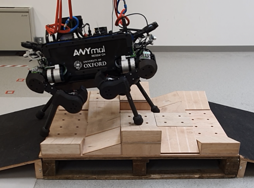
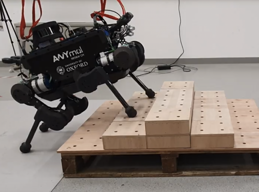
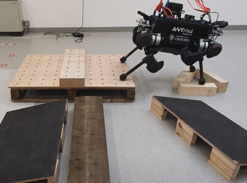
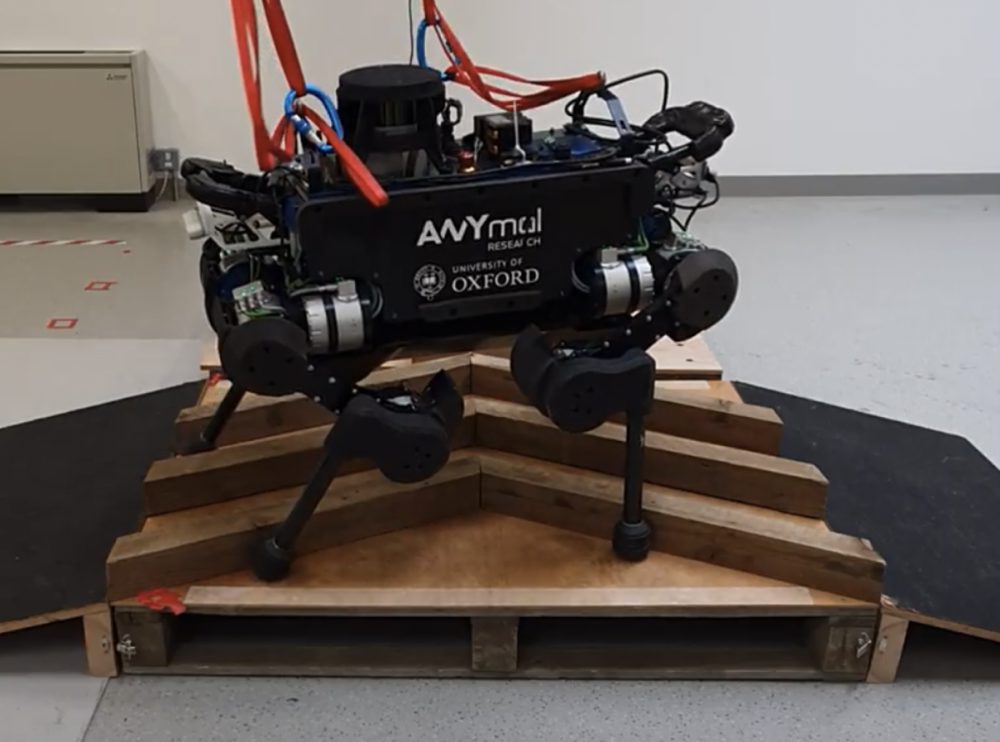
Figure 1: ANYmal B quadruped used to perform experiments on different terrains using our RLOC framework. Overview video can be found at: https://youtu.be/GTI-0gl6Hg0.

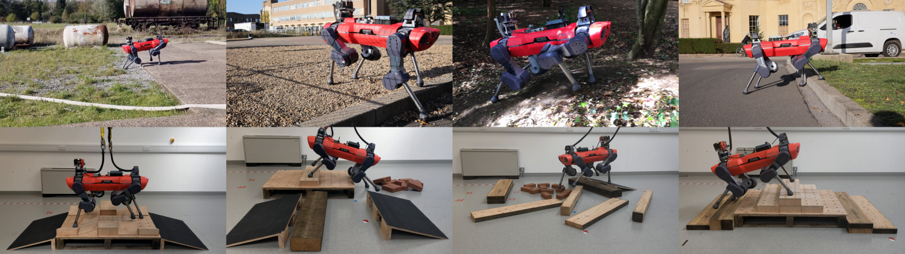
Figure 2: ANYmal C quadruped used to perform experiments on different terrains outdoors; on hard, grassy and muddy terrain also including slopes, and indoors; similar to the experiments performed using ANYmal B. The policies trained using ANYmal B were transferred to ANYmal C without retraining. The video clips of the demonstrations are provided in Movie S6.

The control of such underactuated robotic systems is an active area of research.

Approaches based on whole-body trajectory optimization such as contact-implicit optimization (CIO) [5] can generate complex multi-contact motions but often remain too computationally extensive to be used online. More recent works based on differential dynamic programming (DDP) algorithms [6, 7] enable efficient computation of whole-body motions suitable for online execution. These methods, however, are still under development, and their effectiveness on physical systems and complex environments is yet to be demonstrated.

A rich body of work has focused on using simplified dynamic models which capture only the main dynamics of the system so as to achieve a balance of computational complexity [8]. Such models are also known as templates and are typically lower dimensional than the full (whole-body) model, and also linear with respect to the states of the system; the mechanism that relates them back to the whole-body model is instead usually called the anchor. Examples of templates include the linear inverted pendulum (LIP) [9] and the spring-loaded inverted pendulum (SLIP) [10], and their derived variants [11].

For the development of robust model-based controllers, the synthesis of stability criteria based on ground reference points (2D points on a flat ground plane) such as the zero moment point (ZMP) [12] and the instantaneous capture point (ICP) [13] is also introduced into the control problem. The templates can be seen as a way to constrain the admissible domain of such ground reference points. In this regard, the balancing problem for legged robots can be translated into an inclusion problem that requires the reference point to belong to its admissible region, i.e. the support region, for the robot to be stable. In this way, a measure of robustness, the stability margin, can be defined as the distance between the reference point and the edges of its admissible region.

Often, simplified models and ground reference points are limited to flat terrain and their descriptive accuracy deteriorates when applied to environments with complex geometry. For such multi-contact conditions, the centroidal dynamics model [14] is widely used. It represents the system in a compact manner such that it focuses on the inputs (contact wrenches) and the outputs (center of mass accelerations) in the task space of the robot discarding the intermediate joint-space physical quantities. In this case, the reference point for evaluating stability can be described by a 6-dimensional wrench. Therefore, for evaluation of stability, templates that illustrate suitable 6D admissible regions need to be defined [15]. Despite their low dimensionality, such simplified models are still typically too numerically inefficient to be employed in the robot’s real-time control loop. An alternative approach is to evaluate the stability of the robot directly using the contact forces [16]. This method, however, necessitates introduction of the contact force variables in the locomotion problem thereby adding to computational delays which result in reduced reactive control.

Recent research on model-predictive control (MPC) based strategies have demonstrated perceptive locomotion over uneven terrain [17, 18]. These controllers, however, often employ system model approximations, due to which, the potential of the physical robot is not fully exploited.

Moreover, these methods require exhaustive tuning of planning and control parameters, requiring considerable development time.

Alternatively, an entirely different approach has focused on investigating solutions which can perform a direct mapping between sensory information to desired control signals with minimal computational overhead. Model-free data-driven techniques such as RL have introduced promising substitutes to model-based control methods, and achieved highly dynamic and robust locomotion skills on complex legged robot systems such as ANYmal B [19, 20, 21], Laikago [22] and Cassie [23]. The major challenge of using RL lies in the fact that training these methods is extremely sample inefficient, especially for high-dimensional problems such as legged locomotion. When applied to a robot such as ANYmal B, the vast exploration space associated with an RL policy, not only necessitates considerable amount of training samples, but also implies that without precise reward function tuning, the RL agent could converge towards an undesired control behavior. As an alternative, a guided policy exploration approach, such as guided policy search (GPS) [24], which relies on utilizing model-based control solutions in conjunction with data-driven policy optimization can be employed to direct policy convergence and increase sample efficiency.

The possibility of damaging the robotic system itself and the environment of operation during policy exploration necessitates the use of simulation platforms. Ease of access to physics simulators, and the ability to execute simulations much faster than real-time, makes this approach appealing for training RL policies. However, the inaccuracy associated with the complex dynamics that are hard to model in simulation often affect the performance of RL policies when deployed onto real systems.

Although there have been works where training was done on the real system itself [25, 26], this has been appropriate for simpler and inherently stable robots which cannot be employed for training complex quadrupedal systems such as the ANYmal robots.

To address the reality gap problem, more accurate models of the training environment can be directly introduced into the simulators. For example, Hwangbo et al. introduced an actuator network [19] to model the dynamics of the physical actuators and further performed ablation studies to justify the necessity for accurate models to achieve simulation-to-real transfer. Moreover, for a training environment, it is very likely that not all the dynamics can be precisely modeled. As a solution, domain randomization [27] techniques have been used to train policies which are robust to unaccountable factors [19, 21].

Most of the above mentioned RL research focuses on quadrupedal locomotion on flat ground, overlooking the primary purpose of quadrupedal systems – mobility over rough terrain.

Tsounis et al. presented an approach for terrain-aware gait planning and control using RL for the ANYmal B quadruped [28]. Tsounis et al. used a hierarchical approach to plan gaits suitable for navigation to a desired goal position, and then performed whole-body control, both using RL. However, different gait planning policies were trained for different terrains, while sim-to-real transfer was not addressed. Lee et al. presented an RL based approach for quadrupedal locomotion over challenging terrains [29], however, this work only focused on use of proprioceptive feedback for locomotion without explicitly processing terrain information. Recently, Miki et al. demonstrated robust and perceptive locomotion skills in unstructured environments [30]. Their control framework exhibited impressive terrain-adaptive behavior even with invalid exteroceptive feedback. This work, however, did not demonstrate significant robustness to variations in kinematic and dynamic properties. For transfer to a different robot not introduced during training, their proposed approach is expected to require further retraining.

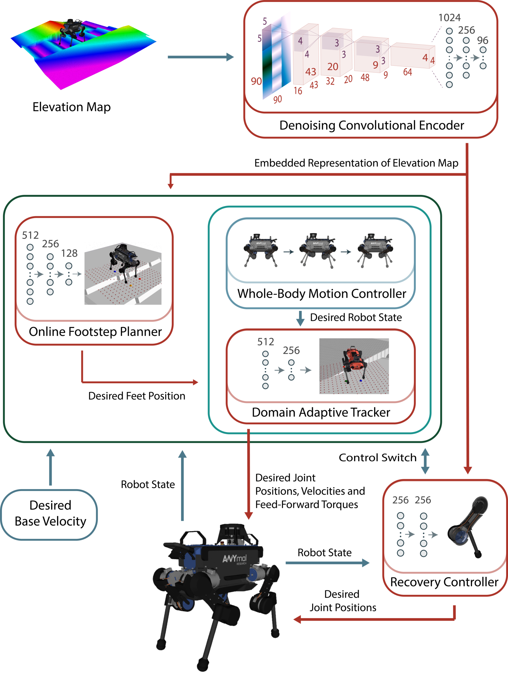
Figure 3: Overview of the proposed control framework - RLOC. We use an online footstep planning RL policy to generate desired feet positions which are tracked using a model-based whole-body motion controller. In order to perform accurate tracking even in case of changes in robot dynamics, we introduce a domain adaptive tracking policy to generate feed-forward corrective torques. Furthermore, in order to exhibit a quick response to external perturbations, we introduce a recovery control policy which generates low-level joint position commands.

In this work, we propose a unified RL and optimal control (OC) based terrain-aware legged locomotion framework as illustrated in Fig. 3. We train a footstep planning RL policy which maps the robot state and terrain information to desired feet positions. In order to track these positions, we extend the dynamic gaits motion controller of Bellicoso et al. [31] to enable foothold tracking over non-flat terrain. This forms the core of our locomotion framework. In order to account for changes in physical parameters and actuation dynamics, we train a domain adaptive tracking policy which introduces corrective feed-forward joint torques for accurate tracking of the trajectories generated by the motion controller. Furthermore, to enable recovery to a stable state upon perturbations or unexpected events like foot slippage, we train an RL policy to generate low-level joint position commands such that during unstable motions, the RL policy stabilizes the robot and then the control switches back to the footstep planning and tracking modules. A video overview of our proposed framework is presented in Movie 1.

Our main contribution with this work is realizing a modular framework which combines RL and OC based approaches to obtain a system-adaptive control solution for perceptive and dynamic robotic locomotion. The adaptive characteristic further facilitates robustness to variations in dynamic and kinematic properties of the system. The key elements of this work thus include (1) Presenting a training approach for obtaining a perceptive footstep planning policy which employs a model-based dynamic motion controller. This setup enables us to generate valid dynamic motion plans while ensuring the obtained policy adapts to and exploits the domain largely described by the characteristics of the motion controller. (2) Obtaining a domain adaptive tracking policy which can be utilized to address system modeling inaccuracies during whole-body motion tracking. This allows us to use a model-based controller on a robot where the modeled characteristics differ from the actual kinematic and dynamic properties of the system. This further enables us to perform dynamics randomization while training the footstep planning policy without requiring retuning of the motion controller. (3) Demonstrating zero-shot generalization to a domain not explicitly modeled during training. For this, we show transfer of our framework to the physical ANYmal C robot despite having been trained in a simulator with ANYmal B.

Our framework allows for high-level tracking of reference base velocity commands over complex uneven terrain, enabling the robot to be operated either by a user (through a remote control) or a higher-level goal planner. We evaluate the performance of RLOC on a wide range of simulated terrains and present the results for the ANYmal B and C quadrupeds. We further transfer RLOC on to the real robots.

II Preliminaries

II-A System Model

A general quadrupedal robotic system can be modeled as a floating base $B$ with four actuated limbs attached to it. The robot state can be described w.r.t. a global inertial reference frame $W$ where the base position is expressed as ${}_{W}r_{\,WB}\in\mathbb{R}^{3}$, and the orientation, $\mathrm{q}_{WB}\in\mathit{SO}(3)$, is represented using Hamiltonian unit quaternions with a corresponding rotation matrix $\mathbf{R}_{WB}\in\mathit{SO}(3)$. We assume that the $z$-axis of $W$, $\mathbf{e}_{z}^{W}$, aligns with the gravity axis. The angular positions of the rotational joints in each of the limbs are described as a vector $\mathrm{q}_{j}\in\mathbb{R}^{n_{j}}$. For the ANYmal robots, $n_{j}=12$. The linear and angular velocities of the base w.r.t. the global frame are written as ${}_{W}\mathrm{v}_{WB}\in\mathbb{R}^{3}$ and ${}_{W}\mathrm{\omega}_{\,WB}\in\mathbb{R}^{3}$ respectively. The generalized coordinates and velocities are thus stacked as vectors $\mathrm{q}$ and $\mathrm{u}$ where

$$\mathrm{q}=\begin{bmatrix}{}_{W}r_{\,WB}\\ \mathrm{q}_{WB}\\ \mathrm{q}_{j}\end{bmatrix}\in\mathit{SE}(3)\times\mathbb{R}^{n_{j}},\quad\mathrm{u}=\begin{bmatrix}{}_{W}\mathrm{v}_{WB}\\ {}_{W}\mathrm{\omega}_{\,WB}\\ \mathrm{\dot{q}}_{j}\end{bmatrix}\in\mathbb{R}^{6+n_{j}}.$$ (1)

We denote positions of the feet in the global reference frame as ${}_{W}r_{\,WF}\in\mathbb{R}^{3\times n_{f}}$, where $n_{f}=4$ is the number of feet. We additionally define ${}_{W}r_{\,WF_{xy}}\in\mathbb{R}^{2\times n_{f}}$ as a vector of $x$ and $y$ components of the feet positions.

We introduce a horizontal frame $H$ such that ${}_{W}r_{\,WH}={}_{W}r_{\,WB}$ and $\mathbf{R}_{WH}=\mathbf{R}_{WB_{z}}$, where $\mathbf{R}_{WB_{z}}$ is the $z$ decomposition of the base rotation matrix which can also be expressed as $\mathbf{R}_{WB}=\mathbf{R}_{WB_{z}}\mathbf{R}_{WB_{y}}\mathbf{R}_{WB_{x}}$. The frame $H$ can thus be interpreted as having the same translation as the robot base frame $B$ w.r.t. the global inertial reference frame, but rotation in the frame $H$ is only permissible along $\mathbf{e}_{z}^{H}$, implying that the gravity axis always aligns with the $z$-axis of frame $H$. Additionally, the yaw rotation of frame $H$ also always aligns with the yaw rotation of frame $B$. We then represent the local robocentric terrain elevation in the horizontal frame as $\mathbf{M}_{H}:\mathbb{R}^{2}\times\mathbb{R}\rightarrow\mathbb{R}^{91\times 91}$, an elevation map corresponding to an area of $1.8\times 1.8\,$${\mathrm{m}}^{2}$ and a resolution of $0.02\text{\,}\mathrm{m}$.

The quadrupedal system is actuated using the joint control torques $\tau_{j}\in\mathbb{R}^{n_{j}}$. These torques are computed at the actuator level using an impedance control model written as

$$\tau_{j}=K_{p}(\mathrm{q}^{\ast}_{j}-\mathrm{q}_{j})+K_{d}(\mathrm{\dot{q}}^{\ast}_{j}-\mathrm{\dot{q}}_{j})+\tau_{j_{FF}}$$ (2)

where $K_{p}$ and $K_{d}$ refer to the position and velocity tracking gains respectively, $\mathrm{q}^{\ast}_{j}$ is the vector representing desired joint positions, $\mathrm{\dot{q}}^{\ast}_{j}$, the desired joint velocities, and $\tau_{j_{FF}}$ refers to the feed-forward joint torques.

Note that, for concise presentation, we will assume that all of the translations and rotations are measured and expressed in the global reference frame $W$ unless otherwise stated. In this regard, for the rest of the manuscript, the notation ${}_{W}r_{WB}$ will be shortened to $r_{B}$, $\mathbf{R}_{WB}$ to $\mathbf{R}_{B}$, and similarly for all the other introduced notations.

II-B Motion Parameterization

The motion of the quadrupedal system is expressed in terms of the center of mass (CoM) and feet motions. In consistency with the definitions introduced in [31], we represent the CoM motion plan in the form of a sequence of quintic splines where the $j$-th spline for the $x$ component is represented as

$$\begin{split}&x(t)=\alpha^{x}_{j5}t^{5}+\alpha^{x}_{j4}t^{4}+\alpha^{x}_{j3}t^{3}+\alpha^{x}_{j2}t^{2}+\alpha^{x}_{j1}t+\alpha^{x}_{j0}\\ &\qquad=[t^{5}\quad t^{4}\quad t^{3}\quad t^{2}\quad t\quad 1]\\ &\qquad\quad\cdot[\alpha^{x}_{j5}\quad\alpha^{x}_{j4}\quad\alpha^{x}_{j3}\quad\alpha^{x}_{j2}\quad\alpha^{x}_{j1}\quad\alpha^{x}_{j0}]^{T}\\ &\qquad=\eta^{T}(t)\alpha^{x}_{j}.\end{split}$$ (3)

The spline $j$ corresponds to a duration of $\Delta\,t_{j}$ such that $t\in[\overline{t},\,\overline{t}+\Delta\,t_{j}]$. Here $\overline{t}$ refers to the total elapsed time of the motion described by $j-1$ splines. We therefore express the CoM position, $\mathrm{p}_{CoM}\in\mathbb{R}^{3}$, as $\mathrm{p}_{CoM}=\mathbf{K}(t)\alpha_{j}$ where

$$\mathbf{K}(t)=\begin{bmatrix}\eta^{T}(t)&0&0\\ 0&\eta^{T}(t)&0\\ 0&0&\eta^{T}(t)\end{bmatrix},$$ (4)

and $\alpha_{j}=[{\alpha_{j}^{x}}^{T}\quad{\alpha_{j}^{y}}^{T}\quad{\alpha_{j}^{z}}^{T}]^{T}$. The CoM velocity is thus represented as $\mathrm{\dot{p}}_{CoM}=\mathbf{\dot{K}}(t)\alpha_{j}$, and the acceleration as $\mathrm{\ddot{p}}_{CoM}=\mathbf{\ddot{K}}(t)\alpha_{j}$.

We parameterize the feet motions based on their contact state given by the vector $\mathrm{c}_{F}\in\left\{0,0.5,1\right\}^{4}$ where an open-contact is represented by 0 and close-contact (with zero foot velocity) by 1. Depending on the terrain, there remains a possibility of foot slippage i.e. a close-contact with non-zero foot velocity. This contact-uncertainty state is therefore denoted by 0.5. For the purpose of motion planning, we only consider the open (0) and close (1) contact states. The contact-uncertainty state is instead utilized for adapting the joint PD control gains during motion tracking. This is detailed in Section III-B.

We define the swing phase, $\Phi_{o,i}$, for foot $i\in\{0,1,2,3\}$ to correspond to the foot motion where $\mathrm{c}_{F,i}=0$. Conversely, the stance phase, $\Phi_{c,i}$, corresponds to the motion where $\mathrm{c}_{F,i}=1$. Both the swing and stance phases can be described by the tuple

$$\Phi=\langle r_{F}^{l},r_{F}^{d},r_{F}^{h},\mathrm{c}_{F},t_{F}^{l},t_{F}^{d},v^{l}_{F},v^{d}_{F}\rangle$$ (5)

where $r_{F}^{l}$, $r_{F}^{d}$ and $r_{F}^{h}$ refer to the vectors describing the feet lift-off, touch-down and clearance positions respectively. The foot clearance position represents the maximum $r_{F_{z},i}$ during the given phase. For $\Phi_{o,i}$, $t_{F,i}^{l}$ is the time elapsed since previous lift-off and $t_{F,i}^{d}$ is the time until touch-down. For $\Phi_{c,i}$, $t_{F,i}^{l}$ refers to the time until lift-off and $t_{F,i}^{d}$ is the time elapsed since previous touch-down. $v^{l}_{F}$ and $v^{d}_{F}$ refer to the feet lift-off and touch-down velocities respectively. Additionally, for $\Phi_{c,i}$, we consider $r_{F}^{l}=r_{F}^{d}=r_{F}^{h}$.

II-C Reinforcement Learning

The problem of sequential decision making can be formulated in the framework of a discrete time Markov decision process (MDP) [32]. An MDP is defined by the tuple - $\langle S,A,R,P,\mu\rangle$, where $S$ represents a set of states, $A$ a set of actions, $R:S\times A\times S\rightarrow\mathbb{R}$ the reward function, $P:S\times A\times S\rightarrow\left[0,1\right]$ the state transition probability, and $\mu$ the initial state distribution. In the context of deep RL, as utilized in our work, an RL agent described in this MDP framework interacts with an environment based on a policy $\pi:S\rightarrow\mathcal{P}\left(A\right)$ which is modeled as a neural network. This policy can be defined as a function mapping states to probability distributions over actions such that $\pi\left(a|s\right)$ denotes the probability of selecting action $a$ in state $s$. The objective of the RL agent is to then obtain a policy $\pi_{\theta}$ for parameters $\theta$ in order to maximize the expected cumulative discounted return,

$$J\left(\pi\right)\doteq\underset{\mathcal{T}\sim\pi_{\theta}}{\text{{E}}}\left[\sum_{t=0}^{\infty}{{\gamma}^{t}R\left({s}_{t},{a}_{t},{s}_{t+1}\right)}\right]\text{,}$$ (6)

where $\gamma\in\left[0,1\right)$ is the discount factor and $\mathcal{T}$ denotes a trajectory dependent on $\pi_{\theta}$.

III Methodology

We present a modular terrain-aware quadrupedal planning and control framework for locomotion over uneven terrain. We propose a footstep planner which utilizes the proprioceptive and exteroceptive information to generate the desired feet touch-down positions, ${r_{F}^{d}}^{\ast}$, that are tracked during the immediate swing phases. The footstep planner is sequentially evaluated after each of the previous four swing phases are executed, completing a gait stride. The desired footholds are thus updated after each gait stride at the instance when each of the feet is in stance phase, $\mathrm{c}_{F}=\overrightarrow{1}_{F}$ where $\overrightarrow{1}_{F}\in\mathbb{R}^{4}$ is a vector of ones. The dynamic gaits motion controller, which serves as a motion planner and whole-body controller, is then employed to generate and track the desired CoM and feet motion plans. The whole-body tracking of motion plans occurs at $400\text{\,}\mathrm{Hz}$, while the motion planning optimization is performed in parallel to the control thread and a new optimization problem is run everytime a solution is found.

The domain adaptive tracker, also executed at $400\text{\,}\mathrm{Hz}$, is trained to introduce additive deviations to the feed-forward joint torques generated by the motion controller, $\tau_{j_{FF}}$. These additive deviations, $\delta\tau_{j_{FF}}$, are included in the impedance controller shown in eq. 2 and account for discrepancies in the modeled and actual system dynamics. Finally, the recovery controller, running at $400\text{\,}\mathrm{Hz}$, is activated to perform joint position control when a robot state is encountered such that the motion controller becomes unstable and is unable to execute a state recovery behavior.

We employ this modular control architecture for following reasons:

1. The individual trained modules can be precisely tuned to adapt to different tasks. For example, transferring the framework for use on a quadruped with significantly larger mass would only require adapting either the motion controller or the domain adaptive tracker. This, in fact, also allows us to perform a zero-shot transfer from the simulated ANYmal B training domain to the physical ANYmal C.

2. In our preliminary experiments, we observed that training a terrain-aware locomotion policy which outputs desired joint position commands required comprehensive tuning of the RL environment parameters, without which, the network often failed to learn, resulting in a behavior where the robot would not respond to velocity commands, instead, would stand in place. This observation significantly contributed towards our modular control architecture design. A modular framework enabled us to perform easier tuning of individual components. The contributions of each of the modules are detailed in Section V.

3. Distributing the planning and control tasks between the RL footstep planner and the model-based motion controller enabled us to obtain a footstep planner which was able to generalize to wide range of terrains in less than $32\text{\,}\mathrm{h}$ of total training. In contrast, the gait planner of DeepGait [28] required $82\text{\,}\mathrm{h}$ of training time for each of the terrains. Moreover, the gait controller of DeepGait required further $116\text{\,}\mathrm{h}$ of training time for each of the uneven terrains, and an additional $58\text{\,}\mathrm{h}$ of training for locomotion on flat-ground, totaling the training time to approximately $454\text{\,}\mathrm{h}$ for locomotion over three different terrains: Flat-World, Temple-Ascent, and Random-Stairs (see DeepGait [28]).

An overview of the control framework is presented in Fig. 3. This section details upon each of the modules. We also describe the MDPs for the footstep planner, domain adaptive tracker and the recovery controller in this section. The detailed RL training setups are presented in Section IV.

III-A Elevation Map Encoding

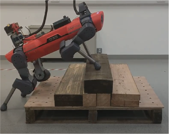
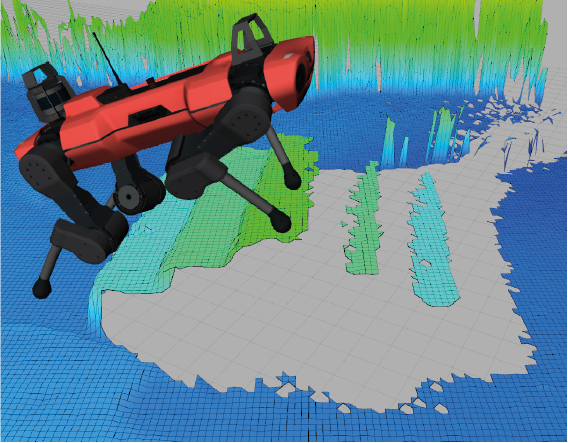
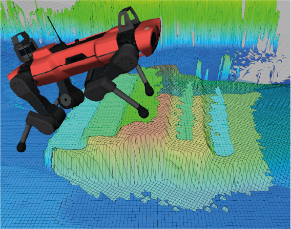
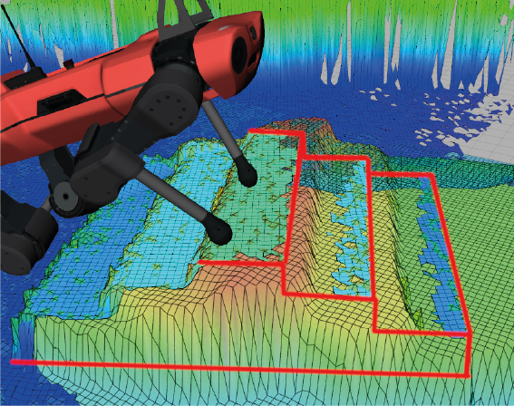
Figure 4: top: Ascending stairs with ANYmal C (left) and the corresponding raw elevation map (right). The unfilled regions in the raw elevation map represent non-observable terrain information which could not be captured by the depth camera on the robot due to occlusions. bottom: Filtered elevation map obtained using nearest-neighbors interpolation (left) and the terrain edges (right).

We extract robocentric terrain elevation, $\mathbf{M}_{H}$, using the elevation mapping framework presented in [33] and embed it to obtain a latent representation, $\mathrm{Z}_{\mathbf{M}_{H}}\in\mathbb{R}^{96}$. This representation is generated by an encoding network, $E_{\mathbf{M}_{H}}$ which is trained using a denoising convolutional auto-encoding strategy. Our motivation for performing this embedding (including the encoding approach) is based on the following reasons:

1. Three of the modules constituting our RLOC framework utilize exteroceptive terrain information. Pre-processing the elevation map to extract terrain features eliminates repeated processing of the elevation map by each of the modules limiting further computational delays.

2. The denoising property of $E_{\mathbf{M}_{H}}$ is relevant to perform a sim-to-real transfer. The elevation map extracted on the physical system is often noisy and contains occlusions that cannot be precisely modeled. An example of this is shown in Fig. 4. This has further been studied in [30]. A nearest-neighbors interpolation technique is employed to obtain a filtered elevation map which often results in distortions (e.g. the edges of the steps are blurred and shifted). The denoising auto-encoding strategy enables extraction of the most relevant terrain features like edges and slopes even with distorted terrain information.

3. A pre-trained terrain feature extractor implies that, during training of RL policies, the RL agent does not need to learn the parameters for the terrain feature extraction block thereby making the training faster while also adapting to a pre-trained encoder which can be shared with multiple modules.

4. Even though different strategies such as fast Fourier transform (FFT) can be employed to compress the elevation map, our work focuses on utilizing deep learning strategies for feature extraction. This enables us to adapt the previously trained network to a diverse class of terrains by retraining the encoder. Additionally, strategies such as transfer learning can be utilized to reduce training complexity. The feature extractor can also be retrained along with an RL policy to adapt to different tasks not introduced during prior training.

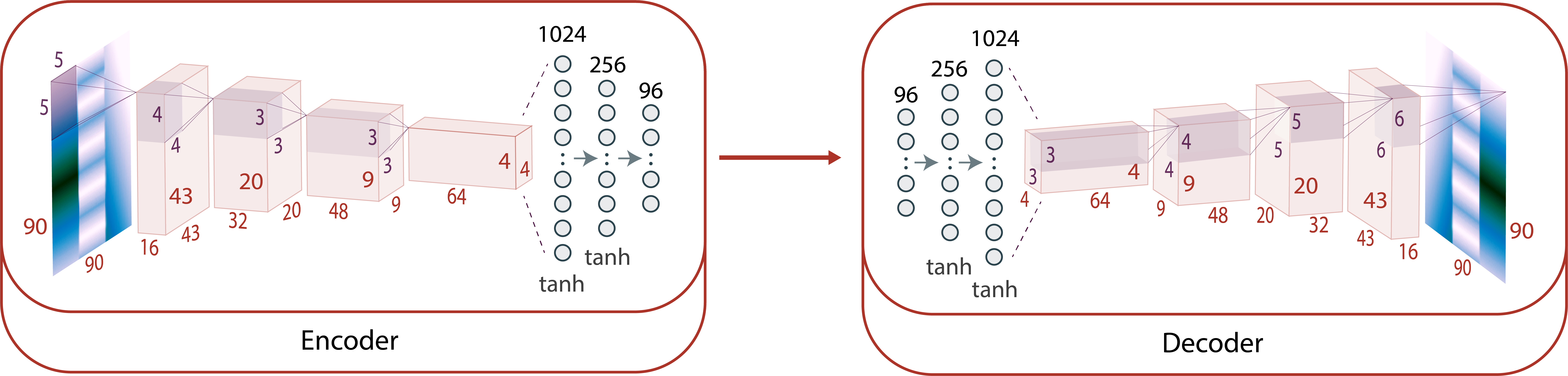
Figure 5: Network architecture of the denoising convolutional autoencoder used to generate an embedded representation of the local elevation map. We use the leaky ReLU activation function for the convolutional layers and the tan hyperbolic activation function for the dense layers.

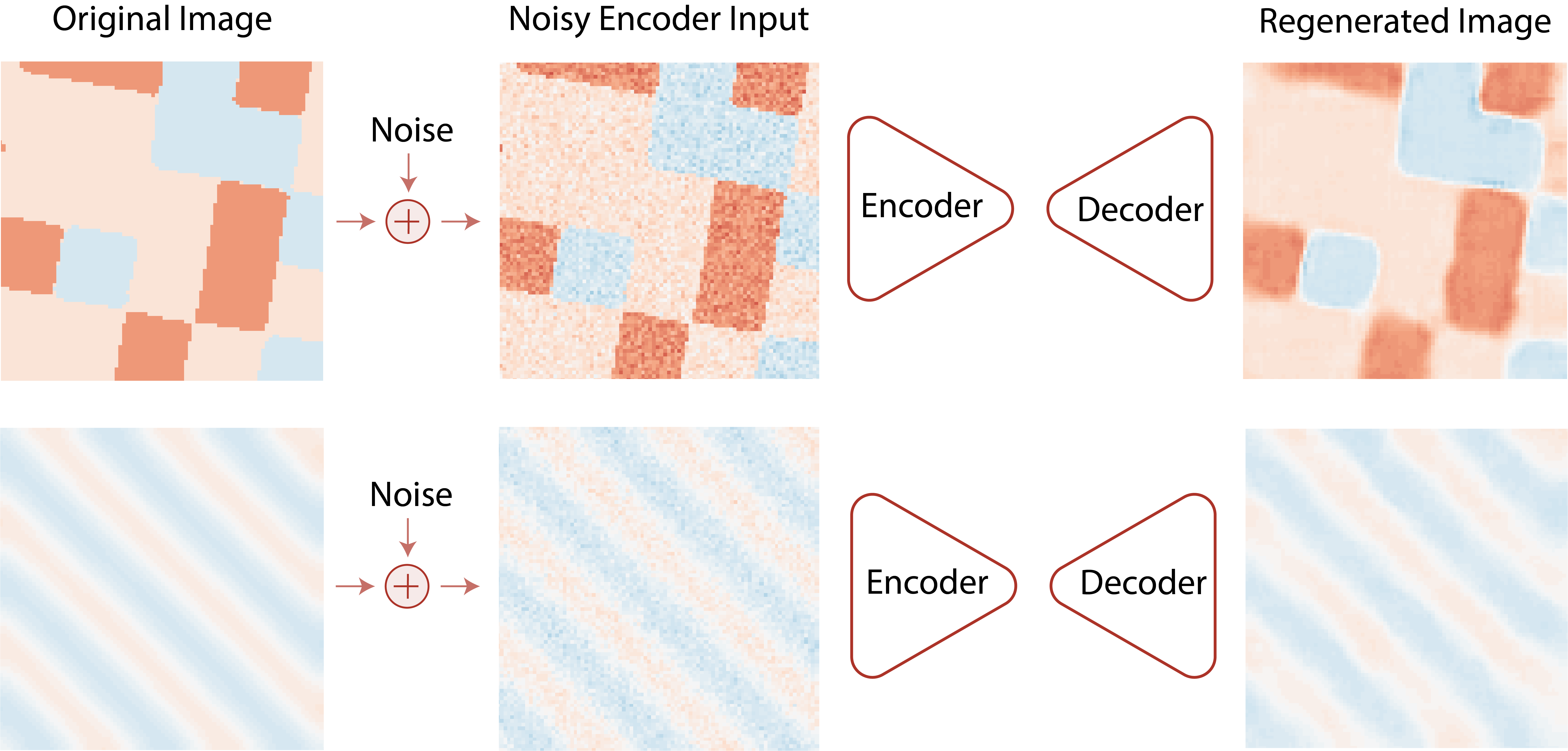
Figure 6: Examples of regeneration of noisy images using our trained autoencoder - top: a patch from the bricks terrain and bottom: a patch from the sine wave terrain.

The architecture of the denoising convolutional auto-encoder is presented in Fig. 5. Note that, while extracting the elevation map, we clip $\mathbf{M}_{H}$ in the range $[-2,2]\,$$\mathrm{m}$. For network training and evaluation stability, we further normalize $\mathbf{M}_{H}$ by performing a scalar division by 2 to obtain $\mathbf{M}_{H}^{n}$ with elements in the range $[-1,1]$. As part of training, our objective is then to learn the weights of the convolutional encoder $E_{\mathbf{M}_{H}}$, such that

$$\mathrm{Z}_{\mathbf{M}_{H}}=E_{\mathbf{M}_{H}}(\mathbf{M}_{H}^{n}+\mathbf{N}_{\mathbf{M}}(\mathbf{M}_{H}^{n}))$$ (7)

where $\mathbf{N}_{\mathbf{M}}$ represents the artificial noise introduced in $\mathbf{M}_{H}^{n}$, and

$${\mathbf{\hat{M}}}_{H}^{n}=D_{\mathbf{M}_{H}}(\mathrm{Z}_{\mathbf{M}_{H}})$$ (8)

where $D_{\mathbf{M}_{H}}$ is the decoder network which maps the latent embedding of $\mathbf{M}_{H}^{n}$ to its approximate reconstruction ${\mathbf{\hat{M}}}_{H}^{n}$. Both $E_{\mathbf{M}_{H}}$ and $D_{\mathbf{M}_{H}}$ are trained together using supervised learning to minimize the reconstruction loss

$$\mathcal{L}_{\mathbf{M}_{H}}=({\mathbf{M}}_{H}^{n}-{\mathbf{\hat{M}}}_{H}^{n})^{2}\,.$$ (9)

The artificial noise, $\mathbf{N}_{\mathbf{M}}:\mathbb{R}^{91\times 91}\rightarrow\mathbb{R}^{91\times 91}$, is expressed as

$$\begin{split}&\mathbf{N}_{\mathbf{M}}(\mathbf{M})=n_{\mathcal{N}}\mathcal{N}_{91\times 91}(0,\,1)\\ &\qquad\qquad+\,(\mathcal{I}({\mathbf{M}},p_{\mathcal{I}})-\mathbf{M})\\ &\qquad\qquad+\,n_{\mathcal{C}}(\mathcal{C}(\mathbf{M},k_{b})-\mathbf{M})\end{split}$$ (10)

where $\mathbf{M}\in\mathbb{R}^{91\times 91}$ is a matrix similar to $\mathbf{M}_{H}^{n}$, $\mathcal{N}$ is the additive Gaussian noise, $\mathcal{I}$ is the impulse noise also know as salt-and-pepper noise, $p_{\mathcal{I}}\sim\mathcal{U}(0,0.05)$ is the probability of introduced impulses sampled uniformly in the range $[0,0.05]$, $\mathcal{C}$ is the 2D convolution function, and $k_{b}\in\mathbb{R}^{3\times 3}$ is the convolutional blurring kernel written as

$$k_{b}=\frac{1}{9}\times\begin{bmatrix}1&1&1\\ 1&1&1\\ 1&1&1\\ \end{bmatrix}\,.$$ (11)

$n_{\mathcal{N}}\sim\mathcal{U}(0,0.05)$ and $n_{\mathcal{C}}\sim\mathcal{U}(0,1)$ are the coefficients for weighting the noise functions.

To train the denoising convolutional autoencoder, we use our terrain generator tool, described in Section IV-A1, to generate $20\times 20\,$${\mathrm{m}}^{2}$ terrains, where each terrain is represented as $\mathbf{T}\in\mathbb{R}^{1001\times 1001}$. These terrains contain objects such as stairs, wave, bricks, planks and unstructured ground. We slice a $91\times 91$ matrix from $\mathbf{T}$ at randomly selected positions and further use data-augmentation techniques such as rotation, mirroring and modifying contrast during training of the autoencoder online. This augmentation is done in parallel to the main training session in a separate thread. Figure 6 shows examples of regeneration of noisy terrain inputs using the trained autoencoder.

III-B Motion Controller

Rudin et al. propose an architecture which allows for direct mapping of proprioceptive and exteroceptive state information to desired joint positions [34]. This, however, often requires exhaustive reward tuning to achieve a desired locomotion behavior [19, 21]. As an alternative, [30] utilizes central pattern generators (CPGs) to achieve an underlying oscillatory behavior for each of the quadrupedal limbs. This architecture enables online adaptation of the locomotion gait while also making the RL training less demanding [35]. In this work, we are driven by the motivation that the proposed framework should be robust to variations in system kinematics and dynamics. For this, we utilize a motion controller to generate and track base and feet motion plans for traversal over uneven terrain. The desired feet positions are instead generated by the RL footstep planner described in Section III-C. This eliminates the need for the RL agent to perform motion control thereby simplifying training. Additionally, the model-based motion control architecture ensures that safety-critical constraints such as joint kinematic limits and peak joint torques are still enforced by the low-level controller. The system-adaptive property is then induced by the domain adaptive tracker presented in Section III-D.

In this work, we extend the dynamic gaits motion controller of Bellicoso et al. [31] to generate CoM and feet motion plans for traversal over uneven terrain. The CoM motion plan is generated by solving a nonlinear optimization problem to track the velocity command, $\mathbf{c}^{\ast}$, for a time horizon $t_{H}^{c}$. This time horizon corresponds to the period of the active locomotion gait. We introduce a control frame $C$ such that $r_{C}=r_{B}$, $\mathbf{R}_{C_{z}}=\mathbf{R}_{B_{z}}$, and $\mathbf{e}_{z}^{C}$ aligns with the normal of the estimated terrain plane $\mathbf{e}_{z}^{T}$. The velocity command is therefore expressed in the control frame as

$$\mathbf{c}^{\ast}=[\mathrm{v}_{x}^{\ast}\mathbf{e}_{x}^{C}\quad\mathrm{v}_{y}^{\ast}\mathbf{e}_{y}^{C}\quad\mathrm{\omega}_{z}^{\ast}\mathbf{e}_{z}^{C}]^{T}$$ (12)

where $\mathrm{v}_{x}^{\ast}$ and $\mathrm{v}_{y}^{\ast}$ are the desired heading and lateral velocities expressed along $\mathbf{e}_{x}^{C}$ and $\mathbf{e}_{y}^{C}$ respectively, and $\mathrm{\omega}_{z}^{\ast}$ is the desired yaw rate around the vertical axis $\mathbf{e}_{z}^{C}$.

The motion controller employs a quadratic programming (QP) based foothold planning module to generate the desired feet touch down positions, ${r_{F}^{d}}^{\ast}$. This is replaced by the RL footstep planner in our proposed framework. The vertical component of the desired touch down positions, ${r^{d}_{F_{z}}}^{\ast}$, is directly extracted from the terrain plane estimate for each swing phase. The contact scheduler module of the motion controller manages the feet contact events for a full stride of an active gait. It generates the lift-off, $t_{F}^{l}$, and touch-down, $t_{F}^{d}$, timings for the feet swing and stance phases. The $\Phi_{o}$ and $\Phi_{c}$ thus obtained is used to generate feet motion plans to track ${r_{F}^{d}}^{\ast}$.

A detailed description of the modifications introduced in the original motion controller is provided in the Appendix.

The generated reference motion plans are tracked using a whole-body controller [36] based on a hierarchical QP optimization framework to optimize for the generalized accelerations $\mathrm{\dot{u}}$ and feet contact forces to generate the feed-forward torques $\tau_{j_{FF}}$. The impedance control torques are then computed by extracting the desired joint positions, $\mathrm{q}^{\ast}_{j}$, and joint velocities, $\mathrm{\dot{q}}^{\ast}_{j}$, from the feet motion plans using inverse kinematics.

The work of Jenelten et al. on locomotion over slippery surfaces [37] proposes the use of impedance gains depending on the feet contact-states. For a foot $i$, the gains are selected according to the rule

$$K_{p,d}^{\mathrm{c}_{F,i}=0.5}>\!>K_{p,d}^{\mathrm{c}_{F,i}=1}>K_{p,d}^{\mathrm{c}_{F,i}=0}$$ (13)

such that, in the contact-uncertainty state $\mathrm{c}_{F,i}=0.5$, the high gains used for joints in the leg containing the foot $i$ prevent further leg slippage due to increased stiffness. For detailed description, we defer the reader to the original work. We use this approach of adaptive impedance for whole-body tracking of the reference motion plans in RLOC.

III-C Footstep Planner

Approximating the perceptive footstep planning policy using a neural network implies that we can directly map the exteroceptive and proprioceptive robot state information to desired feet positions. This rids us of the need for computationally exhaustive task of combinatorial search among a large space of feasible footstep plans. Additionally, as presented in Section V-A, training the footstep planner using deep RL enables natural emergence of planning behavior learned through interactions with the environment of operation. This offers better performance for traversal over unstructured terrains compared to a baseline sampling-based perceptive footstep planner.

Computing new set of desired feet positions after each gait stride, specifically after each of the previous four feet swing phases have been executed, allows us to formulate the problem of footstep planning as a sequential MDP. In particular, we represent the problem as an infinite-state space and infinite-action space MDP.

III-C1 State and Action

We define the MDP state as a tuple $\mathbf{s}_{f}:=\langle s_{R},s_{v},s_{j},s_{c},s_{M}\rangle$, and the action $\mathbf{a}_{f}:=\langle{}_{H}r_{H{F_{xy}}}^{\ast}\rangle$. The state $\mathbf{s}_{f}\in\mathbb{R}^{204}$ comprises terms representing robot base orientation $s_{R}\in\mathbb{R}^{3}$, base linear and angular velocities $s_{v}\in\mathbb{R}^{6}$, sparse representation of history of joint positions and velocities $s_{j}\in\mathbb{R}^{96}$, desired base velocity $s_{c}\in\mathbb{R}^{3}$, and an embedded representation of the robocentric elevation map $s_{M}\in\mathbb{R}^{96}$. The exact definitions of the footstep planner (FP) state terms are provided in Table I. The action $\mathbf{a}_{f}\in\mathbb{R}^{8}$ comprises the desired foothold locations, ${}_{H}r_{H{F_{xy}}}^{\ast}$, for each of the four feet represented in the horizontal frame. The $z$ components of the desired feet positions, ${}_{H}r_{H{F_{z}}}^{\ast}$, are directly extracted from $\mathbf{M}_{H}$. Therefore, the desired feet positions, ${}_{H}r_{HF}^{\ast}$, measured and expressed in horizontal frame can be transformed into the world frame representation using the transformation

$$r_{F,i}^{FP}=(\mathbf{R}_{H})\;({}_{H}r_{HF,i}^{\ast})\ +\ r_{B}$$ (14)

for foot $i$. The feet positions generated by the footstep planner, $r_{F}^{FP}$, are then forwarded to the dynamic gaits motion controller.

TABLE I: State term definitions for the footstep planner MDP. Here, $t$ refers to the current measurement and the duration between $t-1$ and $t$ corresponds to $2.5\text{\,}\mathrm{ms}$.

FP State

$s_{R}=\mathbf{e}_{z}^{B}$

$s_{v}=[(\mathbf{R}_{B}^{T}\mathrm{v}_{B})^{T}\quad(\mathbf{R}_{B}^{T}\mathrm{\omega}_{B})^{T}]^{T}$

$s_{j}=[{\mathrm{q}_{j}}_{t}^{T}\ \ {\mathrm{q}_{j}}_{t-5}^{T}\ \ {\mathrm{q}_{j}}_{t-10}^{T}\ \ {\mathrm{q}_{j}}_{t-50}^{T}\ \ {\dot{\mathrm{q}}_{j}}{}_{t}^{T}\ \ {\dot{\mathrm{q}}_{j}}{}_{t-5}^{T}\ \ {\dot{\mathrm{q}}_{j}}{}_{t-10}^{T}\ \ {\dot{\mathrm{q}}_{j}}{}_{t-50}^{T}]^{T}$

$s_{c}=\mathbf{c}^{\ast}$

$s_{M}=\mathrm{Z}_{\mathbf{M}_{H}}$

Note that, we introduce the history of joint states in the state space to infer the active locomotion gait. The different gaits result in different stability margin [38, 39], a metric introduced in the reward function to assess the dynamic stability of the robot. This implies that the desired feet positions generated by the footstep planner depend on the gait in use. The state space is thus required to contain information relating to the robot locomotion gait.

III-C2 Reward Function

The reward function in the MDP formulation encourages stable dynamic locomotion over uneven terrain in order to track a desired base velocity command while minimizing energy consumption. During execution of the sequential footstep planning MDP in an episodic framework, the planning state transition, ${\mathbf{P}_{f}}_{n}:=\langle{\mathbf{s}_{f}}_{n},{\mathbf{a}_{f}}_{n},{\mathbf{s}_{f}}_{n+1}\rangle$, is only observed after the motion plans for each of the feet are executed. The tracking of these motion plans is instead performed at each control step executed at $400\text{\,}\mathrm{Hz}$. Therefore, each $\mathbf{P}_{f}$ in the footstep planning MDP comprises several control steps. The control behavior observed within these state transitions is still relevant to assess the performance of the footstep planner especially pertaining to velocity tracking and foot slippage. In this regard, our reward function includes a running reward term, $\mathbf{r}_{F}^{\mathrm{r}}\in\mathbb{R}$, accumulated over the control horizon for each $\mathbf{P}_{f}$, and a final reward term $\mathbf{r}_{F}^{\mathrm{f}}\in\mathbb{R}$, computed after a state transition is observed. The reward function can then be expressed as

$$\mathbf{r}_{F}=\mathbf{r}_{F}^{\mathrm{f}}+\frac{1}{(n+1)_{t}-(n_{t}+1)}\left({{\sum}}_{t=n_{t}+1}^{(n+1)_{t}}{\mathbf{r}_{F}^{\mathrm{r}}}_{t}\right)$$ (15)

where $n_{t}$ corresponds to the control step at which state $\mathbf{s}_{f_{n}}$ is observed. The duration between $t=n_{t}+1$ and $t=(n+1)_{t}$ is not fixed and depends upon the touch-down and lift-off timings. We express the running reward at control step $t$ as

$${\mathbf{r}_{F}^{\mathrm{r}}}_{t}=8{\mathbf{r}_{v}}_{t}-0.016d_{f}{\mathbf{r}_{\tau}}_{t}-2.5d_{f}{\mathbf{r}_{\mu}}_{t}+4{\mathbf{r}_{m}}_{t}$$ (16)

comprising the velocity tracking reward $\mathbf{r}_{v}$, control joint torque penalty $\mathbf{r}_{\tau}$, feet slippage penalty $\mathbf{r}_{\mu}$, and the stability margin reward $\mathbf{r}_{m}$. The weighting factor $d_{f}\in[0,1]$ corresponds to the training curriculum and is increased as training progresses to fine tune the behavior of the RL agent. We update the curriculum factor after each policy iteration by the rule $d_{f_{k+1}}\leftarrow{d}_{f_{k}}^{0.9986}$ where $k$ refers to the policy iterations and $d_{f_{0}}=0.02$. The final reward is represented as

$$\mathbf{r}_{F}^{\mathrm{f}}=-2d_{f}\mathbf{r}_{n}-1d_{f}\mathbf{r}_{e}-2.5d_{f}\mathbf{r}_{\mu}+4\mathbf{r}_{m}+2\mathbf{r}_{h}$$ (17)

comprising the penalty for deviation from nominal footholds $\mathbf{r}_{n}$, reward for distance from terrain edges $\mathbf{r}_{e}$, feet slippage penalty $\mathbf{r}_{\mu}$, the robot stability margin reward $\mathbf{r}_{m}$ based on [39], and the feet height reward relating to the closeness to the nominal feet height $\mathbf{r}_{h}$. The definitions for the reward terms are presented in Table II.

TABLE II: Reward term definitions for the footstep planner MDP. Here $K$ refers to the logistic kernel defined as ${K(x):=({{e^{x}+2+e^{-x}}})^{-1}}$. $\mathcal{S}_{m}$ is the function mapping robot state information to the robot stability margin, $N_{F}$ represents the feet contact normals, $\overrightarrow{F}_{B}$ represents the external force on base, $\overrightarrow{\tau}_{B}$ is the external torque applied on base, $\mathbf{T}_{\mu}$ is the terrain friction coefficient, and $\mathbf{C}_{\mathbf{M}}$ maps the foot position to a cost describing the distance of the foot from the terrain edges. The functions $\mathcal{S}_{m}$ and $\mathbf{C}_{\mathbf{M}}$ are detailed in the Appendix. ${{}_{H}r^{n}_{HF_{z}}}$ is the $z$ component of the nominal feet positions.

FP Rewards

$\mathbf{r}_{v}=K\left(5\|\mathbf{c}^{\ast}-\mathbf{c}\|^{2}\right)$

$\mathbf{r}_{\tau}=\|\tau_{j}\|^{2}$

$\mathbf{r}_{\mu}=\sum{\|\dot{r}_{F,i}\|},\ \ \forall{i},\mathrm{c}_{F,i}=1,i\in\{0,1,2,3\}$

$\mathbf{r}_{m}=\mathcal{S}_{m}(\mathrm{q},\mathrm{{u}},\mathrm{\dot{u}},\mathrm{r}_{F},\mathrm{c}_{F},N_{F},\overrightarrow{F}_{B},\overrightarrow{\tau}_{B},\mathbf{T}_{\mu})$

$\mathbf{r}_{n}=\|{{}_{H}r_{HF_{xy}}}-{{}_{H}r^{n}_{HF_{xy}}}\|^{2}$

$\mathbf{r}_{e}=\sum{{\mathbf{C}_{\mathbf{M}}}(r_{F_{xy},i})},\ \ \forall{i}$

$\mathbf{r}_{h}=K(8\|{{}_{H}r^{\ast}_{HF_{z}}}-{{}_{H}r^{n}_{HF_{z}}}\|^{2})$

III-C3 Episode Termination Criteria

We execute the footstep planning MDP in an episodic framework employing the following termination criteria while training the footstep planner:

• Angle between the terrain normal and base vertical axis exceeds a threshold, $|\mathrm{cos}^{-1}(\mathbf{e}_{z}^{B}\cdot\mathbf{e}_{z}^{C})|>\pi/4$

• Any of the robot links except for the feet collide with the terrain.

• Robot self-collision

Upon termination, the robot state is reset and a new episode is executed.

III-C4 Policy Parameterization

We parameterize the footstep planning policy as a bounded Gaussian distribution ${\pi_{\theta_{f}}}(\mathbf{a}|\mathbf{s}_{f}):=\mathrm{tanh}(\mathcal{N}(\mathbf{a}|{\mathbf{\mu}_{\theta_{f}}}(\mathbf{s}_{f}),{\mathbf{\sigma}_{\theta_{f}}}(\mathbf{s}_{f})))$ where both the mean ${\mathbf{\mu}_{\theta_{f}}}(\mathbf{s}_{f})$ and the log standard deviations $\mathrm{log}({\mathbf{\sigma}_{\theta_{f}}}(\mathbf{s}_{f}))$ are state-dependent outputs of a neural network. The footstep planning network architecture representing the function mapping state to the action mean is shown in Fig. 7. The log standard deviation is extracted using a linear mapping of the latent vector obtained as an output of the last hidden layer. This state-dependent stochasticity is used to encourage exploration during training. We utilize a custom implementation of soft actor critic (SAC) [40], heavily based on RLlib [41], to train the footstep planning policy ${\pi_{\theta_{f}}}$ by performing entropy-regularized reinforcement learning. For a slow environment setup of footstep planning, which includes prediction of desired footholds and further includes tracking of these feet positions using the motion controller, SAC offers better sample efficiency in comparison to the widely used on-policy alternatives, trust region policy optimization (TRPO) [42] and proximal policy optimization (PPO) [43], and has further been demonstrated to perform efficiently on quadrupedal locomotion tasks [44]. The training is detailed in Section IV-A.

III-D Domain Adaptive Tracker

The model-based characteristics of the dynamic gaits motion controller implies that, in order to exhibit robust motion tracking, significant tuning of the controller parameters is required. This is especially relevant for computing $\tau_{j_{FF}}$ (see eq. 2) which is written as

$$\tau_{j_{FF}}=\mathrm{M}_{j}{\mathrm{\dot{u}}}^{\ast}+\mathrm{h}_{j}-\mathrm{J}^{T}_{sj}\lambda^{\ast}$$ (18)

where $\mathrm{M}_{j}$ represents the mass matrix relative to the joints, $\mathrm{h}_{j}$ comprises Coriolis, centrifugal and gravity terms, $\mathrm{J}_{sj}$ corresponds to the support Jacobian, ${\mathrm{\dot{u}}}^{\ast}$ is the desired generalized accelerations, and $\lambda^{\ast}$ represent the desired contact forces. This is detailed in [36]. Executing such a controller on a system where the robot dynamics differ from the modeled dynamics will result in failure to perform motion plan tracking. In this regard we introduce a domain adaptive tracker to generate corrective joint torques, $\delta\tau_{j}$, for impedance control which can then be rewritten as

$$\tau_{j}^{c}=K_{p}(\mathrm{q}^{\ast}_{j}-\mathrm{q}_{j})+K_{d}(\mathrm{\dot{q}}^{\ast}_{j}-\mathrm{\dot{q}}_{j})+\tau_{j_{FF}}+\delta\tau_{j}\ .$$ (19)

This reformulation offers us the ability to deploy the motion controller on systems with different dynamics without the need for retuning the control parameters. The experimental evaluation presented in Section V-B includes ablation studies which support this statement. This is further illustrated in Fig. 10 and Fig. 12. Our motivation for introducing the domain adaptive tracker is therefore two-fold:

1. When deployed on a physical system, RLOC can be made robust to system disturbances, encouraging accurate motion plan tracking even with change in dynamic properties, such as added mass, without the need for explicit modeling of system inaccuracies.

2. Introducing the domain adaptive tracker in an RL environment setup employing a model-based motion controller allows us to perform dynamics randomization without retuning the controller. This enables us to utilize the domain adaptive tracker for training the footstep planning policy with wide domain of kinematic and dynamics properties eventually letting us perform a zero-shot transfer of the footstep planner trained with ANYmal B to ANYmal C.

III-D1 State and Action

We formulate the problem of domain adaptive tracking in the framework of MDP, such that, given the robot state and the history of tracking errors, the domain adaptive tracker (DAT) implicitly models the deviation in system dynamics from the modeled dynamics to generate corrective joint torques at each control step. We define the DAT state as

$$\mathbf{s}_{d}:=\langle s_{r},s_{\delta{r}},s_{\mathbf{R}},s_{\mathbf{R}^{\ast}},s_{\mathbf{v}},s_{\delta\mathbf{v}},s_{\mathbf{j}},s_{F},s_{\tau},s_{M},s_{b},s_{\mathbf{b}}\rangle$$ (20)

where $\mathbf{s}_{d}\in\mathbb{R}^{330}$ comprises vector representing the history of robot base position $s_{r}\in\mathbb{R}^{6}$, history of base position tracking error $s_{\delta{r}}\in\mathbb{R}^{9}$, history of robot orientation $s_{\mathbf{R}}\in\mathbb{R}^{9}$, history of desired orientation $s_{\mathbf{R}^{\ast}}\in\mathbb{R}^{9}$, history of robot velocities $s_{\mathbf{v}}\in\mathbb{R}^{18}$, history of velocity tracking errors $s_{\delta\mathbf{v}}\in\mathbb{R}^{18}$, history of joint state $s_{\mathbf{j}}\in\mathbb{R}^{72}$, history of desired feet positions and velocities $s_{F}\in\mathbb{R}^{72}$, previous corrective torques $s_{\tau}\in\mathbb{R}^{12}$, embedded elevation map $s_{M}\in\mathbb{R}^{96}$, robot base position relative to the elevation map update frame $s_{b}\in\mathbb{R}^{3}$, and robot orientation in the elevation map update frame $s_{\mathbf{b}}\in\mathbb{R}^{6}$. It is important to note that, unlike in the case of footstep planning where each call to the policy occurs after each gait stride, the domain adaptive tracking policy is executed at $400\text{\,}\mathrm{Hz}$. Since the perception sensors on the robot are significantly slower, the elevation map on the physical robot cannot be updated at $400\text{\,}\mathrm{Hz}$. In order to account for the asynchronous updates of the exteroceptive and proprioceptive feedback, we store the reference frame of the robot’s base during each update of the elevation map and include the current state of the robot in this frame in the state tuple. The elevation map update frame is represented as $B_{\mathbf{M}_{H}}$. The definitions of the state terms are provided in Table III.

TABLE III: State term definitions for the domain adaptive tracking MDP. Here, subscript notation $t$ on a frame indicates the state of the frame at control step $t$, for example, $B_{t-4}$ represents the state of frame $B$ at control step $t-4$. If no subscript exists, the frame is considered to be in the current state $t$. ${}_{B}r^{\ast}_{B{B_{t}}}$ is the desired base position at control step $t$ expressed in the current measured base frame, $\mathbf{\hat{e}}_{z}^{B}$ the desired orientation, $r^{\ast}_{F}$ the desired feet positions, $\dot{r}^{\ast}_{F}$ the desired feet velocity, $\mathrm{v}^{\ast}_{B}$ desired linear velocity and $\mathrm{\omega}^{\ast}_{B}$ is the desired angular velocity. The desired robot state at control step $t$ is extracted from the motion plans generated by dynamic gaits.

DAT State

$s_{r}=[{}_{B}r_{B{B_{t-4}}}^{T}\ \ {}_{B}r_{B{B_{t-8}}}^{T}]^{T}$

$s_{\delta{r}}=[{{}_{B}r^{\ast}_{B{B_{t}}}}^{T}\ \ ({}_{B}r^{\ast}_{B{B_{t-4}}}-{}_{B}r_{B{B_{t-4}}})^{T}\ \ ({}_{B}r^{\ast}_{B{B_{t-8}}}-{}_{B}r_{B{B_{t-8}}})^{T}]$

$s_{\mathbf{R}}=[(\mathbf{e}_{z}^{B})^{T}\ \ (\mathbf{e}_{z}^{B_{t-4}})^{T}\ \ (\mathbf{e}_{z}^{B_{t-8}})^{T}]^{T}$

$s_{\mathbf{R}^{\ast}}=[(\mathbf{\hat{e}}_{z}^{B})^{T}\ \ (\mathbf{\hat{e}}_{z}^{B_{t-4}})^{T}\ \ (\mathbf{\hat{e}}_{z}^{B_{t-8}})^{T}]^{T}$

$s_{\mathbf{v}}=[(\mathbf{R}_{B}^{T}\mathrm{v}_{B})^{T}\ \ (\mathbf{R}_{B_{t-4}}^{T}\mathrm{v}_{B_{t-4}})^{T}\ \ (\mathbf{R}_{B_{t-8}}^{T}\mathrm{v}_{B_{t-8}})^{T}$

$\quad(\mathbf{R}_{B}^{T}\mathrm{\omega}_{B})^{T}\ \ (\mathbf{R}_{B_{t-4}}^{T}\mathrm{\omega}_{B_{t-4}})^{T}\ \ (\mathbf{R}_{B_{t-8}}^{T}\mathrm{\omega}_{B_{t-8}})^{T}]^{T}$

$s_{\delta\mathbf{v}}=[(\mathbf{R}_{B}^{T}(\mathrm{v}^{\ast}_{B}-\mathrm{v}_{B}))^{T}\ \ (\mathbf{R}_{B_{t-4}}^{T}(\mathrm{v}^{\ast}_{B_{t-4}}-\mathrm{v}_{B_{t-4}}))^{T}\ \ (\mathbf{R}_{B_{t-8}}^{T}(\mathrm{v}^{\ast}_{B_{t-8}}-\mathrm{v}_{B_{t-8}}))^{T}$

$\quad(\mathbf{R}_{B}^{T}(\mathrm{\omega}^{\ast}_{B}-\mathrm{\omega}_{B}))^{T}\ \ (\mathbf{R}_{B_{t-4}}^{T}(\mathrm{\omega}^{\ast}_{B_{t-4}}-\mathrm{\omega}_{B_{t-4}}))^{T}\ \ (\mathbf{R}_{B_{t-8}}^{T}(\mathrm{\omega}^{\ast}_{B_{t-8}}-\mathrm{\omega}_{B_{t-8}}))^{T}]^{T}$

$s_{\mathbf{j}}=[{\mathrm{q}_{j}}_{t}^{T}\ \ {\mathrm{q}_{j}}_{t-4}^{T}\ \ {\mathrm{q}_{j}}_{t-8}^{T}\ \ {\dot{\mathrm{q}}_{j}}{}_{t}^{T}\ \ {\dot{\mathrm{q}}_{j}}{}_{t-4}^{T}\ \ {\dot{\mathrm{q}}_{j}}{}_{t-8}^{T}]^{T}$

$s_{F}=[({}_{B}r_{BF}^{\ast})^{T}\ \ ({}_{B}r_{BF_{t-4}}^{\ast})^{T}\ \ ({}_{B}r_{BF_{t-8}}^{\ast})^{T}$

$\quad(\mathbf{R}_{B_{t}}^{T}\dot{r}_{F_{t}}^{\ast})^{T}\ \ (\mathbf{R}_{B_{t-4}}^{T}\dot{r}_{F_{t-4}}^{\ast})^{T}\ \ (\mathbf{R}_{B_{t-8}}^{T}\dot{r}_{F_{t-8}}^{\ast})^{T}]^{T}$

$s_{\tau}=\delta\tau_{t-1}$

$s_{M}=\mathrm{Z}_{\mathbf{M}_{H}}$

$s_{b}={}_{(B_{\mathbf{M}_{H}})}r_{({B_{\mathbf{M}_{H}}}B)}$

$s_{\mathbf{b}}=[({\mathbf{e}_{x}^{B_{\mathbf{M}_{H}}}})^{T}\ \ ({\mathbf{e}_{y}^{B_{\mathbf{M}_{H}}}})^{T}]^{T}$

The DAT action can be defined as $\mathbf{a}_{d}:=\langle\delta\tau_{j}\rangle$, where $\delta\tau_{j}\in\mathbb{R}^{12}$ is the corrective joint torque introduced in the impedance controller as shown in eq. 19.

III-D2 Reward Function

Domain adaptive tracking can be expressed as an imitation learning problem where the DAT policy tracks the reference motion plan by generating corrective feed-forward joint torques. The reward function is then expressed in terms of tracking errors as

$$\mathbf{r}_{D}=\mathbf{r}_{b}+0.125\mathbf{r}_{\mathbf{v}}+1.5{\mathbf{r}}_{j}+0.4\mathbf{r}_{\dot{j}}$$ (21)

where $\mathbf{r}_{b}$ promotes minimizing base position tracking errors, $\mathbf{r}_{\mathbf{v}}$ encourages base velocity tracking, ${\mathbf{r}}_{j}$ relates to joint position tracking, and $\mathbf{r}_{\dot{j}}$ is the joint velocity tracking reward. The reward definitions are given in Table IV.

TABLE IV: Reward term definitions for the domain adaptive tracking MDP.

DAT Rewards

$\mathbf{r}_{b}=K(10\|{{}_{B}r^{\ast}_{B{B_{t}}}}\|^{2})$

$\mathbf{r}_{\mathbf{v}}=K(6\|\mathbf{R}_{B}^{T}(\mathrm{v}^{\ast}_{B}-\mathrm{v}_{B})\|^{2})+K(4\|\mathbf{R}_{B}^{T}(\mathrm{\omega}^{\ast}_{B}-\mathrm{\omega}_{B})\|^{2})$

${\mathbf{r}}_{j}=K(20\|\mathrm{q}_{j}^{\ast}-\mathrm{q}_{j}\|^{2})$

$\mathbf{r}_{\dot{j}}=K(8\|\mathrm{\dot{q}}_{j}^{\ast}-\mathrm{\dot{q}}_{j}\|^{2})$

III-D3 Episode Termination Criteria

The termination criteria include:

• Any of the robot links except for the feet collide with the terrain.

• Robot self-collision.

III-D4 Policy Parameterization

Unlike in the case of footstep planning which utilizes a stochastic policy, we parameterize the DAT policy in the form of a discrete probability distribution, wherein, for a particular action, $\mathbf{a}_{s_{d}}\in A$, the distribution ${\pi_{\theta_{d}}}(\mathbf{a}|\mathbf{s}_{d}):=\mathbf{\delta}^{s_{d}}_{n}\ \forall{\mathbf{a}_{n}\in A}$ where $\mathbf{\delta}$ refers to Kronecker delta. Since the probability is non-zero for only a particular action in a given state, we can represent the policy as a deterministic mapping between a state to action. We therefore rewrite ${\pi_{\theta_{d}}}(s):S\rightarrow A$. We model the policy using a neural network. The architecture is presented in Fig. 7. Additionally, we clip the action in the range $[-40,40]\,$$\mathrm{N}\text{\,}\mathrm{m}$. We use the twin delayed deep deterministic policy gradient (TD3) [45] algorithm to train our domain adaptive tracking policy. Exploration is performed using Gaussian noise regularization as opposed to exploration through Ornstein-Uhlenbeck process. For this, we used the RLlib TD3 implementation. Note that, for the footstep planner, the stochasticity of the footstep planning policy was leveraged to perform exploration during training. In the case of the deterministic DAT policy, however, we perform exploration by introducing noise during execution of an action. We detail upon the training in Section IV-B.

III-E Recovery Controller

To address system disturbances and external perturbations, the motion controller additionally employs an inverted pendulum model-based stabilizing cost term in its foothold optimizer. The cost, $w_{s}(\mathbf{c}^{\ast}-\mathbf{c}_{{hip}_{i}})\sqrt{h/g}$, for hip $i$ with height $h$ and acceleration due to gravity $g$, encourages the foothold optimizer to minimize the error between the desired velocity $\mathbf{c}^{\ast}$ and the hip velocity $\mathbf{c}_{{hip}_{i}}$. This results in generation of a desired foothold in the direction of the perturbation. Depending on the weighting $w_{s}$, the foothold optimizer either prioritizes reference velocity tracking or stability. This, however, relates to the motion controller adapting to the external disturbances as opposed to resisting them. Therefore, for perturbations of large magnitude, adapting to the disturbances by executing feet swing motions to track footholds in the direction of the perturbations may not be responsive enough, especially, considering the joint velocity limits utilized in the optimization problem. We therefore introduce the recovery controller for following reasons:

1. The motion controller executes motion plans to track the desired feet positions generated by the RL footstep planner. These feet positions are only updated after each gait stride. With system disturbances, the CoM position may drift while the desired feet positions are still not updated. This would result in the ZMP drifting significantly from the support region eventually resulting in failure if no recovery motion is executed.

2. Perturbations of large magnitude cannot be fully addressed by adapting the motion plans. The ability to resist these disturbances allows us to better address such perturbations and also reduce the velocity command tracking errors, while only adapting to the disturbances when the perturbations are extremely large.

In this regard, the recovery controller (RC), operating at $400\text{\,}\mathrm{Hz}$, is activated when any of the empirically tuned criteria relating to the robot state, described by $\mathrm{q}$ and $\mathrm{u}$, exceed the limits. These are provided in the Appendix. RC is deactivated and the control switches back to the motion controller when each of the robot state criteria lies within its deactivation limit (also provided in the Appendix).

An evaluation of the recovery controller’s robustness to external perturbations is provided in Section V-C. As shown in Fig. 13, the recovery controller is able to resist lateral forces of more than twice the magnitude compared to the dynamic gaits motion controller.

We express the recovery control problem in the framework of MDP directly building upon our prior work [21].

III-E1 State and Action

For the purpose of recovery control over uneven terrain, we augment the state space defined in [21] with additional terrain information. The RC state, $\mathbf{s}_{r}\in\mathbb{R}^{201}$, is defined as $\mathbf{s}_{r}:=\langle s_{R},s_{v},s_{\mathbf{j}},s_{M},s_{b},s_{\mathbf{b}},s_{c},\mathrm{q}_{j}^{\ast}\rangle$ and RC action, $\mathbf{a}_{r}\in\mathbb{R}^{12}$, is given by the tuple $\mathbf{a}_{r}:=\langle\mathrm{q}_{j}^{\ast}\rangle$. The RC state term definitions are consistent with those for FP and DAT.

III-E2 Reward Function

The objective of the recovery controller is to stabilize the robot when perturbed. In this regard, we aim to maximize the stability margin, while also penalizing foot slippage and energy consumption. We also introduce a velocity tracking reward, such that, when utilized with a high-level goal planner, the RC executes motions in the direction of the desired velocity. This is based on the assumption that the goal planner prioritizes locomotion around accessible regions thereby resulting in fewer failures. Additionally, we also utilize the velocity tracking property of the recovery controller for training. This is described in Section IV-C. The RC reward function is then given by

$$\begin{split}&\mathbf{r}_{R}=10\mathbf{r}_{m}+3.5\mathbf{r}_{v}-0.008d_{r}\mathbf{r}_{\tau}-0.25d_{r}\mathbf{r}_{fh}-3d_{r}\mathbf{r}_{\mu}\\ &\qquad-0.1d_{r}\mathbf{r}_{e}-0.4d_{r}\mathbf{r}_{\mathrm{\dot{q}}}-0.06d_{r}\mathbf{r}_{\mathrm{\ddot{q}}}-0.01d_{r}\mathbf{r}_{\ddot{f}}\end{split}$$ (22)

where joint velocity reward term $\mathbf{r}_{\mathrm{\dot{q}}}=\|max(\mathrm{|\dot{q}}_{j}|-10,0)\|^{2}$, feet clearance reward term $\mathbf{r}_{fh}=\sum_{i}{(\mathrm{r}_{{F,i}_{z}}-0.085)^{2}}\;\forall{i},\mathrm{c}_{F,i}=0,i\in\{0,1,2,3\}$, joint acceleration reward term $\mathbf{r}_{\mathrm{\ddot{q}}}=\|max(|\mathrm{\ddot{q}}_{j}|-75,0)\|^{2}$, feet acceleration reward term $\mathbf{r}_{\ddot{f}}=\|\mathrm{\ddot{r}}_{{F}}\|^{2}$ and $d_{r}$ is the reward scaling term increased as training progresses, updated by the rule $d_{r_{k+1}}\leftarrow{d}_{r_{k}}^{0.996}$ where $k$ refers to the policy iterations and $d_{r_{0}}=0.3$. The rest of the reward term definitions are consistent with FP.

III-E3 Episode Termination Criteria

We utilize the same termination criteria as employed for DAT.

III-E4 Policy Parameterization

We parameterize the recovery control policy as a Gaussian distribution ${\pi_{\theta_{r}}}(\mathbf{a}|\mathbf{s}_{r}):=\mathcal{N}(\mathbf{a}|{\mathbf{\mu}_{\theta_{r}}}(\mathbf{s}_{r}),{\mathbf{\sigma}_{\theta_{r}}})$. The mean ${\mathbf{\mu}_{\theta_{r}}}(\mathbf{s}_{r})$ is generated using a neural network as a function of the state, while the standard deviation ${\mathbf{\sigma}_{\theta_{r}}}$ is independent of the state and is utilized during training for exploration. The recovery control network architecture representing the function mapping state to the action mean is shown in Fig. 7. We use the RLlib implementation of proximal policy optimization (PPO) [43] to train the recovery control policy. The training is detailed in Section IV-C.

IV Training and Evaluation

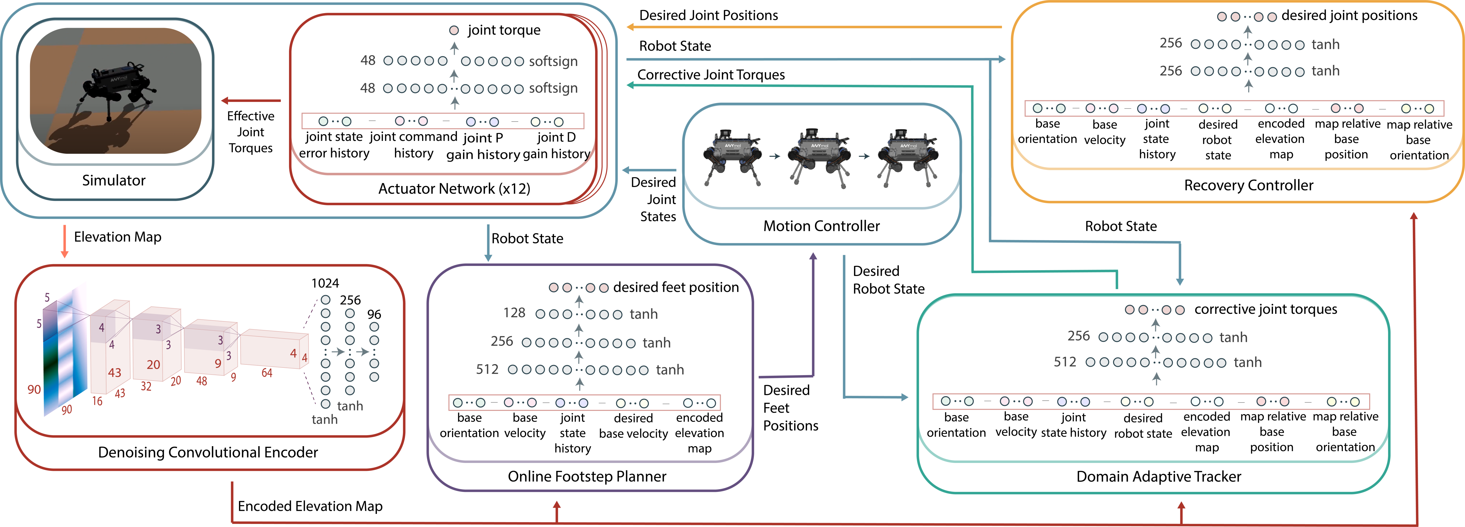
Figure 7: Overview of the approach used to train the RL policies as part of our framework. We introduce the denoising convolutional encoder to embed the elevation map into a lower-dimensional representation. This, along with the robot states and desired velocity commands becomes the observation space for each of the RL policies. Since we train the RL policies in simulation, we use an actuator network to approximately model the actuation dynamics of the real robot to make sim-to-real transfer feasible.

This section details upon the training, testing and deployment setups for each of the RL policies. We trained these policies using the RaiSim [46] physics simulator for its extremely fast contact dynamics computation. Moreover, RaiSim supports online reloading of heightmaps enabling the user to simulate terrains making it suitable for training terrain-aware RL policies. We defer the reader to our previous work [21] for a detailed analysis on the preference for RaiSim over other widely accessible simulation platforms. Figure 7 represents an overview of the training approach.

IV-A Footstep Planner

IV-A1 Terrain Generation

Similar to [29], we introduce a large set of terrains, 10k in our case where each terrain is represented as $\mathbf{T}\in\mathbb{R}^{1001\times 1001}$, into our simulation environment to obtain robust policies which can generalize to a wide domain of terrains. Our terrain generation procedure is similar to the one introduced in [47], and is further detailed in the Appendix.

IV-A2 Actuation Dynamics

As introduced in [19], we train an actuator network to model the actuation dynamics of the physical system to reduce the reality gap by emulating the impedance controller response as observed on the real robot. However, unlike in the case of [19, 21] where the actuators were modeled only for joint position targets with a predefined set of PD gains given by

$$\tau_{j}=\mathbf{j}_{G}(\mathrm{q}_{j}^{\ast},\mathrm{q}_{j},\mathrm{\dot{q}}_{j})\ ,$$ (23)

in this work, we trained the actuator network using supervised learning to obtain the effective actuation torques

$$\tau_{j}=\mathbf{j}_{R}(\mathrm{q}_{j}^{\ast},\mathrm{q}_{j},\mathrm{\dot{q}}_{j}^{\ast},\mathrm{\dot{q}}_{j},\tau_{j_{FF}},K_{p},K_{d})\ .$$ (24)

Since the motion controller utilizes different set of PD gains for joints of legs with foot in close, open and contact-uncertainty states, we further include the PD gains as an input to the approximated actuator model. Note that, even for the same contact states, the actuators located on the joints of the same limb can have different PD gains. The actuator network thus maps the input ${j}_{s}\in\mathbb{R}^{21}$ to an approximation of the joint torque, $\tau_{j}\in\mathbb{R}$, observed on the physical system. The network architecture and training details are provided in the Appendix.

IV-A3 Velocity command generation

In order to reduce computational overhead, our terrain generation tool does not include collision detection between objects. As a result, these terrains contain overlapping objects. In some cases, the terrains also have significant deviations in height in small regions which cannot be traversed due to the limited size of the robots. In this regard, we generate velocity commands with the assumption that the robot tracks the velocity commands perfectly. We then check for height deviations in the terrain for the next $400\text{\,}\mathrm{ms}$ along the robot’s expected trajectory. In case the height deviation exceeds the threshold of $0.4\text{\,}\mathrm{m}$, we generate new velocity commands until the height deviation along the expected trajectory remains less than the threshold. This height deviation test is performed every $100\text{\,}\mathrm{ms}$. The described velocity command generation approach significantly helps boost the performance of the footstep planning and domain adaptive tracking policies during training. Without introducing a strategic velocity command generator, we observed that our policies failed to converge, often resulting in reward collapse.

IV-A4 Domain randomization

Our footstep planner is trained to adapt to the behavior of the motion controller which significantly depends on the dynamic properties of the system. In order to achieve a locomotion behavior robust to change in system properties, such as added mass, we further utilize domain randomization strategies in addition to terrain randomization. These are shown in Table V. Note that the sampling distributions presented in Table V relate to the limits which the motion controller is robust to. We observed that increasing the range of the distributions caused motion tracking failure. In this regard, we perform two training sessions for the footstep planner. Session 1 employs the distributions presented in Table V, while Session 2 utilizes the domain adaptive tracker to enhance the robustness of the motion controller and therefore employs the distributions presented in Table VI. Furthermore, since the perception sensors present on the real robot cannot be used to perceive the elevation along regions occluded by an obstacle, we apply blurring filter to the elevation map, as shown in eq. 10, to emulate interpolation around unobservable terrain features.

We also apply external perturbations along $\mathbf{e}^{B}_{x}$ and $\mathbf{e}^{B}_{y}$. However, since the motion controller is not robust to perturbations of high magnitude, we sample the external forces from a normal distribution $\mathcal{N}(0,10)\,$$\mathrm{N}$ clipped between $[-30,30]\,$$\mathrm{N}$ for a duration in the range $[1,4]\,$$\mathrm{s}$. We also perform gait randomization, where we select the trot gait with a probability of 0.7, crawl with a probability of 0.2, and amble & pace with a probability of 0.05 each.

TABLE V: Domain randomization properties utilized in Session 1 for training the footstep planning policy.

Property	Sampling Distribution
Gravity, $g=$9.81\text{\,}\mathrm{m}\text{\,}{\mathrm{s}}^{-2}$$	$\mathcal{U}(0.96g,1.04g)$
Actuation Torque Scaling	$\mathcal{U}(0.9,1.1)$
Robot Link Mass Scaling	$\mathcal{U}(0.93,1.07)$
Robot Link Length Scaling	$\mathcal{U}(0.97,1.05)$

IV-A5 Reinforcement Learning

For Session 1, we employ an interactive direct policy learning approach to perform guided updates of our footstep planning policy, $\pi_{\theta_{f}}$, in order to increase sample efficiency during RL policy optimization. We initialize policy parameters, $\theta_{f}$, using Xavier initialization [48]. We consider a fixed-length episode of 1024 desired feet position samples, implying 1024 gait strides are executed in each episode. During training, we also perform locomotion over flat terrain. In this case, we use the motion controller to track the feet position generated by the policy and store it in a buffer $\mathcal{D}$. Additionally, we generate the desired feet position using the foothold optimizer of the Dynamic Gaits motion controller for the same robot state, $\mathbf{s}_{f}$, and add it to $\mathcal{D}$. After desired number of episodes used for locomotion over flat ground, we perform back-propagation through the footstep planning policy using the mean-squared error loss between the predicted and the expert samples. For uneven terrain, we utilize SAC to perform policy exploration so as to learn to generate feet position that avoid edges and slopes while ensuring the stability of the robot. We alternate between policy optimization through exploration and the interactive guided policy learning during training. The ratio of episodes used to perform guided learning to the number of episodes used to perform policy exploration is reduced as training progresses. We refer to this approach as interactive guided policy optimization (IGPO). Algorithm 1 describes the IGPO approach used for training the footstep planning policy. It is important to note that since we use a curriculum based reward transition given by the factor $d_{f}$ as shown in eq. 16 and eq. 17, we continuously push new state transition tuples to the SAC replay buffer while discarding the older samples to ensure that the action-value function approximations utilized in SAC remain relevant to the latest objective weighted by $d_{f}$. Moreover, while performing guided learning, we set the target value of the state-dependent stochasticity based on $\sigma_{\theta_{f}}(\mathbf{s}_{f})$ to zero.

1:Input: $\lambda_{d}$, $n_{eps}$, $l_{eps}$, $H$

2:Initialize $\mathcal{D}=\{\}$, $\alpha=1$

3:for $k=0,1,2\dots H$ do

4:     $\theta_{f},\mathcal{D}=\textsc{GuidedLearning}(\theta_{f},\mathcal{D},\alpha n_{eps},l_{eps})$

5:     $\theta_{f}=\textsc{PolicyOptimization}(\theta_{f},\left(1-\alpha\right)n_{eps},l_{eps})$

6:     $\alpha=\text{{e}}^{\lambda_{d}t}$

7:end for

8:function GuidedLearning($\theta_{f}$, $\mathcal{D}$, $n_{eps}$, $l_{eps}$)

9:     for $i=0$ to $n_{eps}-1$ do

10:         for $t=0$ to $l_{eps}-1$ do

11:              Sample $a\sim\pi_{\theta_{f}}\left(a|s\right)$

12:              Generate $a^{\ast}$ using DynamicGaits(s)

13:              $\mathcal{D}=\mathcal{D}\cup\left\{\left(s,a,a^{\ast}\right)\right\}$

14:              $s,r=\textsc{RLEnvironmentStep}(a)$

15:         end for

16:         Sample batch of $\{(s,a_{j},a_{j}^{\ast})\}$ from $\mathcal{D}$

17:         Update $\theta_{f}$ by minimizing $\sum_{j}{||a_{j}-a_{j}^{\ast}||^{2}}$

18:     end for

19:     return $\theta_{f}$, $\mathcal{D}$

20:end function

21:function PolicyOptimization($\theta_{f}$, $n_{eps}$, $l_{eps}$)

22:     for $i=0$ to $n_{eps}-1$ do

23:         $\tau=\{\}$

24:         for $t=0$ to $l_{eps}-1$ do

25:              Sample $a\sim\pi_{\theta_{f}}\left(a|s\right)$

26:              $s,r=\textsc{RLEnvironmentStep}(a)$

27:              $\tau=\tau\cup\left(s,a,r\right)$

28:         end for

29:         Update $\theta_{f}$ using SAC

30:     end for

31:     return $\theta_{f}$

32:end function

Algorithm 1 Interactive Guided Policy Optimization

As training progresses, we increase the complexity of the RL environment by scaling the maximum terrain elevation. As introduced in Section IV-A1, we represent the elements of $\mathbf{T}$ in the range of $[0,h_{max}]$ where $h_{max}=$2\text{\,}\mathrm{m}$$. During training, we scale $h_{max}$ using $d_{hf}$ which is updated by the rule $d_{{hf}_{k+1}}\leftarrow{}d_{{hf}_{k}}^{0.9992}$ where $k$ refers to the policy iterations and $d_{hf_{0}}=0.01$.

For Session 2, we do not perform guided learning and only utilize SAC to make footstep planning more robust to the changes in modeled system dynamics. We also set each of the curriculum factors to one. This additional training allows us to utilize the same footstep planner trained with ANYmal B for deployment on ANYmal C. The training hyperparameters and policy convergence iterations are provided in the Appendix.

IV-A6 Testing

For the purpose of evaluation, we utilize the stochastic policy in a deterministic manner. Therefore, we consider the $\mu_{\theta_{f}}(\mathbf{s}_{f})$ as the desired action, ${}_{H}r^{\ast}_{H{F_{x}y}}$, and discard $\sigma_{\theta_{f}}(\mathbf{s}_{f})$. We detail the test results in Section V-A.

IV-A7 Deployment

The observations utilized for the footstep planner are accessible on the physical robots. During deployment on the real robots, we observe a computational delay of approximately $35\text{\,}\mathrm{ms}$ during elevation map extraction and encoding. The elevation map processing is therefore executed in a parallel thread while the motion tracking controller runs in the main thread at $400\text{\,}\mathrm{Hz}$. The robot maintains the previous desired footholds while the forward pass through the elevation map encoder and the footstep planning policy is performed, after which, the new motion plans for the updated footholds are generated and tracked. This methodology remains consistent for both ANYmal B and C. A forward pass through the FP policy network requires approximately $195\text{\,}\mathrm{\SIUnitSymbolMicro s}$ on both the robots.

IV-B Domain Adaptive Tracker

We utilize the terrain generator, actuator network and velocity command generator introduced in Section IV-A for training the DAT policy. In addition, we use the footstep planning policy obtained after training Session 1 to train our domain adaptive tracking policy.

IV-B1 Domain Randomization

The randomization parameters and the corresponding sampling distributions representing the limits are provided in Table VI. During training of the DAT policy, the parameter randomization is approached using a curriculum learning setup where initial limits of the distributions are set to 1. The lower and upper limits are then linearly expanded after every policy iteration, $k$, based on the rule $l_{l,k}=max(\frac{k}{2000}(l_{min}-1)+1,l_{min})$ and $l_{u,k}=min(\frac{k}{2000}(l_{max}-1)+1,l_{max})$ respectively where the $l_{min}$ and $l_{max}$ are the lower and upper limits presented in Table VI. We also introduce external perturbations and gait randomization as done for the footstep planner.

TABLE VI: Domain randomization properties utilized for training the domain adaptive tracking policy. Here $\tau_{j}^{\ast}$ is the expected torque output of the impedance controller.

Property	Sampling Distribution
Gravity, $g=$9.81\text{\,}\mathrm{m}\text{\,}{\mathrm{s}}^{-2}$$	$\mathcal{U}(0.96g,1.04g)$
Actuation Torque Scaling	$\mathcal{U}(0.85,1.15)$
Robot Link Mass Scaling	$\mathcal{U}(0.9,1.10)$
Robot Link Length Scaling	$\mathcal{U}(0.85,1.15)$
Actuation Damping Gain $G$ such that $\tau_{j,t}=G\tau_{j,t}^{\ast}+(1-G)\tau_{j,t-1}$	$\mathcal{U}(0.8,1)$

IV-B2 Reinforcement Learning

We employ TD3 for training the DAT policy allowing us to perform constrained exploration. We observed that the stochasticity associated with policies trained using SAC and PPO required exhaustive hyperparameter tuning. Without significant tuning, the exploration resulted in introduction of large corrective torques. This caused the whole-body controller to significantly drift from the generated motion plans causing aggressive recovery and eventual failure. This inhibited learning since the corrective torques mostly resulted in episode termination. We therefore used TD3 to initially perform constrained exploration using uncorrelated Gaussian sampling. During training, we scale the standard deviation of the standard Gaussian distribution according to the rule $d_{a,k+1}\leftarrow d_{a,k}^{0.9994}$ where $k$ refers to the elapsed policy iterations and the initial scaling $d_{a,0}=0.01$. Additionally, we scale $\delta\tau_{j}$ by a factor of $40$ before adding it to the feed-forward torque generated by the whole-body controller.

As in the case of training the footstep planner, we use the same curriculum approach of scaling the maximum terrain elevation. We used the standard RLlib TD3 implementation for reinforcement learning. The hyperparameters are provided in the Appendix.

IV-B3 Testing

Since we obtain a deterministic policy, we do not perform any modifications to the neural network and directly employ it as a function mapping state to action. The test results are presented in Section V-B.

IV-B4 Deployment

The DAT is executed along with the whole-body controller in the main control loop at $400\text{\,}\mathrm{Hz}$. The generated corrective torques are then added to the output of the whole-body controller, after which the desired joint states are forwarded to the actuator. The DAT remains active when the recovery controller is deactivated. A forward pass through the DAT policy network requires approximately $66\text{\,}\mathrm{\SIUnitSymbolMicro s}$.

IV-C Recovery Controller

Our recovery controller training setup is directly built on top of our previous work [21]. However, unlike in the case of our previous work, we do not employ a guided policy optimization strategy, since the guided learning focused on velocity command tracking as opposed to recovery control, and instead utilize the training approach presented in [19] performing reinforcement learning using PPO.

For training the RC policy, we employ the terrain generator introduced in Section IV-A1. Since we perform joint position control with the recovery policy, we also use the actuator network to model the actuation dynamics for fixed $K_{p}=50$ and $K_{d}=0.1$ with zero velocity target. This is described in eq. 23. We defer the reader to the original work [19] for detailed description of the joint position target actuator network.

IV-C1 Domain Randomization

We use the same randomization strategy, including curriculum learning, as used for DAT for training the recovery controller.

IV-C2 Reinforcement Learning

Since our objective is to learn a recovery controller which can stabilize to perturbations in addition to performing state recovery, we introduce external perturbations in our training environment. However, in order to encompass a wide possibility of robot states when the recovery controller is activated, we initially train the RC policy to track reference velocity commands. We then transition from this objective to that of recovery control. For this, we initially learn to locomote over flat ground after which we introduce larger external perturbations while also scaling up the terrain elevation. The approach is detailed in Algorithm 2.

1:Input: $n_{eps}$, $l_{eps}$, $H$

2:Initialize $e_{max}=1e-4$, $f_{max}=0.01$, $t_{f_{max}}=0.01$, $t_{f}=0$, $t_{a}=0$

3:for $k=0,1,2\dots H$ do

4:     for $i=0$ to $n_{eps}-1$ do

5:         $t_{vel},s=\textsc{RLEnvironmentReset}(e_{max})$

6:         for $t=0$ to $l_{eps}-1$ do

7:              if $t>=t_{vel}$ then

8:                  Generate new velocity command

9:                  Sample $t_{vel}\sim\mathcal{U}(1,3)$

10:              end if

11:              Sample action $a\sim\pi_{\theta_{r}}\left(a|s\right)$

12:              if $t>=t_{a}$ and $t<t_{a}+t_{f}$ then

13:                  Apply external force $f$

14:              else if $t>t_{a}+t_{f}$ then

15:                  Sample external force, $f\sim\mathcal{N}(0,45f_{max})$

16:                  Sample $t_{a}\sim\mathcal{U}(t,t+2)$ and $t_{f}\sim\mathcal{U}(0,4t_{f_{max}})$

17:              end if

18:              $s,r=\textsc{RLEnvironmentStep}(a)$

19:              if $s$ is a terminal state then

20:                  $t_{vel},s=\textsc{RLEnvironmentReset}(e_{max})$

21:              end if

22:         end for

23:     end for

24:     Update $\pi_{\theta_{r}}$ using PPO

25:     $e_{max}\leftarrow e_{max}^{0.9996}$, $f_{max}\leftarrow f_{max}^{0.9984}$, $t_{f_{max}}\leftarrow t_{f_{max}}^{0.997}$

26:end for

27:function RLEnvironmentReset($e_{max}$)

28:     Sample terrain and scale elevation by $e_{max}$

29:     Randomize robot pose

30:     Randomize $\mathrm{q}_{j}$ where $max(|\mathrm{q}_{j}-\mathrm{q}_{j}^{n}|)<0.3$

31:     Randomize $\dot{\mathrm{q}}_{j}$ where $max(|\dot{\mathrm{q}}_{j}|)<1.0$

32:     Update state $s$ and set $t_{vel}=0$

33:     return $t_{vel}$, $s$

34:end function

Algorithm 2 Recovery Control Training Objective Transition

IV-C3 Testing

As in the case of FP, we utilize the stochastic policy in a deterministic manner. In this regard, the action $\mathbf{a}_{r}=\mu_{\theta_{r}}(\mathbf{s}_{r})$. The desired joint positions, $\mathrm{q}_{j}^{\ast}=\mathbf{a}_{r}$ are then forwarded to the actuator to generate the effective actuation torques. The results are presented in Section V-C.

IV-C4 Deployment

We query the robot state at each control step executed at $400\text{\,}\mathrm{Hz}$ to activate RC according to the limits described in Section III-E. When active, RC is run in the main control loop to generate the desired joint positions. While the RC remains active, the footstep planner, motion controller and domain adaptive tracker are deactivated. A forward pass through the RC policy network requires approximately $42\text{\,}\mathrm{\SIUnitSymbolMicro s}$.

V Results and Discussion

This section details the results obtained for each of the RL policies introduced in our framework. Note that, unless otherwise stated, the results presented here relate to the ANYmal B quadruped.

V-A Footstep Planning

We evaluate the footstep planning policy, obtained after the 2 training sessions, by measuring its success rate when traversing different terrains. We set up our simulation platform to perform 1000 runs for each of the 3 footstep planners navigating using 2 different gaits - trot and crawl. The 3 planners are our RL footstep planner, a baseline perceptive planner and a baseline blind planner. In the case of the baseline planners, we use the original foothold optimizer of dynamic gaits to generate $r_{F}^{d}$ for tracking the desired base velocity commands. We further modify $r_{F_{z}}^{d}$ by extracting the terrain elevation at the touch-down location directly from $\mathbf{M}_{H}$ (including for the blind controller). For the case of perceptive controller, we additionally adjust $r_{F_{xy}}^{d}$ up to a radial deviation of $0.05\text{\,}\mathrm{m}$ so as to minimize the cost $\mathbf{C}_{\mathbf{M}}(\hat{r}_{F_{xy},i})+2.5\|{\hat{r}_{F_{xy},i}-r^{n}_{F_{xy},i}}\|^{2}$ for each of the feet. For this optimization, we compute the cost by sampling $\hat{r}_{F_{xy},i}$ along the polar radial coordinate with a resolution of $0.005\text{\,}\mathrm{m}$ and a polar angular resolution of $\pi/18\;$\mathrm{rad}$$. We test the performance over 1000 different terrains of varying dimensions for each of the 4 object types - stairs, bricks, wave and unstructured ground as shown in Fig. 8. Each of these objects are located at the center of a $5\times 5\;$${\mathrm{m}}^{2}$ terrain, with the length of the object, along the direction of the robot’s frontal axis, varying between $2.0\text{\,}\mathrm{m}$ to $3.6\text{\,}\mathrm{m}$. We consider the following terrain properties.

1. The amplitude for the unstructured terrain is varied between $[0.0125,0.025]\,$$\mathrm{m}$.

2. For stairs, the number of steps range between $[3,8]$. The maximum terrain elevation is varied between $[0.25,0.8]\,$$\mathrm{m}$ using clipped normal distribution, $\mathcal{N}(0.3,0.1)\,$$\mathrm{m}$.

3. The wave terrain is generated using a sine function along its length with an amplitude range of $[0.05,0.1]\,$$\mathrm{m}$. The period of the sine function ranges between $\pi/2$ to $\pi$.

4. For brick terrain, the bricks are made of deformed $10\times 10$${\mathrm{cm}}^{2}$ patches with extrusions $\{-h,0,h\}$ where $h\in[0.02,0.05]\,$\mathrm{m}$$.

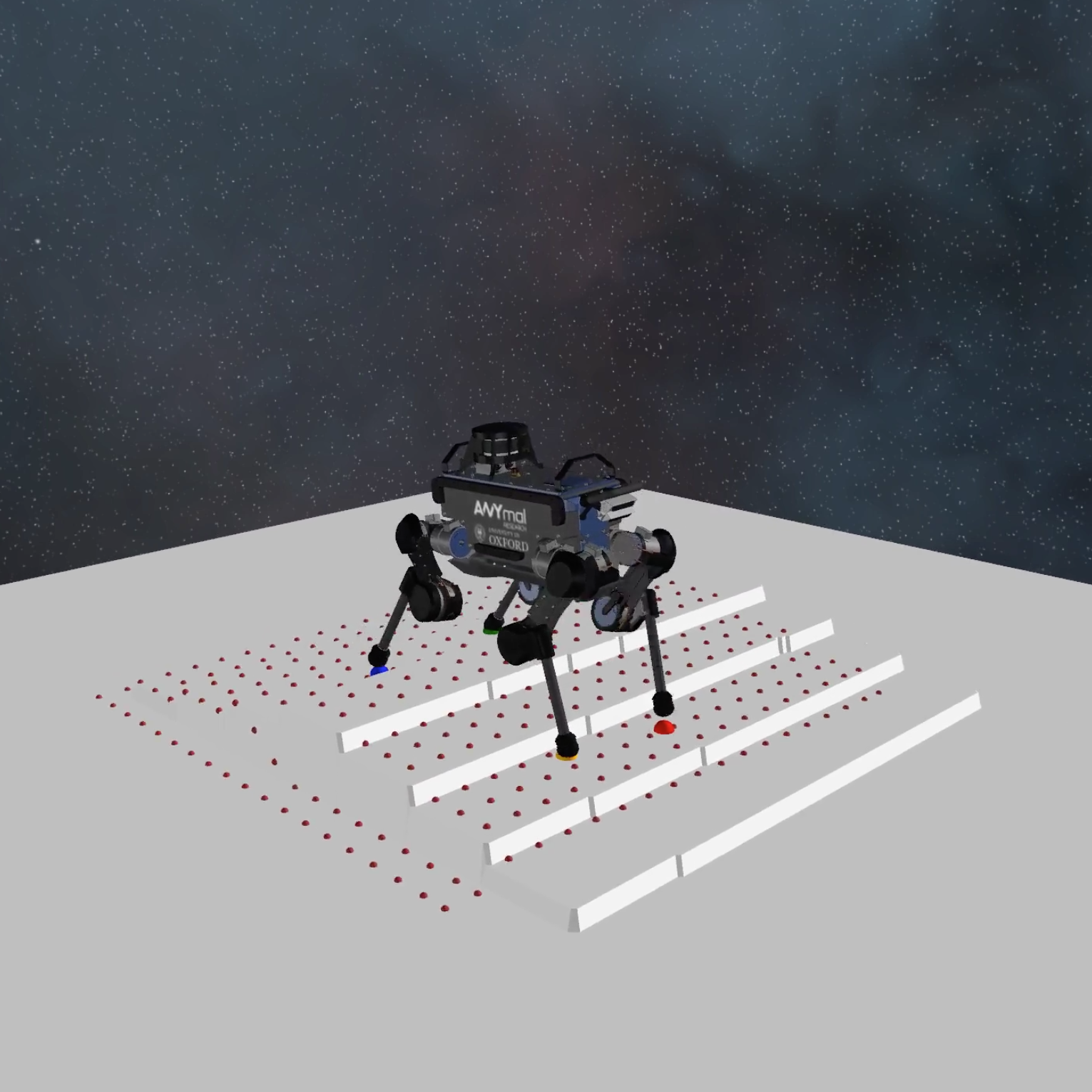
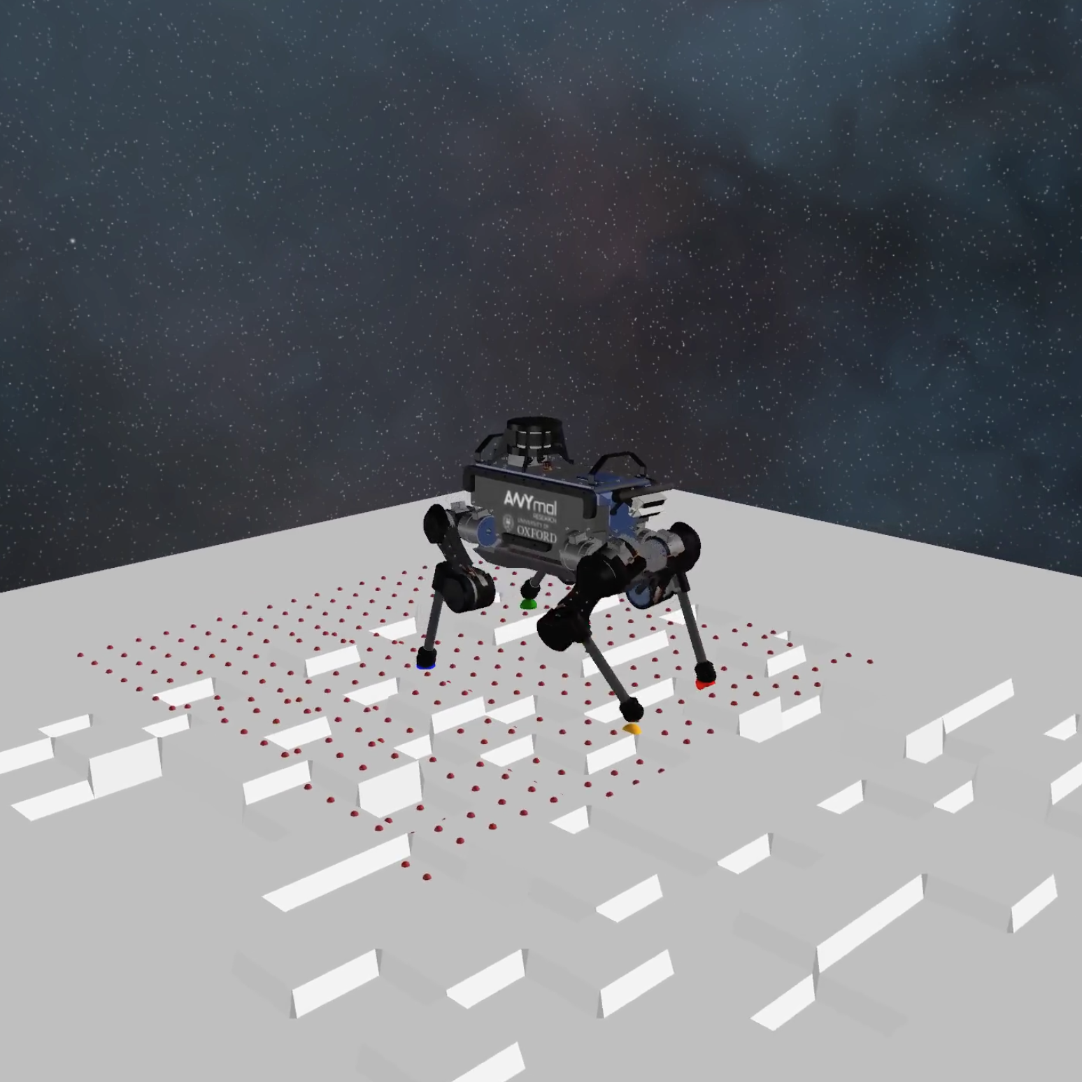
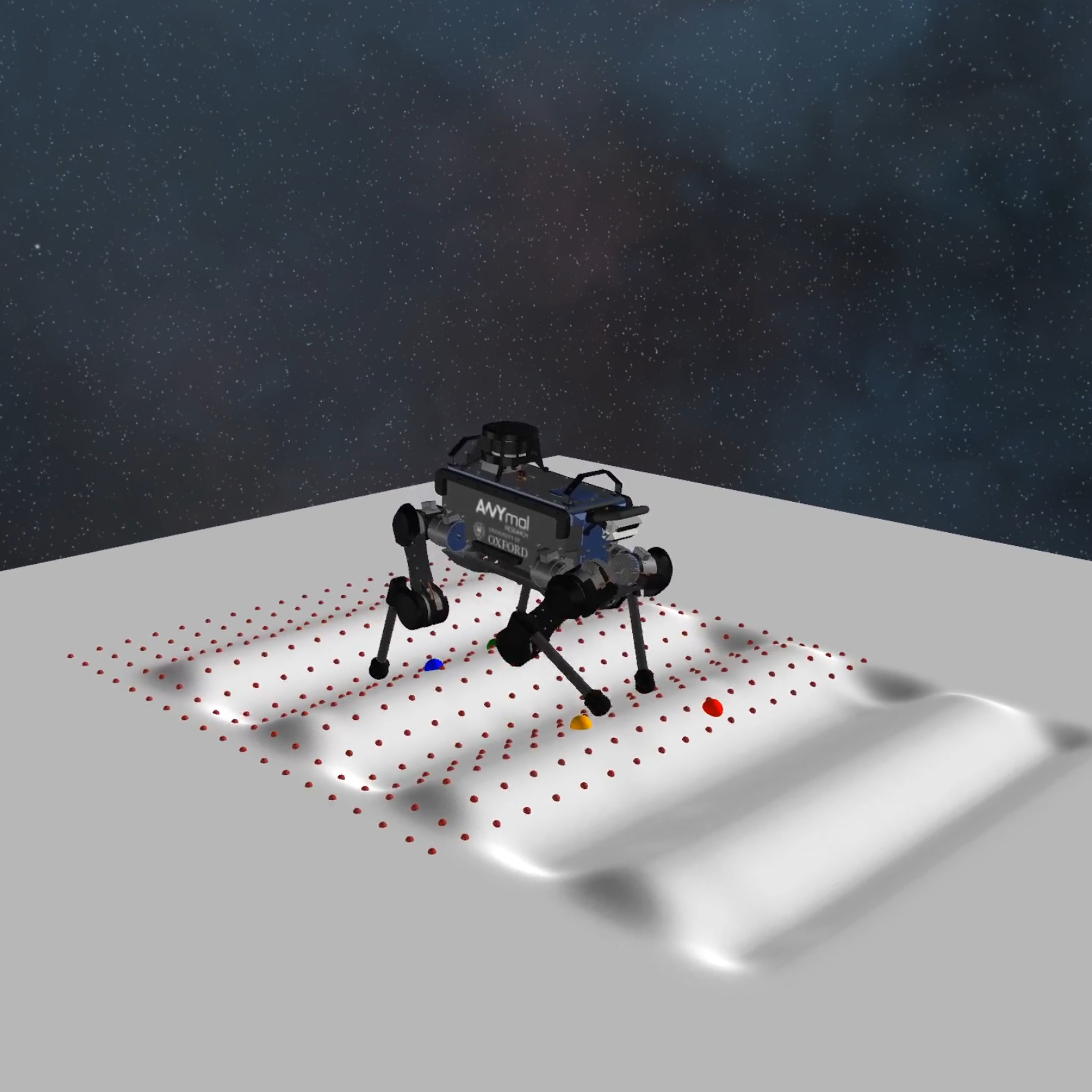
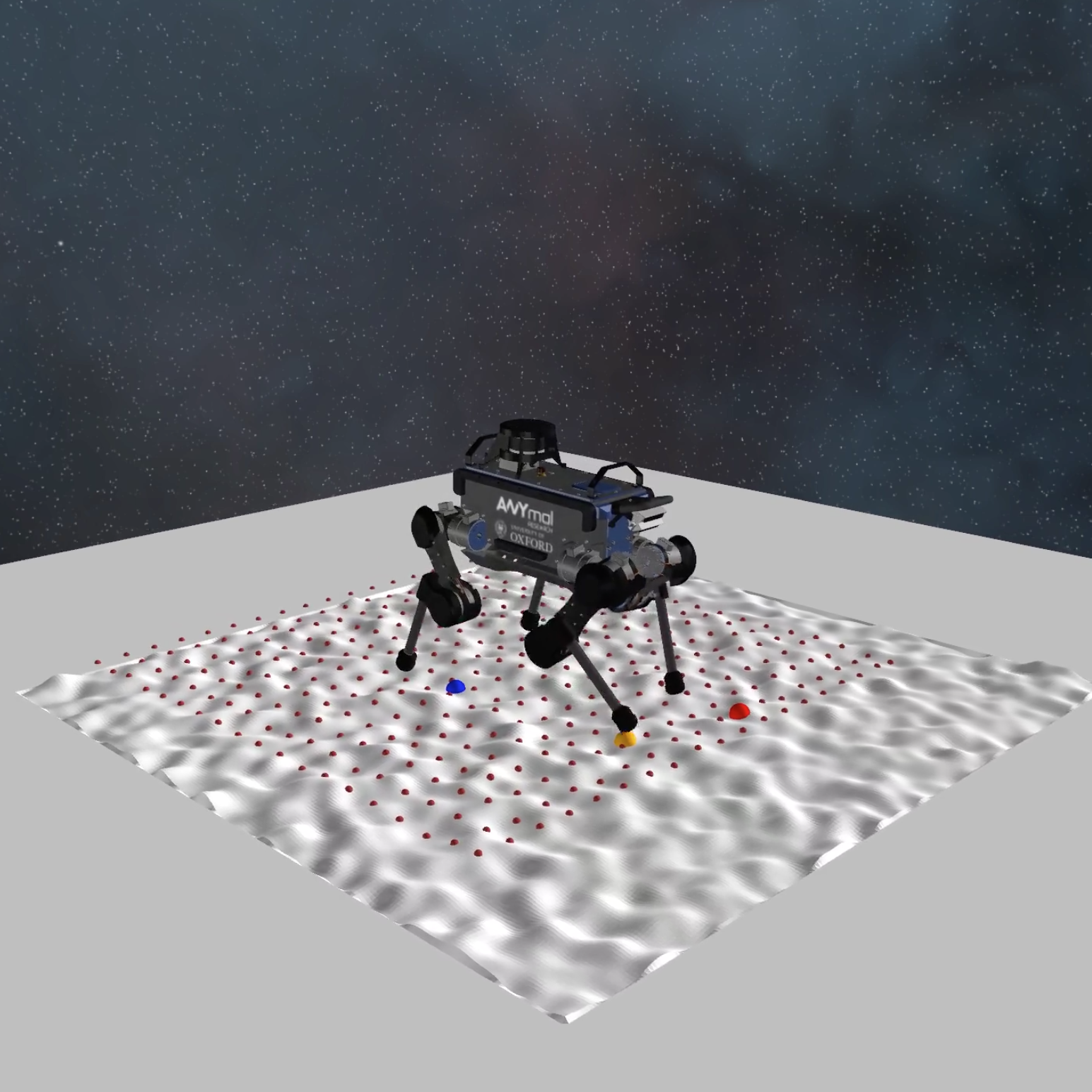
Figure 8: (Top) the stairs (left) and brick (right) terrains. (Bottom) the wave (left) and unstructured (right) terrains.

The results obtained for traversal over these terrains are presented in Movie S1.

For each run, we set the robot at the origin and generate a forward velocity command of $0.3\text{\,}\mathrm{m}\mathrm{/}\mathrm{s}$. We denote the run as a success if the robot traverses a distance of $4\text{\,}\mathrm{m}$, and regard it as a failure if any of the FP termination criteria is observed. The success rates obtained for each of the experiments are represented in Table VII. Figure 9 presents the success rate for traversing each terrain for each of the tested controllers with two gaits.

TABLE VII: Success rates of policies measured for locomotion over different terrains generated for 1000 runs each.

	Crawl			Trot
	Blind	Perceptive	RL Policy	Blind	Perceptive	RL Policy
Unstructured	99.6	99.4	99.9	99.7	99.6	99.6
Stairs	77.0	92.5	93.6	72.2	92.3	92.7
Wave	58.1	83.6	94.4	55.7	81.5	93.0
Bricks	52.1	71.5	88.2	51.1	70.9	85.3

The RL footstep planner was observed to exhibit preference for wider stance. This directly corresponds to a higher stability margin, a term introduced in the reward function during training. We measured ${}_{H}r_{HF}$ after every gait stride. For traversal over stairs, the absolute mean foot position in frame $H$ was $0.35\text{\,}\mathrm{m}$ and $0.20\text{\,}\mathrm{m}$ along its $x$ and $y$ axes, similar to the expected nominal stance value of $0.35\text{\,}\mathrm{m}$ and $0.20\text{\,}\mathrm{m}$. However, in the case of unstructured terrain, we computed the mean feet position to be $(0.34,0.23)$$\mathrm{m}$, $(0.35,0.21)$$\mathrm{m}$ for the wave terrain, and $(0.34,0.22)$$\mathrm{m}$ for the bricks terrain.

Figure. 9(e) represents the success rate as a function of step height and depth evaluated using kernel density estimation (KDE).

The extrusions in the brick terrains often caused leg blockages. This was prominent for the blind planner. The ability of the perceptive planner to minimize distance from the edges in the terrain significantly reduced the problem with leg blockage. However, the difference in the feet height resulted in the robot toppling over in most cases. With the RL planner, we observed a wide stance and preference for foot placement along regions which minimized the deviation in feet height. For the case of the blind planner, we computed a mean deviation between the maximum and minimum foot height to be $0.074\text{\,}\mathrm{m}$. For the perceptive planner the mean height deviation was $0.083\text{\,}\mathrm{m}$, and $0.057\text{\,}\mathrm{m}$ with the RL planner. Figure 9(f) illustrates the success rate computed for different brick heights. In this case, the brick height only corresponds to the extrusion of the terrain implying that the maximum deviation in feet height is twice the height of the bricks. We observed that the RL planner fails to traverse brick terrains with maximum elevation of higher than $0.12\text{\,}\mathrm{m}$ (corresponding to a maximum height deviation of $0.24\text{\,}\mathrm{m}$). This mainly occurs due to the limitations of the physical dimensions of the quadruped.

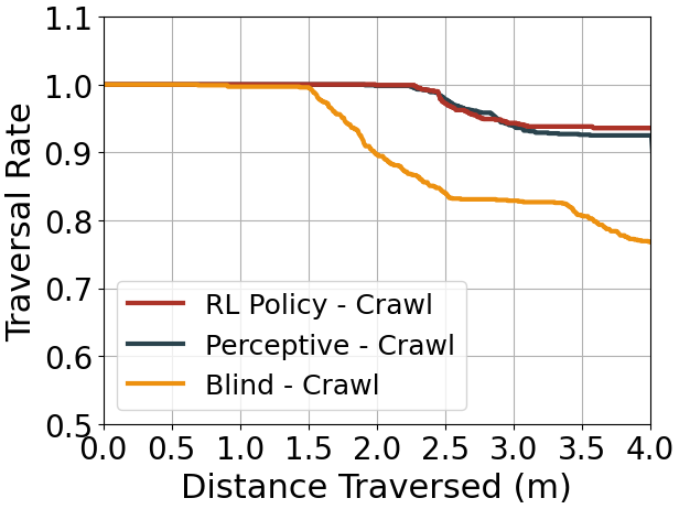
(a) Stairs

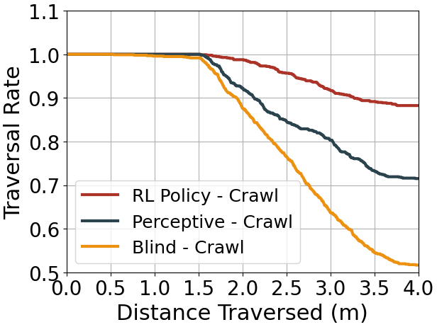
(b) Bricks

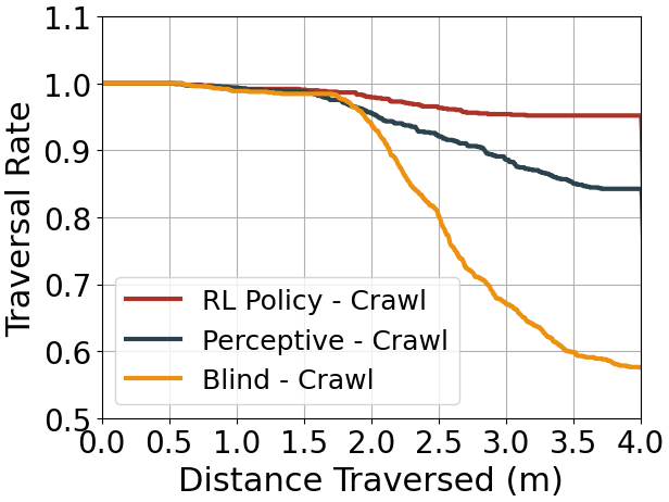
(c) Wave

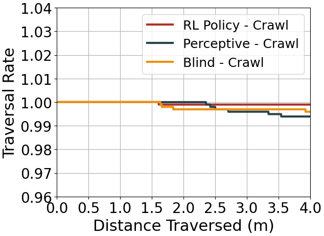
(d) Unstructured

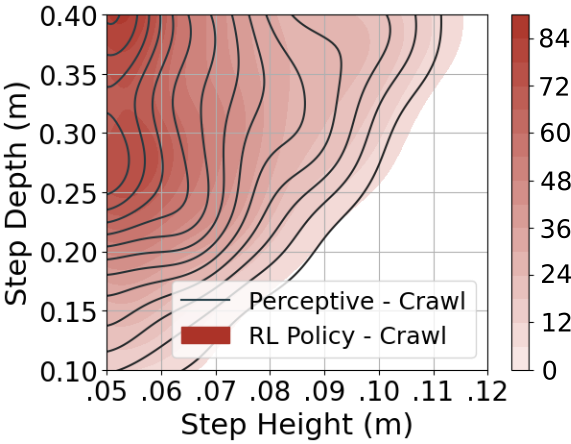
(e) Estimate of success rate for
traversal over stairs with varying
depth and height

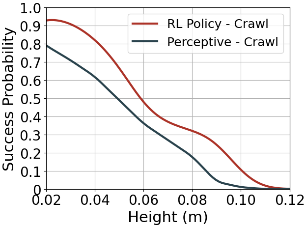
(f) Estimate of success rate for
terrains with varying brick height

Figure 9: (a-d) represent the traversal rate of each of the planning policies for the different types of terrains used for evaluation. This corresponds to the rate of success observed for the distance traversed. (e) is the plot representing the success rate for traversal over stairs with varying step height and depth. (f) represents the probability of success observed for brick terrain of varying brick heights.

We also compared the generalization capability of the footstep planner obtained after training Session 1 and Session 2. We performed the experiments discussed above using the ANYmal C quadruped, adapting the motion controller for the parameter description of ANYmal C. The corresponding success rates are presented in Table VIII. As expected, we observe a better ability to generalize to a different platform with the policy trained using significant domain randomization.

TABLE VIII: Success rates obtained for locomotion over different terrains using the ANYmal C quadruped comparing the RL footstep planner performance after training Session 1 and Session 2.

	Crawl		Trot
	Session 1	Session 2	Session 1	Session 2
Unstructured	99.9	99.9	99.4	99.5
Stairs	93.0	93.4	90.5	91.9
Wave	85.7	91.2	82.4	88.4
Bricks	76.3	85.8	71.6	82.2

V-B Domain Adaptive Tracking

In our experiments, the tracking error associated with the whole-body controller was negligible when the robot’s base mass, of $18.3546\text{\,}\mathrm{kg}$, was scaled in the range $\left[0.95,1.05\right]$.

However, when we decreased the mass by a factor below 0.94, or increased it beyond 1.06, the motion controller became unstable resulting in increased oscillations. This was caused due to the whole-body controller aggressively correcting for imprecise motion tracking. Introducing DAT helped stabilize whole-body motion tracking. We were able to scale the base mass in the range of $[0.84,1.17]$ without increasing the amplitude of the oscillations. Figure 10(a) illustrates the $\mathrm{p}_{CoM_{x}}$ tracking error observed before episode termination for different robot base masses. Here, the episode termination criteria include traversing a distance of $5\text{\,}\mathrm{m}$ or failure of whole-body control.

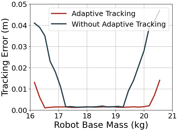
(a) ANYmal B

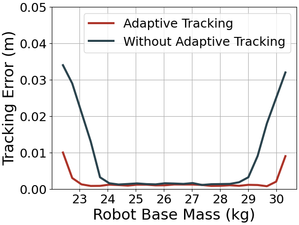
(b) ANYmal C

Figure 10: The absolute mean tracking error observed before termination for varying physical parameters of the robot comparing the effects of the domain adaptive tracking policy.

We also tested our domain adaptive tracking policy, without retraining, on the simulated model of the ANYmal C quadruped. Note that, while running experiments on the simulated ANYmal C, we increased the joint torque limit from $\pm 40\text{\,}\mathrm{N}\text{\,}\mathrm{m}$ for the case of ANYmal B to a limit of $\pm 80\text{\,}\mathrm{N}\text{\,}\mathrm{m}$. The tracking error measured for varying base mass of the ANYmal C quadruped is represented in Fig. 10(b). With an original base mass of $26.3732\text{\,}\mathrm{kg}$, the motion controller could track the forward velocity command of $0.3\text{\,}\mathrm{m}\mathrm{/}\mathrm{s}$ even when we scaled this mass in the range $\left[0.91,1.10\right]$. When we introduced the domain adaptive tracking policy, we were further able to extend this range to $\left[0.81,1.19\right]$.

We performed another test on the simulated ANYmal C robot. However, in this case, we used the parameter description of the ANYmal B quadruped. Therefore, the motion controller generated motion plans and control behavior for the ANYmal B quadruped even though the controller was used on ANYmal C. Note that, the domain adaptive policy was never trained using ANYmal C. Figure 11 represents the velocity tracking error observed in 1M simulation samples for randomly generated desired base velocity commands in the range of $[-0.3,0.3]$$\mathrm{m}\text{\,}{\mathrm{s}}^{-1}$ and $[-0.3,0.3]$$\mathrm{rad}\text{\,}{\mathrm{s}}^{-1}$ for the linear and angular velocities respectively. Note that, in this case of domain adaptive tracking, we did observe an oscillatory behavior in the limbs while tracking the base velocity commands. This was largely due to the whole-body controller outputting desired joint states which were then aggressively corrected by the domain adaptive tracking policy. Moreover, the domain adaptive tracker failed to stably track absolute velocity commands beyond $\pm 0.4$$\mathrm{m}\text{\,}{\mathrm{s}}^{-1}$ for heading velocity, $\pm 0.3$$\mathrm{m}\text{\,}{\mathrm{s}}^{-1}$ for lateral velocity, and $\pm 0.5$$\mathrm{rad}\text{\,}{\mathrm{s}}^{-1}$ for yaw rate.

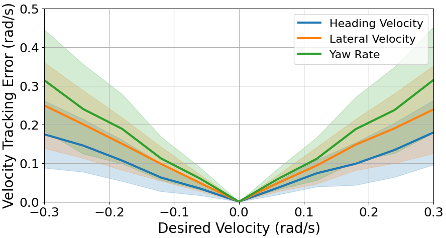
Figure 11: Velocity tracking error observed for the domain adaptive tracking policy when running the motion controller on ANYmal C with the description parameters of ANYmal B.

Figure 12 represents the mean and standard deviation of the absolute corrective joint torque generated by DAT to address ANYmal B base mass and link length scaling for locomotion on flat ground for a heading velocity command of $0.5\text{\,}\mathrm{m}\text{\,}{\mathrm{s}}^{-1}$.

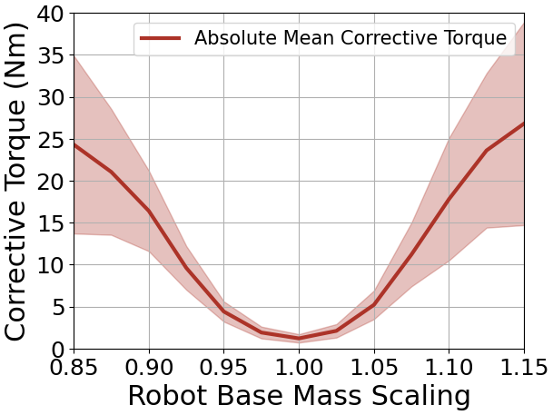
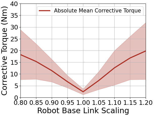
Figure 12: The absolute mean corrective torques generated by the DAT to minimize motion plan tracking errors for ANYmal B base mass (left) and link (right) scaling. The color bands represent one standard deviation.

We have also provided a set of examples employing the domain adaptive tracker in Movie S2.

V-C Recovery Controller

We tested the behavior of the RL recovery control policy and the motion controller for a range of external forces applied to the robot’s base along the heading and lateral axes for duration between $[0.5,2.5]\,$$\mathrm{s}$. The observations representing the KDE of the recovery rate as a function of the magnitude and duration of the external force for each of the controllers are as shown in Fig. 13. The color-bar labels represent the success probability of the robot to stabilize following external perturbations. We measure this for both ANYmal B and ANYmal C and observe that compared to the motion controller which can handle perturbations of up to approximately $100\text{\,}\mathrm{N}$ along the x-axis for the ANYmal B quadruped, the RL policy can handle external force of up to approximately $225\text{\,}\mathrm{N}$ and $400\text{\,}\mathrm{N}$ for ANYmal B and ANYmal C respectively. It is important to note that for the case of ANYmal C, we increased the position tracking gain to 60 compared to 45 for ANYmal B and also increased the joint torque limits to $\pm 80\text{\,}\mathrm{N}\text{\,}\mathrm{m}$ compared to $\pm 40\text{\,}\mathrm{N}\text{\,}\mathrm{m}$ for ANYmal B. The results obtained are also demonstrated in Movie S3.

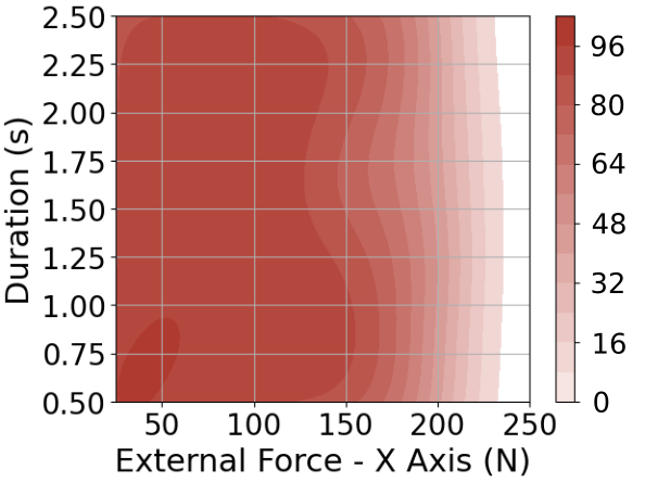
(a) RL recovery controller -
ANYmal B

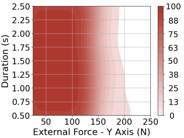
(b) RL recovery controller -
ANYmal B

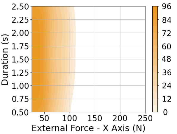
(c) model-based controller only

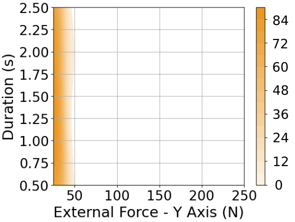
(d) model-based controller only

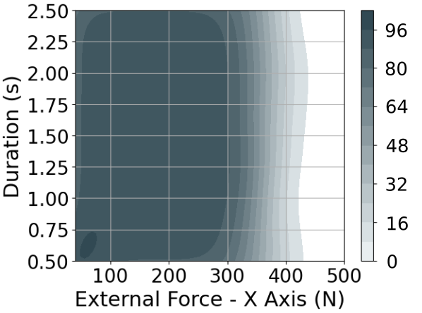
(e) RL recovery controller -
ANYmal C

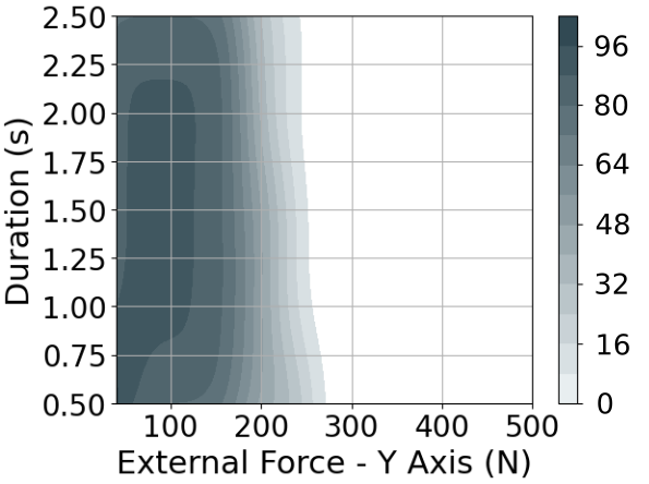
(f) RL recovery controller -
ANYmal C

Figure 13: Bivariate kernel density estimates representing the success probability of the control policies to stabilize upon external perturbations along the frontal (x) and the laeral (y) axes. Note that for (e-f) the x-axis scale of the plots is different.

V-D RLOC

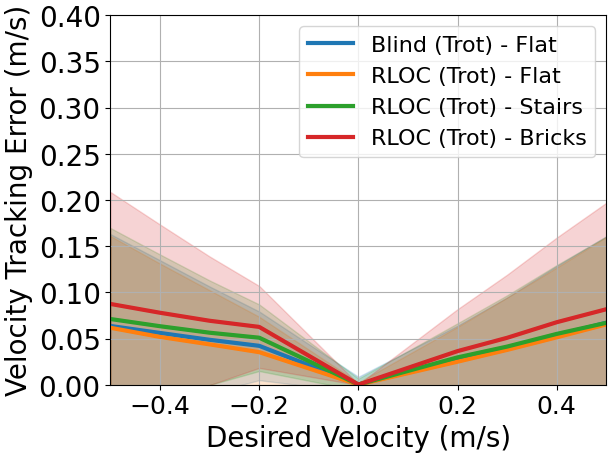
(a) Forward Velocity Tracking

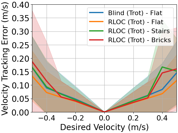
(b) Lateral Velocity Tracking

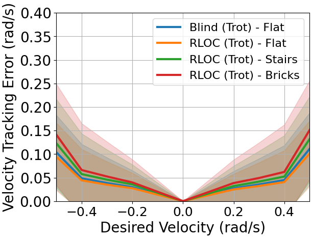
(c) Yaw Rate Tracking

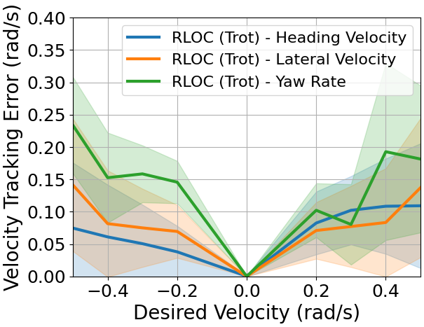
(d) Velocity Tracking - Gazebo

Figure 14: (a-c) represent the velocity tracking error measured for locomotion over even and uneven terrain for the ANYmal B quadruped tested in the RaiSim simulator. (d) represents the velocity tracking error on flat ground observed for the RLOC framework in the Gazebo simulator (with different actuation dynamics).

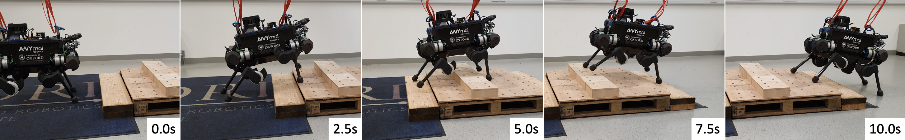
Figure 15: Snapshots of the ANYmal B quadruped walking over a staircase using our RLOC framework.

Figure 14 represents the tracking error observed for the RLOC framework for traversal over different types of terrains. The improved tracking performance over the motion controller was a direct result of introduction of DAT. Removing DAT resulted in a very similar performance as that of the motion controller.

The experimental setups for each of these terrains included the generation of a velocity command in the range of $[-0.5,0.5]$$\mathrm{m}\mathrm{/}\mathrm{s}$ for heading and lateral velocity tracking, and in the range of $[-0.5,0.5]$$\mathrm{rad}\mathrm{/}\mathrm{s}$ for desired yaw rate tracking. Each episode comprised tracking of a set velocity command for a duration of $5\text{\,}\mathrm{s}$. We performed 100 runs for each command.

In order to quantify the effects of the recovery control policy, we performed experiments using the bricks and wave terrains for the trotting gait as introduced for evaluation of the FP. This is further presented in Movie S3. Introduction of the recovery controller resulted in improved success rates. The results are summarized in Table IX.

TABLE IX: Improvement in success rate (SR) observed after introducing the recovery controller (RC) for traversal over bricks and wave terrains. The episodes here refer to the number of episodes (out of 1000) in which the RC was called. Moreover, the recovery rate (RR) represents the successful recovery performed using RC. The RR and SR are expressed as %.

	RC Calls	Episodes	RR	SR w/o RC	SR with RC
Bricks	184	131	62.5	85.3	90.2
Wave	39	22	71.8	93.0	94.8

We evaluated the velocity tracking performance of our framework in a slower but higher resolution Gazebo simulator [49], employing the ODE physics engine [50], as presented in Fig. 14(d). Figure 1 presents examples of the experiments performed on the real ANYmal B quadruped. The corresponding video clips are included in Movie 1. Figure 15 represents the snapshots of the robot ascending and descending a staircase. In our experiments with the real robot, we observed motion behavior similar to the behavior in RaiSim especially for tests on simpler terrains such as a staircase. In the case of bricks, however, the state-estimation drift, sensor noise and the fast but less accurate nearest-neighbor interpolation technique used to obtain the elevation map along occluded regions sometimes resulted in the elevation map being distorted especially along the edges, and also slightly shifted with respect to the robot. The distortion of the elevation map is illustrated in Fig. 4, Fig. 16 and Movie S4 which represent the real ANYmal B quadruped tested on a terrain comprising bricks, and the corresponding visualization of the robot state and the elevation map. This blurring and slight shifting of the elevation map caused the robot to step close to the edges especially in environments composed of a large number of small objects.

TABLE X: Success rate obtained for traversal over different terrains using the ANYmal C quadruped comparing the performance of RLOC with a baseline perceptive controller [34].

	Unstructured	Stairs	Wave	Bricks
RLOC (Trot)	99.6	93.0	91.2	89.3
Baseline	99.4	93.2	83.5	70.9

We compared the performance of RLOC on simulated ANYmal C with an open-sourced implementation of [34] as baseline. The success rates (for 1000 runs each) obtained for traversal over different terrains are provided in Table X. While the two control frameworks performed similarly for locomotion over unstructured and stairs terrain, the baseline controller was unable to stably traverse the brick terrain. This is mostly due to the significantly larger terrain elevation sampling resolution of $0.1\text{\,}\mathrm{m}$ utilized in [34] compared to $0.02\text{\,}\mathrm{m}$ as used in RLOC. Reducing the sampling resolution for the baseline is expected to require significant retuning of the training environment and the policy architecture. Although the baseline controller offered slightly better performance for traversing stairs, we observed that the controller was unable to reliably avoid edges while often staggering. In contrast, the motions exhibited by RLOC were a lot smoother. We suspect this behavioral comparison is also valid for [30]. This is attributed to the complex reward functions employed for training RLOC policies which encourage stable maneuvers (stability margin reward) while avoiding terrain edges (terrain cost map).

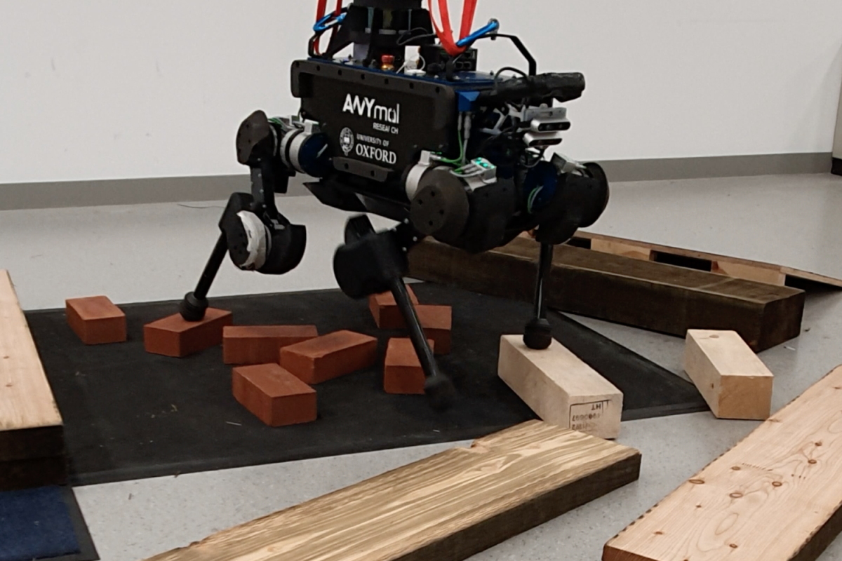
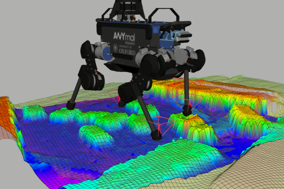
Figure 16: ANYmal B quadruped tested on a terrain comprising bricks (left); visualization of the corresponding robot state and elevation map (right).

We also transferred the RLOC framework to the real ANYmal C quadruped for both indoor and outdoor locomotion as shown in Fig. 2. We were able to locomote outdoors over grassy and muddy terrain, and slopes. We observed a similar behavior as in the case of ANYmal B, however, the ANYmal C offered an advantage of higher joint torque limits enabling us to ascend steeper slopes. For this transfer, the only changes included the robot parameter description for the motion controller and the impedance controller gains. The experiments performed with the real ANYmal B and ANYmal C are presented in Movie 1 and Movie S6.

We observed that ascending steep staircases where the ANYmal B base pitch exceeds $\pi/4\;$\mathrm{rad}$$ with respect to the horizontal frame results in failure to track heading velocity commands where the robot is unable to move forward. This is partially attributed to the joint torque limits while also resulting from the CoM motion planner that uses ZMP, implicitly assuming constant base height and attitude. For ANYmal C, we observe velocity command tracking failure beyond a pitch angle of approximately $\pi/3\;$\mathrm{rad}$$. This was the case for both simulated and real robot.

VI Conclusion and Future Work

We presented an approach which bridges the gap between policies trained using RL and controllers developed using model-based optimization methods. Our modular framework allowed us to greatly improve the success of traversal over complex terrains. For traversal over the bricks environment, as presented in Section V, we showed that our hybrid approach, RLOC, was able to increase the success rate from 71.5% (Table VII) to 90.2% (Table IX) in comparison to our baseline perceptive controller. We showed that we were able to traverse reliably (i.e. with a success rate of 90% or above over 4m) and with a dynamic gait (trot at an effective velocity of approximately 0.25$\mathrm{m}\text{\,}{\mathrm{s}}^{-1}$ on the real robot) over uneven terrain even though the model-based locomotion controller was primarily developed and tuned for quasi-flat terrains.

To address ascending steep stairs and slopes, in our future work we aim to learn a CoM and foot motion planner. Another direction for future work includes obtaining a hybrid long and short horizon planning policy to avoid obstacles and perform CoM and feet motion adaptations for traversal over extremely complex and non-stationary terrains.

Nomenclature

Notation	Definition
${}_{W}r_{WB}$ or $r_{B}$	translation of frame $B$ represented frame $W$
$\mathbf{R}_{WB}$ or $\mathbf{R}_{B}$	rotation matrix of $B$ represented in $W$
$\mathbf{e}_{z}^{W}$	$z$-axis of $W$
$\mathrm{q}_{j}$	joint positions
${}_{W}\mathrm{v}_{WB}$ or $\mathrm{v}_{B}$	linear velocity of $B$ measured and expressed in $W$
${}_{W}\mathrm{\omega}_{WB}$ or $\mathrm{\omega}_{B}$	angular velocity of $B$ measured and expressed in $W$
$\dot{\mathrm{q}}_{j}$	joint velocities
$\mathbf{R}_{B_{z}}$	$z$ decomposition of $\mathbf{R}_{B}$
$\tau_{j}$	joint torques
$\cdot^{\ast}$	desired quantity
$\Phi$	feet motion parameterization tuple
$r_{F}^{l}$, $r_{F}^{d}$, $r_{F}^{h}$	feet lift-off, touch-down and clearance positions
$\mathrm{c}_{F}$	feet contact state
$t_{F}^{l}$, $t_{F}^{d}$	feet lift-off and touch-down times
$\mathbf{M}_{H}$	robocentric terrain elevation represented in frame $H$
$\mathrm{Z}_{\mathbf{M}_{H}}$	latent embedding of $\mathbf{M}_{H}$
$\mathcal{C}$	2d convolution operator
$\mathbf{s}_{f}$, $\mathbf{a}_{f}$, $\mathbf{r}_{F}$	footstep planner state, action and reward
$\mathbf{s}_{d}$, $\mathbf{a}_{d}$, $\mathbf{r}_{D}$	domain adaptive tracker state, action and reward
$\mathbf{s}_{r}$, $\mathbf{a}_{r}$, $\mathbf{r}_{R}$	recovery controller state, action and reward
$\mathbf{c}^{\ast}$	desired velocity command
$\pi_{\theta_{f}},\pi_{\theta_{d}},\pi_{\theta_{r}}$	footstep planning, domain adaptive tracking and recovery control policies
$\mathcal{S}_{m}$	stability margin function
$\mathbf{C}_{\mathbf{M}}$	terrain cost map operator
$B_{\mathbf{M}_{H}}$	elevation map update frame

Appendix

VI-A Motion Controller

The dynamic gaits motion controller [31] generates the CoM motion plan by solving a nonlinear optimization problem using the sequential quadratic programming (SQP) approach [51] for a time horizon $t_{H}^{c}$ which corresponds to the periodicity of the active locomotion gait. The SQP optimization parameters correspond to the spline coefficients $\alpha=[{\alpha_{0}}^{T}\cdot\cdot\cdot{\alpha_{i}}^{T}\cdot\cdot\cdot{\alpha_{n_{s}}}^{T}]$ where $n_{s}$ is the number of different support polygons on the optimization horizon. This formulation, where the SQP also optimizes for ${\alpha_{i}^{z}}$ as opposed to assuming a fixed base height to ease on the computational complexity, enables us to adapt the dynamic gaits motion controller for locomotion over uneven terrain. For stability, dynamic gaits uses constraints on the ZMP. It also penalizes deviations from a path regularizer, which represents an approximated CoM motion plan for a duration of $t_{H}^{c}$, to limit the drift of the robot base w.r.t. the reference footholds which may occur due to external perturbations and continuous updates of the motion plan. The path regularizer, $\mathcal{T}_{R}^{c}$, is computed based on the estimated footprint center and the reference base velocity command, $\mathbf{c}^{\ast}$. We use a similar approach as presented in [31] to compute $\mathcal{T}_{R}^{c}$ and introduce the following adaptations in the CoM motion plan optimization problem: (1) the terrain plane is estimated by fitting a planar surface through the current and planned footholds as opposed to current and previous footholds (2) unlike dynamic gaits which sets the height of the path regularizer $\mathcal{T}_{R_{z}}^{c}$ at a fixed reference value $h_{ref}$ with respect to the control frame, we adapt this value such that:

$$\mathcal{T}_{R_{z}}^{c}=\mathbf{M}_{H}(\mathcal{T}_{R_{x}}^{c},\mathcal{T}_{R_{y}}^{c})+h_{ref}-0.125|\mathbf{R}_{C_{y}}|$$

where $\mathbf{R}_{C_{y}}$ is the angle of the terrain plane on the pitch axis of the robot. This modification allows us to increase the reachability of the feet on stairs and complex terrains.

The support polygons (used in the dynamic constraints of the optimization) are defined by separate modules, the foothold planner and contact scheduler.

The foothold planning module in dynamic gaits is set up as a quadratic programming (QP) problem to obtain the $x$ and $y$ components of the desired footholds ${r^{\ast}_{F_{xy}}}$. The nominal footholds expressed in the horizontal reference frame ${{}_{H}r^{n}_{HF_{xy}}}$ corresponds to the projections of the robot hip locations measured and expressed in the horizontal frame along the vertical axis ${\mathbf{e}_{z}^{H}}$. The cost function of the QP problem then includes, among others, a penalty term for deviations from the nominal foothold locations. The foothold optimizer gives us the desired feet touch down positions, ${r_{F}^{d}}^{\ast}$, where ${r^{d}_{F_{z}}}^{\ast}$ is extracted from the terrain plane estimate, for each swing phase.

The contact scheduler module, manages the feet contact-events for a full stride of an active gait while also supporting smooth gait transitions giving us the lift-off, $t_{F}^{l}$, and touch-down, $t_{F}^{d}$, timings for the feet swing and stance phases based on the assumption that $v_{F}^{l}$ and $v_{F}^{d}$ are zeros. This module also enables slowing down the execution of the gait in case a touch-down event is not detected at the expected time. The $\Phi_{o}$ and $\Phi_{c}$ thus obtained is used for generating motion plans for ${r_{F}^{d}}^{\ast}$. Moreover, dynamic gaits considers a fixed foot clearance position ${r_{F}^{h}}$ for $\Phi_{o}$.

In our RLOC framework, the foothold optimizer is replaced by the RL footstep planner which generates the desired feet touch-down positions, ${r_{F}^{FP}}$, for locomotion over uneven terrain. Additionally, ${r_{F,i}^{h}}$ for swing phase $\Phi_{o,i}$ of foot $i$ is now computed based on the maximum terrain elevation observed between the line, $l_{ld}^{\Phi}$, connecting $r_{F_{xy}}^{l}$ and ${r_{F_{xy}}^{FP}}$, given by

$$r_{{F_{z}},i}^{h}=\mathrm{max}(\mathbf{M}_{H}(X,Y))+0.05\,$\mathrm{m}$$$ (25)

where $\mathbf{M}_{H}$ is the elevation map expressed in the global reference frame, $X$ and $Y$ are the vectors containing the $x$ and $y$ coordinates of $l_{ld}^{\Phi}$ sampled at a resolution of $0.02\text{\,}\mathrm{m}$. The additional offset of $0.05\text{\,}\mathrm{m}$ to the foot clearance position is introduced to avoid collisions during inaccurate motion tracking. To limit uncertain behavior that may occur due to imprecise elevation map generation as a result of sensor noise and occlusions, $r^{h}_{F}$ is clipped to be less than $r^{l}_{F}+0.25\,$$\mathrm{m}$.

In contrast to dynamic gaits, which uses the estimate of the terrain plane to determine the orientation of the friction cone, we compute the terrain normal at each foot using the information from the elevation map. The normals are estimated using central finite difference at the feet positions. Since the information from the elevation map is not always reliable, we also add the following checks:

1. When $\mathrm{c}_{F,i}=1$, the foot height is close to the terrain elevation such that $|r^{d}_{{F}_{z},i}-\mathbf{M}_{H}(r^{d}_{{F_{xy},i}})|<\epsilon_{d}$ where $\epsilon_{d}=$0.04\text{\,}\mathrm{m}$$.

2. The terrain elevation within a deviation of $\pm$4\text{\,}\mathrm{cm}$$ centered at $r^{d}_{F_{xy},i}$ is planar.

3. The estimated terrain normal at foot $i$, $\mathbf{e}_{z}^{T_{i}}$, stays in realistic bounds, i.e. $|\mathnormal{cos}^{-1}(\mathbf{e}_{z}^{T_{i}}\cdot\mathbf{e}_{z}^{W})|<\pi/3\;$\mathrm{rad}$$.

If any of these checks fail for a foot $i$, we fall back to a vertical estimate for the corresponding friction cone.

In the original work, the CoM and foothold motion optimizers are run every time a new solution is obtained. In our training setup, however, we use a fixed optimization frequency of $50\text{\,}\mathrm{Hz}$ which corresponds to a conservative lower bound of the planning frequency on the hardware. This allows us to compute plans at a frequency independent of the computation time enabling execution of parallel simulations during training of our RL policies. For deployment, we switch back to the original variable optimization frequency approach. Moreover, during evaluation, we remove the foothold optimization module from the motion controller and only utilize the RL footstep planner executed after every gait stride.

VI-B Stability Margin

In our work, we define the stability margin as the distance between the Instantaneous Capture Point (ICP) [13] and the edges of the feasible region as introduced in [38]. The margin is positive when the ICP belongs to the feasible region and negative when it lies outside of it. A positive margin corresponds to a stable robot state whereas a negative margin implies that the robot is unstable and will eventually fall unless a recovery action is introduced. If the margin is bounded, however, it implies that the ICP does not diverge away from the ZMP and that the robot can still manage to recover to a stable configuration before the robot eventually falls. This is, for example, what happens for dynamic gait patterns such as trot and pace: in such cases the stability margin will be mostly negative but the robot will not fall if it manages to maintain a suitable lower bound value of stability margin at all the time.

The stability margin term, introduced in the RL reward functions, ensures the robot avoids unnecessary linear and angular accelerations and places its feet at the correct time instant and location. A maximization of the stability margin over a crawl gait (only one swing foot at the time), for example, will result in the policy trying to enlarge the support of the robot as much as possible corresponding to a larger feasible region.

The computation of the stability margin requires the estimation of the feasible region, which can be done by means of an iterative projection algorithm up to an arbitrary tolerance [52]. This procedure requires the solution of multiple linear programs, and even for low tolerance values, requires an estimated $0.5\text{\,}\mathrm{ms}$ for an optimized C++ implementation. For this reason we employ an MLP as an approximation of the analytical solution to perform extremely fast stability estimation. In our C++ implementation, we can perform a forward pass through this MLP in less than $4\text{\,}\mathrm{\SIUnitSymbolMicro s}$ making it appealing for use in sample-inefficient RL training.

We use an MLP with 2 hidden layers of size {48, 48} which maps a 47-dimensional input into a scalar stability margin. The network input, $\mathbf{s}_{m}$, is given by the tuple

$$\mathbf{s}_{m}=\langle\mathbf{e}^{B}_{z},{}_{B}{v}_{WB},{}_{B}{\omega}_{WB},\\ {}_{B}\dot{\omega}_{WB},\\ \overrightarrow{F}_{B},\overrightarrow{\tau}_{B},\mathbf{T}_{\mu},{}_{B}r_{BF},\;\mathrm{c}_{F},\;{N}_{F}\rangle$$

where $\overrightarrow{F}_{B}\in\mathcal{R}^{3}$ is the external force on base, $\overrightarrow{\tau}_{B}\in\mathcal{R}^{3}$ is the external torque applied on base, $\mathbf{T}_{\mu}\in\mathcal{R}$ is the terrain friction, and $N_{F}$ represents the contact normals.

Upon training the stability margin network, we observed an absolute prediction error mean of $0.0051\text{\,}\mathrm{m}$ and a standard deviation of $0.0018\text{\,}\mathrm{m}$ when tested on a dataset comprising of 50k test samples.

In addition to efficiently obtaining an estimate of the stability margin, the use of a neural network, also enables computation of partial derivatives of the stability margin with respect to the robot’s states thereby eliminating the need to compute the Jacobians by finite differences of the analytical solution.

This provides the possibility to formulate optimal control problems and gradient-descent based trajectory optimization problems that exploit the Jacobian with respect to the optimization variables of costs and constraints based on this MLP in order to maximize the overall stability margin or to make sure that this quantity lies within some specified boundaries. Fig. 17 represents the values of the stability margin obtained for a straight walk of Anymal B on a flat terrain for $2\text{\,}\mathrm{s}$ covering a distance of $0.5\text{\,}\mathrm{m}$. Both the motions were obtained using the TOWR [53] library, which employs a minimal parameterization of the state of the robot based on the single rigid body dynamics model. The red values refer to a motion plan obtained with the baseline library, which attempts to obtain a solution that satisfies all the feasibility constraints such as kinematic reachability and dynamic consistency without any minimization cost. The blue curve, instead, refers to the same trajectory optimization problem where a cost has been added that maximizes the learned stability margin. As an effect of the added cost, the obtained solution presents smaller acceleration peaks and a larger stance configuration of the feet. These two elements together result in an increased value of the stability margin both during the triple and the quadruple stance phases and in an average improvement of the stability margin of about $0.025\text{\,}\mathrm{m}$. Although the derivatives of the stability margin network represent an approximation of the Jacobians, we observed that this approximation still remained valid along the state regions sampled by TOWR, allowing us to obtain a feasible trajectory while maximizing the stability margin.

We observed a similar behavior while training our RL footstep planning policy. For a higher stability margin reward coefficient the footstep planning policy preferred a wider stance behavior. Upon increasing the reward coefficient for stepping close to the nominal feet position and lowering the stability margin coefficient, the footstep planning policy preferred a wider stance behavior only during unstable motion phases. This is demonstrated in Movie S5.

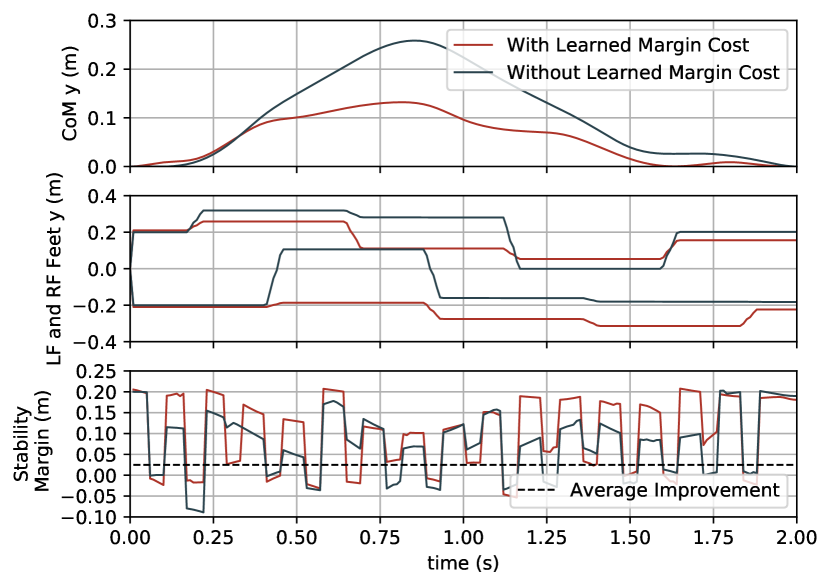
Figure 17: Trajectories referring to two motion plans of Anymal B on flat terrain optimized using TOWR with (blue) and without (red) the cost on the learned stability margin. We can see that maximizing the learned stability margin leads to a decrease in unnecessary base motions (upper plot) and in a larger stance (mid plot). These two elements together lead to an average improvement of the stability margin of about 2.5 cm (lower plot).

In our preliminary experiments, we observed that introducing the stability margin reward term in an environment setup with a simple reward function results in reduced base accelerations. As shown in Movie S5, a locomotion policy obtained using the reward function $-(0.7-{}_{B}v_{{WB}_{x}})^{2}$, is significantly more aggressive compared to the reward function augmented using the stability margin. This reward function can further be tuned to obtain the desired locomotion behavior. In our RL environment setups, we use the stability margin in our reward function to encourage the RL agents to perform less aggressive maneuvers in order to maximize the stability metric.

We extended this work on rapid dynamic stability estimation for use with OC and RL based approaches. The detailed network training and deployment description can be found in [39].

VI-C Cost Map

In order to drive the RL footstep planner to generate desired feet positions which avoid terrain edges, we compute a penalty based on the cost map obtained using the 1^st and 2^nd order derivatives of the elevation map local to the feet positions within a deviation of $\pm$0.065\text{\,}\mathrm{m}$$ along $\mathbf{e}_{x}^{F}$ and $\mathbf{e}_{y}^{F}$ represented by $\mathbf{M}_{F_{i}}:\mathbb{R}^{2}\times\mathbb{R}\rightarrow\mathbb{R}^{27\times 27}$ for foot $i$ sampled at a resolution of $0.005\text{\,}\mathrm{m}$. We compute the cost map by performing operations in the following order:

1. Smoothing: $\mathbf{C}_{\mathbf{M}}(r_{F_{xy},i})\leftarrow\mathcal{C}(\mathbf{M}_{F_{i}},k_{s})$ where

   $$k_{s}=\begin{bmatrix}0.1&0.1&0.1\\ 0.1&0.2&0.1\\ 0.1&0.1&0.1\\ \end{bmatrix}$$

2. Approximation of second order derivative using Laplacian kernel: $\mathbf{C}_{\mathbf{M}}(r_{F_{xy},i})\leftarrow\mathcal{C}(\mathbf{C}_{\mathbf{M}}(r_{F_{xy},i}),k_{l})$ where

   $$k_{l}=\begin{bmatrix}-1&-1&-1\\ -1&8&-1\\ -1&-1&-1\\ \end{bmatrix}$$

3. Modulus of the cost map to represent terrain edges without direction information: $\mathbf{C}_{\mathbf{M}}(r_{F_{xy},i})\leftarrow abs(\mathbf{C}_{\mathbf{M}}(r_{F_{xy},i}))$

4. Estimation of deviation in heights along the edges using blurring kernel: $\mathbf{C}_{\mathbf{M}}(r_{F_{xy},i})\leftarrow\mathcal{C}(\mathbf{C}_{\mathbf{M}}(r_{F_{xy},i}),k_{b})$

   $$k_{b}=\frac{1}{9}\times\begin{bmatrix}1&1&1\\ 1&1&1\\ 1&1&1\\ \end{bmatrix}$$

5. Circular distance filtering such that terrain edge at $\mathbf{M}_{F_{i}}(r_{F_{xy},i})$ has the maximum weighting for computing the cost penalty. This weight decreases with increase in the radial deviation from the center of the feet $r_{F_{xy},i}$. The circular distance filter can be represented as a matrix $\mathbf{M}_{c}\in\mathbb{R}^{21\times 21}$ where the center $\mathbf{M}_{c}(r_{F_{xy},i})=1$ and $\mathbf{M}_{c}(\hat{r}_{F_{xy},i})=max(0.05-||\hat{r}_{F_{xy},i}-r_{F_{xy},i}||,0)/0.05$. The cost map is then modified by performing an element-wise product: $\mathbf{C}_{\mathbf{M}}(r_{F_{xy},i})\leftarrow{M}_{c}\odot\mathbf{C}_{\mathbf{M}}(r_{F_{xy},i})$

Note that, we start with $\mathbf{M}_{F_{i}}:\mathbb{R}^{2}\times\mathbb{R}\rightarrow\mathbb{R}^{27\times 27}$ which corresponds to an area of $(2\times 0.065)\times(2\times 0.065)\,$${\mathrm{m}}^{2}$, and following the above procedure, we obtain the desired $21\times 21$-dimensional cost map which corresponds to an area of $(2\times 0.05)\times(2\times 0.05)\,$${\mathrm{m}}^{2}$. This reduction is due to the convolutions performed without utilizing additional padding.

Figure 18 shows an example of the cost map on a terrains with bricks and holes. In practice, the whole cost map does not need to be explicitly computed since only the cost at each foot position is needed so the transformation are only applied on small patches around the selected footholds.

(a) Terrain elevation

(b) Elevation smoothing

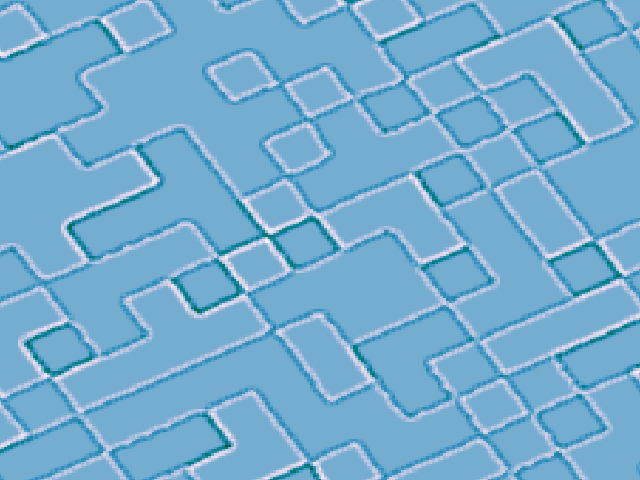
(c) Elevation Laplacian

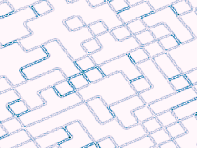
(d) Elevation modulus

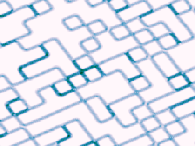
(e) Elevation blurring

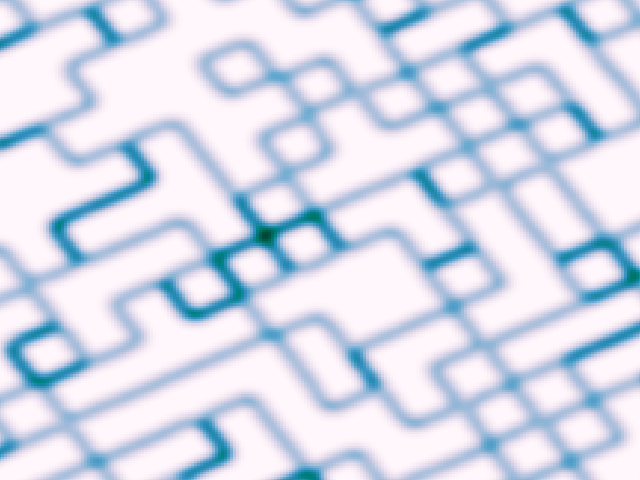
(f) Terrain cost map

Figure 18: Example of computation of the cost map for a bricks terrain. Green color represents upward extrusions corresponding to higher elevation while white color represents downward extrusions. For the cost map, dark blue represents positions with higher cost. Note that, the cost map shown here corresponds to the entire terrain which was obtained by performing convolution using the circular distance filter as opposed to element-wise multiplication which is done for extracting the cost at foot position in $\mathbf{M}_{F_{i}}$.

VI-D Elevation Map Encoding

Our encoder network architecture design is based on the following reasons: (1) the encoder should capture as much information as possible, (2) the encoder forward pass time on the real robots should not exceed the control step time of $2.5\text{\,}\mathrm{ms}$ after the raw elevation map is computed in a parallel thread to avoid change in robot state resulting in feet position tracking drifts. For this, we introduced the unstructured terrain in the dataset for training the autoencoder. We observed that reducing the dimensionality of the latent representation below 96 resulted in poor reconstruction of the unstructured terrain, i.e. the encoder failed to detect the unstructured terrain, and the autoencoder output an almost smooth reconstruction. A forward pass through the encoder network requires approximately $1.7\text{\,}\mathrm{ms}$ on the real robots giving us sufficient time to perform state updates and forward passes through the RL planning and control policy networks.

While training the encoder using the autoencoding strategy, we minimize the loss

$$\mathcal{L}_{\mathbf{M}_{H}}=({\mathbf{M}}_{H}^{n}-{\mathbf{\hat{M}}}_{H}^{n})^{2}\,.$$ (26)

It is a common practice to include a regularization term in this reconstruction loss to discourage overfitting, however, reconstruction from noisy encoder input implies that the auto-encoder is restricted from memorizing the training dataset. Instead, the encoder learns to map the input data to a lower-dimensional manifold which represents the most relevant features of the terrain while getting rid of the additional noise. Hence, it is not necessary for us to introduce additional regularization during training.

VI-E Control Switching

RLOC executes the footstep planner, motion controller and domain adaptive tracker upon initialization. When any of the robot state parameters exceeds a certain threshold described by the activation limit in Table XI, the recovery controller is activated while the footstep planner, motion controller and domain adaptive tracker are deactivated. The recovery controller stabilizes the robot and the active control state switches back to motion planning and whole-body control. This switch is performed when each of the robot state parameters lie within the deactivation limits presented in Table XI.

TABLE XI: Robot state criteria for activating and deactivating the recovery controller. Here $|\cdot|$ refers to the $l_{1}$ norm of a vector, $\mathrm{abs}()$ is the element-wise modulus operator, $\mathrm{max}()$ refers to the maximum element in a vector, $\mathrm{q}_{j}^{n}$ is the vector of nominal joint positions and $(\mathrm{q}_{j}-\mathrm{q}^{n}_{j})_{HAA}$ refers to the vector of elements relating to the four HAA (hip abduction-adduction) joints. HFE refers to hip flexion-extension and KFE refers to knee flexion-extension.

State	Activation Limit	Deactivation Limit
$|\mathrm{v}_{B}|$	20.0	0.5
$|\mathrm{\omega}_{B}|$	5.0	0.5
$\mathrm{max}(\mathrm{abs}((\mathrm{q}_{j}-\mathrm{q}^{n}_{j})_{HAA}))$	$\pi/4$	$\pi/12$
$\mathrm{max}(\mathrm{abs}((\mathrm{q}_{j}-\mathrm{q}^{n}_{j})_{HFE}))$	$\pi/4$	$\pi/12$
$\mathrm{max}(\mathrm{abs}((\mathrm{q}_{j}-\mathrm{q}^{n}_{j})_{KFE}))$	$\pi/3$	$\pi/12$
$|\mathrm{cos}^{-1}(\mathbf{e}_{z}^{B}\cdot\mathbf{e}_{z}^{W})|$	$\pi/3$	$\pi/4$
$|\mathrm{cos}^{-1}(\mathbf{e}_{z}^{B}\cdot\mathbf{e}_{z}^{C})|$	$\pi/4$	$\pi/6$

VI-F Terrain Generation

For terrain generation, we consider several objects such as a staircase, planks, bricks, unstructured sub-terrain and wave sub-terrain. Each terrain contains at least 1 and at most 5 objects. We position and rotate these objects within the terrain area to limit height deviations around close regions and increase the occupancy over the entire terrain, and represent their corresponding heights as elevation in the range of $[0,65535]$ where 0 corresponds to no elevation and 65535 corresponds to an elevation of $2\text{\,}\mathrm{m}$. We automate this generation process using a Python tool which stores a wide range of terrains, 10k in our case, in the form of single channel 16-bit PNG files. These PNGs are then imported in RaiSim as heightmaps. Figure 19 represents the generated terrains for the unstructured ground, stairs, wave and brick objects along with their corresponding visualization in RaiSim.

Figure 19: (top-bottom) represent the terrains comprising of unstructured ground, stairs, wave and brick objects respectively. The left images represent the height maps imported in the RaiSim simulator as shown on the right.

VI-G Actuation Dynamics

The actuator network utilized for training footstep planner and domain adaptive tracker models an adaptive impedance controller which can be represented as

$$\tau_{j}=\mathbf{j}_{R}(\mathrm{q}_{j}^{\ast},\mathrm{q}_{j},\mathrm{\dot{q}}_{j}^{\ast},\mathrm{\dot{q}}_{j},\tau_{j_{FF}},K_{p},K_{d})\ .$$ (27)

The input to the actuator network is thus represented as $j_{s}\in\mathbb{R}^{21}$ such that

$$j_{s}=\langle s_{j_{pe}},s_{j_{ve}},s_{j_{te}},s_{j_{vd}},s_{j_{td}},s_{j_{kp}},s_{j_{kd}}\rangle\ .$$ (28)

The definitions of the input terms are provided in Table XII. This actuator network contains 2 hidden layers with 48 nodes in each of the layers and a 1-dimensional output layer representing the estimate of the joint torque. We perform a forward pass through the network at each time step for each of the 12 joints of the quadruped.

TABLE XII: Actuator input term definitions. Here, $i$ refers to the $i$-th joint. Subscript $t$ refers to the measurement at the current control step and the duration between $t-1$ and $t$ corresponds to $2.5\text{\,}\mathrm{ms}$.

Actuator Network Input Terms

$s_{j_{pe}}=[({\mathrm{q}^{\ast}_{j,i}}_{t}-{\mathrm{q}_{j,i}}_{t})^{T}\ \ ({\mathrm{q}^{\ast}_{j,i}}_{t-4}-{\mathrm{q}_{j,i}}_{t-4})^{T}\ \ ({\mathrm{q}^{\ast}_{j,i}}_{t-8}-{\mathrm{q}_{j,i}}_{t-8})^{T}]^{T}$

$s_{j_{ve}}=[({\mathrm{\dot{q}}^{\ast}_{j,i}}{}_{t}-{\mathrm{\dot{q}}_{j,i}}{}_{t})^{T}\ \ (\mathrm{\dot{q}}^{\ast}_{{j,i}_{t-4}}-\mathrm{\dot{q}}_{{j,i}_{t-4}})^{T}\ \ (\mathrm{\dot{q}}^{\ast}_{{j,i}_{t-8}}-\mathrm{\dot{q}}_{{j,i}_{t-8}})^{T}]^{T}$

$s_{j_{te}}=[({\mathrm{\tau}_{j,i}}_{t}-{\mathrm{\tau}_{{j,i}_{FF}}}_{t})^{T}\ \ ({\mathrm{\tau}_{j,i}}_{t-4}-{\mathrm{\tau}_{{j,i}_{FF}}}_{t-4})^{T}\ \ ({\mathrm{\tau}_{j,i}}_{t-8}-{\mathrm{\tau}_{{j,i}_{FF}}}_{t-8})^{T}]^{T}$

$s_{j_{vd}}=[(\mathrm{\dot{q}}^{\ast}_{{j,i}_{t}})^{T}\ \ (\mathrm{\dot{q}}^{\ast}_{{j,i}_{t-4}})^{T}\ \ (\mathrm{\dot{q}}^{\ast}_{{j,i}_{t-8}})^{T}]^{T}$

$s_{j_{td}}=[{\mathrm{\tau}^{T}_{{j,i}_{FF}}}_{t}\ \ {\mathrm{\tau}^{T}_{{j,i}_{FF}}}_{t-4}\ \ {\mathrm{\tau}^{T}_{{j,i}_{FF}}}_{t-8}]^{T}$

$s_{j_{kp}}=[{K_{p}}^{T}_{t}\ \ {K_{p}}^{T}_{t-4}\ \ {K_{p}}^{T}_{t-8}]^{T}$

$s_{j_{kd}}=[{K_{d}}^{T}_{t}\ \ {K_{d}}^{T}_{t-4}\ \ {K_{d}}^{T}_{t-8}]^{T}$

For training the adaptive impedance actuator network, we collected data from the real system using the dynamic gaits motion controller to track randomly sampled base reference velocities. We recorded the desired relevant input quantities at $400\text{\,}\mathrm{Hz}$ for 12 actuators thus generating a large dataset of 8.64M samples in approximately 30 minutes. However, since the impedance gains depend on the contact state of the robot, during data collection, we obtained sufficient samples for the swing and stance phases. However, during operation, we obtained significantly less samples for the contact-uncertainty state. As a result, using the actuator network trained with the naive supervised learning approach failed to properly track actuation commands for contact-uncertainty states in the simulator causing the motion controller to generate unstable motion tracking commands eventually resulting in failure. To address this, we utilized SMOGN [54, 55] to perform regression over imbalanced data by resampling the dataset generated from the real robot. SMOGN utilizes a random undersampling approach for the majority samples and a synthetic sample generation method for the minority samples. Table XIII presents the mean absolute prediction error comparing the performance of networks trained using a naive supervised learning approach with resampled learning, tested on 50k samples for each of the different sets of PD gains.

TABLE XIII: Effective joint torque prediction error comparing the actuator network performance for training with and without re-sampling of the training dataset using SMOGN. Here $\mu_{e}$ is the mean prediction error and $\sigma_{e}$ is the standard deviation of the prediction error observed over 50k test samples.

	$K_{p}$=8, $K_{d}$=0.1	$K_{p}$=35, $K_{d}$=0.4	$K_{p}$=160, $K_{d}$=0.3
Baseline	$\mu_{e}=0.82$, $\sigma_{e}=0.34$	$\mu_{e}=0.77$, $\sigma_{e}=0.31$	$\mu_{e}=1.73$, $\sigma_{e}=0.85$
SMOGN	$\mu_{e}=0.83$, $\sigma_{e}=0.21$	$\mu_{e}=0.71$, $\sigma_{e}=0.19$	$\mu_{e}=0.96$, $\sigma_{e}=0.39$

VI-H Training

Our motivation for selecting an RL training strategy is based on three main factors: (1) convergence to a desired behavior, (2) sample efficiency, and (3) training time.

We use SAC for training our footstep planning policy mainly for its improved sample efficiency over the widely used TRPO and PPO approaches. In our preliminary experiments for training the footstep planner, we observed that SAC required approximately a fourth of policy iterations for convergence compared to PPO for similar training parameters. For this reason, we decided to use SAC for training our footstep planner.

In the case of domain adaptive tracker, we observed that the stochasticity associated with SAC and PPO necessitated precise hyperparamter tuning, without which the policy failed to exhibit a stable locomotion behavior. Even then, we observed little improvement in domain adaptive tracking. This was largely due to the domain adaptive tracker generating large torques which caused the whole-body controller to aggressively correct for inaccurate tracking resulting in episode termination. Instead, we used TD3 which allowed us to perform exploration using an uncorrelated Gaussian noise. We thus employed a curriculum based exploration strategy where we initialized the policy to output values close to 0s, while also setting a small value for the Gaussian noise standard deviation. As training progressed, we increased the standard deviation. This allowed for stable learning and thus better convergence.

For the recovery controller, we use PPO for 2 main reasons: (1) Prior work on end-to-end state-to-joint RL control has utilized PPO and provided reproducible steps [19], and (2) we observed that, compared to off-policy approaches such as SAC and TD3, PPO required significantly less time to perform policy updates after each episode rollout. Since the footstep planner and domain adaptive tracker employed the motion controller during training, much of the training overhead occurred during simulation rollouts as opposed to policy updates. The recovery controller rollouts were significantly fast since no additional computation, such as motion optimization, was required. PPO thus enabled us to perform faster training even with reduced sample efficiency. In our preliminary experiments, we observed that for each policy iteration, PPO required approximately $3.2\text{\,}\mathrm{s}$ whereas SAC required approximately $13\text{\,}\mathrm{s}$ for similar training parameters. Although it is possible to reduce the policy update duration for SAC with additional parameter tuning, for our test case, PPO still offered policy convergence in less training time than SAC. We therefore decided to use PPO for training the recovery controller.

We trained each of our RL policies on a desktop computer with an Intel i7-8700 processor clocked at $4.0\text{\,}\mathrm{GHz}$ and an NVidia RTX 2080Ti graphics card. The footstep planner Session 1 training time and hyperparameters are shown in Table XIV. For training Session 2, we use the SAC hyperparameters shown in Table XIV for additional 100 policy update iterations requiring roughly 4 hours of training. For training the domain adaptive tracking policy, we use the parameters provided in Table XV, and we use the parameters provided in Table XVI for training the recovery controller.

TABLE XIV: Footstep planner Session 1 training time and hyperparameters.

Parameter	Value
Discount factor, $\gamma$	0.994
Learning rate	1e-4
Buffer size	1e5
Batch size	8192
Prioritized replay buffer	False
Learning starts	24576
Parallel environments, $n_{env}$	24
Soft update coefficient, $\tau$	1e-3
Training frequency	1
Twin Q functions	True
Target entropy	Auto
IGPO $\lambda_{d}$	0.996
IGPO $n_{eps}$	100
Steps per iteration, $l_{eps}$	$1024\times n_{env}$
SAC time per iteration	$\sim$$120\text{\,}\mathrm{s}$
Guided learning time per iteration	$\sim$$105\text{\,}\mathrm{s}$
Total training time	$\sim$$28\text{\,}\mathrm{h}$

TABLE XV: Domain adaptive tracker training time and hyperparameters.

Parameter	Value
Discount factor, $\gamma$	0.998
Learning rate	5e-4
Buffer size	1e6
Batch size	19200
Learning starts	76800
Parallel environments, $n_{env}$	24
Soft update coefficient, $\tau$	5e-3
Prioritized replay	True
Prioritized replay $\alpha$	0.6
Prioritized replay $\beta$	0.6
Twin Q functions	True
Steps per iteration, $l_{eps}$	$3200\times n_{env}$
TD3 time per iteration	$\sim$$4\text{\,}\mathrm{s}$
Total training time	$\sim$$22\text{\,}\mathrm{h}$

TABLE XVI: Recovery controller training time and hyperparameters.

Parameter	Value
Discount factor, $\gamma$	0.996
Learning rate	5e-4
Batch size	115200
Mini-batch size	14400
Parallel environments, $n_{env}$	48
Entropy coefficient	5e-3
Value coefficient	0.25
GAE	True
GAE $\lambda$	0.98
Steps per iteration, $l_{eps}$	$2400\times n_{env}$
PPO time per iteration	$\sim$$3\text{\,}\mathrm{s}$
Total training time	$\sim$$6\text{\,}\mathrm{h}$

Siddhant Gangapurwala completed his Bachelor of Engineering (B.E.) in Electronics from the University of Mumbai in 2016. In 2017, he joined the AIMS program as a doctoral candidate at the University of Oxford. The following year, Siddhant joined the Dynamic Robot Systems (DRS) group of the Oxford Robotics Insitute (ORI) to pursue his DPhil degree with focus on machine learning and optimal control based approaches for robotic locomotion over uneven terrain where he continues to work as a post-doctoral researcher on locomotion, manipulation and loco-manipulation.

Mathieu Geisert received his M. Eng. in Aerospace from Institut Supérieur de l’Aéronautique et de l’Espace SUPAERO (Toulouse, France) in 2013. He then joined the humanoid robotics team, GEPETTO, at LAAS-CNRS (Toulouse, France) where he worked for 5 years in different positions: as an intern, engineer, Ph.D. student and finally as a post doctoral researcher. In 2018, he joined the DRS group as a post-doctoral researcher where his work focused on Planning, Optimal Control and Machine Learning for legged robots. In 2021, Mathieu joined Arrival, London, UK as a robotics research engineer.

Romeo Orsolino completed his B.Sc. in mechanical engineering from the University of Genova in 2013 and his M.Sc. in robotics engineering at the École Centrale de Nantes in 2015. In the same year, he joined DLS at IIT for a Ph.D. focusing on motion planning for legged locomotion in rough terrains. In October 2019, he joined the DRS group as a post-doctoral researcher where he pursued his research on multi-contact motion planning, optimal control, dynamics and perception. In December 2020, Romeo joined Arrival Ltd. where continues to work on perceptive motion planning and control of dynamical systems.

Maurice Fallon studied Electronic Engineering at University College Dublin. His Ph.D. research in the field of acoustic source tracking was carried out in the Engineering Department of the University of Cambridge. After his Ph.D. he moved to MIT as a post doctoral researcher and later research scientist in the Marine Robotics Group (2008-2012). From 2012-2015 he was the perception lead of MIT’s team in the DARPA Robotics Challenge. From 2015, he was a Lecturer at University of Edinburgh where he led research in collaboration with NASA’s humanoid robotics program. He moved to Oxford in April 2017 and took up the Royal Society University Research Fellowship in October 2017.

Ioannis Havoutis is a Departmental Lecturer at the Oxford Robotics Institute. His research combines dynamic whole-body motion planning and control with machine learning, focusing on robots with arms and legs. He received his Ph.D. (2011) and M.Sc. with distinction (2007) from the University of Edinburgh, where he worked on machine learning for motion planning and control of articulated robots. He then joined the Dynamic Legged Systems Lab at the Advanced Robotics Department of IIT, where he led the Locomotion Group within the HyQ team. He was a postdoctoral researcher at the Robot Learning & Interaction Group of the Idiap Research Institute, where he worked on learning complex skills from demonstration.

References

- [1] M. Hutter, C. Gehring, D. Jud, A. Lauber, C. D. Bellicoso, V. Tsounis, J. Hwangbo, K. Bodie, P. Fankhauser, M. Bloesch et al., “Anymal-a highly mobile and dynamic quadrupedal robot,” in 2016 IEEE/RSJ International Conference on Intelligent Robots and Systems (IROS). IEEE, 2016, pp. 38–44.
- [2] E. Ackerman, “Anybotics introduces sleek new anymal c quadruped,” IEEE Spectrum. https://spectrum.ieee.org/automaton/robotics/industrial-robots/anybotics-introduces-sleek-new-anymal-c-quadruped, 2019.
- [3] ——, “North sea deployment shows how quadruped robots can be commercially useful,” IEEE Spectrum. https://spectrum.ieee.org/automaton/robotics/industrial-robots/north-sea-deployment-shows-how-quadruped-robots-can-be-commercially-useful, November 2018.
- [4] H. Kolvenbach, D. Wisth, R. Buchanan, G. Valsecchi, R. Grandia, M. Fallon, and M. Hutter, “Towards autonomous inspection of concrete deterioration in sewers with legged robots,” Journal of Field Robotics, 2020. [Online]. Available: https://onlinelibrary.wiley.com/doi/abs/10.1002/rob.21964
- [5] I. Mordatch, E. Todorov, and Z. Popović, “Discovery of complex behaviors through contact-invariant optimization,” ACM Trans. Graph., vol. 31, no. 4, Jul. 2012. [Online]. Available: https://doi.org/10.1145/2185520.2185539
- [6] C. Mastalli, R. Budhiraja, W. Merkt, G. Saurel, B. Hammoud, M. Naveau, J. Carpentier, L. Righetti, S. Vijayakumar, and N. Mansard, “Crocoddyl: An efficient and versatile framework for multi-contact optimal control,” in 2020 IEEE International Conference on Robotics and Automation (ICRA), 2020, pp. 2536–2542.
- [7] R. Grandia, F. Farshidian, R. Ranftl, and M. Hutter, “Feedback mpc for torque-controlled legged robots,” in 2019 IEEE/RSJ International Conference on Intelligent Robots and Systems (IROS), 2019, pp. 4730–4737.
- [8] R. Full and D. Koditschek, “Templates and anchors: neuromechanical hypotheses of legged locomotion on land,” Journal of Experimental Biology, vol. 202, no. 23, pp. 3325–3332, 1999. [Online]. Available: http://jeb.biologists.org/content/202/23/3325
- [9] S. Kajita, F. Kanehiro, K. Kaneko, K. Yokoi, and H. Hirukawa, “The 3d linear inverted pendulum mode: a simple modeling for a biped walking pattern generation,” in IEEE/RSJ International Conference on Intelligent Robots and Systems (IROS), vol. 1, Oct 2001, pp. 239–246 vol.1.
- [10] I. Poulakakis, E. Papadopoulos, and M. Buehler, “On the stability of the passive dynamics of quadrupedal running with a bounding gait,” The International Journal of Robotics Research, vol. 25, no. 7, pp. 669–687, 2006. [Online]. Available: https://doi.org/10.1177/0278364906066768
- [11] I. Poulakakis and J. W. Grizzle, “The spring loaded inverted pendulum as the hybrid zero dynamics of an asymmetric hopper,” IEEE Transactions on Automatic Control, vol. 54, no. 8, pp. 1779–1793, 2009.
- [12] M. Vukobratović and D. Juric̃ić, “Contribution to the synthesis of biped gait,” Proc. IFAC Symp. Technical and Biological Problem on Control, Erevan, USSR, 1968.
- [13] J. Pratt, J. Carff, S. Drakunov, and A. Goswami, “Capture point: A step toward humanoid push recovery,” pp. 200 – 207, 01 2007.
- [14] D. E. Orin, A. Goswami, and S.-H. Lee, “Centroidal dynamics of a humanoid robot,” Auton. Robots, vol. 35, no. 2-3, pp. 161–176, Oct. 2013. [Online]. Available: http://dx.doi.org/10.1007/s10514-013-9341-4
- [15] H. Dai and R. Tedrake, “Planning robust walking motion on uneven terrain via convex optimization,” in Humanoids, 2016.
- [16] J. Carpentier and N. Mansard, “Multicontact locomotion of legged robots,” IEEE Transactions on Robotics, vol. 34, no. 6, pp. 1441–1460, 2018.
- [17] F. Jenelten, T. Miki, A. E. Vijayan, M. Bjelonic, and M. Hutter, “Perceptive locomotion in rough terrain–online foothold optimization,” IEEE Robotics and Automation Letters, vol. 5, no. 4, pp. 5370–5376, 2020.
- [18] D. Kim, D. Carballo, J. Di Carlo, B. Katz, G. Bledt, B. Lim, and S. Kim, “Vision aided dynamic exploration of unstructured terrain with a small-scale quadruped robot,” in 2020 IEEE International Conference on Robotics and Automation (ICRA). IEEE, 2020, pp. 2464–2470.
- [19] J. Hwangbo, J. Lee, A. Dosovitskiy, D. Bellicoso, V. Tsounis, V. Koltun, and M. Hutter, “Learning agile and dynamic motor skills for legged robots,” Science Robotics, vol. 4, no. 26, 2019. [Online]. Available: https://robotics.sciencemag.org/content/4/26/eaau5872
- [20] J. Lee, J. Hwangbo, and M. Hutter, “Robust recovery controller for a quadrupedal robot using deep reinforcement learning,” arXiv preprint arXiv:1901.07517, 2019.
- [21] S. Gangapurwala, A. Mitchell, and I. Havoutis, “Guided constrained policy optimization for dynamic quadrupedal robot locomotion,” IEEE Robotics and Automation Letters, vol. 5, no. 2, pp. 3642–3649, 2020.
- [22] X. B. Peng, E. Coumans, T. Zhang, T.-W. Lee, J. Tan, and S. Levine, “Learning agile robotic locomotion skills by imitating animals,” arXiv preprint arXiv:2004.00784, 2020.
- [23] Z. Xie, G. Berseth, P. Clary, J. Hurst, and M. van de Panne, “Feedback control for cassie with deep reinforcement learning,” in 2018 IEEE/RSJ International Conference on Intelligent Robots and Systems (IROS). IEEE, 2018, pp. 1241–1246.
- [24] S. Levine and V. Koltun, “Guided policy search,” in International Conference on Machine Learning, 2013, pp. 1–9.
- [25] T. Haarnoja, S. Ha, A. Zhou, J. Tan, G. Tucker, and S. Levine, “Learning to walk via deep reinforcement learning,” arXiv preprint arXiv:1812.11103, 2018.
- [26] Y. Yang, K. Caluwaerts, A. Iscen, T. Zhang, J. Tan, and V. Sindhwani, “Data efficient reinforcement learning for legged robots,” in Conference on Robot Learning, 2020, pp. 1–10.
- [27] J. Tobin, R. Fong, A. Ray, J. Schneider, W. Zaremba, and P. Abbeel, “Domain randomization for transferring deep neural networks from simulation to the real world,” in 2017 IEEE/RSJ International Conference on Intelligent Robots and Systems (IROS). IEEE, 2017, pp. 23–30.
- [28] V. Tsounis, M. Alge, J. Lee, F. Farshidian, and M. Hutter, “Deepgait: Planning and control of quadrupedal gaits using deep reinforcement learning,” IEEE Robotics and Automation Letters, vol. 5, no. 2, pp. 3699–3706, 2020.
- [29] J. Lee, J. Hwangbo, L. Wellhausen, V. Koltun, and M. Hutter, “Learning quadrupedal locomotion over challenging terrain,” Science robotics, vol. 5, no. 47, 2020.
- [30] T. Miki, J. Lee, J. Hwangbo, L. Wellhausen, V. Koltun, and M. Hutter, “Learning robust perceptive locomotion for quadrupedal robots in the wild,” Science Robotics, vol. 7, no. 62, p. eabk2822, 2022.
- [31] C. D. Bellicoso, F. Jenelten, C. Gehring, and M. Hutter, “Dynamic locomotion through online nonlinear motion optimization for quadrupedal robots,” IEEE Robotics and Automation Letters, vol. 3, no. 3, pp. 2261–2268, 2018.
- [32] R. S. Sutton, A. G. Barto et al., Introduction to reinforcement learning. MIT press Cambridge, 1998, vol. 135.
- [33] P. Fankhauser, M. Bloesch, and M. Hutter, “Probabilistic terrain mapping for mobile robots with uncertain localization,” IEEE Robotics and Automation Letters (RA-L), vol. 3, no. 4, pp. 3019–3026, 2018.
- [34] N. Rudin, D. Hoeller, P. Reist, and M. Hutter, “Learning to walk in minutes using massively parallel deep reinforcement learning,” in Conference on Robot Learning. PMLR, 2022, pp. 91–100.
- [35] A. Iscen, K. Caluwaerts, J. Tan, T. Zhang, E. Coumans, V. Sindhwani, and V. Vanhoucke, “Policies modulating trajectory generators,” in Conference on Robot Learning. PMLR, 2018, pp. 916–926.
- [36] C. D. Bellicoso, F. Jenelten, P. Fankhauser, C. Gehring, J. Hwangbo, and M. Hutter, “Dynamic locomotion and whole-body control for quadrupedal robots,” in 2017 IEEE/RSJ International Conference on Intelligent Robots and Systems (IROS). IEEE, 2017, pp. 3359–3365.
- [37] F. Jenelten, J. Hwangbo, F. Tresoldi, C. D. Bellicoso, and M. Hutter, “Dynamic locomotion on slippery ground,” IEEE Robotics and Automation Letters, vol. 4, no. 4, pp. 4170–4176, 2019.
- [38] R. Orsolino, M. Focchi, S. Caron, G. Raiola, V. Barasuol, and C. Semini, “Feasible region: an actuation-aware extension of the support region,” IEEE Transactions on Robotics (TRO), 2020.
- [39] R. Orsolino, S. Gangapurwala, O. Melon, M. Geisert, I. Havoutis, and M. Fallon, “Rapid stability margin estimation for contact-rich locomotion,” 2021.
- [40] T. Haarnoja, A. Zhou, P. Abbeel, and S. Levine, “Soft actor-critic: Off-policy maximum entropy deep reinforcement learning with a stochastic actor,” arXiv preprint arXiv:1801.01290, 2018.
- [41] E. Liang, R. Liaw, R. Nishihara, P. Moritz, R. Fox, K. Goldberg, J. E. Gonzalez, M. I. Jordan, and I. Stoica, “RLlib: Abstractions for distributed reinforcement learning,” in International Conference on Machine Learning (ICML), 2018.
- [42] J. Schulman, S. Levine, P. Abbeel, M. Jordan, and P. Moritz, “Trust region policy optimization,” in International conference on machine learning, 2015, pp. 1889–1897.
- [43] J. Schulman, F. Wolski, P. Dhariwal, A. Radford, and O. Klimov, “Proximal policy optimization algorithms,” arXiv preprint arXiv:1707.06347, 2017.
- [44] T. Haarnoja, A. Zhou, K. Hartikainen, G. Tucker, S. Ha, J. Tan, V. Kumar, H. Zhu, A. Gupta, P. Abbeel et al., “Soft actor-critic algorithms and applications,” arXiv preprint arXiv:1812.05905, 2018.
- [45] S. Fujimoto, H. Hoof, and D. Meger, “Addressing function approximation error in actor-critic methods,” in International Conference on Machine Learning, 2018, pp. 1582–1591.
- [46] J. Hwangbo, J. Lee, and M. Hutter, “Per-contact iteration method for solving contact dynamics,” IEEE Robotics and Automation Letters, vol. 3, no. 2, pp. 895–902, 2018.
- [47] S. Gangapurwala, M. Geisert, R. Orsolino, M. Fallon, and I. Havoutis, “Real-time trajectory adaptation for quadrupedal locomotion using deep reinforcement learning,” in Proceedings of the International Conference on Robotics and Automation (ICRA). Institute of Electrical and Electronics Engineers, 2021.
- [48] X. Glorot and Y. Bengio, “Understanding the difficulty of training deep feedforward neural networks,” in Proceedings of the thirteenth international conference on artificial intelligence and statistics, 2010, pp. 249–256.
- [49] N. Koenig and A. Howard, “Design and use paradigms for gazebo, an open-source multi-robot simulator,” in 2004 IEEE/RSJ International Conference on Intelligent Robots and Systems (IROS)(IEEE Cat. No. 04CH37566), vol. 3. IEEE, 2004, pp. 2149–2154.
- [50] R. Smith et al., “Open dynamics engine,” 2005.
- [51] J. Nocedal and S. Wright, Numerical optimization. Springer Science & Business Media, 2006.
- [52] T. Bretl and S. Lall, “Testing static equilibrium for legged robots,” IEEE Transactions on Robotics, 2008.
- [53] A. W. Winkler, C. D. Bellicoso, M. Hutter, and J. Buchli, “Gait and Trajectory Optimization for Legged Systems through Phase-based End-Effector Parameterization,” IEEE Robotics and Automation Letters (RA-L), pp. 1–1, 2018. [Online]. Available: http://ieeexplore.ieee.org/document/8283570/
- [54] P. Branco, L. Torgo, and R. P. Ribeiro, “Smogn: a pre-processing approach for imbalanced regression,” in First International Workshop on Learning with Imbalanced Domains: Theory and Applications, 2017, pp. 36–50.
- [55] N. Kunz, “SMOGN: Synthetic minority over-sampling technique for regression with gaussian noise,” 2020. [Online]. Available: https://pypi.org/project/smogn/