Several Approximate Algorithms for Sparse Best Rank-$1$ Approximation to Higher-Order Tensors

Abstract

Sparse tensor best rank-1 approximation (BR1Approx), which is a sparsity generalization of the dense tensor BR1Approx, and is a higher-order extension of the sparse matrix BR1Approx, is one of the most important problems in sparse tensor decomposition and related problems arising from statistics and machine learning. By exploiting the multilinearity as well as the sparsity structure of the problem, four polynomial-time approximation algorithms are proposed, which are easily implemented, of low computational complexity, and can serve as initial procedures for iterative algorithms. In addition, theoretically guaranteed approximation lower bounds are derived for all the algorithms. We provide numerical experiments on synthetic and real data to illustrate the efficiency and effectiveness of the proposed algorithms; in particular, serving as initialization procedures, the approximation algorithms can help in improving the solution quality of iterative algorithms while reducing the computational time.

Key words: tensor; sparse; rank-1 approximation; approximation algorithm; approximation bound

1 Introduction

In the big data era, people often face intrinsically multi-dimensional, multi-modal and multi-view data-sets that are too complex to be processed and analyzed by traditional data mining tools based on vectors or matrices. Higher-order tensors (hypermatrices) naturally can represent such complex data sets. Tensor decomposition tools, developed for understanding tensor-based data sets, have shown the power in various fields such as signal processing, image processing, statistics, and machine learning; see the surveys [16, 6, 8, 5, 29, 4].

In high dimensional data-sets, another structure that cannot be ignored is the sparsity. Sparsity tensor examples come from clustering problems, online advertising, web link analysis, ranking of authors based on citations [32, 31, 26, 17, 24], and so on. Therefore, recent advances incorporate sparsity into tensor decomposition models and tensor-based statistics and machine learning problems [3, 26, 32, 1, 21, 30, 38, 35]; just to name a few. As pointed out by Allen [1], introducing sparsity into tensor problems is desirable for feature selection, for compression, for statistical consistency, and for better visualization and interpretation of the data analysis results.

In (dense) tensor decomposition and related tensor models and problems, the best rank-1 approximation (BR1Approx) is one of the most important and fundamental problems [10, 28]. Just as the dense counterpart, the sparse tensor BR1Approx serves as a keystone in the computation of sparse tensor decomposition and related sparse tensor models [32, 30, 1, 35, 26]. Roughly speaking, the sparse tensor BR1Approx is to find a projection of a given data tensor onto the set of sparse rank-1 tensors in the sense of Euclidean distance. This is equivalent to maximizing a multilinear function over both unit sphere and $\ell_{0}$ constraints; mathematical models will be detailed in Section 2. Such a problem also closely connects to the sparse tensor spectral norm defined in [32, 30].

For (dense) tensor BR1Approx, several methods have been proposed; e.g., power methods [18, 10], approximation algorithms [13, 39, 12], and convex relaxations [25, 15, 37]. For sparse matrix BR1Approx, solution methods have been studied extensively in the context of sparse PCA and sparse SVD [40, 36]; see, e.g., iterative methods [20, 36], approximation algorithms [2, 11], and semidefinite relaxation [9]; just to name a few. For sparse tensor BR1Approx, in the context of sparse tensor decomposition, Allen [1] first studied models and iterative algorithms based on $\ell_{1}$ regularization in the literature, whereas Sun et al. [32] developed $\ell_{0}$-based models and algorithms, and analyzed their statistical performance. Wang et al. [35] considered another $\ell_{1}$ regularized model and algorithm, which is different from [1]. In the study of co-clustering, Papalexakis et al. [26] proposed alternating minimization methods for nonnegative sparse tensor BR1Approx.

For nonconvex and NP-hard problems, approximation algorithms are nevertheless encouraged. However, in the context of sparse tensor BR1Approx problems, little attention was paid to this type of algorithms. To fill this gap, by fully exploiting the multilinearity and sparsity of the model, we develop four polynomial-time approximation algorithms, some extending their matrix or dense tensor counterparts; in particular, the last algorithm, which is the most efficient one, is even new when reducing to the matrix or dense tensor cases. The proposed algorithms are easily implemented, and the computational complexity is not high: the most expensive execution is, if necessary, to only compute the largest singular vector pairs of certain matrices. Therefore, the algorithms are able to serve as initialization procedures for iterative algorithms. Moreover, for each algorithm, we derive theoretically guaranteed approximation lower bounds. Experiments on synthetic as well as real data show the usefulness of the introduced algorithms.

The rest of this work is organized as follows. Sect. 2 introduces the sparse tensor BR1Approx model. Approximation algorithms are presented in Sect. 3. Numerical results are illustrated in Sect. 4. Sect. 5 draws some conclusions.

2 Sparse Tensor Best Rank-1 Approximation

Throughout this work, vectors are written as $(\mathbf{x},\mathbf{y},\ldots)$, matrices correspond to $(A,B,\ldots)$, and tensors are written as $(\mathcal{A},\mathcal{B},\cdots)$. $\mathbb{R}^{n_{1}\times\cdots\times n_{d}}$ denotes the space of $n_{1}\times\cdots\times n_{d}$ real tensors. For two tensors $\mathcal{A},\mathcal{B}$ of the same size, their inner product $\langle\mathcal{A},\mathcal{B}\rangle$ is given by the sum of entry-wise product. The Frobenius norm of $\mathcal{A}$ is defined by $\|\mathcal{A}\|_{F}=\langle\mathcal{A},\mathcal{A}\rangle^{1/2}$. $\circ$ denotes the outer product; in particular, for $\mathbf{x}_{j}\in\mathbb{R}^{n_{j}}$, $j=1,\ldots,d$, $\mathbf{x}_{1}\circ\cdots\circ\mathbf{x}_{d}$ denotes a rank-1 tensor in $\mathbb{R}^{n_{1}\times\cdots\times n_{d}}$. $\left\|\mathbf{x}\right\|_{0}$ represents the number of nonzero entries of a vector $\mathbf{x}$.

Given $\mathcal{A}\in\mathbb{R}^{n_{1}\times\cdots\times n_{d}}$ with $d\geq 3$, the tensor BR1Approx consists of finding a set of vectors $\mathbf{x}_{1},\ldots,\mathbf{x}_{d}$, such that

$$\min_{\lambda\in\mathbb{R},\mathbf{x}_{j}\in\mathbb{R}^{n_{j}},1\leq j\leq d}~{}\left\|\lambda\cdot\mathbf{x}_{1}\circ\cdots\circ\mathbf{x}_{d}-\mathcal{A}\right\|_{F}^{2}~{}{\rm s.t.}\left\|\mathbf{x}_{j}\right\|=1,~{}1\leq j\leq d,$$ (2.1)

When $\mathcal{A}$ is sparse, it may be necessary to also investigate the sparsity of the latent factors $\mathbf{x}_{j}$, $1\leq j\leq d$. Assume that the true sparsity level of each latent factors is known a prior, or can be estimated; then the sparse tensor BR1Approx can be modeled as follows [32]:

$$\min_{\lambda\in\mathbb{R},\mathbf{x}_{j}\in\mathbb{R}^{n_{j}},1\leq j\leq d}~{}\left\|\lambda\cdot\mathbf{x}_{1}\circ\cdots\circ\mathbf{x}_{d}-\mathcal{A}\right\|_{F}^{2}~{}{\rm s.t.}\left\|\mathbf{x}_{j}\right\|=1,~{}\left\|\mathbf{x}_{j}\right\|_{0}\leq r_{j},1\leq j\leq d,$$ (2.2)

where $1\leq r_{j}\leq n_{j}$ are positive integers standing for the sparsity level. Allen [1] and Wang et al. [35] proposed $\ell_{1}$ regularized models for sparse tensor BR1Approx problems.

Since $\mathbf{x}_{j}$’s are normalized in (2.2), we have

$$\left\|\lambda\mathbf{x}_{1}\circ\cdots\circ\mathbf{x}_{d}-\mathcal{A}\right\|_{F}^{2} = \left\|\mathcal{A}\right\|_{F}^{2}-2\lambda\left\langle\mathcal{A},\mathbf{x}_{1}\circ\cdots\circ\mathbf{x}_{d}\right\rangle+\lambda^{2}\prod^{d}_{j=1}\nolimits\left\|\mathbf{x}_{j}\right\|^{2}$$

$$= \left\|\mathcal{A}\right\|_{F}^{2}-2\lambda\left\langle\mathcal{A},\mathbf{x}_{1}\circ\cdots\circ\mathbf{x}_{d}\right\rangle+\lambda^{2},$$

minimizing which with respect to $\lambda$ gives $\lambda=\left\langle\mathcal{A},\mathbf{x}_{1}\circ\cdots\circ\mathbf{x}_{d}\right\rangle$, and so

$$\left\|\lambda\mathbf{x}_{1}\circ\cdots\mathbf{x}_{d}-\mathcal{A}\right\|_{F}^{2}=\left\|\mathcal{A}\right\|_{F}^{2}-\left\langle\mathcal{A},\mathbf{x}_{1}\circ\cdots\circ\mathbf{x}_{d}\right\rangle^{2}.$$

Due to the multilinearity of $\left\langle\mathcal{A},\mathbf{x}_{1}\circ\cdots\circ\mathbf{x}_{d}\right\rangle$, $\left\langle\mathcal{A},\mathbf{x}_{1}\circ\cdots\circ\mathbf{x}_{d}\right\rangle^{2}$ is maximized if and only if $\left\langle\mathcal{A},\mathbf{x}_{1}\circ\cdots\circ\mathbf{x}_{d}\right\rangle$ is maximized. Thus (2.2) can be equivalently recast as

$$\boxed{\max_{\mathbf{x}_{j},1\leq j\leq d}\nolimits~{}\left\langle\mathcal{A},\mathbf{x}_{1}\circ\cdots\circ\mathbf{x}_{d}\right\rangle~{}{\rm s.t.}~{}\left\|\mathbf{x}_{j}\right\|=1,\left\|\mathbf{x}_{j}\right\|_{0}\leq r_{j},1\leq j\leq d.}$$ (2.3)

This is the main model to be focused on. When $r_{j}=n_{j}$, (2.3) boils down exactly to the tensor singular value problem [19]. Thus (2.2) can be regarded as a sparse tensor singular value problem.

When $r_{j}=n_{j}$, (2.3) is already NP-hard in general [14]; on the other hand, when $d=2$ and $\mathbf{x}_{1}=\mathbf{x}_{2}$, it is also NP-hard [22]. Therefore, we may deduce that (2.3) is also NP-hard, whose NP-hardness comes from two folds: the multilinearity of the objective function, and the sparsity constraints. In view of this, approximation algorithms for solving (2.3) are necessary.

In the rest of this work, to simplify notations, we denote

$$\mathcal{A}\mathbf{x}_{1}\cdots\mathbf{x}_{d}:=\left\langle\mathcal{A},\mathbf{x}_{1}\circ\cdots\circ\mathbf{x}_{d}\right\rangle.$$

In addition, we also use the following notation to denote the partial gradients of $\mathcal{A}\mathbf{x}_{1}\cdots\mathbf{x}_{d}$ with respect to $\mathbf{x}_{j}$:

$$\mathcal{A}\mathbf{x}_{1}\cdots\mathbf{x}_{j-1}\mathbf{x}_{j+1}\cdots\mathbf{x}_{d}~{}=~{}\nabla_{\mathbf{x}_{j}}\mathcal{A}\mathbf{x}_{1}\cdots\mathbf{x}_{d}\in\mathbb{R}^{n_{j}},~{}1\leq j\leq d.$$

For example, $(\mathcal{A}\mathbf{x}_{2}\cdots\mathbf{x}_{d})_{i_{1}}=\sum^{n_{2},\ldots,n_{d}}_{i_{2}=1,\ldots,i_{d}=1}\mathcal{A}_{i_{1}i_{2}\cdots i_{d}}\mathbf{x}_{2,i_{2}}\cdots\mathbf{x}_{d,i_{d}}$, where we write $\mathbf{x}_{j}:=[x_{j,1},\ldots,x_{j,n_{j}}]^{\top}$. The partial Hessian of $\mathcal{A}\mathbf{x}_{1}\cdots\mathbf{x}_{d}$ with respect to $\mathbf{x}_{d-1}$ and $\mathbf{x}_{d}$ is denoted as:

$$\mathcal{A}\mathbf{x}_{1}\cdots\mathbf{x}_{d-2}=\nabla_{\mathbf{x}_{d-1},\mathbf{x}_{d}}\mathcal{A}\mathbf{x}_{1}\cdots\mathbf{x}_{d}\in\mathbb{R}^{n_{d-1}\times n_{d}},$$

with $(\mathcal{A}\mathbf{x}_{1}\cdots\mathbf{x}_{d-2})_{i_{d-1},i_{d}}=\sum^{n_{1},\ldots,n_{d-2}}_{i_{1}=1,\ldots,i_{d-2}=1}\mathcal{A}_{i_{1}\cdots i_{d-1}i_{d}}\mathbf{x}_{1,i_{1}}\cdots\mathbf{x}_{d-2,i_{d-2}}$.

3 Approximation Algorithms and Approximation Bounds

Four approximation algorithms are proposed in this section, all of which admit theoretical lower bounds. We first present some preparations used in this section. For any nonzero $\mathbf{a}\in\mathbb{R}^{n}$, $1\leq r\leq n$, denote $\left[\mathbf{a}\right]^{\downarrow,r}\in\mathbb{R}^{n}$ as a truncation of $\mathbf{a}$ as

$$\left[\mathbf{a}\right]^{\downarrow,r}_{i}=\left\{\begin{array}[]{lr}a_{i},&{\rm if}~{}|a_{i}|{\rm~{}is~{}one~{}of~{}the~{}}r~{}{\rm largest~{}(in~{}magnitude)~{}entries~{}of~{}}\mathbf{a},\\ 0,&{\rm otherwise}.\end{array}\right.$$

In particular, if $a_{i_{1}}$, $a_{i_{2}}$, $a_{i_{3}},\ldots$ are respectively the $r$-, $(r+1)$-, $(r+2)$-, $\ldots$ largest entries (in magnitude) with $i_{1}<i_{2}<i_{3}<\cdots$, and $|a_{i_{1}}|=|a_{i_{2}}|=|a_{i_{3}}|=\cdots$, then we set $\left[\mathbf{a}\right]^{\downarrow,r}_{i_{1}}=a_{i_{1}}$ and $\left[\mathbf{a}\right]^{\downarrow,r}_{i_{2}}=\left[\mathbf{a}\right]^{\downarrow,r}_{i_{3}}=\cdots=0$. Thus $\left[\mathbf{a}\right]^{\downarrow,r}$ is uniquely defined. We can see that $\left[\mathbf{a}\right]^{\downarrow,r}$ is a best $r$-approximation to $\mathbf{a}$ [20, Proposition 4.3], i.e.,

$$\left[\mathbf{a}\right]^{\downarrow,r}\in\arg\min_{\left\|\mathbf{x}\right\|_{0}\leq r}\left\|\mathbf{x}-\mathbf{a}\right\|~{}~{}\Leftrightarrow~{}~{}\frac{\left[\mathbf{a}\right]^{\downarrow,r}}{\|\left[\mathbf{a}\right]^{\downarrow,r}\|}\in\arg\max_{\left\|\mathbf{x}\right\|=1,\left\|\mathbf{x}\right\|_{0}\leq r}\mathbf{a}^{\top}\mathbf{x}.$$ (3.4)

It is not hard to see that the following proposition holds.

Proposition 3.1.

Let $\mathbf{a}\in\mathbb{R}^{n}$, $\mathbf{a}\neq 0$ and let $\mathbf{a}^{0}=\left[\mathbf{a}\right]^{\downarrow,r}/\|\left[\mathbf{a}\right]^{\downarrow,r}\|$ with $1\leq r\leq n$. Then

$$\left\langle\mathbf{a},\mathbf{a}^{0}\right\rangle\geq\sqrt{\frac{r}{n}}\left\|\mathbf{a}\right\|.$$

Let $\lambda_{\max}(\cdot)$ denote the largest singular value of a given matrix. The following lemma is important.

Lemma 3.1.

Given a nonzero $A\in\mathbb{R}^{m\times n}$, with $(\mathbf{y},\mathbf{z})$ being the normalized singular vector pair corresponding to $\lambda_{\max}(A)$. Let $\mathbf{z}^{0}=\left[\mathbf{z}\right]^{\downarrow,r}/\|\left[\mathbf{z}\right]^{\downarrow,r}\|$ with $1\leq r\leq n$. Then there holds

$$\small\left\|A\mathbf{z}^{0}\right\|\geq\sqrt{\frac{r}{n}}\lambda_{\max}(A).$$

Proof.

From the definition of $\mathbf{z}$, we see that $\left\|A\mathbf{z}\right\|=\lambda_{\max}(A)$ and $A^{\top}A\mathbf{z}=\lambda_{\max}^{2}(A)\mathbf{z}$. Therefore,

$$\lambda_{\max}(A)\left\|A\mathbf{z}^{0}\right\| = \left\|A\mathbf{z}^{0}\right\|\cdot\left\|A{\mathbf{z}}\right\|$$

$$\geq \left\langle A\mathbf{z}^{0},A{\mathbf{z}}\right\rangle$$

$$= \lambda_{\max}(A)\cdot\left\langle A\mathbf{z}^{0},{\mathbf{y}}\right\rangle=\lambda^{2}_{\max}(A)\cdot\left\langle\mathbf{z}^{0},{\mathbf{z}}\right\rangle$$

$$\geq \sqrt{\frac{r}{n}}\lambda^{2}_{\max}(A),$$

where the last inequality follows from Proposition 3.1, the definition of $\mathbf{z}^{0}$, and that $\left\|{\mathbf{z}}\right\|=1$. This completes the proof. ∎

3.1 The first algorithm

To illustrate the first algorithm, we denote $\mathbf{e}_{j}^{i_{j}}\in\mathbb{R}^{n_{j}}$, $1\leq i_{j}\leq n_{j}$, $j=1,\ldots,d$, as standard basis vectors in $\mathbb{R}^{n_{j}}$. For example, $\mathbf{e}_{2}^{1}$ is a vector in $\mathbb{R}^{n_{2}}$ with the first entry being one and the remaining ones being zero. Denote $\boldsymbol{r}:=(r_{1},\ldots,r_{d})$; without loss of generality, we assume that $r_{1}\leq\cdots\leq r_{d}$.

$$\noindent{\rm Algorithm}~{}(\mathbf{x}^{0}_{1},\ldots,\mathbf{x}^{0}_{d})={\rm approx\_alg}(\mathcal{A},\boldsymbol{r})$$ (A) 1. For each $i_{j}=1,\ldots,n_{j}$, $j=1,\ldots,d-1$, compute $\left[\mathcal{A}\mathbf{e}_{1}^{i_{1}}\cdots\mathbf{e}_{d-1}^{i_{d-1}}\right]^{\downarrow,r_{d}}\in\mathbb{R}^{n_{d}}$. 2. Let $(\bar{i}_{1},\ldots,\bar{i}_{d-1})$ be a tuple of indices such that $$\left\|\left[\mathcal{A}\mathbf{e}_{1}^{\bar{i}_{1}}\cdots\mathbf{e}_{d-1}^{\bar{i}_{d-1}}\right]^{\downarrow,r_{d}}\right\|=\max_{1\leq i_{j}\leq n_{j},1\leq j\leq d-1}\left\|\left[\mathcal{A}\mathbf{e}_{1}^{i_{1}}\cdots\mathbf{e}_{d-1}^{i_{d-1}}\right]^{\downarrow,r_{d}}\right\|;$$ denote $\bar{\mathbf{x}}^{0}_{d}:=\left[\mathcal{A}\mathbf{e}_{1}^{\bar{i}_{1}}\cdots\mathbf{e}_{d-1}^{\bar{i}_{d-1}}\right]^{\downarrow,r_{d}}$ and $\mathbf{x}_{d}^{0}:=\bar{\mathbf{x}}^{0}_{d}/\|\bar{\mathbf{x}}^{0}_{d}\|$. 3. Sequentially update $\displaystyle\bar{\mathbf{x}}^{0}_{d-1}$ $\displaystyle=$ $\displaystyle\left[\mathcal{A}\mathbf{e}_{1}^{\bar{i}_{1}}\cdots\mathbf{e}_{d-2}^{\bar{i}_{d-2}}\mathbf{x}^{0}_{d}\right]^{\downarrow,r_{d-1}},\mathbf{x}^{0}_{d-1}=\bar{\mathbf{x}}^{0}_{d-1}/\left\|\bar{\mathbf{x}}^{0}_{d-1}\right\|,$ $\displaystyle\bar{\mathbf{x}}^{0}_{d-2}$ $\displaystyle=$ $\displaystyle\left[\mathcal{A}\mathbf{e}_{1}^{\bar{i}_{1}}\cdots\mathbf{e}_{d-3}^{\bar{i}_{d-3}}\mathbf{x}^{0}_{d-1}\mathbf{x}^{0}_{d}\right]^{\downarrow,r_{d-2}},\mathbf{x}^{0}_{d-2}=\bar{\mathbf{x}}^{0}_{d-2}/\left\|\bar{\mathbf{x}}^{0}_{d-2}\right\|,$ $\displaystyle\vdots$ $\displaystyle\bar{\mathbf{x}}^{0}_{1}$ $\displaystyle=$ $\displaystyle\left[\mathcal{A}\mathbf{x}^{0}_{2}\cdots\mathbf{x}^{0}_{d}\right]^{\downarrow,r_{1}},\mathbf{x}^{0}_{1}=\bar{\mathbf{x}}^{0}_{1}/\left\|\bar{\mathbf{x}}^{0}_{1}\right\|.$ 4. Return $(\mathbf{x}^{0}_{1},\ldots,\mathbf{x}^{0}_{d})$.

It is clear that $\mathcal{A}\mathbf{e}_{1}^{i_{1}}\cdots\mathbf{e}_{d-1}^{i_{d-1}}$’s are mode-$d$ fibers of $\mathcal{A}$. For the definition of fibers, one can refer to [16]; following the Matlab notation we have $\mathcal{A}(i_{1},\ldots,i_{d-1},:)=\mathcal{A}\mathbf{e}_{1}^{i_{1}}\cdots\mathbf{e}_{d-1}^{i_{d-1}}$. Algorithm A is a straightforward extension of [2, Algorithm 1] for sparse symmetric matrix PCA to higher-order tensor cases. Intuitively, the first two steps of Algorithm A enumerate all the mode-$d$ fibers of $\mathcal{A}$, such that the select one admits the largest length with respect to its largest $r_{d}$ entries (in magnitude). $\mathbf{x}^{0}_{d}$ is then given by the normalization of this fiber. Then, according to (3.4), the remaining $\mathbf{x}^{0}_{j}$ are in fact obtained by sequentially updated as

$$\mathbf{x}^{0}_{j}\in\arg\max_{\left\|\mathbf{y}\right\|=1,\left\|\mathbf{y}\right\|_{0}\leq r_{j}}\mathcal{A}\mathbf{e}_{1}^{\bar{i}_{1}}\cdots\mathbf{e}_{j-1}^{\bar{i}_{j-1}}\mathbf{y}\mathbf{x}^{0}_{j+1}\cdots\mathbf{x}^{0}_{d},~{}j=d-1,\ldots,1.$$ (3.5)

We consider the computational complexity of Algorithm A. Computing $\mathcal{A}\mathbf{e}_{1}^{i_{1}}\cdots\mathbf{e}_{d-1}^{i_{d-1}}$ takes $O(n_{d})$ flops, while it takes $O(n_{d}\log(n_{d}))$ flops to compute $\left[\mathcal{A}\mathbf{e}_{1}^{i_{1}}\cdots\mathbf{e}_{d-1}^{i_{d-1}}\right]^{\downarrow,r}$ by using quick-sort. Thus the first two steps take $O(n_{1}\cdots n_{d}\log(n_{d})+n_{d}\log(n_{d}))$ flops. Computing $\mathbf{x}^{0}_{j},j=1,\ldots,d-1$ respectively takes $O(\prod^{j}_{k=1}n_{k}\cdot n_{d}+n_{j}\log(n_{j}))$ flops. Thus the total complexity can be roughly estimated as $O(\prod^{d}_{j=1}n_{j}\cdot\log(n_{d})+\sum^{d}_{j=1}n_{j}\log(n_{j}))$.

We first show that Algorithm A is well-defined.

Proposition 3.2.

If $\mathcal{A}\neq 0$ and $(\mathbf{x}^{0}_{1},\ldots,\mathbf{x}^{0}_{d})$ is generated by Algorithm A, then $\mathbf{x}^{0}_{j}\neq 0$, $1\leq j\leq d$.

Proof.

Since $\mathcal{A}$ is a nonzeros tensor, there exists at least one fiber that is not identically zero. Therefore, the definition of $\bar{\mathbf{x}}^{0}_{d}$ shows that $\bar{\mathbf{x}}^{0}_{d}$ is not identically zero, and hence $\mathbf{x}^{0}_{d}$. We also observe that $\left\langle\mathcal{A}\mathbf{e}_{1}^{\bar{i}_{1}}\cdots\mathbf{e}_{d-2}^{\bar{i}_{d-2}}\mathbf{x}^{0}_{d},\mathbf{e}^{\bar{i}_{d-1}}_{d-1}\right\rangle=\mathcal{A}\mathbf{e}_{1}^{\bar{i}_{1}}\cdots\mathbf{e}_{d-1}^{\bar{i}_{d-1}}\mathbf{x}^{0}_{d}=\|\mathcal{A}\mathbf{e}_{1}^{\bar{i}_{1}}\cdots\mathbf{e}_{d-1}^{\bar{i}_{d-1}}\|>0$, which implies that $\mathcal{A}\mathbf{e}_{1}^{\bar{i}_{1}}\cdots\mathbf{e}_{d-2}^{\bar{i}_{d-2}}\mathbf{x}^{0}_{d}\neq 0$, and so $\mathbf{x}^{0}_{d-1}\neq 0$. (3.5) shows that $\mathcal{A}\mathbf{e}^{\bar{i}_{1}}_{1}\cdots\mathbf{e}^{\bar{i}_{d-2}}_{d-2}\mathbf{x}^{0}_{d-1}\mathbf{x}^{0}_{d}\geq\mathcal{A}\mathbf{e}_{1}^{\bar{i}_{1}}\cdots\mathbf{e}_{d-1}^{\bar{i}_{d-1}}\mathbf{x}^{0}_{d}>0$. Similarly, we can show that $\mathbf{x}^{0}_{d-2}\neq 0,\ldots,\mathbf{x}^{0}_{1}\neq 0$. ∎

We next first present the approximation bound when $d=3$. The bound extends that of [2] to higher-order cases.

Theorem 3.1.

Denote $v^{\rm opt}$ as the optimal value of (2.3) when $d=3$. Let $(\mathbf{x}^{0}_{1},\mathbf{x}^{0}_{2},\mathbf{x}^{0}_{3})$ be generated by Algorithm A. Then it holds that

$$\small\mathcal{A}\mathbf{x}^{0}_{1}\mathbf{x}^{0}_{2}\mathbf{x}^{0}_{3}\geq\frac{v^{\rm opt}}{\sqrt{r_{1}r_{2}}}.$$

Proof.

Denote $(\mathbf{x}^{*}_{1},\mathbf{x}^{*}_{2},\mathbf{x}^{*}_{3})$ as a maximizer of (2.3). By noticing that $\left\|\mathbf{x}^{*}_{1}\right\|_{0}\leq r_{1}$ and $\mathcal{A}\mathbf{x}^{*}_{1}\mathbf{x}^{*}_{2}\mathbf{x}^{*}_{3}=\sum_{\{i_{1}:x^{*}_{1,i_{1}}\neq 0\}}^{n_{1}}x^{*}_{1,i_{1}}\cdot\left(\mathcal{A}\mathbf{e}_{1}^{i_{1}}\mathbf{x}^{*}_{2}\mathbf{x}^{*}_{3}\right)$; recalling that we write $\mathbf{x}_{j}:=[x_{j,1},\ldots,x_{j,n_{j}}]^{\top}$, we have

$$v^{\rm opt} = \mathcal{A}\mathbf{x}^{*}_{1}\mathbf{x}^{*}_{2}\mathbf{x}^{*}_{3}=\sum^{n_{1}}_{\{i_{1}:x^{*}_{1,i_{1}}\neq 0\}}\nolimits x^{*}_{1,i_{1}}\left(\mathcal{A}\mathbf{e}_{1}^{i_{1}}\mathbf{x}^{*}_{2}\mathbf{x}^{*}_{3}\right)$$ (3.6)

$$\leq \sqrt{\sum^{n_{1}}_{\{i_{1}:x^{*}_{1,i_{1}}\neq 0\}}\nolimits\left(x^{*}_{1,i_{1}}\right)^{2}}\sqrt{\sum^{n_{1}}_{\{i_{1}:x^{*}_{1,i_{1}}\neq 0\}}\nolimits\left(\mathcal{A}\mathbf{e}_{1}^{i_{1}}\mathbf{x}^{*}_{2}\mathbf{x}^{*}_{3}\right)^{2}}$$

$$\leq \left\|\mathbf{x}^{*}_{1}\right\|\cdot\sqrt{r_{1}}\max_{i_{1}}\left|\mathcal{A}\mathbf{e}_{1}^{i_{1}}\mathbf{x}^{*}_{2}\mathbf{x}^{*}_{3}\right|=\sqrt{r_{1}}\max_{i_{1}}\left|\mathcal{A}\mathbf{e}_{1}^{i_{1}}\mathbf{x}^{*}_{2}\mathbf{x}^{*}_{3}\right|,$$

where the first inequality uses the Cauchy-Schwartz inequality, and the last equality follows from $\left\|\mathbf{x}^{*}_{1}\right\|=1$. In the same vein, we have

$$v^{\rm opt}\leq\sqrt{r_{1}}\max_{i_{1}}\left|\mathcal{A}\mathbf{e}_{1}^{i_{1}}\mathbf{x}^{*}_{2}\mathbf{x}^{*}_{3}\right|\leq\sqrt{r_{1}r_{2}}\max_{i_{1},i_{2}}\left|\mathcal{A}\mathbf{e}_{1}^{i_{1}}\mathbf{e}_{2}^{i_{2}}\mathbf{x}^{*}_{3}\right|.$$

Assume that $\left|\mathcal{A}\mathbf{e}_{1}^{\hat{i}_{1}}\mathbf{e}_{2}^{\hat{i}_{2}}\mathbf{x}^{*}_{3}\right|=\max_{i_{1},i_{2}}\left|\mathcal{A}\mathbf{e}_{1}^{i_{1}}\mathbf{e}_{2}^{i_{2}}\mathbf{x}^{*}_{3}\right|$; denote

$$\hat{\mathbf{x}}_{3}:=\left[\mathcal{A}\mathbf{e}_{1}^{\hat{i}_{1}}\mathbf{e}_{2}^{\hat{i}_{2}}\right]^{\downarrow,r_{3}}\Big{/}\left\|\left[\mathcal{A}\mathbf{e}_{1}^{\hat{i}_{1}}\mathbf{e}_{2}^{\hat{i}_{2}}\right]^{\downarrow,r_{3}}\right\|.$$

(3.4) shows that $\left|\mathcal{A}\mathbf{e}_{1}^{\hat{i}_{1}}\mathbf{e}_{2}^{\hat{i}_{2}}\mathbf{x}^{*}_{3}\right|\leq\left|\mathcal{A}\mathbf{e}_{1}^{\hat{i}_{1}}\mathbf{e}_{2}^{\hat{i}_{2}}\hat{\mathbf{x}}_{3}\right|$. By noticing the definition of $\mathbf{x}^{0}_{3}$, we then have

$$\left|\mathcal{A}\mathbf{e}_{1}^{\hat{i}_{1}}\mathbf{e}_{2}^{\hat{i}_{2}}\mathbf{x}^{*}_{3}\right| \leq \left|\mathcal{A}\mathbf{e}_{1}^{\hat{i}_{1}}\mathbf{e}_{2}^{\hat{i}_{2}}\hat{\mathbf{x}}_{3}\right|=\left\|\left[\mathcal{A}\mathbf{e}_{1}^{\hat{i}_{1}}\mathbf{e}_{2}^{\hat{i}_{2}}\right]^{\downarrow,r_{3}}\right\|\leq\max_{i_{1},i_{2}}\left\|\left[\mathcal{A}\mathbf{e}_{1}^{i_{1}}\mathbf{e}_{2}^{i_{2}}\right]^{\downarrow,r_{3}}\right\|$$

$$= \mathcal{A}\mathbf{e}_{1}^{\bar{i}_{1}}\mathbf{e}_{2}^{\bar{i}_{2}}\mathbf{x}^{0}_{3}.$$

Finally, recalling the definitions of $\mathbf{x}^{0}_{1}$ and $\mathbf{x}^{0}_{2}$ and combining the above pieces, we arrive at

$$v^{\rm opt}\leq\sqrt{r_{1}r_{2}}\mathcal{A}\mathbf{e}_{1}^{\bar{i}_{1}}\mathbf{e}_{2}^{\bar{i}_{2}}\mathbf{x}^{0}_{3}\leq\sqrt{r_{1}r_{2}}\mathcal{A}\mathbf{e}_{1}^{\bar{i}_{1}}\mathbf{x}^{0}_{2}\mathbf{x}^{0}_{3}\leq\sqrt{r_{1}r_{2}}\mathcal{A}\mathbf{x}^{0}_{1}\mathbf{x}^{0}_{2}\mathbf{x}^{0}_{3},$$

as desired. ∎

In the same spirit of the proof of Theorem 3.1, for general $d\geq 3$, one can show that

$$v^{\rm opt} \leq \sqrt{r_{1}}\max_{i_{1}}\nolimits\left|\mathcal{A}\mathbf{e}_{1}^{i_{1}}\mathbf{x}^{*}_{2}\cdots\mathbf{x}^{*}_{d}\right|\leq\cdots\leq\sqrt{\prod^{d-1}_{j=1}\nolimits r_{j}}\max_{i_{1},\ldots,i_{d-1}}\left|\mathcal{A}\mathbf{e}_{1}^{i_{1}}\cdots\mathbf{e}_{d-1}^{i_{d-1}}\mathbf{x}^{*}_{d}\right|$$

$$\leq \sqrt{\prod^{d-1}_{j=1}\nolimits r_{j}}\max_{i_{1},\ldots,i_{d-1}}\mathcal{A}\mathbf{x}^{0}_{1}\cdots\mathbf{x}^{0}_{d}.$$

Theorem 3.2.

Denote $v^{\rm opt}$ as the optimal value of the problem (2.3). Let $(\mathbf{x}^{0}_{1},\ldots,\mathbf{x}^{0}_{d})$ be generated by Algorithm A for a general $d$-th order tensor $\mathcal{A}$. Then it holds that

$$\small\mathcal{A}\mathbf{x}^{0}_{1}\cdots\mathbf{x}^{0}_{d}\geq\frac{v^{\rm opt}}{\sqrt{\prod^{d-1}_{j=1}r_{j}}}.$$

3.2 The second algorithm

The second algorithm is presented as follows.

$$\noindent{\rm Algorithm}~{}(\mathbf{x}^{0}_{1},\ldots,\mathbf{x}^{0}_{d})={\rm approx\_alg}(\mathcal{A},\boldsymbol{r})$$ (B) 1. For each tuple $(i_{1},\ldots,i_{d-2})$, $i_{j}=1,\ldots,n_{j}$, $1\leq j\leq d-2$, solve the matrix singular value problem $\max_{\|\mathbf{x}_{d-1}\|=\|\mathbf{x}_{d}\|=1}\mathcal{A}\mathbf{e}_{1}^{i_{1}}\cdots\mathbf{e}_{d-2}^{i_{d-2}}\mathbf{x}_{d-1}\mathbf{x}_{d}$. 2. Let $(\bar{i}_{1},\ldots,\bar{i}_{d-2})$ be the optimal tuple of indices with $(\bar{\mathbf{x}}_{d-1},\bar{\mathbf{x}}_{d})$ being the optimal solution pair, i.e., $$\mathcal{A}\mathbf{e}_{1}^{\bar{i}_{1}}\cdots\mathbf{e}_{d-2}^{\bar{i}_{d-2}}\bar{\mathbf{x}}_{d-1}\bar{\mathbf{x}}_{d}=\max_{1\leq i_{j}\leq n_{j},1\leq j\leq d-2,\|\mathbf{x}_{d-1}\|=\|\mathbf{x}_{d}\|=1}\mathcal{A}\mathbf{e}_{1}^{i_{1}}\cdots\mathbf{e}_{d-2}^{i_{d-2}}\mathbf{x}_{d-1}\mathbf{x}_{d};$$ denote ${\mathbf{x}}^{0}_{d}:=\left[\bar{\mathbf{x}}_{d}\right]^{\downarrow,r_{d}}/\|\left[\bar{\mathbf{x}}_{d}\right]^{\downarrow,r_{d}}\|$. 3. Sequentially update $\mathbf{x}^{0}_{d-1},\ldots,\mathbf{x}^{0}_{1}$ as Step 3 of Algorithm A. 4. Return $(\mathbf{x}^{0}_{1},\ldots,\mathbf{x}^{0}_{d})$.

The main difference from Algorithm A mainly lies in the first step, where Algorithm A requires to find the fiber with the largest length with respect to the largest $r_{3}$ entries (in magnitude), while the first step of Algorithm B looks for the matrix $\mathcal{A}\mathbf{e}_{1}^{\bar{i}_{1}}\cdots\mathbf{e}_{d-2}^{\bar{i}_{d-2}}\in\mathbb{R}^{n_{d-1}\times n_{d}}$ with the largest spectral radius among all $\mathcal{A}\mathbf{e}_{1}^{i_{1}}\cdots\mathbf{e}_{d-2}^{i_{d-2}}$. Algorithm B combines the ideas of both Algorithms 1 and 2 of [2] and extends them to higher-order tensors. When reducing to the matrix case, our algorithm here is still different from [2], as we find sparse singular vector pairs, while [2] pursues sparse eigenvectors of a symmetric matrix.

The computational complexity of Algorithm B is as follows. Computing the largest singular value of $\mathcal{A}\mathbf{e}_{1}^{i_{1}}\cdots\mathbf{e}_{d-2}^{i_{d-2}}$ takes $O(\min\{n_{d-1}^{2}n_{d},n_{d-1}n_{d}^{2}\})$ flops in theory. Computing $\mathbf{x}^{0}_{d}$ takes $O(n_{d}\log(n_{d}))$ flops. Thus the first two steps take $O(n_{1}\cdots n_{d-2}\min\{n_{d-1}^{2}n_{d},n_{d-1}n_{d}^{2}\}+n_{d}\log(n_{d}))$ flops. The flops of the third step are the same as those of Algorithm A. As a result, the total complexity is dominated by $O(n_{1}\cdots n_{d-2}\min\{n_{d-1}^{2}n_{d},n_{d-1}n_{d}^{2}\}+\sum^{d}_{j=1}n_{j}\log(n_{j}))$.

Algorithm B is also well-defined as follow.

Proposition 3.3.

If $\mathcal{A}\neq 0$ and $(\mathbf{x}^{0}_{1},\ldots,\mathbf{x}^{0}_{d})$ is generated by Algorithm B, then $\mathbf{x}^{0}_{j}\neq 0$, $1\leq j\leq d$.

Proof.

The definition of $(\bar{i}_{1},\ldots,\bar{i}_{d-2})$ shows that the matrix $\mathcal{A}\mathbf{e}_{1}^{\bar{i}_{1}}\cdots\mathbf{e}_{d-2}^{\bar{i}_{d-2}}\neq 0$, and hence $\bar{\mathbf{x}}_{d}\neq 0$ and $\mathbf{x}^{0}_{d}\neq 0$. We also observe from step 2 that $\bar{\mathbf{x}}_{d}=\mathcal{A}\mathbf{e}_{1}^{\bar{i}_{1}}\cdots\mathbf{e}_{d-2}^{\bar{i}_{d-2}}\bar{\mathbf{x}}_{d-1}/\|\mathcal{A}\mathbf{e}_{1}^{\bar{i}_{1}}\cdots\mathbf{e}_{d-2}^{\bar{i}_{d-2}}\bar{\mathbf{x}}_{d-1}\|$, and so

$$\left\langle\mathcal{A}\mathbf{e}_{1}^{\bar{i}_{1}}\cdots\mathbf{e}_{d-2}^{\bar{i}_{d-2}}\mathbf{x}^{0}_{d},\bar{\mathbf{x}}_{d-1}\right\rangle = \left\langle\mathcal{A}\mathbf{e}_{1}^{\bar{i}_{1}}\cdots\mathbf{e}_{d-2}^{\bar{i}_{d-2}}\bar{\mathbf{x}}_{d-1},\mathbf{x}^{0}_{d}\right\rangle$$

$$= \left\langle\bar{\mathbf{x}}_{d},\mathbf{x}^{0}_{d}\right\rangle\|\mathcal{A}\mathbf{e}_{1}^{\bar{i}_{1}}\cdots\mathbf{e}_{d-2}^{\bar{i}_{d-2}}\bar{\mathbf{x}}_{d-1}\|>0,$$

implying that $\mathcal{A}\mathbf{e}_{1}^{\bar{i}_{1}}\cdots\mathbf{e}_{d-2}^{\bar{i}_{d-2}}\mathbf{x}^{0}_{d}\neq 0$, and so $\mathbf{x}^{0}_{d-1}=\left[\mathcal{A}\mathbf{e}_{1}^{\bar{i}_{1}}\cdots\mathbf{e}_{d-2}^{\bar{i}_{d-2}}\mathbf{x}^{0}_{d}\right]^{\downarrow,r_{d-1}}\neq 0$. Similar arguments apply to show that $\mathbf{x}^{0}_{d-2}\neq 0,\ldots,\mathbf{x}^{0}_{1}\neq 0$ then. ∎

To analyze the approximation bound, we need the following proposition.

Proposition 3.4.

Let $\bar{i}_{1},\ldots,\bar{i}_{d-2}$ and $(\bar{\mathbf{x}}_{d-1},\bar{\mathbf{x}}_{d})$ be defined in Algorithm B. Then it holds that

$$\mathcal{A}\mathbf{e}_{1}^{\bar{i}_{1}}\cdots\mathbf{e}_{d-2}^{\bar{i}_{d-2}}\bar{\mathbf{x}}_{d-1}\bar{\mathbf{x}}_{d}\geq\max_{i_{1},\ldots,i_{d-2},\|\mathbf{y}\|=\|\mathbf{z}\|=1,\left\|\mathbf{y}\right\|_{0}\leq r_{d-1},\left\|\mathbf{z}\right\|_{0}\leq r_{d}}\left|\mathcal{A}\mathbf{e}_{1}^{i_{1}}\cdots\mathbf{e}_{d-2}^{i_{d-2}}\mathbf{y}\mathbf{z}\right|.$$

Proof.

The result holds by noticing the definition of $(\mathbf{e}^{\bar{i}_{1}}_{1},\ldots,\mathbf{e}^{\bar{i}_{d-2}}_{d-2},\bar{\mathbf{x}}_{d-1},\bar{\mathbf{x}}_{d})$, and the additional sparsity constraints in the right-hand side of the inequality. ∎

We first derive the approximation bound with $d=3$ as an illustration.

Theorem 3.3.

Let $v^{\rm opt}$ be defined as that in Theorem 3.1 when $d=3$, and let $(\mathbf{x}^{0}_{1},\mathbf{x}^{0}_{2},\mathbf{x}^{0}_{3})$ be generated by Algorithm B. Then it holds that

$$\mathcal{A}\mathbf{x}^{0}_{1}\mathbf{x}^{0}_{2}\mathbf{x}^{0}_{3}\geq\sqrt{\frac{r_{2}r_{3}}{n_{2}n_{3}r_{1}}}v^{\rm opt}.$$

Proof.

Denote $(\mathbf{x}^{*}_{1},\mathbf{x}^{*}_{2},\mathbf{x}^{*}_{3})$ as a maximizer to (2.3). We have

$$v^{\rm opt} \leq \sqrt{r_{1}}\max_{i_{1}}\left|\mathcal{A}\mathbf{e}_{1}^{i_{1}}\mathbf{x}_{2}^{*}\mathbf{x}^{*}_{3}\right|$$ (3.7)

$$\leq \sqrt{r_{1}}\max_{i_{1},\left\|\mathbf{y}\right\|=\left\|\mathbf{z}\right\|=1,\left\|\mathbf{y}\right\|_{0}\leq r_{2},\left\|\mathbf{z}\right\|_{0}\leq r_{3}}\left|\mathcal{A}\mathbf{e}_{1}^{i_{1}}\mathbf{y}\mathbf{z}\right|$$

$$\leq \sqrt{r_{1}}\mathcal{A}\mathbf{e}_{1}^{\bar{i}_{1}}\bar{\mathbf{x}}_{2}\bar{\mathbf{x}}_{3},$$

where the first inequality is the same as (3.6), while Proposition 3.4 gives the last one. Now denote $A:=\mathcal{A}\mathbf{e}_{1}^{\bar{i}_{1}}\in\mathbb{R}^{n_{2}\times n_{3}}$. Our remaining task is to show that

$$(\mathbf{x}^{0}_{2})^{\top}A\mathbf{x}^{0}_{3}\geq\sqrt{\frac{r_{2}r_{3}}{n_{2}n_{3}}}\bar{\mathbf{x}}_{2}^{\top}A\bar{\mathbf{x}}_{3}.$$ (3.8)

Recalling the definition of $(\bar{\mathbf{x}}_{2},\bar{\mathbf{x}}_{3})$, we have $\lambda_{\max}(A)=\bar{\mathbf{x}}_{2}^{\top}A\bar{\mathbf{x}}_{3}$. Lemma 3.1 tells us that

$$\left\|A\mathbf{x}^{0}_{3}\right\|\geq\sqrt{\frac{r_{3}}{n_{3}}}\lambda_{\max}(A)=\sqrt{\frac{r_{3}}{n_{3}}}\bar{\mathbf{x}}_{2}^{\top}A\bar{\mathbf{x}}_{3};$$ (3.9)

on the other hand, since

$$\bar{\mathbf{x}}^{0}_{2}=\left[\mathcal{A}\mathbf{e}_{1}^{\bar{i}_{1}}\mathbf{x}^{0}_{3}\right]^{\downarrow,r_{2}}=\left[A\mathbf{x}^{0}_{3}\right]^{\downarrow,r_{2}},~{}\mathbf{x}^{0}_{2}=\bar{\mathbf{x}}_{2}^{0}/\left\|\bar{\mathbf{x}}_{2}^{0}\right\|,$$

it follows from Proposition 3.1 that

$$\left\langle A\mathbf{x}^{0}_{3},\mathbf{x}^{0}_{2}\right\rangle\geq\sqrt{\frac{r_{2}}{n_{2}}}\left\|A\mathbf{x}^{0}_{3}\right\|,$$

combining which with (3.9) gives (3.8). Finally, (3.8) together with (3.7) and the definition of $\mathbf{x}^{0}_{1}$ yields

$$\mathcal{A}\mathbf{x}^{0}_{1}\mathbf{x}^{0}_{2}\mathbf{x}^{0}_{3} \geq \mathcal{A}\mathbf{e}_{1}^{\bar{i}_{1}}\mathbf{x}^{0}_{2}\mathbf{x}^{0}_{3}=\left\langle A\mathbf{x}^{0}_{3},\mathbf{x}^{0}_{2}\right\rangle\geq\sqrt{\frac{r_{2}r_{3}}{n_{2}n_{3}}}\bar{\mathbf{x}}_{2}^{\top}A\bar{\mathbf{x}}_{3}=\sqrt{\frac{r_{2}r_{3}}{n_{2}n_{3}}}\mathcal{A}\mathbf{e}_{1}^{\bar{i}_{1}}\bar{\mathbf{x}}_{2}\bar{\mathbf{x}}_{3}$$

$$\geq \sqrt{\frac{r_{2}r_{3}}{n_{2}n_{3}r_{1}}}v^{\rm opt},$$

as desired. ∎

The following approximation bound is presented for general order $d\geq 3$.

Theorem 3.4.

Let $(\mathbf{x}^{0}_{1},\ldots,\mathbf{x}^{0}_{d})$ be generated by Algorithm B. Then it holds that

$$\mathcal{A}\mathbf{x}^{0}_{1}\cdots\mathbf{x}^{0}_{d}\geq\sqrt{\frac{r_{d-1}r_{d}}{n_{d-1}n_{d}\prod^{d-2}_{j=1}r_{j}}}v^{\rm opt}.$$

Proof.

Similar to (3.7), we have

$$v^{\rm opt} \leq \sqrt{r_{1}}\max_{i_{1}}|\mathcal{A}\mathbf{e}_{1}^{i_{1}}\mathbf{x}_{2}^{*}\cdots\mathbf{x}^{*}_{d}|\leq\cdots$$

$$\leq \sqrt{\prod^{d-2}_{j=1}\nolimits r_{j}}\max_{i_{1},\ldots,i_{d-2}}\nolimits|\mathcal{A}\mathbf{e}_{1}^{i_{1}}\cdots\mathbf{e}_{d-2}^{i_{d-2}}\mathbf{x}^{*}_{d-1}\mathbf{x}^{*}_{d}|$$

$$\leq \sqrt{\prod^{d-2}_{j=1}\nolimits r_{j}}\mathcal{A}\mathbf{e}_{1}^{\bar{i}_{1}}\cdots\mathbf{e}_{d-2}^{\bar{i}_{d-2}}\bar{\mathbf{x}}_{d-1}\bar{\mathbf{x}}_{d}.$$

Similar to the proof of (3.8), we can obtain

$$v^{\rm opt} \leq \sqrt{\prod^{d-2}_{j=1}\nolimits r_{j}}\mathcal{A}\mathbf{e}_{1}^{\bar{i}_{1}}\cdots\mathbf{e}_{d-2}^{\bar{i}_{d-2}}\bar{\mathbf{x}}_{d-1}\bar{\mathbf{x}}_{d}$$

$$\leq \sqrt{\frac{n_{d-1}n_{d}\prod^{d-2}_{j=1}r_{j}}{r_{d-1}r_{d}}}\mathcal{A}\mathbf{e}_{1}^{\bar{i}_{1}}\cdots\mathbf{e}_{d-2}^{\bar{i}_{d-2}}{\mathbf{x}}^{0}_{d-1}{\mathbf{x}}_{d}^{0}$$

$$\leq \sqrt{\frac{n_{d-1}n_{d}\prod^{d-2}_{j=1}r_{j}}{r_{d-1}r_{d}}}\mathcal{A}\mathbf{x}^{0}_{1}\cdots\mathbf{x}^{0}_{d}.$$

∎

3.3 The third algorithm

We begin with the illustration from third-order tensors. We will employ the Matlab function reshape to denote tensor folding/unfolding operations. For instance, given $\mathcal{A}\in\mathbb{R}^{n_{1}\times\cdots\times n_{d}}$, $\mathbf{a}=\texttt{reshape}(\mathcal{A},\prod^{d}_{j=1}n_{j},1)$ means the unfolding of $\mathcal{A}$ to a vector $\mathbf{a}$ in $\mathbb{R}^{\prod^{d}_{j=1}n_{j}}$, while $\mathcal{A}=\texttt{reshape}(\mathbf{a},n_{1},\ldots,n_{d})$ means the folding of $\mathbf{a}$ back to $\mathcal{A}$.

$$\noindent{\rm Algorithm}~{}(\mathbf{x}^{0}_{1},\mathbf{x}^{0}_{2},\mathbf{x}^{0}_{3})={\rm approx\_alg}(\mathcal{A},r_{1},r_{2},r_{3})$$ (C0) 1. Unfold $\mathcal{A}$ to $A_{1}:=\texttt{reshape}(\mathcal{A},n_{1},n_{2}n_{3})\in\mathbb{R}^{n_{1}\times n_{2}n_{3}}$; solve the matrix singular value problem $$(\bar{\mathbf{x}}_{1},\bar{\mathbf{w}}_{1})\in\arg\max_{\left\|\mathbf{x}\right\|=\left\|\mathbf{w}\right\|=1}\nolimits\mathbf{x}^{\top}A_{1}\mathbf{w};$$ denote $\mathbf{x}^{0}_{1}:=\left[\bar{\mathbf{x}}_{1}\right]^{\downarrow,r_{1}}/\left\|\left[\bar{\mathbf{x}}_{1}\right]^{\downarrow,r_{1}}\right\|$. 2. Let $A_{2}:=\texttt{reshape}(A_{1}^{\top}\mathbf{x}^{0}_{1},n_{2},n_{3})\in\mathbb{R}^{n_{2}\times n_{3}}$; solve the matrix singular value problem $$(\bar{\mathbf{x}}_{2},\bar{\mathbf{w}}_{2})\in\arg\max_{\left\|\mathbf{y}\right\|=\left\|\mathbf{w}\right\|=1}\nolimits\mathbf{y}^{\top}A_{2}\mathbf{w};$$ denote $\mathbf{x}^{0}_{2}:=\left[\bar{\mathbf{x}}_{2}\right]^{\downarrow,r_{2}}/\left\|\left[\bar{\mathbf{x}}_{2}\right]^{\downarrow,r_{2}}\right\|$. 3. Compute $\bar{\mathbf{x}}_{3}^{0}:=\left[A_{2}^{\top}\mathbf{x}^{0}_{2}\right]^{\downarrow,r_{3}}$, $\mathbf{x}^{0}_{3}:=\bar{\mathbf{x}}_{3}^{0}/\left\|\bar{\mathbf{x}}_{3}^{0}\right\|$. 4. Return $(\mathbf{x}^{0}_{1},\mathbf{x}^{0}_{2},\mathbf{x}^{0}_{3})$.

Different from Algorithm B, Algorithm C0 is mainly based on a series of computing leading singular vector pairs of certain matrices. In fact, Algorithm C0 generalizes the approximation algorithm for dense tensor BR1Approx [13, Algorithm 1 with DR 2] to our sparse setting; the main difference lies in the truncation of $\bar{\mathbf{x}}_{j}$ to obtain the sparse solution $\mathbf{x}^{0}_{j}$. In particular, if no sparsity is required, i.e., $r_{j}=n_{j},j=1,2,3$, then Algorithm C0 boils down essentially to [13, Algorithm 1 with DR 2]. The next proposition shows that Algorithm C0 is well-defined.

Proposition 3.5.

If $\mathcal{A}\neq 0$ and $(\mathbf{x}^{0}_{1},\ldots,\mathbf{x}^{0}_{d})$ is generated by Algorithm C0, then $\mathbf{x}^{0}_{j}\neq 0$, $1\leq j\leq 3$.

Proof.

It is clear that $\bar{\mathbf{x}}_{1}\neq 0$, $\mathbf{x}^{0}_{1}\neq 0$, and $\bar{\mathbf{w}}_{1}\neq 0$ due to that $A_{1}\neq 0$. We have $\left\langle\mathbf{x}^{0}_{1},A_{1}\bar{\mathbf{w}}_{1}\right\rangle=\left\langle\mathbf{x}^{0}_{1},\bar{\mathbf{x}}_{1}\right\rangle\|A_{1}\bar{\mathbf{w}}_{1}\|>0$, and so $A_{1}^{\top}\mathbf{x}^{0}_{1}\neq 0$, and $A_{2}\neq 0$. Similar argument shows that $\mathbf{x}^{0}_{2}\neq 0$ and $\mathbf{x}^{0}_{3}\neq 0$. ∎

Due to the presence of the truncation, deriving the approximation bound is different from that of [13]. In particular, we need Lemma 3.1 to build bridges in the analysis. The following relation

$$\mathcal{A}\mathbf{x}^{0}_{1}\mathbf{x}^{0}_{2}\mathbf{x}^{0}_{3}=\left\langle A^{\top}_{1}\mathbf{x}^{0}_{1},\mathbf{x}^{0}_{3}\otimes\mathbf{x}^{0}_{2}\right\rangle=\left\langle A_{2},\mathbf{x}^{0}_{2}(\mathbf{x}^{0}_{3})^{\top}\right\rangle=\left\langle A^{\top}_{2}\mathbf{x}^{0}_{2},\mathbf{x}^{0}_{3}\right\rangle$$ (3.10)

is also helpful in the analysis, where $\otimes$ denotes the Kronecker product [16].

Theorem 3.5.

Let $v^{\rm opt}$ be defined as that in Theorem 3.1 when $d=3$, and let $(\mathbf{x}^{0}_{1},\mathbf{x}^{0}_{2},\mathbf{x}^{0}_{3})$ be generated by Algorithm C0. Then it holds that

$$\mathcal{A}\mathbf{x}^{0}_{1}\mathbf{x}^{0}_{2}\mathbf{x}^{0}_{3}\geq\sqrt{\frac{r_{1}r_{2}r_{3}}{n_{1}n_{2}n_{3}n_{2}}}\lambda_{\max}(A_{1})\geq\sqrt{\frac{r_{1}r_{2}r_{3}}{n_{1}n_{2}n_{3}n_{2}}}v^{\rm opt}.$$

Proof.

From the definition of $A_{1}$, $\bar{\mathbf{x}}_{1}$ and $\bar{\mathbf{w}}_{1}$, we see that

$$\lambda_{\max}(A_{1})=\bar{\mathbf{x}}_{1}^{\top}A_{1}\bar{\mathbf{w}}_{1}\geq\max_{\left\|\mathbf{x}\right\|=\left\|\mathbf{y}\right\|=\left\|\mathbf{z}\right\|=1}\mathcal{A}\mathbf{x}\mathbf{y}\mathbf{z}\geq v^{\rm opt}.$$

Therefore, to prove the approximation bound, it suffices to show that

$$\mathcal{A}\mathbf{x}^{0}_{1}\mathbf{x}^{0}_{2}\mathbf{x}^{0}_{3}\geq\sqrt{\frac{r_{1}r_{2}r_{3}}{n_{1}n_{2}n_{3}n_{2}}}\lambda_{\max}(A_{1}).$$ (3.11)

To this end, recalling Lemma 3.1 and the definition of $\mathbf{x}^{0}_{1}$ (which is a truncation of the leading left singular vector of $A_{1}$), we obtain

$$\left\|A_{1}^{\top}\mathbf{x}^{0}_{1}\right\|\geq\sqrt{\frac{r_{1}}{n_{1}}}\lambda_{\max}(A_{1}).$$ (3.12)

Since $A_{2}=\texttt{reshape}(A^{\top}_{1}\mathbf{x}^{0}_{1},n_{2},n_{3})$, it holds that $\left\|A_{2}\right\|_{F}=\left\|A^{\top}_{1}\mathbf{x}^{0}_{1}\right\|$. Using again Lemma 3.1 and recalling the definition of $\mathbf{x}^{0}_{2}$ (which is a truncation of the leading left singular vector of $A_{2}$), we get

$$\left\|A_{2}^{\top}\mathbf{x}^{0}_{2}\right\|\geq\sqrt{\frac{r_{2}}{n_{2}}}\lambda_{\max}(A_{2})\geq\sqrt{\frac{r_{2}}{n_{2}^{2}}}\left\|A_{2}\right\|_{F}=\sqrt{\frac{r_{2}}{n_{2}^{2}}}\left\|A^{\top}_{1}\mathbf{x}^{0}_{1}\right\|,$$ (3.13)

where the second inequality follows from the relation between the spectral norm and the Frobenius norm of a matrix. Finally, Proposition 3.1 and the definition of $\mathbf{x}^{0}_{3}$ gives that

$$\mathcal{A}\mathbf{x}^{0}_{1}\mathbf{x}^{0}_{2}\mathbf{x}^{0}_{3}=\left\langle A_{2}^{\top}\mathbf{x}^{0}_{2},\mathbf{x}^{0}_{3}\right\rangle\geq\sqrt{\frac{r_{3}}{n_{3}}}\left\|A_{2}^{\top}\mathbf{x}^{0}_{2}\right\|,$$ (3.14)

where the equality follows from (3.10). Combining the above relation with (3.12) and (3.13) gives (3.11). This completes the proof. ∎

When extending to $d$-th order tensors, the algorithm is presented as follows.

$$\noindent{\rm Algorithm}~{}(\mathbf{x}^{0}_{1},\ldots,\mathbf{x}^{0}_{d})={\rm approx\_alg}(\mathcal{A},\boldsymbol{r})$$ (C) 1. Unfold $\mathcal{A}$ to $A_{1}=\texttt{reshape}(\mathcal{A},n_{1},\prod^{d}_{j=2}n_{j})\in\mathbb{R}^{n_{1}\times\prod^{d}_{j=2}n_{j}}$; solve the matrix singular value problem $$(\bar{\mathbf{x}}_{1},\bar{\mathbf{w}}_{1})\in\arg\max_{\left\|\mathbf{x}_{1}\right\|=\left\|\mathbf{w}_{1}\right\|=1}\nolimits\mathbf{x}_{1}^{\top}A_{1}\mathbf{w}_{1};$$ denote $\mathbf{x}^{0}_{1}:=\left[\bar{\mathbf{x}}_{1}\right]^{\downarrow,r_{1}}/\left\|\left[\bar{\mathbf{x}}_{1}\right]^{\downarrow,r_{1}}\right\|$. 2. For $j=2,\ldots,d-1$, denote $A_{j}:=\texttt{reshape}(A_{j-1}^{\top}\mathbf{x}_{j-1}^{0},n_{j},\prod^{d}_{k=j+1}n_{k})\in\mathbb{R}^{n_{j}\times\prod^{d}_{k=j+1}n_{k}}$; solve the matrix singular value problem $$(\bar{\mathbf{x}}_{j},\bar{\mathbf{w}}_{j})\in\arg\max_{\left\|\mathbf{x}_{j}\right\|=\left\|\mathbf{w}_{j}\right\|=1}\nolimits\mathbf{x}_{j}^{\top}A_{j}\mathbf{w}_{j};$$ denote $\mathbf{x}^{0}_{j}:=\left[\bar{\mathbf{x}}_{j}\right]^{\downarrow,r_{j}}/\left\|\left[\bar{\mathbf{x}}_{j}\right]^{\downarrow,r_{j}}\right\|$. 3. Compute $\bar{\mathbf{x}}^{0}_{d}:=\left[A_{d-1}^{\top}\mathbf{x}^{0}_{d-1}\right]^{\downarrow,r_{d}}$, $\mathbf{x}^{0}_{d}:=\bar{\mathbf{x}}^{0}_{d}/\left\|\bar{\mathbf{x}}^{0}_{d}\right\|$. 4. Return $(\mathbf{x}^{0}_{1},\ldots,\mathbf{x}^{0}_{d})$.

Remark 3.1.

In step 2, by noticing the recursive definition of $A_{j}$, one can check that $A_{j}$ is in fact the same as ${\texttt{{reshape}}}(\mathcal{A}\mathbf{x}_{1}^{0}\cdots\mathbf{x}_{j-1}^{0},n_{j},\prod^{d}_{k=j+1}n_{k})$, where $\mathcal{A}\mathbf{x}^{0}_{1}\cdots\mathbf{x}^{0}_{j-1}$ is regarded as a tensor of size $n_{j}\times\cdots\times n_{d}$ with $\left(\mathcal{A}\mathbf{x}^{0}_{1}\cdots\mathbf{x}^{0}_{j-1}\right)_{i_{j}\cdots i_{d}}=\sum^{n_{1},\ldots,n_{j-1}}_{i_{1}=1,\ldots,i_{j-1}=1}\mathcal{A}_{i_{1}\cdots i_{j-1}i_{j}\cdots i_{d}}(\mathbf{x}^{0}_{1})_{i_{1}}\cdots(\mathbf{x}^{0}_{j-1})_{i_{j-1}}$.

The computational complexity of the first step is $O(n_{1}^{2}n_{2}\cdots n_{d}+n_{1}\log(n_{1}))$, where $O(n_{1}^{2}n_{2}\cdots n_{d})$ comes from solving the singular value problem of an $n_{1}\times\prod^{d}_{j=2}n_{j}$ matrix. In the second step, for each $j$, computing $A^{\top}_{j-1}\mathbf{x}^{0}_{j-1}$ requires $O(n_{j-1}\cdots n_{d})$ flops; computing the singular value problem requires $O(n^{2}_{j}n_{j+1}\cdots n_{d})$ flops; thus the complexity is $O(n_{j-1}\cdots n_{d}+n^{2}_{j}n_{j+1}\cdots n_{d}+n_{j}\log(n_{j}))$. The third step is $O(n_{d-1}n_{d}+n_{d}\log(n_{d}))$. Thus the total complexity is dominated by $O(n_{1}\prod^{d}_{j=1}n_{j}+\sum^{d}_{j=1}n_{j}\log(n_{j}))$, which is the same as Algorithm B in theory.

Similar to Proposition 3.5, we can show that Algorithm C is well-defined, i.e., if $\mathcal{A}\neq 0$, then $\mathbf{x}^{0}_{j}\neq 0$, $1\leq j\leq d$. The proof is omitted.

Concerning the approximation bound, similar to (3.14), one has

$$\mathcal{A}\mathbf{x}^{0}_{1}\cdots\mathbf{x}^{0}_{d}=\left\langle\mathcal{A}\mathbf{x}^{0}_{1}\cdots\mathbf{x}^{0}_{d-1},\mathbf{x}^{0}_{d}\right\rangle=\langle A^{\top}_{d-1}\mathbf{x}^{0}_{d-1},\mathbf{x}^{0}_{d}\rangle\geq\sqrt{\frac{r_{d}}{n_{d}}}\|A^{\top}_{d-1}\mathbf{x}^{0}_{d-1}\|,$$

where the second equality comes from Remark 3.1 that $\mathcal{A}\mathbf{x}^{0}_{1}\cdots\mathbf{x}^{0}_{d-2}=A_{d-1}$ (up to a reshaping) and the inequality is due to Proposition 3.1. Analogous to (3.13), one can prove the following relation:

$$\left\|A_{j}^{\top}\mathbf{x}^{0}_{j}\right\|\geq\sqrt{\frac{r_{j}}{n_{j}^{2}}}\left\|A^{\top}_{j-1}\mathbf{x}^{0}_{j-1}\right\|,~{}2\leq j\leq d-1.$$

Based on the above relations and (3.12), for order $d\geq 3$, we present the approximation bound without proof.

Theorem 3.6.

Let $(\mathbf{x}^{0}_{1},\ldots,\mathbf{x}^{0}_{d})$ be generated by Algorithm C. Then it holds that

$$\mathcal{A}\mathbf{x}^{0}_{1}\cdots\mathbf{x}^{0}_{d}\geq\sqrt{\frac{\prod^{d}_{j=1}r_{j}}{\prod^{d}_{j=1}n_{j}}}\frac{\lambda_{\max}(A_{1})}{\sqrt{\prod^{d-1}_{j=2}n_{j}}}\geq\sqrt{\frac{\prod^{d}_{j=1}r_{j}}{\prod^{d}_{j=1}n_{j}}}\frac{v^{\rm opt}}{\sqrt{\prod^{d-1}_{j=2}n_{j}}}.$$

3.4 The fourth algorithm

Algorithm C computes $\bar{\mathbf{x}}_{j}$ from $A_{j}$ via solving singular value problems. When the size of the tensor is huge, this might be time-consuming. To further accelerate the algorithm, we propose the following algorithm, which is similar to Algorithm C, while it obtains $\bar{\mathbf{x}}_{j}$ without solving singular value problems. Denote $A^{k}$ as the $k$-th row of a matrix $A$. The algorithm is presented as follows:

$$\noindent{\rm Algorithm}~{}(\mathbf{x}^{0}_{1},\ldots,\mathbf{x}^{0}_{d})={\rm approx\_alg}(\mathcal{A},\boldsymbol{r})$$ (D) 1. Unfold $\mathcal{A}$ to $A_{1}=\texttt{reshape}(\mathcal{A},n_{1},\prod^{d}_{j=2}n_{j})$; let $A_{1}^{\tilde{k}}$ be the row of $A_{1}$ with the largest magnitude, i.e., $\|A_{1}^{\tilde{k}}\|=\max_{1\leq k\leq n_{1}}\left\|A_{1}^{k}\right\|_{F}$. Denote $\mathbf{w}_{1}:=(A_{1}^{\tilde{k}})^{\top}/\|(A_{1}^{\tilde{k}})^{\top}\|$ and let $$\bar{\mathbf{x}}_{1}=A_{1}\mathbf{w}_{1};$$ denote $\mathbf{x}^{0}_{1}:=\left[\bar{\mathbf{x}}_{1}\right]^{\downarrow,r_{1}}/\left\|\left[\bar{\mathbf{x}}_{1}\right]^{\downarrow,r_{1}}\right\|$. 2. For $j=2,\ldots,d-1$, denote $A_{j}:=\texttt{reshape}(A_{j-1}^{\top}\mathbf{x}_{j-1}^{0},n_{j},\prod^{d}_{k=j+1}n_{k})$; let $A_{j}^{\tilde{k}}$ be the row of $A_{j}$ with the largest magnitude. Denote $\mathbf{w}_{j}:=(A_{j}^{\tilde{k}})^{\top}/\|(A_{j}^{\tilde{k}})^{\top}\|$ and let $$\bar{\mathbf{x}}_{j}=A_{j}\mathbf{w}_{j};$$ denote $\mathbf{x}^{0}_{j}:=\left[\bar{\mathbf{x}}_{j}\right]^{\downarrow,r_{j}}/\left\|\left[\bar{\mathbf{x}}_{j}\right]^{\downarrow,r_{j}}\right\|$. 3. Compute $\bar{\mathbf{x}}^{0}_{d}:=\left[A_{d-1}^{\top}\mathbf{x}^{0}_{d-1}\right]^{\downarrow,r_{d}}$, $\mathbf{x}^{0}_{d}:=\bar{\mathbf{x}}^{0}_{d}/\left\|\bar{\mathbf{x}}^{0}_{d}\right\|$. 4. Return $(\mathbf{x}^{0}_{1},\ldots,\mathbf{x}^{0}_{d})$.

It is clear from the above algorithm that computing $\bar{\mathbf{x}}_{j}$ only requires some matrix-vector productions, which has lower computational complexity than computing singular vectors. Numerical results presented in the next section will show the efficiency and effectiveness of this simple modification.

In Algorithm D, the first step needs $O(n_{1}\cdots n_{d}+n_{1}\log(n_{1}))$ flops; in the second step, for each $j$, the complexity is $O(n_{j-1}\cdots n_{d}+n_{j}\log(n_{j}))$; the third step is $O(n_{d-1}n_{d}+n_{d}\log(n_{d}))$. Thus the total complexity is dominated by $O(n_{1}\cdots n_{d}+\sum^{d}_{j=1}n_{j}\log(n_{j}))$, which is lower than that of Algorithm C, due to the SVD-free computation of $\bar{\mathbf{x}}_{j}$’s.

Reducing to the dense tensor setting, i.e., $r_{j}=n_{j}$ for each $j$, Algorithm D is even new for dense tensor BR1Approx problems; when $d=2$, similar ideas have not been applied to approximation algorithms for sparse matrix PCA/SVD yet.

The next proposition shows that Algorithm D is well-defined, whose proof is quite similar to that of Proposition 3.5 and is omitted.

Proposition 3.6.

If $\mathcal{A}\neq 0$ and $(\mathbf{x}^{0}_{1},\ldots,\mathbf{x}^{0}_{d})$ is generated by Algorithm D, then $\mathbf{x}^{0}_{j}\neq 0$, $1\leq j\leq d$.

The approximation bound analysis essentially relies on the following lemma.

Lemma 3.2.

Given $A\in\mathbb{R}^{m\times n}$, with $A^{\tilde{k}}$ being the row of $A$ having the largest magnitude. Let $\mathbf{w}=(A^{\tilde{k}})^{\top}/\|(A^{\tilde{k}})^{\top}\|$, $\mathbf{x}=A\mathbf{w}$, and $\mathbf{x}^{0}=\left[\mathbf{x}\right]^{\downarrow,r}/\|\left[\mathbf{x}\right]^{\downarrow,r}\|$ with $1\leq r\leq m$. Then there holds

$$\left\|A^{\top}\mathbf{x}^{0}\right\|\geq\sqrt{\frac{r}{m^{2}}}\left\|A\right\|_{F}.$$

Proof.

We have

$$\left\|A^{\top}\mathbf{x}^{0}\right\| = \max_{\|\mathbf{z}\|=1}\nolimits\left\langle A^{\top}\mathbf{x}^{0},\mathbf{z}\right\rangle$$

$$\geq \left\langle A^{\top}\mathbf{x}^{0},\mathbf{w}\right\rangle=\left\langle\mathbf{x},\mathbf{x}^{0}\right\rangle$$

$$\geq \sqrt{\frac{r}{m}}\|\mathbf{x}\|,$$

where the second inequality follows from that $\mathbf{w}$ is normalized, and the last one comes from Proposition 3.1. We also have from the definition of $\mathbf{x}$ that

$$\|\mathbf{x}\|^{2} = \sum^{m}_{k=1}\nolimits({A^{k}\mathbf{w}})^{2}\geq({A^{\tilde{k}}\mathbf{w}})^{2}$$

$$= \left\langle A^{\tilde{k}},\frac{A^{\tilde{k}}}{\|A^{\tilde{k}}\|}\right\rangle^{2}=\left\|A^{\tilde{k}}\right\|^{2}$$

$$\geq \frac{1}{m}\left\|A\right\|_{F}^{2},$$

where the last inequality comes from the definition of $A^{\tilde{k}}$. Combining the above analysis gives the desired result. ∎

Theorem 3.7.

Let $(\mathbf{x}^{0}_{1},\ldots,\mathbf{x}^{0}_{d})$ be generated by Algorithm D. Then it holds that

$$\mathcal{A}\mathbf{x}^{0}_{1}\cdots\mathbf{x}^{0}_{d}\geq\sqrt{\frac{\prod^{d}_{j=1}r_{j}}{\prod^{d}_{j=1}n_{j}}}\frac{\left\|\mathcal{A}\right\|_{F}}{\sqrt{\prod^{d-1}_{j=1}n_{j}}}\geq\sqrt{\frac{\prod^{d}_{j=1}r_{j}}{\prod^{d}_{j=1}n_{j}}}\frac{v^{\rm opt}}{\sqrt{\prod^{d-1}_{j=1}n_{j}}}.$$

Proof.

As the discussions above Theorem 3.6 we get $\mathcal{A}\mathbf{x}^{0}_{1}\cdots\mathbf{x}^{0}_{d}\geq\sqrt{\frac{r_{d}}{n_{d}}}\left\|A^{\top}_{d-1}\mathbf{x}^{0}_{d-1}\right\|$. Using Lemma 3.2, for $2\leq j\leq d-1$, we have

$$\left\|A^{\top}_{j}\mathbf{x}^{0}_{j}\right\|\geq\sqrt{\frac{r_{j}}{n_{j}^{2}}}\left\|A_{j}\right\|_{F}=\sqrt{\frac{r_{j}}{n_{j}^{2}}}\left\|A^{\top}_{j-1}\mathbf{x}^{0}_{j-1}\right\|.$$

In particular, from step 1 of the algorithm, $\left\|A^{\top}_{1}\mathbf{x}^{0}_{1}\right\|\geq\sqrt{\frac{r_{1}}{n_{1}^{2}}}\left\|A_{1}\right\|_{F}=\sqrt{\frac{r_{1}}{n_{1}^{2}}}\left\|\mathcal{A}\right\|_{F}$. It is clear that $\left\|\mathcal{A}\right\|_{F}\geq\lambda_{\max}(A_{1})\geq v^{\rm opt}$. Combining the analysis gives the desired results. ∎

Before ending this section, we summarize the approximation ratio and computational complexity of the proposed algorithms in Table 1. For convenience we set $r_{1}=\cdots=r_{d}$ and $n_{1}=\cdots=n_{d}$.

Table 1: Comparisons of the proposed approximation algorithms on the approximation bound and computational complexity.

Algorithm	Approximation bound	Computational complexity
Algorithm A	$\frac{v^{\rm opt}}{\sqrt{r^{d-1}}}$	$O(n^{d}\log(n)+dn\log(n))$
Algorithm B	$\sqrt{\frac{r^{2}}{n^{2}}}\frac{v^{\rm opt}}{\sqrt{r^{d-2}}}$	$O(n^{d+1}+dn\log(n))$
Algorithm C	$\sqrt{\frac{r^{d}}{n^{d}}}\frac{\lambda_{\max}(A_{1})}{\sqrt{n^{d-2}}}$	$O(n^{d+1}+dn\log(n))$
Algorithm D	$\sqrt{\frac{r^{d}}{n^{d}}}\frac{\left\|\mathcal{A}\right\|_{F}}{\sqrt{n^{d-1}}}$	$O(n^{d}+dn\log(n))$

Concerning the approximation ratio $\mathcal{A}\mathbf{x}^{0}_{1}\cdots\mathbf{x}^{0}_{d}/v^{\rm opt}$, we see that if $r$ is a constant, then the ratio of Algorithm A is also a constant, while those of other algorithms rely on $n$. This is the advantage of Algorithm A, compared with other algorithms. When $d=2$, the ratios of Algorithms A and B are respectively $1/\sqrt{r}$ and $r/n$, which coincide with their matrix counterparts; see, [2, Algorithms 1 and 2]. We also observe that Algorithm B generalizes the approximation algorithm and bound for dense tensor BR1Approx in [39, Theorem 5.1]: If sparsity is not required, i.e., $r=n$, the bound of Algorithm B boils down to those of [39, Theorem 5.1]. For Algorithm C, when $r=n$, or $r$ is proportional to $n$ up to a constant, the ratio reduces to $O(1/\sqrt{n^{d-2}})$, which recovers that of [13, Algorithm 1]. Although the ratio of Algorithm D is worse than that of Algorithm C with an additional factor $1/\sqrt{n}$, we shall also observe that the numerator of the bound of Algorithm D is $\left\|\mathcal{A}\right\|_{F}$, while that of Algorithm C is $\lambda_{\max}(A_{1})$ (see Algorithm C for the definition of $A_{1}$), where the latter is usually much smaller than the former. Note that two randomized approximation algorithms as initializations were proposed in [32, Algorithms 3 and 4] (see its arXiv version), where the performance analysis was considered on structured tensors. It would be also interesting to study their approximation bound for general tensors. Concerning the computational complexity, we see that Algorithm D admits the lowest one in theory. This is also confirmed by our numerical observations that will be presented in the next section. Note that if the involved singular value problems in Algorithm C are solved by the Lanczos algorithm at $k$ steps [7] where $k$ is a user-defined parameter, then the computational complexity is $O(kn^{d}+dn\log(n))$.

Finally, We discuss that whether the approximation bounds are achieved. We only consider the cases that $r_{j}<n_{j}$. We first consider Algorithm C and take $d=3$ as an example. In (3.13), achieving $\lambda_{\max}(A_{2})=\frac{\|A_{2}\|_{F}}{\sqrt{n_{2}}}$ requires that ${\rm rank}(A_{2})=n_{2}$ (assuming that $n_{2}\leq n_{3}$) and all the singular values are the same. If these are true, then $\|A_{2}^{\top}\mathbf{x}_{2}^{0}\|>\sqrt{\frac{r_{2}}{n_{2}}}\lambda_{\max}(A_{2})$. Thus the bound of Algorithm C may not be tight. The approximation ratio of Algorithm D relies on Lemma 3.2. However, there do not exist matrices achieving the approximation ratio $\sqrt{\frac{r}{m^{2}}}$ in Lemma 3.2, implying that the bound of Algorithm D may not be tight. For Algorithm A, if step 3 is not executed (use $\mathbf{e}_{1}^{\bar{i}_{1}},\ldots,\mathbf{e}_{d-1}^{\bar{i}_{d-1}},\mathbf{x}_{d}^{0}$ obtained in step 2 as the output), then the bound is tight: Consider $\mathcal{A}\in\mathbb{R}^{n_{1}\times n_{2}\times n_{3}}$ with $n_{1}=n_{2}=n_{3}=n$ as an all-one tensor and let $1<r_{1}=r_{2}=r_{3}=r<n$; then $v^{\rm opt}=r^{\frac{3}{2}}$. The generated feasible point is $\mathbf{x}^{0}_{j}=\mathbf{e}^{1}_{j}$, $j=1,2$, and $x^{0}_{3}$ is the vector whose first $r$ entries are $\frac{1}{\sqrt{r}}$ and the remaining ones are zero. Then $\mathcal{A}\mathbf{x}^{0}_{1}\mathbf{x}^{0}_{2}\mathbf{x}^{0}_{3}/v^{\rm opt}=\frac{1}{r}$, achieving the bound. For Algorithm B, in case that $d=3$ and if $\mathbf{x}_{1}^{0}$ is not updated by step 3 (use $\mathbf{e}_{1}^{\bar{i}_{1}}$ obtained in step 2 as the output), then the bound can be tight: Consider $\mathcal{A}\in\mathbb{R}^{4\times 4\times 4}$, with $\mathcal{A}(i,:,:)=A:=\left[\begin{smallmatrix}0&1&0&1\\ 0&1&0&1\\ 1&0&1&0\\ 1&0&1&0\\ \end{smallmatrix}\right]$, $i=1,\ldots,4$, and let $r_{1}=r_{2}=r_{3}=2$. Then $v^{\rm opt}=2\sqrt{2}$. Applying Algorithm B to $\mathcal{A}$ yields $\bar{i}_{1}=1$, with $\bar{\mathbf{x}}_{3}=[1~{}1~{}1~{}1]^{\top}/2$; then $\mathbf{x}_{3}^{0}=[1~{}1~{}0~{}0]^{\top}/\sqrt{2}$, and $\mathbf{x}_{2}^{0}=\mathbf{x}_{3}^{0}$. Finally, ${\mathcal{A}\mathbf{e}_{1}^{1}\mathbf{x}_{2}^{0}\mathbf{x}_{3}^{0}}/{v^{\rm opt}}=\frac{1}{2\sqrt{2}}=\sqrt{\frac{r^{2}}{n^{2}r}}$. In summary, the reason that why the bounds cannot be achieved is that although we derive the worst-case inequalities in every step of the analysis, after putting them together, the final approximation bounds might not be tight. How to improve them still need further research.

4 Numerical Experiments

We evaluate the proposed algorithms in this section on synthetic and real data. All the computations are conducted on an Intel i7 CPU desktop computer with 16 GB of RAM. The supporting software is Matlab R2019a. Tensorlab [33] is employed for basic tensor operations.

Performance of approximation algorithms

We first compare Algorithms A, B, C, and D on solving (2.3). The tensor is given by

$$\mathcal{A}=\sum^{R}_{i=1}\nolimits\mathbf{x}_{1,i}\circ\cdots\circ\mathbf{x}_{d,i}\in\mathbb{R}^{n_{1}\times\cdots\times n_{d}},$$ (4.15)

where $\mathbf{x}_{j,i}\in\mathbb{R}^{n_{j}}$, $i=1,\ldots,R$, $j=1,\ldots,d$, and we let $R=10$. Here the vectors are first randomly drawn from the normal distribution, and then $sr=70\%$ of the entries are randomly set to be zero. We set $d=3,4$, and let $n_{1}=\cdots=n_{d}=n$ with $n$ varying from $5$ to $100$. For each case, we randomly generated $50$ instances, and the averaged results are presented. $r_{j}=\lfloor(1-sr)n_{j}\rfloor$ for each $j$ in (2.3). As a baseline, we also randomly generate feasible points $(\mathbf{x}^{\rm random}_{1},\ldots,\mathbf{x}^{\rm random}_{d})$ and evaluate its performance. On the other hand, we easily see that

$$v^{\rm ub}:=\min\{\lambda_{\max}(A_{(1)}),\ldots,\lambda_{\max}(A_{(d)})\}$$ (4.16)

is an upper bound for problem (2.3), where $A_{(j)}=\texttt{reshape}(\mathcal{A},n_{j},\prod^{d}_{k\neq j}n_{k})$ denotes the $j$-mode unfolding of $\mathcal{A}$. Thus we also evaluate $v^{\rm ub}$. The results are depicted in Fig. 1, where the left panels show the curves of the objective values $\mathcal{A}\mathbf{x}^{0}_{1}\cdots\mathbf{x}^{0}_{d}$ versus $n$ of different algorithms, whose colors are respectively cyan (Alg. A), magenta (Alg. B), blue (Alg. C), and red (Alg. D); the curves of the random value $\mathcal{A}\mathbf{x}^{\rm random}_{1}\cdots\mathbf{x}^{\rm random}_{d}$ is in black with hexagram markers, while the curve of the upper bounds $v^{\rm ub}$ is in black with diamond markers. The right ones plot the curve of CPU time versus $n$.

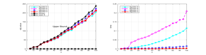
(a) Objective value and CPU time when $d=3$.

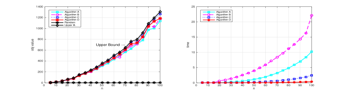
(b) Objective value and CPU time when $d=4$.

Figure 1: Comparisons of Algorithms A, B, C, and D for solving (2.3) where $\mathcal{A}$ is given by (4.15). $n$ varies from $5$ to $100$. Left panels: objective value $\mathcal{A}\mathbf{x}^{0}_{1}\cdots\mathbf{x}^{0}_{d}$ versus $n$; right panels: CPU time.

From the left panels, we observe that the objective values generated by Algorithms A, B, C, and D are similar, where Algorithm C performs better; Algorithm D performs the second when $d=4$, and it is comparable with Algorithm B when $d=3$; Algorithm A gives the worst results, which may be that Algorithm A does not explore the structure of the problem as much as possible. We also observe that the objective values of all the algorithms are quite close to the upper bound (4.16), which demonstrates the effectiveness of the proposed algorithms. In fact, the ratio of $\frac{\mathcal{A}\mathbf{x}^{0}_{1}\cdots\mathbf{x}^{0}_{d}}{v^{\rm ub}}$ is in $(0.7,1)$, which is far better than the approximation ratios presented in Sect. 3. This implies that at least for this kind of tensors, the approximation ratios might be independent of the size of the tensor. The value $\mathcal{A}\mathbf{x}^{\rm random}_{1}\cdots\mathbf{x}^{\rm random}_{d}$ is close to zero (the curve almost coincides with the $x$-axis). Concerning the computational time, Algorithms D is the most efficient one, confirming the theoretical results in Table 1. Algorithm C is the second efficient one. Algorithms A and B do not perform well compared with Algorithms C and D, although their computational complexity is similar in theory. The reason may be because the first two algorithms require for-loop operations, which is time-consuming in Matlab.

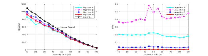
(a) Objective value and CPU time when $d=3$.

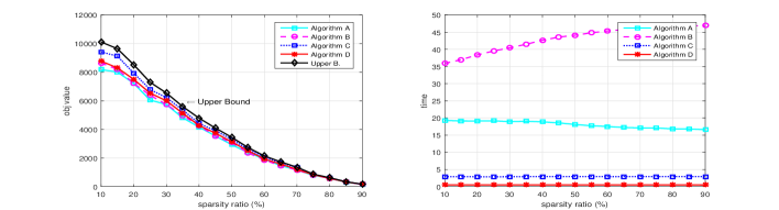
(b) Objective value and CPU time when $d=4$.

Figure 2: Comparisons of Algorithms A, B, C, and D for solving (2.3) with fixed $n$ and sparsity ratio varying from $10\%$ to $90\%$. Fig. 2(a): $\mathcal{A}\in\mathbb{R}^{100\times 100\times 100}$; Fig. 2(b): $\mathcal{A}\in\mathbb{R}^{100\times 100\times 100\times 100}$. Left panels: the objective values $\mathcal{A}\mathbf{x}^{0}_{1}\cdots\mathbf{x}^{0}_{d}$ versus sparsity ratio; right panels: CPU time.

We then consider fix $n=100$ and vary the sparsity ratio $sr$ from $10\%$ to $90\%$ of $\mathcal{A}$ in (4.15), and compare the performance of the four proposed algorithms. $r_{j}$ in (2.3) is set to $\lfloor(1-sr)n_{j}\rfloor$ correspondingly. The results of the objective values $\mathcal{A}\mathbf{x}^{0}_{1}\cdots\mathbf{x}^{0}_{d}$ together with the upper bound are depicted in the left panels of Fig. 2, from which we still observe that all the algorithms are close to the upper bound (4.16); among them, Algorithm C is still slightly better than the other three, followed by Algorithms B and D. The CPU time is plotted in the right panels of Fig. 2, which still shows that Algorithm D is the most efficient one. In fact, in average, Algorithm D is $5$ times faster than Algorithm C, which ranks the second, and is about $80$ times faster than Algorithm B, which is the slowest one.

Overall, comparing with Algorithms A and B that find the solutions fiber by fiber, or slide by slide, Algorithm C admits hierarchical structures that take the whole tensor into account, and so it can explore the structure of the data tensor better. This may be the reason why Algorithm C is better than Algorithms A and B in terms of the effectiveness. When compared with Algorithm D, Algorithm C computes each $\mathbf{x}^{0}_{j}$ “optimally” via SVD, while Algorithm D computes $\mathbf{x}^{0}_{j}$ “sub-optimally” but more efficiently; this explains why Algorithms C performs better than Algorithm D. Concerning the efficiency, Algorithms A and B require for-loop operations, which is known to be slow in Matlab. This leads to that although the algorithms have similar computational complexity in theory (Algorithms B and C), after implementation, their performances are quite different.

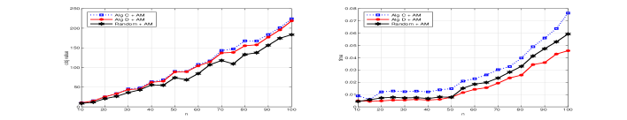
(a) Objective value and CPU time when $d=3$.

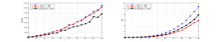
(b) Objective value and CPU time when $d=4$.

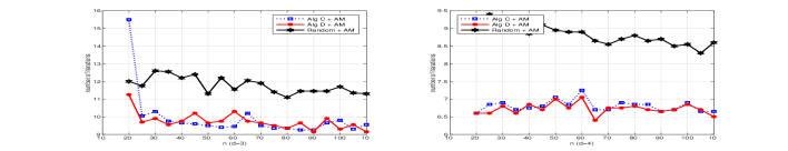
(c) Number of iterations. Left: $d=3$; right: $d=4$.

Figure 3: Performances of Alg. C + AM, Alg. D + AM and Random + AM for solving (2.3) where $\mathcal{A}$ is given by (4.15). $n$ varies from $10$ to $100$. The CPU time counts both that of approximation algorithms and AM.

Performance of approximation plus iterative algorithms

In this part, we first use approximation algorithms to generate $(\mathbf{x}^{0}_{1},\ldots,\mathbf{x}^{0}_{d})$, and then use it as an initializer for iterative algorithms. The goal is to see if approximation algorithms can help in improving the solution quality of iterative algorithms. The iterative algorithm used for solving problem (2.3) is simply an alternating maximization method (termed AM in the sequel) with the scheme

$$\boxed{{\rm(AM)}~{}~{}~{}~{}\mathbf{x}^{k+1}_{j}\in\arg\max\nolimits~{}{\mathcal{A}}{\mathbf{x}_{1}^{k+1}\cdots\mathbf{x}^{k+1}_{j-1}\mathbf{x}_{j}\mathbf{x}^{k}_{j+1}\cdots\mathbf{x}_{d}^{k}}~{}{\rm s.t.}~{}\left\|\mathbf{x}_{j}\right\|=1,\left\|\mathbf{x}_{j}\right\|_{0}\leq r_{j}}$$

for $j=1,\ldots,d$ and $k=1,2,\ldots$. The stopping criterion used for AM is $\max_{j}\{\left\|\mathbf{x}_{j}^{k+1}-\mathbf{x}_{j}^{k}\right\|\}\leq 10^{-5}$, or $k\geq 2000$. We employ Algorithms C and D in this part, and denote the approximation plus iterative algorithms as Alg. C + AM and D + AM in the sequel. As a baseline, we also evaluate AM initialized by randomly generated feasible point $(\mathbf{x}^{\rm random}_{1},\ldots,\mathbf{x}^{\rm random}_{d})$, which is generated the same as the previous part. This algorithm is denoted as Random + AM. The data tensors are also (4.15), where $50$ instances are randomly generated for each $n$. $r_{j}=\lfloor 0.3n_{j}\rfloor$. The objective values $\mathcal{A}\mathbf{x}^{\rm out}_{1}\cdots\mathbf{x}^{\rm out}_{d}$ and CPU time for third- and fourth-order tensors with $n$ varying from $10$ to $100$ are plotted in Fig. 3(a) and 3(b), where $(\mathbf{x}^{\rm out}_{1},\ldots,\mathbf{x}^{\rm out}_{d})$ is the output of AM. Here the CPU time counts both that of approximation algorithms and AM. Fig. 3(c) depicts the number of iterations of AM initialized by different strategies. Alg. C + AM is in blue, D + AM is in red, and Random + AM is in black.

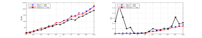
(a) $d=3$. Left: $\mathcal{A}\mathbf{x}^{\rm out}_{1}\cdots\mathbf{x}^{\rm out}_{d}$ versus $n$; right: CPU time versus $n$.

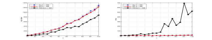
(b) $d=4$. Left: $\mathcal{A}\mathbf{x}^{\rm out}_{1}\cdots\mathbf{x}^{\rm out}_{d}$ versus $n$; right: CPU time versus $n$.

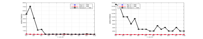
(c) Number of iterations versus $n$. Left: $d=3$; right: $d=4$.

Figure 4: Performances of Alg. C + AM ($\ell_{1}$), Alg. D + AM ($\ell_{1}$) and Random + AM ($\ell_{1}$) for solving (4.17) where $\mathcal{A}$ is given by (4.15). $n$ varies from $10$ to $100$.

In terms of objective value, we see from Fig. 3(a) and 3(b) that Alg. C + AM performs the best, while Alg. D + AM is slightly worse. Both of them are better than Random + AM, demonstrating that approximation algorithms can indeed help in improving the solution quality of iterative algorithms. Considering the efficiency, Alg. D + AM is the best among the three, followed by Random + AM. This further demonstrates the advantage of approximation algorithms. In fact, from Fig. 3(c), we can see that both Alg. C and D can help in reducing the number of iterations of AM. However, as we have observed in the previous part, Alg. C is more time-consuming than Alg. D, leading to that Alg. C + AM is the slowest one.

We also try to use Algorithms C and D to initialize AM for $\ell_{1}$ regularized model [1]:

$$\max~{}\left\langle\mathcal{A},\mathbf{x}_{1}\circ\cdots\circ\mathbf{x}_{d}\right\rangle-\sum^{d}_{j=1}\nolimits\rho_{j}\|\mathbf{x}_{j}\|_{1}~{}~{}{\rm s.t.}~{}~{}\|\mathbf{x}_{j}\|\leq 1,~{}1\leq j\leq d,$$ (4.17)

where $\rho_{j}=0.2$ is set in the experiment. The algorithms are denoted as Alg. C + AM ($\ell_{1}$), Alg. D + AM ($\ell_{1}$) and Random + AM ($\ell_{1}$). The results are plotted in Fig. 4, from which we observe similar results as those of Fig. 3; in particular, the efficiency of approximation algorithms plus AM ($\ell_{1}$) is significantly better than Random + AM ($\ell_{1}$), and their number of iterations is much more stable.

Overall, based on the observations of this part, compared with random initializations, iterative algorithms initialized by approximation solutions generated by approximation algorithms is superior both in terms of the solution quality and the running time.

Sparse tensor clustering

Tensor clustering aims to cluster matrix or tensor samples into their underlying groups: for $N$ samples $\mathcal{A}_{i}\in\mathbb{R}^{n_{1}\times\cdots\times n_{d}},i=1,\dots,N$ with $d\geq 2$ and given clusters $K\geq 2$, a clustering $\psi(\cdot)$ is defined as a mapping $\psi:\mathbb{R}^{n_{1}\times\dots\times n_{d}}\rightarrow\{1,\dots,K\}$. Several tensor methods have been proposed for tensor clustering; see, e.g., [26, 32, 31]. Usually, one can first perform a dimension reduction to the samples by means of (sparse) tensor decomposition, and then use classic methods such as $K$-means to the reduced samples for clustering. Here, we use a deflation method for tensor decomposition, including the proposed approximation algorithms as initialization procedures for AM as subroutines. The whole method for tensor clustering is presented in Algorithm STC, which has some similarities to [31, Algorithm 2]. We respectively use STC (A), STC (B), STC (C), STC (D) to distinguish AM involved in STC initialized by different approximation algorithms. We also denote STC (Random) as AM involved in STC with random initializations.

$$\noindent{\rm Algorithm}~{}(\psi(\mathcal{A}_{1}),\ldots,\psi(\mathcal{A}_{N}))={\rm sparse\_clustering}(\mathcal{A}_{1},\dots,\mathcal{A}_{N})$$ (STC) 1. Define $\mathcal{T}\in R^{n_{1}\times\cdots\times n_{d}\times N}$ with $\mathcal{T}(:,\ldots,:,i)=\mathcal{A}_{i}$, $i=1,\ldots,N$. 2. Apply a deflation method with rank-$R$ to $\mathcal{T}$, which employs Algorithm A, B, C, or D)+ AM to the residual tensors $\mathcal{T},\ldots,\mathcal{T}-\sum^{m}_{l=1}\alpha_{l}\mathbf{x}^{l}_{1}\circ\cdots\circ\mathbf{x}^{l}_{d+1},\ldots$, with resulting rank-1 terms $\mathbf{x}^{m}_{1}\circ\cdots\circ\mathbf{x}^{m}_{d+1}$ and weights $\alpha_{m}=(\mathcal{T}-\sum^{m-1}_{l=1}\alpha_{l}\mathbf{x}^{l}_{1}\cdots\mathbf{x}^{l}_{d+1})\mathbf{x}_{1}^{m}\cdots\mathbf{x}^{m}_{d+1}$, $m=1,\ldots,R$. Write $X_{j}:=[\mathbf{x}_{j}^{1},\ldots,\mathbf{x}_{j}^{R}]$, $j=1,\dots,d+1$ and $\boldsymbol{\alpha}:=[\alpha_{1},\dots,\alpha_{R}]^{\top}$. 3. Denote $\hat{X}_{d+1}=[\alpha_{1}\mathbf{x}_{d+1}^{1},\dots,\alpha_{R}\mathbf{x}_{d+1}^{R}]\in\mathbb{R}^{N\times R}$; here the $i$-th row of $\hat{X}_{d+1}$, denoted as $\hat{\mathbf{u}}_{i}$, is regarded as the reduced sample of $\mathcal{A}_{i}$. Apply $K$-means to clustering $\{\hat{\mathbf{u}}_{1},\dots,\hat{\mathbf{u}}_{N}\}\rightarrow\hat{\psi}(\hat{\mathbf{u}}_{j}),j=1,\dots,N$. 4. Return the cluster assignment of $\{\mathcal{A}_{1},\dots,\mathcal{A}_{N}\}$: $(\psi(\mathcal{A}_{1}),\ldots,\psi(\mathcal{A}_{N}))=(\hat{\psi}(\hat{\mathbf{u}}_{1}),\ldots,\hat{\psi}(\hat{\mathbf{u}}_{N}))$.

Denote $\psi_{0}$ as the true clustering mapping and let $|S|$ represent the cardinality of a set $S$. The following metric is commonly used to measure clustering performance [34]:

$${\rm cluster~{}err.}:=\tbinom{N}{2}^{-1}|\{i,j\}:(\psi(\mathcal{A}_{i})=\psi(\mathcal{A}_{j}))\not=(\psi_{0}(\mathcal{A}_{i})=\psi_{0}(\mathcal{A}_{j})),i<j|.$$

Synthetic Data

This experiment is similar to [31, Sect. 5.2]. Consider $N$ sparse matrix samples $\{A_{i}\in\mathbb{R}^{n_{1}\times n_{2}},i=1,\dots,N\}$ with $n_{1}=n_{2}=20$ as follows:

$$A_{1}=\dots=A_{\frac{N}{4}}~{}=\mu^{3}\cdot\begin{bmatrix}\Sigma&~{}&~{}\\ ~{}&-\Sigma&~{}\\ ~{}&~{}&\mathbf{0}\end{bmatrix},A_{\frac{N}{4}+1}=\dots=A_{\frac{N}{2}}~{}=\mu^{3}\cdot\begin{bmatrix}\Sigma&~{}&~{}\\ ~{}&\Sigma&~{}\\ ~{}&~{}&\mathbf{0}\end{bmatrix}$$

$$A_{\frac{N}{2}+1}=\dots=A_{\frac{3N}{4}}\hskip 0.85358pt=\mu^{3}\cdot\begin{bmatrix}-\Sigma&&\\ &\Sigma&\\ &&\mathbf{0}\end{bmatrix},A_{\frac{3N}{4}+1}=\dots=A_{N}\hskip 0.85358pt=\mu^{3}\cdot\begin{bmatrix}-\Sigma&&\\ &-\Sigma&\\ &&\mathbf{0}\end{bmatrix},$$

where $\Sigma=\mathbf{v}\mathbf{v}^{\top}\in\mathbb{R}^{4\times 4}$ with $\mathbf{v}=[1,-1,0.5,-0.5]^{\top}$, and $\mathbf{0}$ is a zero matrix of size $12\times 12$. We stack these samples into a third order tensor $\mathcal{T}\in\mathbb{R}^{n_{1}\times n_{2}\times N}$ with $\mathcal{T}(:,:,i)=A_{i}$. We apply STC (A), STC (B), STC (C), STC (D), and the vanilla $K$-means to the tensor $\mathcal{T}^{*}=\frac{\mathcal{T}}{||\mathcal{T}||_{F}}+\sigma\frac{\mathcal{E}}{||\mathcal{E}||_{F}}$ where $\mathcal{E}$ is a noisy tensor and $\sigma$ is the noise level. Here vanilla $K$-means stands for directly applying $K$-means to the vectorizations of $A_{i}$’s without tensor methods. We vary the sample number $N=\{20,40\}$ and noise level $\sigma=\{0.1,0.5,0.9\}$, and set $\mu=0.5$. To select parameters, we apply a similar Bayesian Information Criterion as [1]: For a set of parameter combinations defined as the cartesian product of the set $\mathfrak{R}$ of given ranks and the sets $\mathfrak{r}$ of tuning parameters, namely, $\mathfrak{R}\times\mathfrak{r}=\{(R,\boldsymbol{r})|R\in\mathfrak{R},\boldsymbol{r}\in\mathfrak{r}\}$, we select $(R^{*},{\boldsymbol{r}^{*}})=\arg\min_{\mathfrak{R}\times\mathfrak{r}}BIC(R,\boldsymbol{r})$ with

$$\small BIC(R,\boldsymbol{r}):=\log\left(\frac{\|\mathcal{T}-\sum_{l=1}^{R}\alpha_{l}\mathbf{x}^{l}_{1}\circ\dots\circ\mathbf{x}^{l}_{d+1}\|^{2}_{F}}{n_{1}\dots n_{d}N}\right)+\frac{\log(\prod^{d}_{j=1}n_{j}N)}{\prod^{d}_{j=1}n_{j}N}\sum_{l=1}^{R}\nolimits\sum^{d+1}_{j=1}\nolimits\|\mathbf{x}^{l}_{j}\|_{0},$$ (4.18)

where ${\alpha}_{l}$ and $\mathbf{x}^{l}_{j}$ are computed by Algorithm STC.

For tuning procedure, we set $\mathfrak{R}=\{4,6\}$ and $\mathfrak{r}=\{(7,7,N),(8,8,N)\}$. For the number $K$ of clusters, we employ the widely used evalclusters function in Matlab which evaluate each proposed number of clusters in a set $\{K_{1},\cdots,K_{m}\}$ and select the smallest number of clusters satisfying $Gap(K)\geq Gap(K+1)-SE(K+1),$ where $Gap(K)$ is the gap value for the clustering solution with $K$ clusters, and $SE(K+1)$ is the standard error of the clustering solution with $K+1$ clusters. The results are reported in Table 2 averaged over 50 instances in each case.

Table 2: Sparse tensor clustering via STC (A), STC (B), STC (C), STC (D) on synthetic data with different size $N$ and noise level $\sigma$. “cluster err.” represents the cluster error; “time” denotes the computational time (seconds).

		STC (A)		STC (B)		STC (C)		STC (D)		vanilla $K$-means
$N$	$\sigma$	cluster err.	time	cluster err.	time	cluster err.	time	cluster err.	time	cluster err.	time
20	0.1	0.00E+00	2.72E-01	0.00E+00	5.08E-01	0.00E+00	2.41E-01	0.00E+00	2.08E-01	9.37E-03	2.10E-03
20	0.5	3.05E-03	3.03E-01	6.53E-03	5.47E-01	0.00E+00	2.83E-01	0.00E+00	2.27E-01	2.53E-02	1.82E-03
20	0.9	1.22E-02	3.72E-01	6.53E-03	5.17E-01	1.22E-02	2.83E-01	3.05E-03	2.17E-01	5.21E-02	1.82E-03
40	0.1	0.00E+00	3.98E-01	0.00E+00	7.10E-01	0.00E+00	4.26E-01	0.00E+00	5.36E-01	3.10E-03	2.35E-03
40	0.5	3.18E-03	4.26E-01	6.28E-03	6.43E-01	0.00E+00	3.85E-01	2.97E-03	3.54E-01	2.26E-02	2.39E-03
40	0.9	3.21E-03	3.77E-01	9.08E-03	6.69E-01	3.10E-03	3.57E-01	3.18E-03	3.13E-01	5.33E-02	2.50E-03

Table 2 shows that the cluster error of STC with any approximation algorithm is smaller than that of the vanilla $K$-means in all cases and is even zero in some case when the noise level is not high, where the best one is STC (C), followed by STC (D). This shows the accuracy and robustness of our method. Considering the CPU time, among the four tensor methods, STC (D) is the most efficient one, followed by STC (C), while STC (B) needs more time than the other three. However, the computational time of tensor methods is not as good as that of the vectorized $K$-means, which is because of the increasing cost of the tuning procedure via (4.18) with a pre-specified set of parameter combinations.

Real data

We test the clustering performance of STC (D), STC (Random), and the vanilla $K$-means on Columbia Object Image Library COIL-20 [23] for image clustering. The data contains 20 objects viewed from varying angles and each image is of size $128\times 128$. The images are in grayscale, and the background of the objects is black, resulting in that the images can be seen as sparse matrices. In this experiment, we consider $K=\{5,6,7,8,9,10\}$ objects and pick up 36 images from each object for clustering, giving $\mathcal{T}\in\mathbb{R}^{128\times 128\times 36K}$. We still tune parameters of Algorithm STC via (4.18) and the evalclusters function in Matlab, and set $\mathfrak{R}=\{40,45\}$ and $\mathfrak{r}=\{(75,75,36K),(80,80,36K)\}$. The experiment has been repeated 20 times for each $K$, and the averaged results are shown in Table 3.

Table 3: Sparse tensor clustering via STC (D), STC (Random) and vanilla $K$-means on COIL-20 with different $K$.

	STC (D)		STC (Random)		vanilla $K$-means
$K$	cluster err.	time	cluster err.	time.	cluster err.	time
5	1.36E-01	1.62E+02	1.37E-01	1.70E+02	1.46E-01	2.21E-01
6	1.45E-01	1.90E+02	1.50E-01	2.02E+02	1.51E-01	2.79E-01
7	1.47E-01	2.23E+02	1.49E-01	2.46E+02	1.56E-01	3.53E-01
8	1.48E-01	2.63E+02	1.49E-01	2.84E+02	1.55E-01	3.91E-01
9	1.48E-01	2.93E+02	1.49E-01	2.97E+02	1.57E-01	4.40E-01
10	1.13E-01	3.09E+02	1.11E-01	3.43E+02	1.24E-01	5.39E-01

Table 3 shows that the cluster error of tensor methods is still better than that of the vanilla $K$-means, while STC (D) is slightly better than STC (Random). On the other hand, the computational time of STC (D) is less than that of STC (Random). However, it still needs more time than that of the vanilla $K$-means. There are two possible reasons for this phenomenon: first, it takes more time to tune parameters via (4.18); and second, our approach deals directly with data tensors instead of reshaping them into vectors, which preserves their intrinsic structures but naturally increases the computational complexity at the same time.

Overall, tensor methods armed with an approximation algorithm to generate good initializers show its ability to better exploring the data structure for clustering, and it would be interesting to further improve the efficiency.

5 Conclusions

Sparse tensor BR1Approx problem can be seen as a sparse generalization of the dense tensor BR1Approx problem and a higher-order extension of the matrix BR1Approx problem. In the literature, little attention was paid to approximation algorithms for sparse tensor BR1Approx. To fill this gap, four approximation algorithms were developed in this work, which are of low computational complexity, easily implemented, and all admit theoretical guaranteed approximation bounds. Some of the proposed algorithms and the associated aproximation bounds generalize their matrix or dense tensor counterparts, while Algorithm D, which is the most efficient one, is even new when reducing to the matrix or dense tensor cases. Numerical experiments on synthetic as well as real data showed the effectiveness and efficiency of the developed algorithms; in particular, we observed that compared with random initializations, our algorithms can improve the performance of iterative algorithms for solving the problem in question. Possible future work is to design algorithms with better approximation ratio; following [12, Theorem 4.3], we conjecture that the best ratio might be $O(\sqrt{\prod^{d}_{j=1}\frac{r_{j}}{n_{j}}}\cdot\sqrt{\prod^{d-2}_{j=1}\frac{\ln n_{j}}{n_{j}}})$. On the other hand, Qi defined and studied the best rank-1 approximation ratio of a tensor space [27]; it would be interesting to extend this notion to the sparse best rank-1 approximation setting and study its bounds.

References

• [1] G. I. Allen. Sparse higher-order principal components analysis. In International Conference on Machine Learning, pages 27–36, April 2012.
• [2] S. O. Chan, D. Papailliopoulos, and A. Rubinstein. On the approximability of sparse PCA. In Conference on Learning Theory, pages 623–646, 2016.
• [3] E. C. Chi and T. G. Kolda. On tensors, sparsity, and nonnegative factorizations. SIAM J. Matrix Anal. Appl., 33(4):1272–1299, 2012.
• [4] A. Cichocki. Era of big data processing: A new approach via tensor networks and tensor decompositions. arXiv preprint arXiv:1403.2048, 2014.
• [5] A. Cichocki, D. Mandic, L. De Lathauwer, G. Zhou, Q. Zhao, C. Caiafa, and H. A. Phan. Tensor decompositions for signal processing applications: From two-way to multiway component analysis. IEEE Signal Process. Mag., 32(2):145–163, 2015.
• [6] P. Comon. Tensors: a brief introduction. IEEE Signal Process. Mag., 31(3):44–53, 2014.
• [7] P. Comon and G. H. Golub. Tracking a few extreme singular values and vectors in signal processing. Proc. IEEE, 78(8):1327–1343, 1990.
• [8] P. Comon, X. Luciani, and A. De Almeida. Tensor decompositions, alternating least squares and other tales. J. Chemometr., 23(7-8):393–405, 2009.
• [9] A. d’Aspremont, L. El Ghaoui, M. I. Jordan, and G. R. G. Lanckriet. A direct formulation for sparse PCA using semidefinite programming. SIAM Rev., 49(3):434–448, January 2007.
• [10] L. De Lathauwer, B. De Moor, and J. Vandewalle. On the best rank-$1$ and rank-(${R}_{1},{R}_{2},\ldots,{R}_{n}$) approximation of higer-order tensors. SIAM J. Matrix Anal. Appl., 21:1324–1342, 2000.
• [11] A. d’Aspremont, F. Bach, and L. El Ghaoui. Approximation bounds for sparse principal component analysis. Math. Program., 148(1-2):89–110, 2014.
• [12] S. He, B. Jiang, Z. Li, and S. Zhang. Probability bounds for polynomial functions in random variables. Math. Oper. Res., 39(3):889–907, 2014.
• [13] S. He, Z. Li, and S. Zhang. Approximation algorithms for homogeneous polynomial optimization with quadratic constraints. Math. Program., Ser. B, 125:353–383, 2010.
• [14] C. J. Hillar and L.-H. Lim. Most tensor problems are NP-hard. J. ACM, 60(6):45:1–45:39, 2013.
• [15] B. Jiang, S. Ma, and S. Zhang. Tensor principal component analysis via convex optimization. Math. Program., Ser. A, 150:423–457, 2015.
• [16] T. G. Kolda and B. W. Bader. Tensor decompositions and applications. SIAM Rev., 51:455–500, 2009.
• [17] T. G. Kolda, B. W. Bader, and J. P. Kenny. Higher-order web link analysis using multilinear algebra. In Data Mining, Fifth IEEE International Conference on, pages 242–249. IEEE, 2005.
• [18] T. G. Kolda and J. R. Mayo. Shifted power method for computing tensor eigenpairs. SIAM J. Matrix Anal. Appl., 32(4):1095–1124, 2011.
• [19] L.-H. Lim. Singular values and eigenvalues of tensors: a variational approach. In Computational Advances in Multi-Sensor Adaptive Processing, 2005 1st IEEE International Workshop on, volume 1, pages 129–132, 2005.
• [20] R. Luss and M. Teboulle. Conditional gradient algorithms for rank-one matrix approximations with a sparsity constraint. SIAM Rev., 55(1):65–98, 2013.
• [21] O. H. Madrid-Padilla and J. Scott. Tensor decomposition with generalized lasso penalties. J. Comput. Graph. Stat., 26(3):537–546, 2017.
• [22] M. Magdon-Ismail. NP-hardness and inapproximability of sparse PCA. Infor. Process. Lett., 126:35–38, 2017.
• [23] S. A. Nene, S. K. Nayar, and H. Murase. Columbia object image library (COIL-20). Technical Report CUCS-005-96, 1996.
• [24] M. K.-P. Ng, X. Li, and Y. Ye. Multirank: co-ranking for objects and relations in multi-relational data. In Proceedings of the 17th ACM SIGKDD international conference on Knowledge discovery and data mining, pages 1217–1225, 2011.
• [25] J. Nie and L. Wang. Semidefinite relaxations for best rank-1 tensor approximations. SIAM J. Matrix Anal. Appl., 35(3):1155–1179, 2014.
• [26] E. E. Papalexakis, N. D. Sidiropoulos, and R. Bro. From K-means to higher-way co-clustering: Multilinear decomposition with sparse latent factors. IEEE Trans. Signal Process., 61(2):493–506, 2012.
• [27] L. Qi. The best rank-one approximation ratio of a tensor space. SIAM J. Matrix Anal. Appl., 32(2):430–442, 2011.
• [28] L. Qi, H. Chen, and Y. Chen. Tensor eigenvalues and their applications, volume 39. Springer, 2018.
• [29] N. D. Sidiropoulos, L. De Lathauwer, X. Fu, K. Huang, E. E. Papalexakis, and C. Faloutsos. Tensor decomposition for signal processing and machine learning. IEEE Trans. Signal Process., 65(13):3551–3582, 2017.
• [30] W. W. Sun and L. Li. STORE: sparse tensor response regression and neuroimaging analysis. J. Mach. Learn. Res., 18(1):4908–4944, 2017.
• [31] W. W. Sun and L. Li. Dynamic tensor clustering. J. Am. Stat. Assoc., 114(528):1894–1907, 2019.
• [32] W. W. Sun, J. Lu, H. Liu, and G. Cheng. Provable sparse tensor decomposition. J. Roy. Statist. Soc. Ser. B, 79(3):899–916, 2017.
• [33] N. Vervliet, O. Debals, L. Sorber, M. Van Barel, and L. De Lathauwer. Tensorlab 3.0, Mar. 2016. Available online.
• [34] J. Wang. Consistent selection of the number of clusters via crossvalidation. Biometrika, 97(4):893–904, 2010.
• [35] Y. Wang, M. Dong, and Y. Xu. A sparse rank-1 approximation algorithm for high-order tensors. Applied Math. Lett., 102:106140, 2020.
• [36] D. M. Witten, R. Tibshirani, and T. Hastie. A penalized matrix decomposition, with applications to sparse principal components and canonical correlation analysis. Biostat., 10(3):515–534, 2009.
• [37] Y. Yang, Y. Feng, X. Huang, and J. A. K. Suykens. Rank-1 tensor properties with applications to a class of tensor optimization problems. SIAM J. Optim., 26(1):171–196, 2016.
• [38] A. Zhang and R. Han. Optimal sparse singular value decomposition for high-dimensional high-order data. J. Am. Stat. Assoc., 114(528):1708–1725, 2019.
• [39] X. Zhang, L. Qi, and Y. Ye. The cubic spherical optimization problems. Math. Comput., 81(279):1513–1525, 2012.
• [40] H. Zou, T. Hastie, and R. Tibshirani. Sparse principal component analysis. J. Comput. Graph. Statist., 15(2):265–286, June 2006.