Graph Mixture Density Networks

Abstract

We introduce the Graph Mixture Density Networks, a new family of machine learning models that can fit multimodal output distributions conditioned on graphs of arbitrary topology. By combining ideas from mixture models and graph representation learning, we address a broader class of challenging conditional density estimation problems that rely on structured data. In this respect, we evaluate our method on a new benchmark application that leverages random graphs for stochastic epidemic simulations. We show a significant improvement in the likelihood of epidemic outcomes when taking into account both multimodality and structure. The empirical analysis is complemented by two real-world regression tasks showing the effectiveness of our approach in modeling the output prediction uncertainty. Graph Mixture Density Networks open appealing research opportunities in the study of structure-dependent phenomena that exhibit non-trivial conditional output distributions.

1 Introduction

Approximating the distribution of a target value $y$ conditioned on an input $x$ is at the core of supervised learning tasks. When trained using common losses such as Mean Square Error for regression or Cross-Entropy for classification, supervised methods are known to approximate the expected conditional distribution of the target given the input, that is, $\langle y|x\rangle$ (Bishop, 1994). This is standard practice when the target distribution is unimodal and slight variations in the target value are mostly due to random noise.

Still, when the target distribution of a regression problem is not unimodal, most machine learning methods fail to represent it correctly by predicting an averaged value. As a matter of fact, a multimodal target distribution associates more than one likely outcome with a given input sample, and in this case one usually talks about solving a conditional density estimation problem. To address this, the Mixture Density Network (MDN) (Bishop, 1994) was proposed to approximate arbitrarily complex conditional target distributions, and it finds application in robotics (Choi et al., 2018), epidemiology (Davis et al., 2020) and finance (Schittenkopf et al., 1998), to name a few. MDNs were designed for input data of vectorial nature, but often real-world problems deal with relational data where the structure substantially impacts the possible outcomes. For instance, this is especially true in epidemiology (Opuszko & Ruhland, 2013).

For more than twenty years, researchers have put great effort into the adaptive processing of graphs (see recent surveys of Bacciu et al. (2020b); Wu et al. (2020)). The goal is to infer the best representation of a structured sample for a given task via different neighborhood aggregation schemes, graph coarsening, and information propagation strategies. It is easy to find applications that benefit from the adaptive processing of structured data, such as drug design (Podda et al., 2020), classification in social networks (Yang et al., 2016), and natural language processing (Beck et al., 2018).

Our main contribution is the proposal of a hybrid approach to handle multimodal target distributions within machine learning methods for graphs, called Graph Mixture Density Network (GMDN). This model outputs a multimodal distribution, conditioned on an input graph, for either the whole structure or its entities. For instance, given an observable input graph $x$, GMDN is trained to approximate the (possibly multimodal) distribution associated with the target random variable $y$ via maximum likelihood estimation. The likelihood is the usual metric to be optimized for density estimation tasks (Nowicki & Snijders, 2001), and it tells us how well the model is fitting the empirical data distribution. Recall that, in general, it does not suffice to predict a single output value like in “standard” regression problems (Bishop, 1994) to solve this kind of tasks; for this reason, GMDN extends the capabilities of deep learning models for graphs whose output is restricted to unimodal distributions.

We test GMDN on a novel benchmark application introduced in this paper, comprising large epidemiological simulations where both structure and multimodality play an essential role in determining the outcome of an epidemic. Results show that GMDN produces a significantly improved likelihood. Then, we evaluate our model on two real-world chemical graph regression tasks to show how GMDN can better model the uncertainty in the output prediction, i.e., the model reveals that there might be more than one admissible chemical property value associated with a given input molecule representation.

2 Related Works

The problem of training a network to output a conditional multimodal distribution, i.e., a distribution with one or more modes, has been studied for 30 years. The Mixture of Experts (MoE) model (Jacobs et al., 1991; Jordan & Jacobs, 1994) is one of the first proposals that can achieve the goal, even though it was originally meant for a different purpose. The MoE consists of a multitude of neural networks, also called local experts, each being expected to solve a specific sub-task. In addition, an MoE uses a gating network to weigh the local experts’ contributions for each input. This way, the model selects the experts that are most likely to make the correct prediction. The overall MoE output is then the weighted combination of the local experts’ outputs; the reader is referred to Yuksel et al. (2012) and Masoudnia & Ebrahimpour (2014) for comprehensive surveys on this topic. Lastly, notice that the MoE imposes soft competition between the experts, but that may not be necessary when modeling the conditional distribution of the data.

The Mixture Density Network (MDN) of Bishop (1994), instead, reduces the computational burden of training an MoE while allowing the different experts, now called sub-networks, to cooperate. An MDN is similar to an MoE model, but it has subtle differences. First, the input is transformed into a hidden representation that is shared between simpler sub-networks, thus increasing the overall efficiency. Secondly, this representation is used to produce the gating weights as well as the parameters of the different output distributions. Hence, the initial transformation should encode all the information needed to solve the task into said representation. As the computational costs of processing the input grow, so does an MDN’s efficiency compared to an MoE. This is even more critical when the input is structured, such as a sequence or a graph, as it requires more resources to be processed.

In terms of applications, MDNs have been recently applied to epidemic simulation prediction (Davis et al., 2020). The goal is to predict the multimodal distribution of the total number of infected cases under a compartmental model such as the stochastic Susceptible-Infectious-Recovered (SIR) model (Kermack & McKendrick, 1927). In the paper, the authors show that, given samples of SIR simulations with different infectivity and recovery parameters, the MDN could approximate the conditioned output distribution using a mixture of binomials. This result is a remarkable step in approximating way more complex compartmental models in a fraction of the time originally required, similarly to what has been done, for example, in material sciences (Pilania et al., 2013). However, the work of Davis et al. (2020) makes the strong assumption that the infected network is a complete graph. In fact, as stated in (Opuszko & Ruhland, 2013), arbitrary social interactions in the network play a fundamental role in the spreading of a disease. As such, predictive models should be able to take them into account.

The automatic and adaptive extraction of relational information from graph-structured data is another long-standing research topic (Sperduti & Starita, 1997; Frasconi et al., 1998; Micheli, 2009; Scarselli et al., 2009) that has found widespread application in social sciences, chemistry, and bioinformatics. In the recent past, graph kernels (Ralaivola et al., 2005; Vishwanathan et al., 2010) were the main methodology to process structural information; while still effective and powerful, the drawback of graph kernels is the computational costs required to compute similarity scores between pairs of graphs. Nowadays, the ability to efficiently process graphs of arbitrary topology is made possible by a family of models called Deep Graph Networks (DGNs). A DGN stacks graph convolutional layers, which aggregate each node’s neighboring states, to propagate information across the graph. The number of layers reflects the amount of contextual information that propagates (Micheli, 2009), very much alike to receptive fields of convolutional neural networks (LeCun et al., 1995). There is an increasingly growing literature on the topic which is not covered in this work, so we refer the reader to recent introductory texts and surveys (Bronstein et al., 2017; Battaglia et al., 2018; Bacciu et al., 2020b; Wu et al., 2020).

For the above reasons, we propose the Graph Mixture Density Networks to combine the benefits of MDNs and DGNs. To the best of our knowledge, this is the first DGN that can learn multimodal output distributions conditioned on arbitrary input graphs.

Figure 1: From a high-level perspective, a DGN transforms each node $v$ of the input graph $g$ into a hidden representation $\mathbf{h}_{v}$ that encodes the structural information surrounding that node. Then, in this work, a subsequent transformation $\Phi_{Q}$ generates the mixing probability vector $Q_{g}\in[0,1]^{C}$ that combines the $C$ different distributions produced by the sub-networks $\Phi_{1},\dots,\Phi_{C}$. Similarly to MDNs, the input’s first transformation is shared between the sub-networks. For example, suppose we were to predict the outcome of a stochastic SIR simulation. In that case, orange round nodes might represent initially infected entities in a network of size $n$, and $\beta,\gamma,R0$ would be simulation-specific node attributes.

3 Graph Mixture Density Networks

A graph is defined as a tuple $g=(\mathcal{V}_{g},\mathcal{E}_{g},\mathcal{X}_{g})$ where $\mathcal{V}_{g}$ is the set of nodes representing entities, $\mathcal{E}_{g}$ is the set of edges that connect pairs of nodes, and $\mathcal{X}_{g}$ denotes the (optional) node attributes. For the purpose of this work, we do not use edge attributes even though the approach can be straightforwardly extended to consider them.

The task under consideration is a supervised conditional density estimation (CDE) problem. We aim to learn the conditional distribution $P(y_{g}|g)$, with $y_{g}$ being the continuous target label(s) associated with an input graph $g$ in the dataset $\mathcal{D}$. We assume the target distribution to be multimodal, and as such it cannot be well modeled by current DGNs due to the aforementioned averaging effects. Therefore, we borrow ideas from the Mixture Density Network (Bishop, 1994) and extend the family of deep graph networks with multimodal output capabilities.

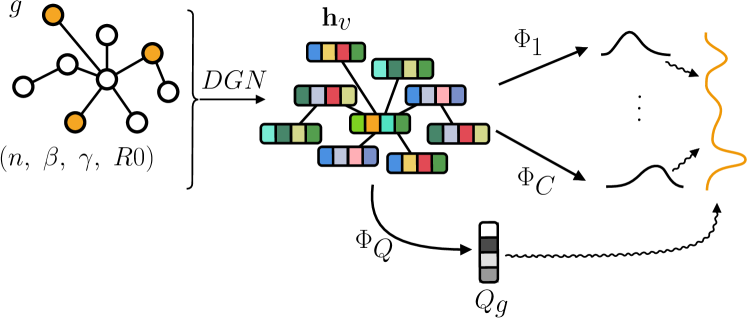
From a high-level perspective, we seek a DGN that performs an isomorphic transduction (Frasconi et al., 1998) to obtain node representations $\mathbf{h}_{\mathcal{V}_{g}}=\{\mathbf{h}_{v}\in\mathbb{R}^{d},d\in\mathbb{N},\ \forall v\in g\}$ as well as a set of “mixing weights” $Q_{g}\in[0,1]^{C}$ that sum to 1, where $C$ is the number of unimodal output distributions we want to mix. Given $\mathbf{h}_{\mathcal{V}_{g}}$, we then apply $C$ different sub-networks $\Phi_{1},\dots,\Phi_{C}$ that produce the parameters $\theta_{1},\dots,\theta_{C}$ of $C$ output distributions, respectively.

In principle, we can mix distributions from different families, but this poses several issues, such as their choice and how many of them to use for each family. In light of this, we stick to a single family for simplicity of exposition. Finally, combining the $C$ unimodal output distributions with the mixing weights $Q_{g}$ produces a multimodal output distribution. We sketch the overall process in Figure 1 for the specific case of epidemic simulations.

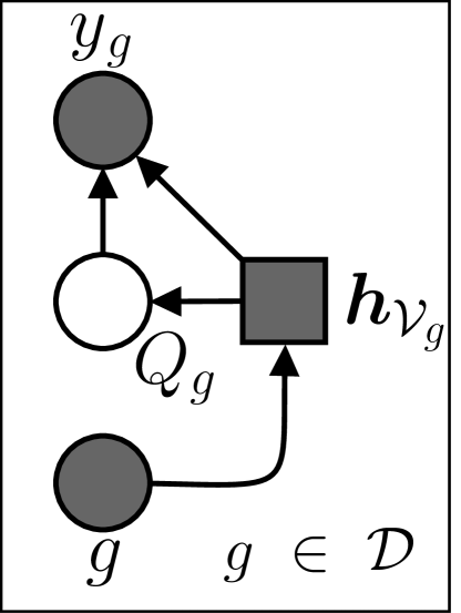
More formally, we learn the conditional distribution $P(y_{g}|g)$ using the Bayesian network of Figure 2. Here, round white (dark) nodes represent unobserved (observed) random variables, and larger squares indicate deterministic outputs. The mixing weights $Q_{g}$ are modeled as a categorical distribution with $C$ possible states.

We solve the CDE problem by maximum likelihood estimation (MLE). The likelihood, i.e., $P(y|g)$, is the usual quantity to be maximized. It reflects the probability that an output $y$ is generated from a graph $g$. Given an hypotheses space $\mathcal{H}$, we seek the MLE hypothesis:

$$h_{MLE}=arg\max_{h\in\mathcal{H}}P(\mathcal{D}|h)=$$

$$=arg\max_{h\in\mathcal{H}}\prod_{g\in\mathcal{D}}\sum_{i=1}^{C}P(y_{g}|Q^{i}_{g},g)P(Q^{i}_{g}|g),$$ (1)

where we introduced the latent variable $Q_{g}$ via marginalization whose i-th component is $Q_{g}^{i}$. In particular, we will model the distributions of Equation 1 by means of deep graph networks, which allow great flexibility with respect to the input structure and invariance to graph automorphism. This way, we are able to approximate probabilities that are conditioned on a variable number of graph nodes and edges.

Figure 2: The model can be graphically represented as a Bayesian network where round white (dark) nodes are unobserved (observed) random variables. For each graph $g$ in the dataset $\mathcal{D}$, we introduce the latent variable $Q_{g}$ via marginalization. This allows us to break the computation of $P(y_{g}|g)$ in two steps. The first step encodes the graph information into deterministic node states $\mathbf{h}_{\mathcal{V}_{g}}$ and produces the posterior distribution $P(Q_{g}|g)$. In the second and final step, we output the emission distributions $P(y_{g}|Q_{g}=i,g),i=1,\dots,C$. The result is a mixture model conditioned on the input structure.

As mentioned earlier, a deep graph network encodes the input graph into node representations $\mathbf{h}_{\mathcal{V}_{g}}$. Generally speaking, this encoder stacks multiple layers of graph convolutions to generate intermediate node states $\mathbf{h}_{v}^{\ell}$ at each layer $\ell=1,\dots,L$:

$$\mathbf{h}_{v}^{\ell+1}=\phi^{\ell+1}\Big{(}\mathbf{h}_{v}^{\ell},\ \Psi(\{\psi^{\ell+1}(\mathbf{h}_{u}^{\ell})\mid u\in\mathcal{N}_{v}\})\Big{)},$$ (2)

where $\phi$ and $\psi$ are (possibly non-linear) functions, and $\Psi$ is a permutation invariant function applied to node $v$’s neighborhood $\mathcal{N}_{v}$. Usually, the final node representation $\mathbf{h}_{v}$ is given by $\mathbf{h}^{L}_{v}$ or, alternatively, by the concatenation of all intermediate states. The convolution of the Graph Isomorphism Network (GIN) (Xu et al., 2019) is a particular instance of Equation 2 that we will use in our experiments to compute graph-related probabilities, as these need to be permutation invariant with respect to the node ordering.

In graph-prediction, representations $\boldsymbol{h}_{\mathcal{V}_{g}}$ have to be further aggregated with another permutation invariant function $\Psi_{g}$

$$\mathbf{h}_{g}=r_{g}(\mathbf{h}_{\mathcal{V}_{g}})=\Psi_{g}\Big{(}\{f_{r}(\mathbf{h}_{v})\mid v\in\mathcal{V}_{g}\}\Big{)},$$ (3)

where $f_{r}$ could be a linear model or a Multi-Layer Perceptron. Equation 3 is often referred to as the “readout” phase. Instead, the mixing weights can be computed using a readout $r^{Q}_{g}$ as follows:

$$P(Q_{g}|g)=\sigma(r^{Q}_{g}(\mathbf{h}_{\mathcal{V}_{g}})),$$ (4)

where $\sigma$ is the softmax function over the components of the aggregated vector.

To learn the emission $P(y_{g}|Q^{i}_{g},g),\ i=1,\dots,C$, we have to implement a sub-network $\Phi_{i}$ that outputs the parameters of the chosen distribution. For instance, if the distribution is a multivariate Gaussian we have

$$\boldsymbol{\mu_{i}},\boldsymbol{\Sigma_{i}}=\Phi_{i}(\mathbf{h}_{g})=f_{i}(r^{i}_{g}(\mathbf{h}_{\mathcal{V}_{g}})),$$ (5)

with $f_{i}$ being defined as $f_{r}$ above. Note that node-prediction tasks do not need a global readout phase, so Equations 4 and 5 are directly applied to $\mathbf{h}_{v}\ \forall v\in\mathcal{V}_{g}$.

Differently from the Mixture of Experts, which would require a new DGN encoder for each output distribution $i$, we follow the Mixture Density Network approach and share $\mathbf{h}_{\mathcal{V}_{g}}$ between the sub-networks. This form of weight sharing reduces the number of parameters and pushes the model to extract all the relevant structural information into $\mathbf{h}_{\mathcal{V}_{g}}$. Furthermore, using multiple DGN encoders can become computationally intractable for large datasets.

Training.

We train the Graph Mixture Density Network using the Expectation-Maximization (EM) framework (Dempster et al., 1977) for MLE estimation. We choose EM for the local convergence guaranteees that it offers with respect to other optimizers, and since its effectiveness has already been proved on probabilistic graph models (Bacciu et al., 2018, 2020a). Indeed, by introducing the usual indicator variable $z^{g}_{i}\in\mathcal{Z}$, which is one when graph $g$ is in latent state $i$, we can compute the lower bound of the log-likelihood as in standard mixture models (Jordan & Jacobs, 1994; Corduneanu & Bishop, 2001):

$$\mathbb{E}_{\mathcal{Z}|\mathcal{D}}[\log\mathcal{L}_{c}(h|\mathcal{D})]=$$

$$=\sum_{g\in\mathcal{D}}\sum_{i=1}^{C}E[z_{i}^{g}|\mathcal{D}]\log\Big{(}P(y_{g}|Q^{i}_{g},g)P(Q_{g}|g)\Big{)}$$ (6)

where $\log\mathcal{L}_{c}(h|\mathcal{D})$ is the complete log likelihood.

The E-step of the EM algorithm can be performed analytically by computing the posterior probability of the indicator variables:

$$E[z_{i}^{g}|\mathcal{D}]=P(z^{g}_{i}=1|g)=\frac{1}{Z}P(y_{g}|Q^{i}_{g},g)P(Q_{g}|g)$$ (7)

where $Z$ is the usual normalization term obtained via straightforward marginalization. On the other hand, we do not have closed-form solutions for the M-step because of the non-linear functions used. Hence, we perform the M-step using gradient ascent to maximize Equation 6. The resulting algorithm is known as Generalized EM (GEM) (Dempster et al., 1977). GEM still guarantees convergence to a local minimum if each optimization step improves Equation 6. Finally, we introduce an optional Dirichlet regularizer $\pi$ with hyper-parameter $\boldsymbol{\alpha}=(\alpha_{1},\dots,\alpha_{C})$ on the distribution $P(Q_{g}|g)$. The prior distribution serves to prevent the posterior probability mass of the from collapsing onto a single state. This is a well-known problem that has been addressed in the literature through specific constraints (Eigen et al., 2013) or entropic regularization terms (Pereyra et al., 2017). Here, the objective to be maximized becomes

$$\underbrace{\mathbb{E}_{\mathcal{Z}|\mathcal{D}}[\log\mathcal{L}_{c}(h|\mathcal{D})]}_{\text{original objective}}+\underbrace{\sum_{g\in\mathcal{D}}\log\pi(Q_{g}|\boldsymbol{\alpha})}_{\text{Dirichlet regularizer}},$$ (8)

where we note that $\boldsymbol{\alpha}=\boldsymbol{1}^{C}$ corresponds to a uniform prior, i.e., no regularization. To conclude, maximizing Equation 8 still preserves the convergence guarantees of GEM if the original objective increases at each step.

4 Experiments

This section thoroughly describes the datasets, experiments, evaluation process and hyper-parameters used. This work aims at showing that GMDN can fit multimodal distributions conditioned on a graph better than using MDNs or DGNs individually. To do so, we publicly release large datasets of stochastic SIR simulations whose results depend on the underlying network, rather than assuming uniformly distributed connections as in Davis et al. (2020). We generate random graphs using the Barabasi-Albert (BA) (Barabási & Albert, 1999) and Erdos-Renyi (ER) (Bollobás & Béla, 2001) models. While ER graphs do not preserve social networks’ properties, here we are interested in the emergence of multimodal outcome distributions rather than biological plausibility. That said, future investigation will cover more realistic cases, for instance using the Block Two-Level Erdos–Renyi model (Seshadhri et al., 2012). We expect GMDN to perform better because it takes both multimodality and structure into account during training. Moreover, we analyze whether training on a particular family of graphs exhibits transfer properties; if that is the case, then the model has learned how to make informed predictions about different (let alone completely new) structures. At last, we apply the model on two molecular graph regression benchmarks to analyze the performances of GMDN on real-world data.

Figure 3: Given a single network and specific choices for $R0=\beta/\gamma$, the repeated simulation of the stochastic SIR model is known to produce different outcomes. Here we plot the outcome distributions of 1000 SIR simulations on an Erdos-Renyi network of size 200. We follow Davis et al. (2020) and sample $\beta$ and $\gamma$ uniformly, rather than their ratio, because higher ratios correspond to less interesting behaviors, i.e., the distribution becomes unimodal. Depending on the input structure, the distribution of the total infected cases may be multimodal or not, and the GMDN should recognize this phenomenon. In our simulations, larger networks exhibited less multimodality; hence, without loss of generality, we focus on larger datasets of smaller graphs.

Datasets.

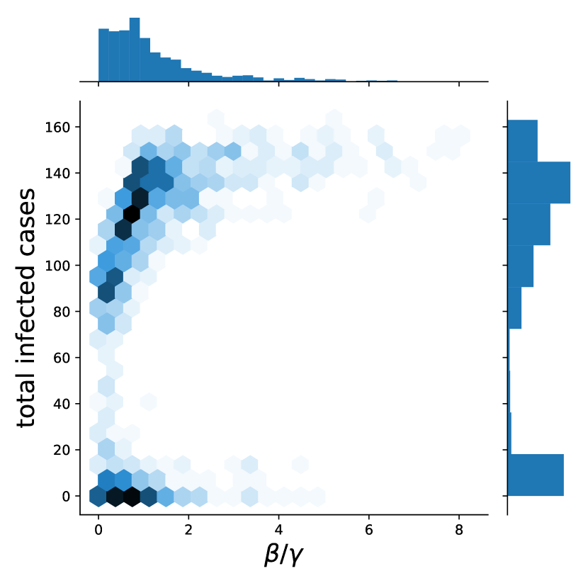
We simulated the well-known stochastic SIR epidemiological model on Barabasi-Albert graphs of size 100 (BA-100), generating 100 random graphs for different connectivity values (2, 5, 10 and 20). Borrowing ideas from Davis et al. (2020), for each configuration, we run 100 simulations for each different initial infection probability (1%, 5%, 10%) sampling the infectivity parameter $\beta$ from $[0,1]$ and the recovery parameter $\gamma$ from $[0.1,1]$. We also carry out simulations for Erdos-Renyi graphs (ER-100), this time with connectivity parameters 0.01, 0.05, 0.1, and 0.2. The resulting total number of simulations (i.e., samples) in each dataset is 120.000, and the goal is to predict the distribution of the total infected cases at the end of a simulation. Node features consist of $\beta$, $\gamma$, their ratio $R0=\beta/\gamma$, a constant value $1$, and a binary value that indicates whether that node is infected or not at the beginning of the simulation. Moreover, to test the transfer learning capabilities of GMDN on graphs with different structural properties (according to the chosen random graph model), we constructed six additional simulation datasets where graphs have different sizes, i.e., from 50 to 500. An example of simulation results is summarized in Figure 3; we observe that the outcome distribution of repeated simulations on a single graph leads to a multimodal distribution, in accord with (Opuszko & Ruhland, 2013). Therefore, in principle, being able to accurately and efficiently predict the outcome distribution of a (possibly complex) epidemiological model can significantly impact the preparations for an incumbent sanitary emergency.

When dealing with graph regression tasks, especially in the chemical domain, we usually do not expect such a conspicuous emergence of multimodality in the output distribution. Indeed, the properties of each molecule are assumed to be regulated by natural laws, but the information we possess about the input representation may be incomplete and/or noisy. Similarly, the way the model processes the input has an impact on the overall uncertainty; for instance, disregarding bond information makes graphs appear isomorphic to the model while they are indeed not so. As such, knowing the confidence of a trained regressor for a specific outcome becomes invaluable to better understand the data, the model behavior, and, ultimately, to determine the trust we place in each prediction. Therefore, we will evaluate our model on the large chemical benchmarks alchemy_full (Chen et al., 2019) and ZINC_full (Irwin et al., 2012; Bresson & Laurent, 2019) made of 202579 and 249456 molecules, respectively. The task of both datasets is the prediction of continuous chemical properties (12 for the former and 1 for the latter) associated with each molecule representation (9 and 28 node features, respectively). As in Chen et al. (2019), the GIN convolution used only considers the existence of a bond between atoms. In the considered datasets, this gives rise to isomorphic representations of different molecules when bond types or 3D coordinates are not considered (or ignored by the model). The same phenomena, in different contexts and forms, can occur whenever the original data or its choice of representation lack part of the information to solve a task.

Evaluation Setup.

We assess the performance of different models using a holdout strategy for all datasets ($80\%/10\%/10\%$ split). Given the size of the datasets, we believe that a simple holdout is sufficient to assess the performances of the different models considered. To make the evaluation even more robust for the epidemic datasets, different simulations about the same graph cannot appear in both training and test splits. The metric of interest is the log-likelihood of the data ($\log\mathcal{L}$), which captures how well we can fit the target distribution and the model’s uncertainty with respect to a particular output value. We also report the Mean Average Error (MAE) on the real-world benchmarks for completeness. However, the MAE does not reflect the model’s uncertainty about the output, as we will show.

We perform model selection via grid search for all the models presented. For each of them, we select the best configuration on the validation set using early stopping with patience (Prechelt, 1998). Then, to avoid an unlucky random initialization of the chosen configuration, we average the model’s performance on the unseen test set over ten final training runs. Similarly to the model selection phase, in these final training runs we use early stopping on a validation set extracted from the training set (10% of the training data).

Baselines and hyper-parameters.

We compare GMDN against four different baselines. First, RAND predicts the uniform probability over the finite set of possible outcomes, thus providing the threshold log-likelihood score above which predictions are useful. Instead, HIST computes the normalized frequency histogram of the target values given the training data, which is then converted into a discrete probability. While on epidemic simulations we can use the graph’s size as the number of histogram bins to use, on the chemical benchmarks this number must be treated as a hyper-parameter and manually cross-validated against the validation set. HIST is used to test whether multimodality is useful when a model does not take the structure into account. Finally, we have MDN and DGN, which are, in a sense, ablated versions of GMDN. Indeed, MDN ignores the input structure, whereas DGN cannot model multimodality. Neural models are trained to output unimodal (DGN) or multimodal (MDN, GMDN) binomial distributions for the epidemic simulation datasets and isotropic Gaussians for the chemical ones. The sub-networks $\Phi_{i}$ are linear models, and the graph convolutional layer is adapted from Xu et al. (2019). We conclude the section by listing the hyper-parameters tried for each model:

• MDN: $C$ $\in$ {2,3,5}, hidden units per convolution $\in$ {64}, neighborhood aggregation $\in$ {sum}, graph readout $\in$ {sum, mean}, $\boldsymbol{\alpha}$ $\in$ {$\boldsymbol{1}^{C}$, $\boldsymbol{1.05}^{C}$}, epochs $\in$ {2500}, $\Phi_{i}$ $\in$ {Linear model}, Adam Optimizer with learning rate $\in$ {0.0001}, full batch, patience $\in$ {30}.

• GMDN: $C$ $\in$ {3,5}, graph convolutional layers $\in$ {2,5,7}, hidden units per convolution $\in$ {64}, neighborhood aggregation $\in$ {sum}, graph readout $\in$ {sum, mean}, $\boldsymbol{\alpha}$ $\in$ {$\boldsymbol{1}^{C}$, $\boldsymbol{1.05}^{C}$}, epochs $\in$ {2500}, $\Phi_{i}$ $\in$ {Linear model}, Adam Optimizer with learning rate $\in$ {0.0001}, full batch, patience $\in$ {30}.

• DGN: same as GMDN but $C$ $\in$ {$1$} (that is, it outputs a unimodal distribution).

Note that we kept the maximum number of epochs intentionally high as we use early stopping to halt training.Also, the results of the experiments hold regardless of the DGN variant used, given the fact that DGNs output a single value rather than a complex distribution. In other words, we compare families of models rather than specific architectures.

5 Results and Discussion

Model	BA-100	ER-100	Structure	Multimodal
RAND	-4.60	-4.60	✗	✗
HIST	-1.16	-2.32	✗	✓
MDN	-1.17(.05)	-2.54(.07)	✗	✓
DGN	-0.90(.35)	-1.96(.16)	✓	✗
GMDN	-0.67(.02)	-1.56(.04)	✓	✓

Table 1: Results on BA-100 e ER-100 (12.000 test samples each). A higher log-likelihood corresponds to better performances. GMDN improves the performance on both tasks, showing the advantages of that taking into account both multimodality and structure. Neural models’ results are averaged over 10 runs, and standard deviation is reported in brackets.

Figure 4: The trend of the mixing weights (left) and binomial coefficient (right) for each one of five sub-networks is shown on 100 ER-100 graphs. We vary the ratio between infection and recovery rate to inspect the behavior of the GMDN. Here, we see that sub-network 4 can greatly change the binomial output distribution in a way that depends on the input graph.

This section discusses our experimental findings. We start from the main empirical study on epidemic simulations, which include CDE results and transferability of the learned knowledge. Then, we report results obtained on the real-world chemical tasks, highlighting the importance of capturing a model’s uncertainty about the output predictions.

Epidemic Simulation Results

We begin by analyzing the results obtained on BA-100 and ER-100 in Table 1. We notice that GMDN has better test log-likelihoods than the other baselines, with larger performance gains on ER-100. Being GMDN the only model that considers both structure and multimodality, such an improvement was expected. However, it is particularly interesting that HIST has a better log-likelihood than MDN on both tasks. By combining this fact with the results of DGN, we come to two conclusions. First, the structural information seems to be the primary factor of performance improvement; this should not come as a surprise since the way an epidemic develops depends on how the network is organized (despite we are not aiming for biological plausibility). Secondly, none of the baselines can get close enough to GMDN on ER-100, indicating that this task is harder to solve by looking individually at structure or multimodality. In this sense, BA-100 might be considered an easier task than ER-100, and this is plausible because emergence of multimodality on the former task seems slightly less pronounced in the SIR simulations. For completeness, we also tested an intermediate baseline where DGN is trained with L1 loss followed by MDN on the graph embeddings. Results displayed a $\log\mathcal{L}\approx-16$ on both datasets, probably because the DGN creates similar graph embeddings for different distributions with the same mean, with consequent severe loss of information.

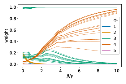
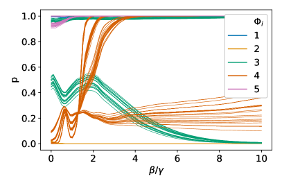
Similarly to what has been done in Bishop (1994) and Davis et al. (2020), we analyze how the mixing weights and the distribution parameters vary on a particular GMDN instance. We use $C$=5 and track the behavior of each sub-network for 100 different ER-100 graphs. Figure 4 shows the trend of the mixing weights (left) and of the binomial parameters $p$ (right) for different values of the ratio $R0=\beta/\gamma$. We immediately see that many of the sub-networks are “shut down” as the ratio grows. In particular, sub-networks 3 and 4 are the ones that control GMDN’s output distribution the most, though for high values of R0 only one sub-network suffices. These observations are concordant with the behavior of Figure 3: when the infectivity rate is much higher than the recovery rate, the target distribution becomes unimodal. The analysis of the binomial parameter for sub-network 4 provides another interesting insight. We notice that, depending on the input graph, the sub-network leads to two possible outcomes: the outbreak of the disease or a partial infection of the network. Note that this is a behavior that GMDN can model whereas the classical MDN cannot.

Figure 5: Output distributions of MDN, DGN, and GMDN on an ER graph of size 100. As we can see, the GMDN can provide a rich multimodal distribution conditioned on the structure close to that generated by SIR simulations (blue histogram).

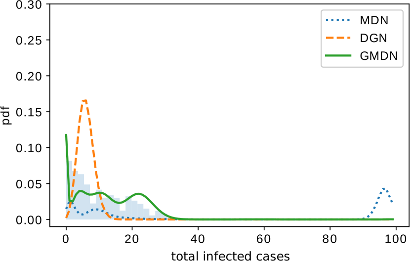
To provide further evidence about the benefits of the proposed model, Figure 5 shows the output distributions of MDN, DGN and GMDN for a given sample of the ER-100 dataset. We also plot the result of SIR simulations on that sample as a blue histogram (ground truth). Some observations can be made. First, the MDN places the output probability mass at both sides of the plot. This choice is understandable considering the lack of knowledge about the underlying structure (see also Table 1) and the fact that likely output values tend to be polarized at the extremes (see e.g., Figure 3). Secondly, the DGN can process the structure but cannot model more than one outcome. Therefore, and coherently with Bishop (1994) for vectorial data, the DGN unique mode lies in between those of GMDN that account for the majority of GMDN probability mass. In contrast, GMDN produces a multimodal and structure-aware distribution that closely follows the ground truth.

Figure 6: Transfer learning effect of the trained GMDNs are shown as blue dots and orange squares. Higher scores are better. GMDN trained on ER-100 exhibits better transfer on larger BA-datasets, which might be explained by the difficulty of the source task.

Transfer Results

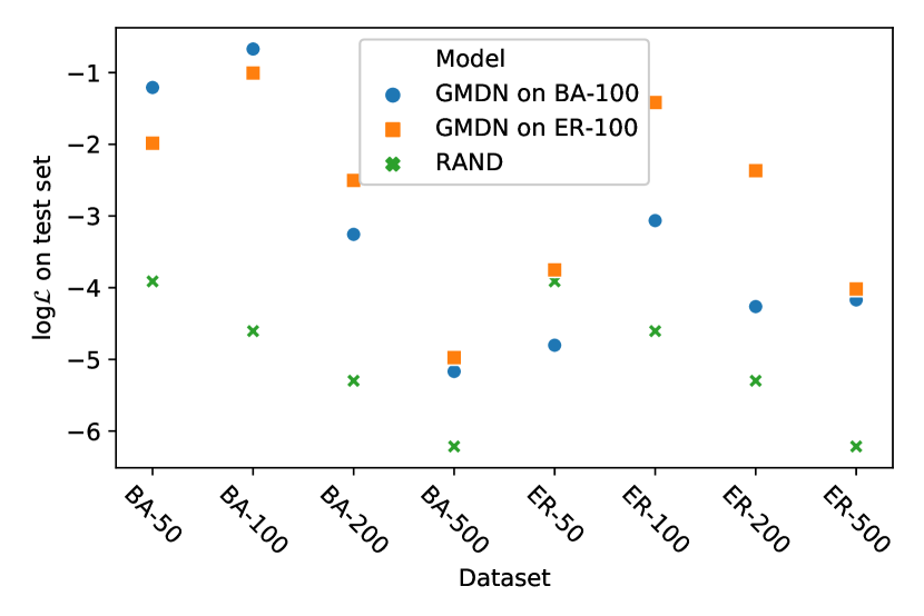
To tell whether GMDN can transfer knowledge to a random graph of different size and/or family (i.e., with different structural properties), we evaluate the trained models on the six additional datasets described in Section 4. Results are shown in Figure 6, where the RAND score acts as the reference baseline. The general trend is that the GMDN trained on ER-100 has better performances than its counterpart trained on BA-100; this is true for all ER datasets, BA-200 and BA-500. This observation suggests that training on ER-100, which we assumed to be a “harder” task than BA-100 as discussed above, allows the model to better learn the dynamics of SIR and transfer them to completely different graphs. Since the structural properties of the random graphs vary across the datasets, obtaining a transfer effect is therefore not an obvious task.

Model	alchemy_full		ZINC_full
	$\log\mathcal{L}$	MAE	$\log\mathcal{L}$	MAE
RAND	-27.12	-	-4.20	-
HIST	-21.91	-	-1.28	-
MDN	-1.36(.90)	0.62(.01)	-1.14(.01)	0.67(.00)
DGN	-7.19(1.3)	0.62(.01)	-0.90(.10)	0.49(.03)
GMDN	-0.57(1.4)	0.61(.02)	-0.75(.10)	0.49(.04)

Table 2: Results on the chemical tasks show how GMDN consistently reaches better log-likelihood values than the baselines. We also report the MAE as secondary metric for future reference, using the weighted mean of the sub-networks as the prediction (see Bishop (1994) for alternatives). Clearly, the MAE does not reflect the amount of uncertainty in a model’s prediction, whereas the log-likelihood is the natural metric for that matter. Results are averaged over 10 training runs with standard deviation in brackets.

Figure 7: We illustrate the output distributions on the first component, i.e., dipole moment, of an alchemy_full graph. As noted in the text, DGN places high confidence in between the two modes of GMDN. On the contrary, GMDN is able to express uncertainty about the possible output values (vertical lines) associated with isomorphic graphs, which can be found if 3D attributes are not considered. The existence of the two modes suggests that 3D attributes are nonetheless ignored by the three models. See the discussion in Section 4 for a more in-depth explanation of the phenomenon.

Chemical Benchmarks

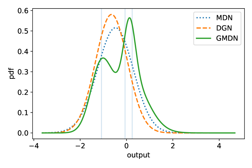
We conclude this section with results on the real-world chemical benchmarks, which are summarized in Table 2. We observe a log-likelihood trend similar to that in Table 1, with the notable difference that DGN performs much worse than MDN on alchemy_full. Following the discussion in Section 4, we evaluate how models deal with the uncertainty in the prediction by analyzing one of the output components of alchemy_full. Figure 7 shows such an example for the first component (dipole moment). The two modes of the GMDN suggest that, for some input graphs, it may not be clear which output value is more appropriate. This is confirmed by the vertical lines representing output values of isomorphic graphs (as discussed in Section 4). Similarly to Figure 5, the DGN tries to cover all possible outcomes with a single Gaussian in between the GMDN modes. Although this choice may well minimize the MAE score over the dataset, the DGN fails to model the data we have. In this sense, GMDN can become a useful tool to (i) better analyze the data, as uncertainty usually arises from stochasticity, noise, or under-specification of the system of interest, and (ii) train deep graph networks which can provide further insights into their predictions and their trustworthiness.

6 Conclusions

With the Graph Mixture Density Networks, we have introduced a new family of models that combine the benefits of Deep Graph Networks and Mixture Density Networks. These models can solve challenging tasks where the input is a graph and the conditional output distribution is multimodal. In this respect, we have introduced a novel benchmark application for graph conditional density estimation founded on stochastic epidemiological simulations. The effectiveness of GMDM has also been demonstrated on real-world chemical regression tasks. We believe Graph Mixture Density Networks can play an important role in the approximation of structure-dependent phenomena that exhibit non-trivial conditional output distributions.

References

- Bacciu et al. (2018) Bacciu, D., Errica, F., and Micheli, A. Contextual Graph Markov Model: A deep and generative approach to graph processing. In Proceedings of the 35th International Conference on Machine Learning (ICML), volume 80, pp. 294–303. PMLR, 2018.
- Bacciu et al. (2020a) Bacciu, D., Errica, F., and Micheli, A. Probabilistic learning on graphs via contextual architectures. Journal of Machine Learning Research, 21(134):1–39, 2020a.
- Bacciu et al. (2020b) Bacciu, D., Errica, F., Micheli, A., and Podda, M. A gentle introduction to deep learning for graphs. Neural Networks, 129:203–221, 9 2020b.
- Barabási & Albert (1999) Barabási, A.-L. and Albert, R. Emergence of scaling in random networks. Science, 286(5439):509–512, 1999.
- Battaglia et al. (2018) Battaglia, P. W., Hamrick, J. B., Bapst, V., Sanchez-Gonzalez, A., Zambaldi, V., Malinowski, M., Tacchetti, A., Raposo, D., Santoro, A., Faulkner, R., and others. Relational inductive biases, deep learning, and graph networks. arXiv preprint arXiv:1806.01261, 2018.
- Beck et al. (2018) Beck, D., Haffari, G., and Cohn, T. Graph-to-sequence Learning using Gated Graph Neural Networks. In Proceedings of the 56th Annual Meeting of the Association for Computational Linguistics (ACL), Volume 1 (Long Papers), pp. 273–283, 2018.
- Bishop (1994) Bishop, C. M. Mixture Density Networks. Technical report, Aston University, 1994.
- Bollobás & Béla (2001) Bollobás, B. and Béla, B. Random graphs. Number 73. Cambridge university press, 2001.
- Bresson & Laurent (2019) Bresson, X. and Laurent, T. A two-step graph convolutional decoder for molecule generation. arXiv preprint arXiv:1906.03412, 2019.
- Bronstein et al. (2017) Bronstein, M. M., Bruna, J., LeCun, Y., Szlam, A., and Vandergheynst, P. Geometric deep learning: going beyond Euclidean data. IEEE Signal Processing Magazine, 34(4):25. 18–42, 2017.
- Chen et al. (2019) Chen, G., Chen, P., Hsieh, C.-Y., Lee, C.-K., Liao, B., Liao, R., Liu, W., Qiu, J., Sun, Q., Tang, J., et al. Alchemy: A quantum chemistry dataset for benchmarking ai models. arXiv preprint arXiv:1906.09427, 2019.
- Choi et al. (2018) Choi, S., Lee, K., Lim, S., and Oh, S. Uncertainty-aware learning from demonstration using mixture density networks with sampling-free variance modeling. In 2018 IEEE International Conference on Robotics and Automation (ICRA), pp. 6915–6922. IEEE, 2018.
- Corduneanu & Bishop (2001) Corduneanu, A. and Bishop, C. M. Variational bayesian model selection for mixture distributions. In Artificial intelligence and Statistics, volume 2001, pp. 27–34. Morgan Kaufmann Waltham, MA, 2001.
- Davis et al. (2020) Davis, C. N., Hollingsworth, T. D., Caudron, Q., and Irvine, M. A. The use of mixture density networks in the emulation of complex epidemiological individual-based models. PLoS computational biology, 16(3):e1006869, 2020.
- Dempster et al. (1977) Dempster, A. P., Laird, N. M., and Rubin, D. B. Maximum likelihood from incomplete data via the em algorithm. Journal of the Royal Statistical Society: Series B (Methodological), 39(1):1–22, 1977.
- Eigen et al. (2013) Eigen, D., Ranzato, M., and Sutskever, I. Learning factored representations in a deep mixture of experts. International Conference on Learning Representations (ICLR) Workshop, 2013.
- Frasconi et al. (1998) Frasconi, P., Gori, M., and Sperduti, A. A general framework for adaptive processing of data structures. IEEE Transactions on Neural Networks, 9(5):768–786, 1998. Publisher: IEEE.
- Irwin et al. (2012) Irwin, J. J., Sterling, T., Mysinger, M. M., Bolstad, E. S., and Coleman, R. G. Zinc: a free tool to discover chemistry for biology. Journal of chemical information and modeling, 52(7):1757–1768, 2012.
- Jacobs et al. (1991) Jacobs, R. A., Jordan, M. I., Nowlan, S. J., and Hinton, G. E. Adaptive mixtures of local experts. Neural computation, 3(1):79–87, 1991.
- Jordan & Jacobs (1994) Jordan, M. I. and Jacobs, R. A. Hierarchical mixtures of experts and the em algorithm. Neural computation, 6(2):181–214, 1994.
- Kermack & McKendrick (1927) Kermack, W. O. and McKendrick, A. G. A contribution to the mathematical theory of epidemics. Proceedings of the royal society of london. Series A, Containing papers of a mathematical and physical character, 115(772):700–721, 1927.
- LeCun et al. (1995) LeCun, Y., Bengio, Y., and others. Convolutional networks for images, speech, and time series. The Handbook of Brain Theory and Neural Networks, 3361(10):1995, 1995.
- Masoudnia & Ebrahimpour (2014) Masoudnia, S. and Ebrahimpour, R. Mixture of experts: a literature survey. Artificial Intelligence Review, 42(2):275–293, 2014.
- Micheli (2009) Micheli, A. Neural network for graphs: A contextual constructive approach. IEEE Transactions on Neural Networks, 20(3):498–511, 2009. Publisher: IEEE.
- Nowicki & Snijders (2001) Nowicki, K. and Snijders, T. A. B. Estimation and prediction for stochastic blockstructures. Journal of the American statistical association, 96(455):1077–1087, 2001.
- Opuszko & Ruhland (2013) Opuszko, M. and Ruhland, J. Impact of the network structure on the SIR model spreading phenomena in online networks. In Proceedings of the 8th International Multi-Conference on Computing in the Global Information Technology (ICCGI’13), 2013.
- Pereyra et al. (2017) Pereyra, G., Tucker, G., Chorowski, J., Kaiser, Ł., and Hinton, G. Regularizing neural networks by penalizing confident output distributions. International Conference on Learning Representations (ICLR) Workshop, 2017.
- Pilania et al. (2013) Pilania, G., Wang, C., Jiang, X., Rajasekaran, S., and Ramprasad, R. Accelerating materials property predictions using machine learning. Scientific reports, 3(1):1–6, 2013.
- Podda et al. (2020) Podda, M., Bacciu, D., and Micheli, A. A deep generative model for fragment-based molecule generation. In Proceedings of the 23rd International Conference on Artificial Intelligence and Statistics (AISTATS), volume 108, pp. 2240–2250. PMLR, 2020.
- Prechelt (1998) Prechelt, L. Early stopping-but when? In Neural Networks: Tricks of the trade, pp. 55–69. Springer, 1998.
- Ralaivola et al. (2005) Ralaivola, L., Swamidass, S. J., Saigo, H., and Baldi, P. Graph kernels for chemical informatics. Neural Networks, 18(8):1093–1110, 2005. Publisher: Elsevier.
- Scarselli et al. (2009) Scarselli, F., Gori, M., Tsoi, A. C., Hagenbuchner, M., and Monfardini, G. The graph neural network model. IEEE Transactions on Neural Networks, 20(1):61–80, 2009. Publisher: IEEE.
- Schittenkopf et al. (1998) Schittenkopf, C., Dorffner, G., and Dockner, E. J. Volatility prediction with mixture density networks. In International Conference on Artificial Neural Networks (ICANN), pp. 929–934. Springer, 1998.
- Seshadhri et al. (2012) Seshadhri, C., Kolda, T. G., and Pinar, A. Community structure and scale-free collections of erdős-rényi graphs. Physical Review E, 85(5):056109, 2012.
- Sperduti & Starita (1997) Sperduti, A. and Starita, A. Supervised neural networks for the classification of structures. IEEE Transactions on Neural Networks, 8(3):714–735, 1997. Publisher: IEEE.
- Vishwanathan et al. (2010) Vishwanathan, S. V. N., Schraudolph, N. N., Kondor, R., and Borgwardt, K. M. Graph kernels. Journal of Machine Learning Research, 11(Apr):1201–1242, 2010.
- Wu et al. (2020) Wu, Z., Pan, S., Chen, F., Long, G., Zhang, C., and Philip, S. Y. A comprehensive survey on graph neural networks. IEEE Transactions on Neural Networks and Learning Systems, 2020.
- Xu et al. (2019) Xu, K., Hu, W., Leskovec, J., and Jegelka, S. How powerful are graph neural networks? In Proceedings of the 7th International Conference on Learning Representations (ICLR), 2019.
- Yang et al. (2016) Yang, Z., Cohen, W., and Salakhudinov, R. Revisiting semi-supervised learning with graph embeddings. In International Conference on Machine Learning (ICML), pp. 40–48, 2016.
- Yuksel et al. (2012) Yuksel, S. E., Wilson, J. N., and Gader, P. D. Twenty years of mixture of experts. IEEE transactions on neural networks and learning systems, 23(8):1177–1193, 2012.