Lévy noise-induced self-induced stochastic resonance in a memristive neuron

Abstract

Self-induced stochastic resonance (SISR) is a subtle resonance mechanism requiring a nontrivial scaling limit between the stochastic and the deterministic timescales of an excitable system, leading to the emergence of a limit cycle behavior which is absent without noise. All previous studies on SISR in neural systems have only considered the idealized Gaussian white noise. Moreover, these studies have ignored one electrophysiological aspect of the nerve cell: its memristive properties. In this paper, first, we show that in the excitable regime, the asymptotic matching of the mean escape timescale of an $\alpha$-stable Lévy process (with value increasing as a power $\sigma^{-\alpha}$ of the noise amplitude $\sigma$, unlike the mean escape timescale of a Gaussian process with the value increasing as in Kramers’ law) and the deterministic timescale (controlled by the singular parameter) can also induce a strong SISR. In addition, it is shown that the degree of SISR induced by Lévy noise is not always higher than that of Gaussian noise. Second, we show that, for both types of noises, the two memristive properties of the neuron have opposite effects on the degree of SISR: the stronger the feedback gain parameter that controls the modulation of the membrane potential with the magnetic flux and the weaker the feedback gain parameter that controls the saturation of the magnetic flux, the higher the degree of SISR. Finally, we show that, for both types of noises, the degree of SISR in the memristive neuron is always higher than in the non-memristive neuron. Our results could find applications in designing neuromorphic circuits operating in noisy regimes.

1 Introduction

Noise is ubiquitous in neural systems and several studies have shown that it can play a constructive role in information processing [78, 13, 22, 43, 20, 76, 39, 8, 56]. Noise-induced resonance mechanisms are a category of phenomena showing this constructive counter-intuitive role of noise. Several types of noise-induced resonance mechanisms have been identified and extensively studied, particularly in neural systems. These include stochastic resonance (SR) [78, 43, 40, 23, 58], coherence resonance (CR) [64, 20, 93, 54, 94], spatial CR [5, 62], inverse stochastic resonance [25, 26, 91, 75, 89], recurrence resonance [35], and self-induced stochastic resonance (SISR) [89, 52, 10, 51, 9, 11, 71, 90, 92, 88]. In this paper, we focus on SISR in a memristive neuron perturbed by a Lévy process – a setting that has not been considered before.

SISR requires a nontrivial scaling limit between the stochastic and the deterministic timescales of an excitable system, leading to the emergence of quasi-periodic oscillations which are absent without noise. Generically, SISR occurs when a multiple-timescale excitable dynamical system is driven by a weak noise amplitude. During SISR, the escape timescale of trajectories from one attracting region in phase space to another is distributed exponentially, and the associated transition rate is governed by an activation energy. Suppose the excitable system (e.g., a neuron) is placed out-of-equilibrium, and its activation energy decreases monotonically as the neuron relaxes slowly to a stable quiescent state (stable fixed point); then, at a specific instant during the relaxation, the timescale of escape due to noise and the timescale of relaxation match, and the neuron fires at this point almost surely. If this activation brings the neuron back out-of-equilibrium, the relaxation stage can start over again, and the scenario repeats itself indefinitely, leading to a coherent spiking activity which cannot occur without noise. SISR essentially depends on the interplay of three different timescales: the slow and fast timescales in the deterministic equation of the system, plus a third timescale characteristic to the noise.

It is important to note that the mechanism of SISR is very different from those of SR and CR. In fact, it has been shown in [10] that CR and SISR are actually two distinct mechanisms even though both lead to the emergence of weak noise-induced coherent oscillations. Moreover, in our previous work [92] (see also [70]), it has been shown that the way SISR in the first layer of a duplex neural network controls CR in the second layer, is different from the control of CR when we have CR in the first layer. This difference in the controllability of CR by SISR and CR in multiplex networks further confirms the fact that CR and SISR are actually different mechanisms. Compared to CR and SR, the conditions to be met for the mechanism of SISR are more subtle: Like CR, SISR does not require an external periodic signal as in SR. Remarkably, unlike CR, SISR does not require the system’s parameters to be in the vicinity of bifurcation thresholds, making it more robust to parametric perturbations than CR. Moreover, unlike both SR and CR, SISR requires a strong timescale separation between the variables of the excitable system.

All previous investigations on SISR have treated the input noise process as solely Gaussian [89, 52, 10, 51, 9, 11, 71, 90, 92, 88]. But stochastic processes with a Lévy distribution are well-known to more accurately model the dynamics of real biological neurons [83, 57]. In general, dynamical systems composed of a large number of nonlinearly coupled subsystems often obey the Lévy distribution [60, 49, 72]. Thus, in neural systems, the Lévy distribution on the network level reflects the emergent properties of the network in which the neurons are the subsystems. And at the level of the individual neuron, this implies that it is also composed of nonlinearly coupled subsystems – the ionic channels. In [69], a plot of interspike intervals and interevent intervals distributions indicates that neurons and neural network activities are characterized by a non-Gaussian heavy-tail interval distribution, thereby providing a solid reason as to why it makes sense to consider Lévy noise in the study of neural systems. Lévy noise has also been extensively used to model many other complex systems, including lasers [66], quantum dots [55], cardiac dynamics [60], molecular motor [41], economics [74, 2], and social systems [63], where changes are often abrupt [14, 87].

Several studies on stochastic systems have departed from Gaussian to Lévy processes and compared their effects. For example, in [63], the study of the stochastic payoff variations in the spatial prisoner’s dilemma game is presented; in [18], the neuron competition models; and in [24], the statistical complexity and normalized Shannon entropy of the FitzHugh–Nagumo neuron model. In this paper, in a similar fashion, we study SISR in a memristive neuron perturbed by a Lévy white noise. The analytical conditions required for the occurrence of SISR and the parameters combination of the Lévy noise that maximize the degree of SISR are obtained. Then, we compare these analytical conditions and the degree of SISR when it is induced by Gaussian noise.

The exchange of charged ions across the membrane of the nerve cell can induce complex electromagnetic field inside and outside this membrane, and the membrane potential of neuron gets modulated by the induced electromagnetic field. Thus, by Faraday’s law of electromagnetic induction, the effect of electromagnetic induction on the cell must be considered. Recently, M. Lv et al. [44] proposed a modified neural model that takes into account the effect of the magnetic field generated by the internal bioelectricity of the nerve cell (i.e., the movement of charged ions across the membrane on the spiking activity of the cell). In the modified (improved) neuron models, the effects of electromagnetic induction are described by using the magnetic flux. And the modulation of the membrane potential by the magnetic flux is realized by using a memristor coupling, hence the term memristive neurons [7]. The modification of the original neural models, so that they take into account these electromagnetic effects, consisted of adding a variable for the magnetic flux into the original equations.

Several studies have shown that memristive neurons can generate a rich variety of modes in electric activities by not only varying the external input current, but also by varying the magnetic flux parameters — those that control the memristive properties of the neuron [45, 81, 46, 85, 48, 82]. It has been shown that the magnetic flux coupling between neurons can induce perfect phase synchronization of chaotic time series of membrane potentials [46]. This result basically showed that neurons exposed to their own external magnetic field can induce phase synchronization and appropriate behaviors can be selected from different magnetic flux parameter values.

It has also been shown that the magnetic field coupling can contribute to the signal exchange between neurons by triggering superposition of electric field when synapse coupling is not available [85]. Here, the contribution of field coupling from each neuron is described by introducing appropriate weight dependent on the distance between two neurons. It was found that the degree of synchronization is dependent on the intensity and weight of the field coupling and that the pattern selection of the network connected with gap junction can be modulated by this field coupling.

The memristive properties have also been shown to play a significant role in the dynamics of other types of biological tissues. For example, it has been shown that target wave propagation can be blocked to stand in a local area of the cardiac tissue and the excitability of this tissue can be suppressed to approach quiescent but homogeneous state when electromagnetic flux (generated by the motion of ions across the membrane of the cardiac cell) is imposed on the cardiac tissue [48]. Moreover, it has been shown that a spiral wave can be triggered and developed by setting specific initial conditions in the cardiac tissue under the effects of magnetic flux, i.e., the tissue still support the survival of standing spiral waves under specific values of the magnetic flux parameters [82].

It is now well-accepted that the effects of the magnetic flux across the membrane of the cell should be considered when investigating the emergence of electrical activities and wave propagation in the nerve and cardiac cells [44, 48]. However, all previous studies on SISR in neural systems have been done only with non-memristive models perturbed by Gaussian noise. Thus, the effect of the memristive properties of a neuron on Lévy and Gaussian noise-induced SISR are still unknown. In this paper, we bridge this gap by applying nonlinear dynamics methods and numerical simulations to address the following questions: (i) Can Lévy noise (with polynomial intrinsic timescale) also induce SISR? (ii) Which noise induces the highest degree of SISR, Lévy or Gaussian noise? (iii) How do the memristive properties of the neuron affect the degree of SISR induced by these two types of noises?

The rest of the paper is organized as follows: In section (2), we describe the mathematical equation modelling a memristive neuron driven by Lévy noise and we also determine the excitable parameter space of model in terms of the memristive parameters. Section (3) is devoted to the theoretical analysis of the mechanism of SISR. In section (4), we present and discuss the numerical results. And in Section (5), we have summary and conclusions.

2 Mathematical model and excitability

2.1 Model description

We consider a memristive FitzHugh-Nagumo (FHN) neuron model of type-II excitability [44, 19], driven by an $\alpha$-stable Lévy process, and described by the following stochastic differential equations

$$\begin{split}\left\{\begin{array}[]{lcl}dv_{\tau}&=&\varepsilon^{-1}f_{1}(v_{\tau},w_{\tau},\phi_{\tau})d\tau+\frac{1}{\sqrt[\alpha]{\varepsilon}}dL^{\alpha,\beta}(\tau;\sigma,\mu),\\[8.53581pt] dw_{\tau}&=&f_{2}(v_{\tau},w_{\tau},\phi_{\tau})d\tau,\\[8.53581pt] d\phi_{\tau}&=&f_{3}(v_{\tau},w_{\tau},\phi_{\tau})d\tau,\end{array}\right.\end{split}$$ (1)

with the deterministic velocity vector field given by

$$\begin{split}\left\{\begin{array}[]{lcl}f_{1}(v,w,\phi)&=&\displaystyle v-\frac{v^{3}}{3}-w-k_{1}\rho(\phi)v,\\[8.53581pt] f_{2}(v,w,\phi)&=&v+d-cw,\\[8.53581pt] f_{3}(v,w,\phi)&=&v-k_{2}\phi,\end{array}\right.\end{split}$$ (2)

where $(v,w,\phi)\in\mathbb{R}^{3}$ represent the action potential variable $v$, the recovery current (or sodium gating) variable $w$ that restores the resting state of the neuron, and the third variable $\phi$ is the magnetic flux across membrane which can generate additive current.

The parameter $0<\varepsilon:=\tau/t\ll 1$ is timescale separation ratio (also called singular parameter) between the slow timescale $\tau$ and the fast timescale $t$. It accounts for the slow kinetics of the sodium channel in the nerve cell and controls the main morphology of the action potential generated [84]. It is worth noting that $\varepsilon$ is a very small and positive parameter ($0<\varepsilon\ll 1$), and from Geometric Singular Perturbation Theory (GSPT) for slow-fast dynamical systems in the standard form [36], this means that the $v$-variable is fast and the $w$- and $\phi$-variables are slow. Moreover, from GSPT, the relation $\varepsilon:=\tau/t$ can be used (i.e., $d\tau:=\varepsilon dt$) to transform the Eq. (1) from the slow timescale $\tau$ to the fast timescale $t$, given by Eq. (14). We further note that Eq. (1) and Eq. (14) are equivalent except that their orbits evolve on different timescales.The constant parameter $d$ is such $d\in(0,1)$, and $c>0$ is a codimension-one Hopf bifurcation parameter.

The term $\rho(\phi)$ in Eq. (2) is the memory conductance of a magnetic flux-controlled memristor and it is used to describe the coupling between magnetic flux $\phi$ and membrane potential $v$ of the neuron [80, 1, 53]. The memory conductance of a memristor is often described by

$$\rho(\phi)=a+3b\phi^{2},$$ (3)

where $a$ and $b$ are constant parameters. In this paper, we fix $a=0.1$ and $b=0.02$, to stay consistent with other works [38]. The magnetic feedback gain parameters $k_{1}$ and $k_{2}$ describe the interaction between the magnetic flux and membrane potential. More precisely, $k_{1}$ bridges the coupling and modulation on the membrane potential $v$ from magnetic flux $\phi$, and $k_{2}$ describes the degree of polarization and magnetization by adjusting the saturation of magnetic flux [47]. The term $k_{1}\rho(\phi)v$ in Eq. (2), therefore, describes the modulation on the membrane potential of the neuron, and it depends on the variation in the magnetic flux. Combining Faraday’s law of electromagnetic induction and the basic properties of a memristor, the term $k_{1}\rho(\phi)v$ is regarded as additive induction current on the membrane potential. The dependence of electric charge $q$ on the magnetic flux $\phi$ is defined as [27]

$$\rho(\phi)=\frac{dq(\phi)}{d\phi}=a+3b\phi^{2}.$$ (4)

Moreover, because the current $i$ is defined as the time derivative of charge $q$, the physical significance for the term $\rho(\phi)v$ could be described as

$$i=\frac{dq(\phi)}{dt}=\frac{dq(\phi)}{d\phi}\frac{d\phi}{dt}=\rho(\phi)V=k_{1}\rho(\phi)v,$$ (5)

where $V$ denotes an induced electromotive force with a feedback gain parameter $k_{1}$. The potassium and sodium ionic currents contribute to the magnetic flux across the membrane and also to the membrane potential. This introduces a negative feedback term $-k_{2}\phi$ in the third equation of Eq. (2).

$L^{\alpha,\beta}(\tau;\sigma,\mu)$ is an independent $\alpha$-stable Lévy motion. The Lévy motion, as an appropriate model for non-Gaussian processes with jumps [68, 3], has properties of stationary and independent increments. Throughout this paper, we adhere to one of possible parametrizations of $\alpha$-stable distributions [15, 17, 15, 65] which allows to write down the characteristic function of an appropriate probability distribution

$$\phi(x)=\int_{-\infty}^{\infty}e^{-ix\zeta}L^{\alpha,\beta}(\zeta;\sigma,\mu)d\zeta,$$ (6)

in the form of

$$\phi(x)=\exp\Big{[}i\mu x-\sigma^{\alpha}|x|^{\alpha}\Big{(}1-i\beta sgn(x)\tan\frac{\pi\alpha}{2}\Big{)}\Big{]},$$ (7)

if $\alpha\in(0,1)\bigcup(1,2]$, or

$$\phi(x)=\exp\Big{[}i\mu x-\sigma|x|\Big{(}1+i\beta\frac{2}{\pi}sgn(x)\ln|x|\Big{)}\Big{]},$$ (8)

if $\alpha=1$. Here, $\alpha$ stands for the stability index and lies in the interval $\alpha\in(0,2]$. It describes an asymptotic power law of the $\zeta$-distribution, $L^{\alpha,\beta}(\zeta;\sigma,\mu)\sim|\zeta|^{-(\alpha+1)}$, and controls the impulsiveness (i.e., the jump frequency and size) of the process. The parameter $\beta\in[-1,1]$ determines the skewness (asymmetry) of the distribution. $\sigma\in(0,\infty)$ is the scale parameter. $\mu\in\mathbb{R}$ is the location parameter. Closed, analytical forms of the stable Lévy probability densities are known in some cases. For example, $L^{2,0}(\cdot;\sigma,\mu)$ is the well-known Gaussian distribution; $L^{1,0}(\cdot;\sigma,\mu)$ yields the Cauchy distribution; $L^{\frac{1}{2},1}(\cdot;\sigma,\mu)$ yields the Lévy-Smirnoff ($\zeta>\mu$) distribution; and other forms can be found in [61, 21].

Fig. 1 shows the probability density functions of Lévy distribution $L^{\alpha,\beta}(\zeta;\sigma,\mu)$ with some values of the stability index and skewness parameters. Throughout this paper, we fix the location parameter at $\mu=0.0$ and use interchangeably notations $L^{\alpha,\beta}(\zeta),L(\zeta)$, and $L_{\zeta}$.

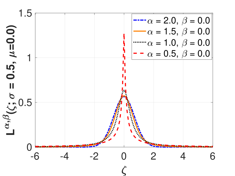
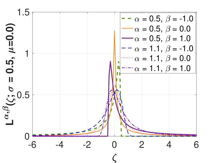
Figure 1: Probability density functions for Lévy distribution of $L^{\alpha,\beta}(\zeta;\sigma=0.5,\mu=0.0)$ with different values of the stability index and skewness parameters.

2.2 The excitable regime of the model

The deterministic memristive FHN neuron (i.e., Eq. (1) without the noise term) with a unique and stable fixed point cannot maintain a self-sustained spiking activity. One says in this case that the neuron is in the excitable regime [30], in contrast to the oscillatory regime, where the neuron continuously spikes due to the occurrence of a bifurcation onto a limit cycle. In the excitable regime, choosing an initial condition in the basin of attraction of this unique and stable fixed point will result in at most one large non-monotonic excursion into the phase space after which the trajectory returns to this fixed point and stays there until the initial conditions are changed again.

The deterministic predisposition required for SISR is an excitable regime, so that during SISR, the self-sustained and coherent spike trains produced by the neuron is due only to the presence of noise and not because of the occurrence of bifurcations onto a limit cycle. This is one of the crucial differences between SISR and CR — the predisposition required for the latter mechanism is the close proximity of parameters to the bifurcation threshold, so that weak noise amplitudes can easily drive the system to this bifurcation threshold without, stochastically, overwhelming the dynamics [64, 54, 10].

In this subsection, we determine the excitable regime of the memristive FHN neuron model in terms of the Hopf bifurcation and memristive parameters. At the fixed points $(v_{e},w_{e},\phi_{e})\in Fix$ (the set of rest states of the neuron), the variables $v(\tau)$, $w(\tau)$, and $\phi(\tau)$ reach a stationary state, while the set of fixed points defined by the intersection of the nullclines as

$$Fix:=\left\{(v,w,\phi)\in\mathbb{R}^{3}:f_{1}=f_{2}=f_{3}=0\right\},$$ (9)

depends on the parameters $c$, $d$, $k_{1}$, and $k_{2}$. The sign of

$$\Delta=\frac{g^{2}}{4}+\frac{p^{3}}{27},$$ (10)

determines the number of fixed points. In this paper, we consider the case where we have only one stable fixed point. If $\Delta>0$, we have a unique fixed point given by

$$\begin{split}\left\{\begin{array}[]{lcl}\displaystyle{v_{e}=\sqrt[3]{-\frac{g}{2}-\sqrt{\Delta}}+\sqrt[3]{-\frac{g}{2}+\sqrt{\Delta}}}\\[11.38109pt] \displaystyle{w_{e}=\frac{1}{c}(v_{e}+d)},\\[11.38109pt] \displaystyle{\phi_{e}=\frac{v_{e}}{k_{2}}},\end{array}\right.\end{split}$$ (11)

where

$$\begin{split}\left\{\begin{array}[]{lcl}p=\displaystyle{\frac{\frac{1}{c}+k_{1}a-1}{\frac{1}{3}+\frac{3k_{1}b}{k_{2}^{2}}}},\\[22.76219pt] g=\displaystyle{\frac{\frac{d}{c}}{\frac{1}{3}+\frac{3k_{1}b}{k_{2}^{2}}}}.\end{array}\right.\end{split}$$ (12)

Moreover, in the model we arbitrarily fix $d=0.5$ once and for all, and we determine the excitable regime of the model in terms of the parameter $c$ and the two new parameters $k_{1}$ and $k_{2}$ — also known as the magnetic gain parameters. With the fixed values of the parameters $a=0.1$, $b=0.02$, and $d=0.5$, $p$ and $g$ in Eq. (12) now depend only on $c$, $k_{1}$, and $k_{2}$. We have:

$$\begin{split}\left\{\begin{array}[]{lcl}p=\displaystyle{\frac{-1+\frac{1}{c}+0.1k_{1}}{\frac{1}{3}+\frac{0.06k_{1}}{k_{2}^{2}}}},\\[19.91692pt] g=\displaystyle{\frac{0.5}{c\Big{(}\frac{1}{3}+\frac{0.06k_{1}}{k_{2}^{2}}\Big{)}}},\end{array}\right.\end{split}$$ (13)

which are both always positive for $c<1,k_{1}\geq 0$ and $k_{2}>0$. Hence, $\Delta$ in Eq. (10) will always be positive for $c<1,k_{1}\geq 0$ and $k_{2}>0$, ensuring the uniqueness of the fixed point $(v_{e},w_{e},\phi_{e})$ in Eq. (11).

With initial conditions at the unique fixed point $\big{[}v_{e}(c,k_{1},k_{2}),w_{e}(c,k_{1},k_{2}),\phi_{e}(c,k_{1},k_{2})\big{]}$, we numerically computed a codimension-one and codimension-two bifurcations, showing the excitable and oscillatory regimes of the memristive neuron with the respect to the parameter $c$ in Fig. 2(a) and the magnetic gain parameters $k_{1}$ and $k_{2}$ in Fig. 2(b), respectively.

The bifurcation diagram in Fig. 2(a) shows a non-zero inter-spike interval ($ISI$) for $0<c<c_{h}$, where $c_{h}=0.875$ is the super-critical Hopf bifurcation threshold. For $c\geq c_{h}$, there is no spiking, i.e., $ISI=0$, indicating that the neuron is in an excitable regime at $k_{1}=0.1$ and $k_{2}=0.1$. However, it is well-known that variations in these magnetic gain parameters can significantly affect the dynamical response of the neuron [47], thereby switching the neuron’s dynamics from an excitable to an oscillatory regime and vice versa, even when $c>c_{h}$. Hence, it is important to determine the range of values of $k_{1}$ and $k_{2}$ in which the neuron will remain in the excitable regime for a particular value of $c$, chosen such that $c_{h}<c<1$.

Fig. 2(b) shows, for $c=0.95>c_{h}=0.875$ (i.e., $c$ is far enough from the bifurcation threshold and also less than one so that the stable fixed point is unique), a two-parameter space bifurcation diagram with respect to $k_{1}$ and $k_{2}$. We also note that $k_{2}$ starts at a non-zero value, i.e., at $k_{2}=0.01$, to ensure that our fixed point in Eq. (11) is unique. The color-coded $ISI$ shows the oscillatory regime in red and yellow where $ISI>0$. The yellow region corresponds to few points around the origin of the $(k_{1},k_{2})$ plane, where $ISI$ takes relatively large values. For example, at $k_{1}=0.0361$ and $k_{2}=0.01$ we have $ISI=10.16$, and at $k_{1}=0.0643$ and $k_{2}=0.03$, $ISI$ takes its largest value, i.e., $ISI=17.78$. The dark region (where $ISI=0$) corresponds to the excitable regime, with the deterministic model in Eq. (1) consisting of unique and stable fixed point given by Eq. (11). Therefore, throughout this paper, we will investigate the mechanism of SISR when the neuron is in the excitable regime defined by: $c=0.95$, $k_{1}\in[0.0,2.0]$, $k_{2}\in[1.0,2.0]$, $a=0.1$, $b=0.02$, $d=0.5$, and $\varepsilon=0.001\ll 1$.

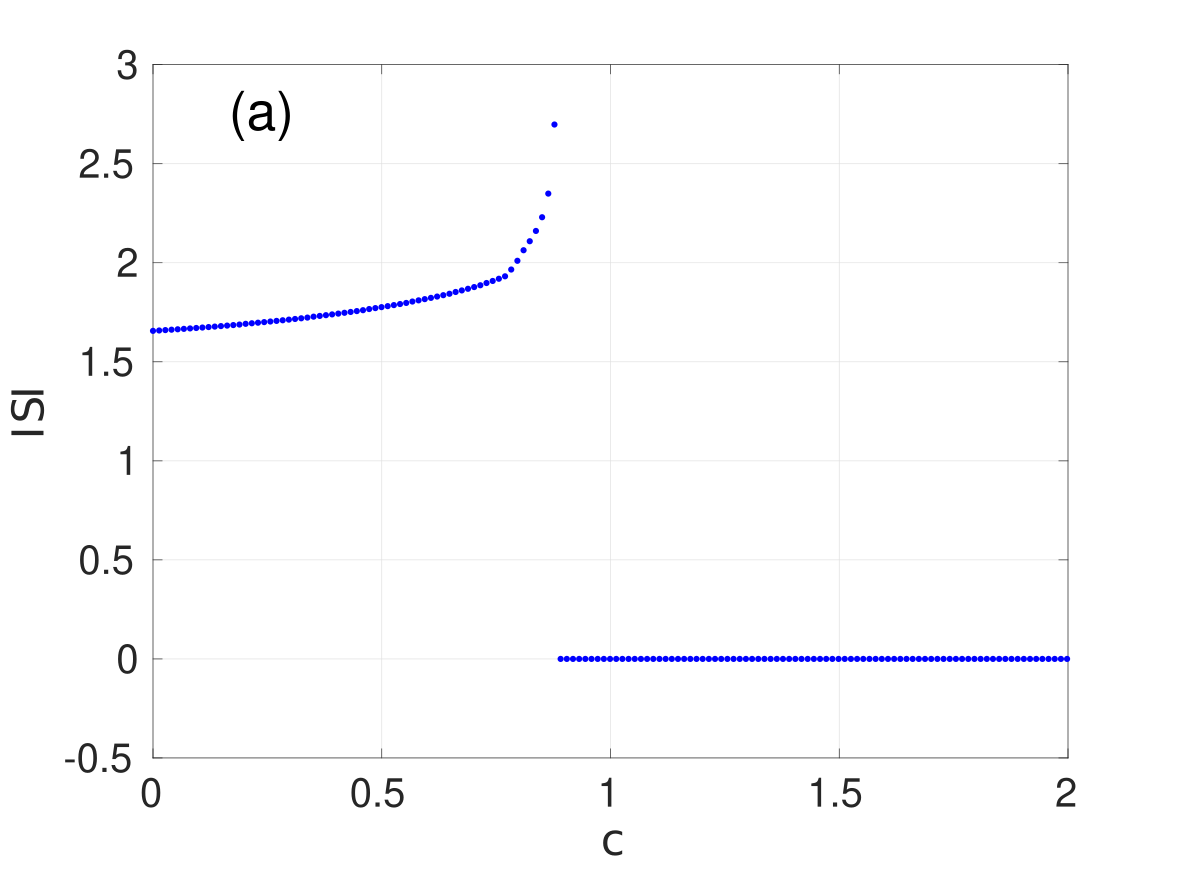
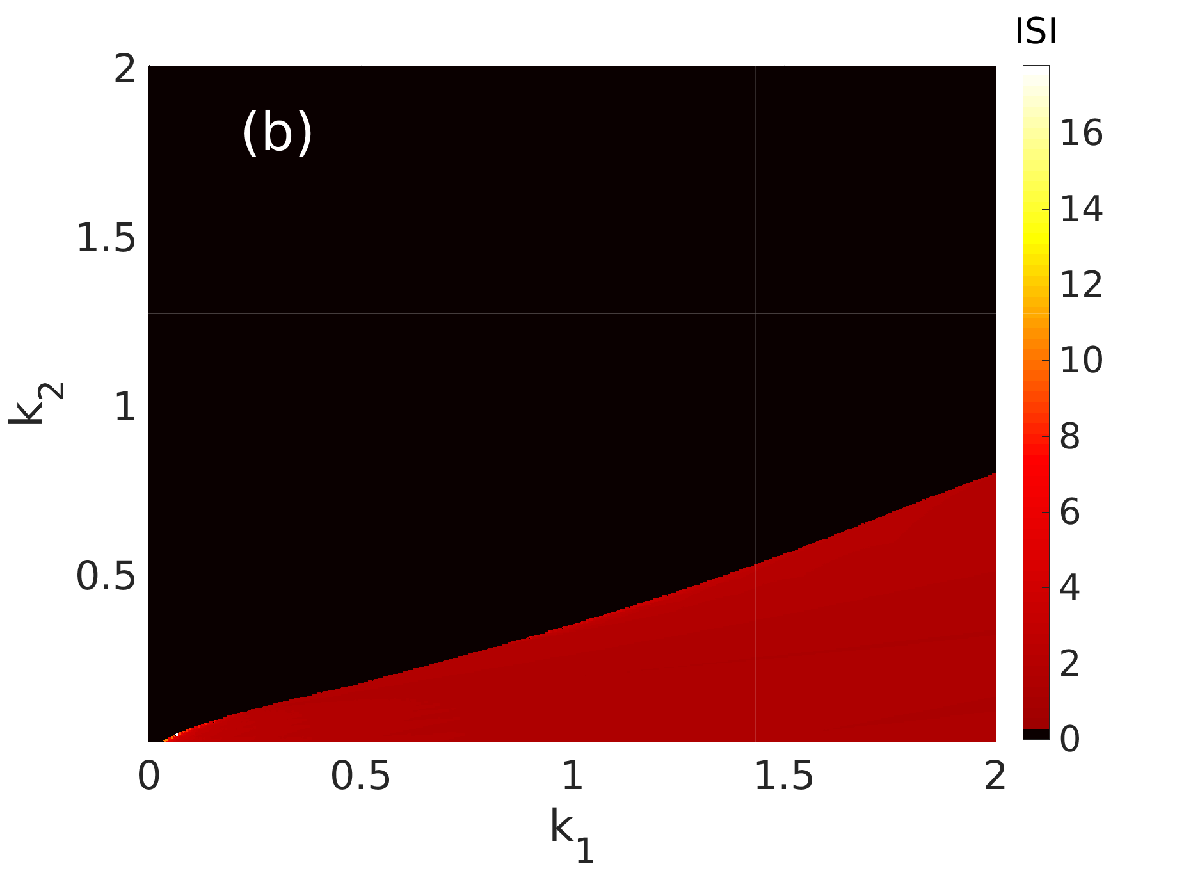
Figure 2: Panel (a): Bifurcation diagram with respect to parameter $c$, showing the oscillatory ($ISI>0$) and excitable ($ISI=0$) regimes in $c<c_{h}=0.875$ and $c\geq c_{h}$, respectively, with $k_{1}=0.1$ and $k_{2}=0.1$. Panel (b): Color-coded $ISI$ for a two-parameter space bifurcation diagram with respect to $k_{1}$ and $k_{2}$ at $c=0.95>c_{h}$, showing the oscillatory regime in red and yellow where $ISI>0$ and the excitable regime in dark where $ISI=0$. In both panels, the other parameter values are fixed at: $a=0.1$, $b=0.02$, $d=0.5$, and $\varepsilon=0.001$.

3 The asymptotic matching of timescales and SISR

Now we consider Eq. (1) such that its deterministic version is in the excitable regime, defined by the parameters intervals and values above. To understand how noise can induced a regular escape of trajectories from the basin of attraction of the stable fixed point, leading to the emergence of a coherent spike train, we transform Eq. (1) from the slow timescale $\tau$ to the fast timescale $t$ to obtain Eq. (14) using the relation $\varepsilon:=\tau/t$ or more precisely, $d\tau=\varepsilon dt$ [36]. Under this timescale transformation the noise term is re-scaled according to the scaling law of Lévy motion. That is, if $L_{\tau}$ is a Lévy motion, then for every $\lambda>0,\lambda^{-\frac{1}{\alpha}}L_{\lambda\tau}$ is also a Lévy motion (i.e., they have the same distribution). Furthermore, we consider the standard form of the Lévy noise, i.e., $L^{\alpha,\beta}(\tau;\sigma,0)=\sigma\hat{L}^{\alpha,\beta}(\tau;1,0)$, where the scale parameter $\sigma$ clearly represents the noise intensity. We note that because of this scaling law, the term $1/\sqrt[\alpha]{\varepsilon}$ was introduced in the noise term in Eq. (1) to guarantee that in Eq. (14), the noise intensity, $\sigma$, measures the relative strength of the noise term compared to the deterministic term $f_{1}(v_{t},w_{t},\phi_{t})$ irrespective of the value of $\varepsilon$.

$$\begin{split}\left\{\begin{array}[]{lcl}dv_{t}&=&f_{1}(v_{t},w_{t},\phi_{t})dt+\sigma d\hat{L}_{t}^{\alpha,\beta},\\[8.53581pt] dw_{t}&=&\varepsilon f_{2}(v_{t},w_{t},\phi_{t})dt,\\[8.53581pt] d\phi_{t}&=&\varepsilon f_{3}(v_{t},w_{t},\phi_{t})dt.\end{array}\right.\end{split}$$ (14)

In the adiabatic limit $\varepsilon\to 0$, the timescale separation between $v_{t}$ and the two other variables $w_{t}$ and $\phi_{t}$ become very large. This indicates that $w_{t}$ and $\phi_{t}$ are frozen on the $O(1)$ fast timescale. Hence, Eq. (14) is approximated by Eq. (15)

$$\begin{split}\left\{\begin{array}[]{lcl}dv_{t}&=&-U_{k_{1}}^{\prime}(v_{t})dt+\sigma d\hat{L}^{\alpha,\beta}_{t},\\ dw_{t}&=&0,\\ d\phi_{t}&=&0,\\ \end{array}\right.\end{split}$$ (15)

where $U_{k_{1}}^{\prime}(v_{t})$ is the derivative of the potential

$$U_{k_{1}}(v)=\frac{1}{12}v^{4}-\frac{1-k_{1}\rho(\phi)}{2}v^{2}+wv,$$ (16)

with respect $v$. $U_{k_{1}}(v)$ is the double-well potential with the constant solutions of the last two equations in Eq. (15) given by $w$ and $\phi$, respectively. This potential has, respectively, a left local minimum, a saddle, and a right local minimum at

$$\begin{split}\left\{\begin{array}[]{lcl}v_{l}&=&2\sqrt{-\frac{P}{3}}\cos\Bigg{(}\frac{1}{3}\arccos\Bigg{(}\frac{3Q}{2P}\sqrt{\frac{-3}{P}}\Bigg{)}+\frac{2\pi}{3}\Bigg{)},\\[11.38109pt] v_{m}&=&2\sqrt{-\frac{P}{3}}\cos\Bigg{(}\frac{1}{3}\arccos\Bigg{(}\frac{3Q}{2P}\sqrt{\frac{-3}{P}}\Bigg{)}-\frac{2\pi}{3}\Bigg{)},\\[11.38109pt] v_{r}&=&2\sqrt{-\frac{P}{3}}\cos\Bigg{(}\frac{1}{3}\arccos\Bigg{(}\frac{3Q}{2P}\sqrt{\frac{-3}{P}}\Bigg{)}\Bigg{)},\end{array}\right.\end{split}$$ (17)

where $P=3[k_{1}\rho(\phi)-1]$ and $Q=3w$, see Fig. 3.

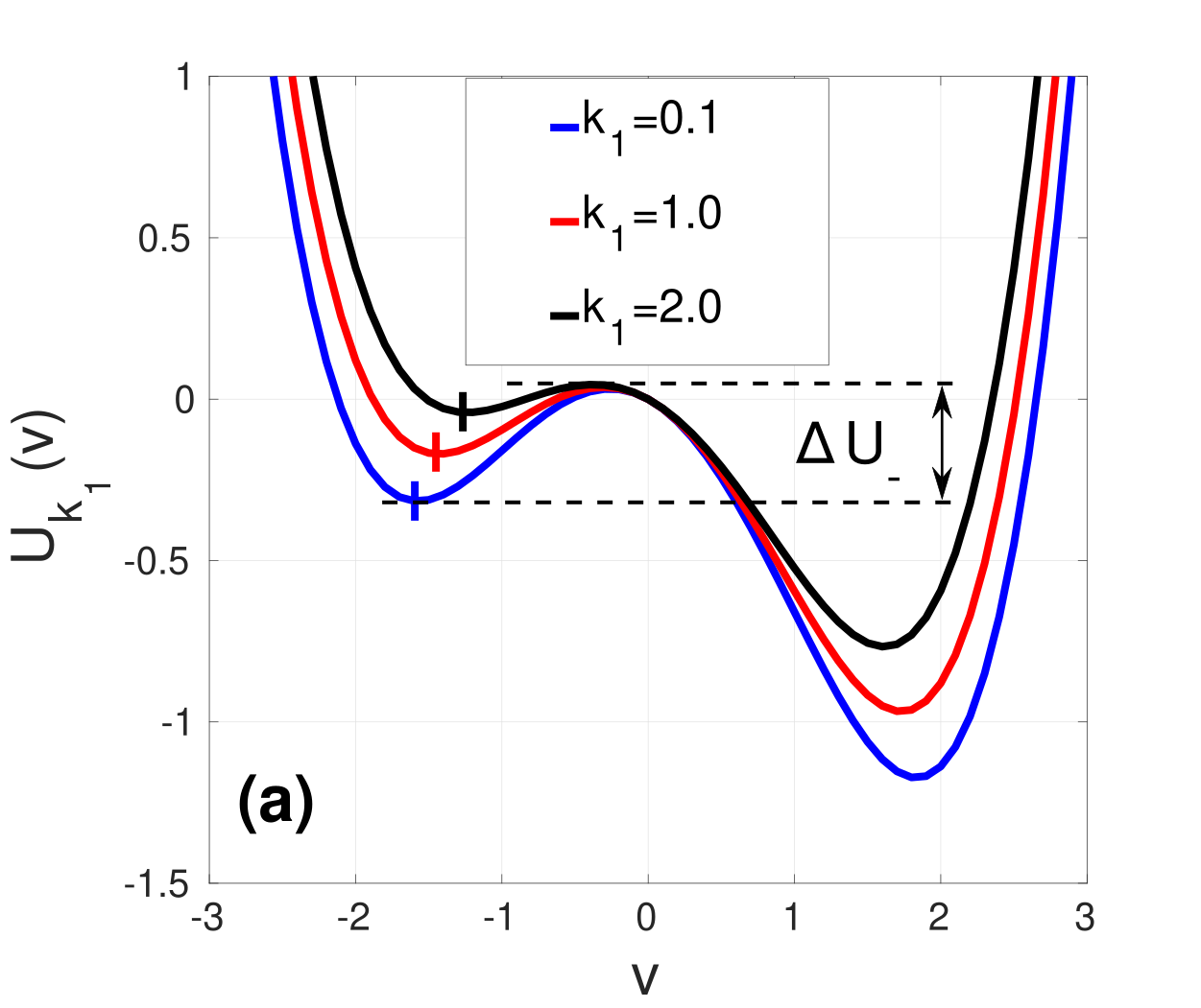
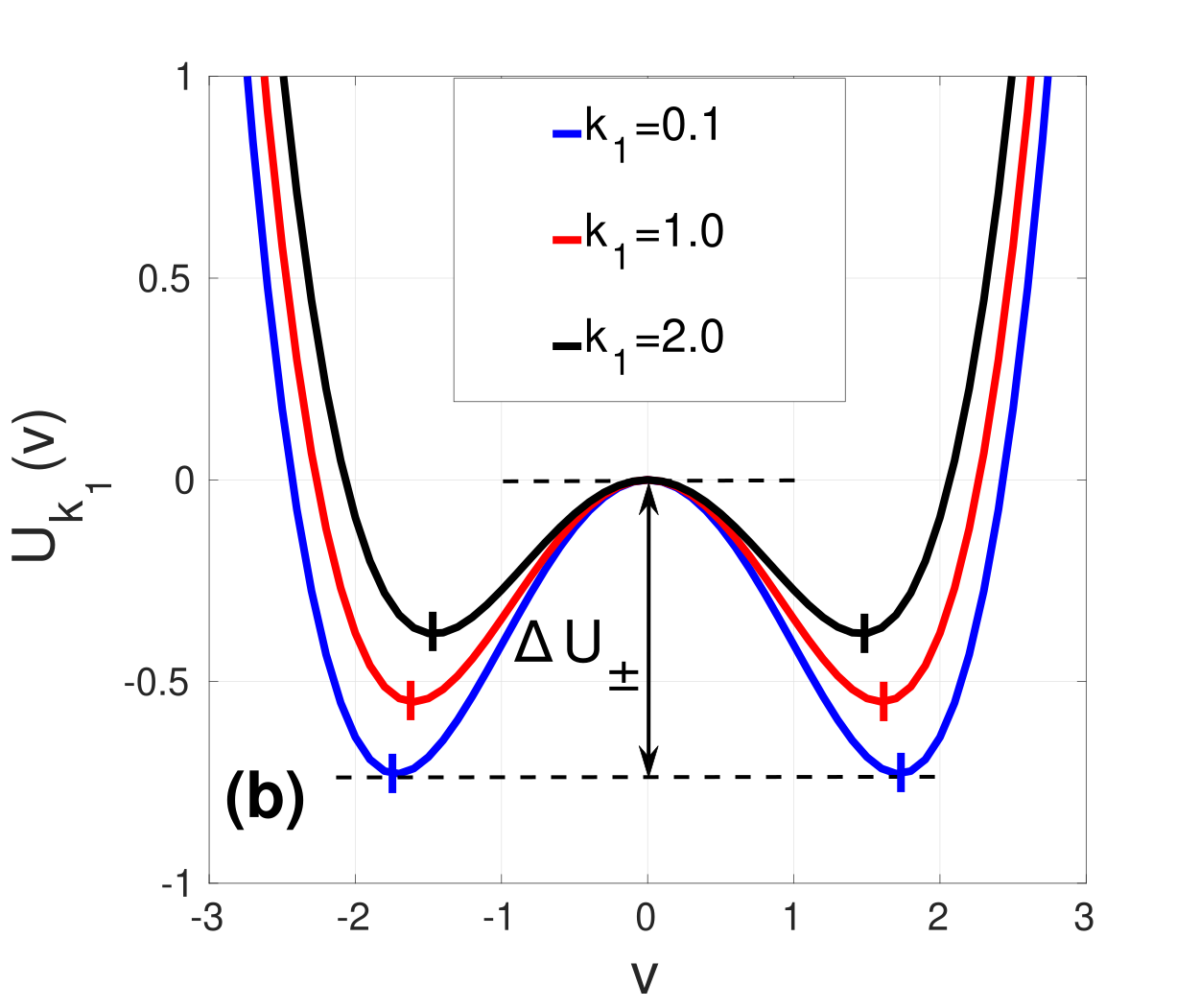
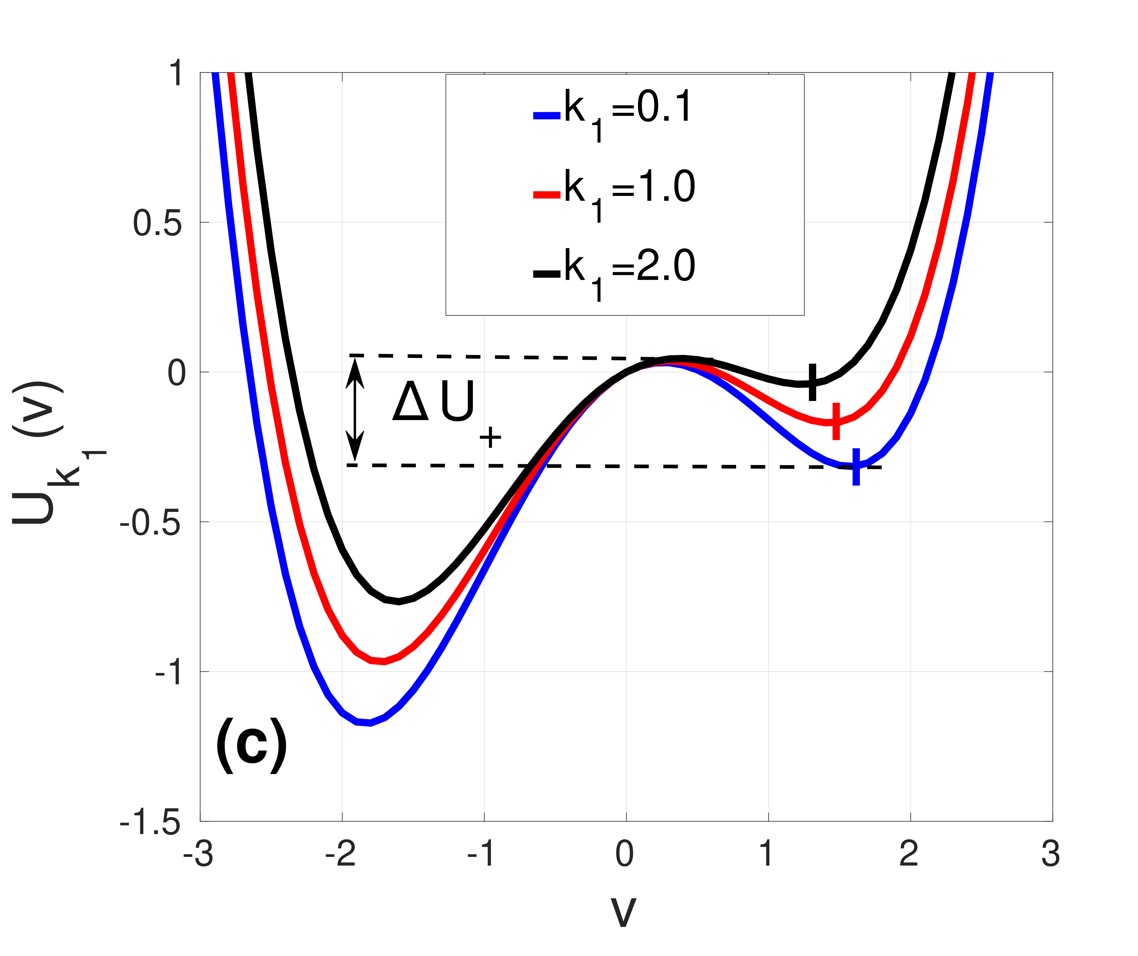
Figure 3: Variations of the potential $U_{k_{1}}(v)$ given in Eq. (16). The energy barriers $\bigtriangleup U_{\pm}$ are indicated in the asymmetric cases in (a) ($w<0$) and in (c) ($w>0$), and in the symmetric case in (b) ($w=0$). The band widths of the wells are given by the distances between the minima located at $v_{l}$ and $v_{r}$ (short vertical bars) and the saddle point located at $v=v_{m}=0$. The stronger the magnetic gain parameter $k_{1}$, the shallower the energy barriers $\bigtriangleup U_{\pm}$ and the shorter the band widths. In (a), $w=-0.25$, in (c) $w=0.25$, and in all panels $\phi=0.85$.

It was shown in [6, 29] that for barrier crossing phenomena driven by Lévy white noise in the double-well potential, the mean exit time from one of the wells increases as a power $\sigma^{-\alpha}$ of the noise intensity $\sigma$ with $\sigma\to 0$ and not exponentially as with Gaussian white noise would do in the limit as $\sigma\to 0$ [90, 34, 73]. By applying the general results presented in [29] to our particular case, we calculated for the double-well potential in Eq. (16), the mean exit times of the Lévy process as:

$$\begin{split}\left\{\begin{array}[]{lcl}\displaystyle{\mathbb{E}T_{exit}(v_{l}\to v_{r})\approx\frac{\alpha|v_{l}|^{\alpha}}{\sigma^{\alpha}}},\>\text{as}\>\sigma\to 0\\[8.53581pt] \displaystyle{\mathbb{E}T_{exit}(v_{r}\to v_{l})\approx\frac{\alpha v_{r}^{\alpha}}{\sigma^{\alpha}}},\>\text{as}\>\sigma\to 0.\end{array}\right.\end{split}$$ (18)

We note that the mean exit times in Eq. (18) depend on the location of the local minima $v_{l}$ and $v_{r}$. We further recall that the mean exit times of the processes driven by $\alpha$-stable noise are much shorter than those of Gaussian processes because of the presence of large jumps which occur with probability polynomially small in $\sigma$ [29].

On the other hand, the mean exit times of the Gaussian process follow Kramers’ law [90, 34], with escape events occurring with exponentially small probabilities, and are given by:

$$\begin{split}\left\{\begin{array}[]{lcl}\displaystyle{\mathbb{E}T_{exit}(v_{l}\to v_{r})\approx\exp\bigg{(}\frac{2\bigtriangleup U_{-}}{\sigma^{2}}\bigg{)}},\>\text{as}\>\sigma\to 0\\[11.38109pt] \displaystyle{\mathbb{E}T_{exit}(v_{r}\to v_{l})\approx\exp\bigg{(}\frac{2\bigtriangleup U_{+}}{\sigma^{2}}\bigg{)},\>\text{as}\>\sigma\to 0},\end{array}\right.\end{split}$$ (19)

where $\bigtriangleup U_{\pm}$ are the energy barrier functions that depend, technically, on $w$ and $\phi$. The asymmetry of the potential in Eq. (16) is controlled only by the sign of the coefficient of the linear term, i.e., the sign of $w$. While the depths of the wells $\bigtriangleup U_{\pm}$ are controlled by the value of $w$ and more significantly, by the term $k_{1}\rho(\phi)/2$. But in the limit as $\varepsilon\to 0$ in Eq. (14), the magnetic variable $\phi$ becomes almost constant and only the magnetic gain parameter $k_{1}$ now significantly changes the depths of the potential wells $\bigtriangleup U_{\pm}$. So we can drop the $\phi$ dependence in the energy barrier functions and write them as:

$$\begin{split}\left\{\begin{array}[]{lcl}\bigtriangleup U_{-}(w):=U_{k_{1}}(v_{m})-U_{k_{1}}(v_{l}),\\[2.84526pt] \bigtriangleup U_{+}(w):=U_{k_{1}}(v_{m})-U_{k_{1}}(v_{r}).\end{array}\right.\end{split}$$ (20)

Thus, in the Gaussian case, the trajectories surmount the potential barriers $\bigtriangleup U_{\pm}$, such that the mean exit times depend exponentially on the depth of the potential well.

We notice in Fig. 3 that the depths of these barriers are inversely proportional to the strength of the magnetic gain parameter $k_{1}$. Thus, a stronger magnetic flux due to a larger value of $k_{1}$ should, on average, reduce the duration of the mean exit times of the trajectory perturbed by Gaussian noise, contributing to an increase in the spiking frequency.

On the other hand, we also notice that the positions of the minima (at $v_{l}$ and $v_{r}$, indicated by the short vertical bars in Fig. 3) with respect to the fixed saddle (at $v_{m}=0.0$) change with $k_{1}$. We observe that the stronger magnetic flux $k_{1}$, the smaller the distances of $v_{l}$ or $v_{r}$ from $0.0$, which in turn shortens, on average, the duration of the mean exit times of the trajectory perturbed by Lévy noise, contributing to an increase in the spiking frequency.

From Eq. (1), the deterministic timescale at which trajectories move on the stable parts of the 2-dimensional cubic nullcline of the current model, given by $w(v,\phi)=-\frac{v^{3}}{3}+(1-k_{1}\rho(\phi))v$ (not shown), is $\varepsilon^{-1}$ [90]. When there is no noise ($\sigma=0$), the neuron is in the excitable regime and as $\varepsilon\to 0$, trajectories tend to spend a lot of time moving adiabatically along the stable parts of the 2D cubic nullcline, toward the unique stable fixed point at $(v_{e},w_{e},\phi_{e})$ given by Eq. (11), where it stops and stays for ever until a new perturbation is provoked by, e.g., a random process.

When noise is switched on ($\sigma\neq 0$), it may kick a trajectory, which is moving quasi-deterministically at a timescale of $\varepsilon^{-1}$ along one stable branch of the 2D cubic nullcline, to another branch and then back. This corresponds to jumps out of the left and right potential wells, thereby causing a spike — an oscillation. Depending on the type of noise perturbing the neuron, an escape from left to right (right to left) occurs at the stochastic timescale $\mathbb{E}T_{exit}$ given by the first (second) equation of Eq. (18) for the Lévy process or Eq. (19) for the Gaussian process.

It has been shown that the occurrence of SISR crucially depends on the neuron’s ability to asymptotically match, with probability close to unity, the deterministic timescale $\varepsilon^{-1}$ (i.e., timescale at which a trajectory moves along the stable parts of the 2D cubic nullcline) and the stochastic timescale $\mathbb{E}T_{exit}$ (i.e., the timescale at which this trajectory escapes from the stable parts of this nullcline) at unique exit points $w_{-}$ and $w_{+}$ located, respectively, on the left and right stable branches of the 2D cubic nullcline [89, 52, 10, 51, 9, 11, 71, 90, 92, 88].

If the deterministic timescale is shorter than the stochastic timescales (i.e., $\varepsilon^{-1}<\mathbb{E}T_{exit}$), then the trajectory has no time to escape from the left and right stable branches of the cubic nullcline which respectively correspond to the left and right wells of the potential $U_{k_{1}}(v)$. Because the neuron is in an excitable regime, the trajectory gets trapped in the left well of the potential (i.e., on the left stable branch of the cubic nullcline on which the unique stable fixed point is located) for too long. In this scenario, a spike is a rare event and this could destroy the coherence of the spiking, especially for short time intervals.

On the other hand, if the deterministic timescale is longer than the stochastic timescales (i.e., $\varepsilon^{-1}>\mathbb{E}T_{exit}$), then the trajectory frequently escape from the potential wells (i.e., the stable branches of the cubic nullcline). In this scenario, spiking is frequent (i.e., not rare) but incoherent because the trajectory escapes at several different points on the each of the stable branches of the cubic nullcline.

Interestingly, if at specific and unique points $w_{-}$ and $w_{+}$ on respectively the left and right stable branch of the cubic nullcline, the deterministic timescale matches the stochastic timescales (i.e., $\varepsilon^{-1}=\mathbb{E}T_{exit}$), frequent and coherent spiking emerges — SISR occurs. The uniqueness of the exit points $w_{-}$ and $w_{+}$ can only be guaranteed by the monotonicity of the minima $v_{l}(w)$ and $v_{r}(w)$ in the case of Lévy noise (see Eq. (21)) and the barrier functions $\bigtriangleup U_{-}(w)$ and $\bigtriangleup U_{+}(w)$ in the case of Gaussian noise (see Eq. (22)).

In Fig. 4, we show the graphs of the functions $|v_{l}|$, $v_{r}$, $\bigtriangleup U_{-}$, and $\bigtriangleup U_{+}$ with respect to $w\in[-\frac{2}{3},\frac{2}{3}]$, where the lower and upper bounds of this interval correspond to the $w$-coordinate of the local minimum and maximum of the cubic nullcline, respectively. Here, we see that these functions are all monotone with respect to $w\in[-\frac{2}{3},\frac{2}{3}]$. Hence, frequent and coherent spiking would occur if we match the deterministic and stochastic timescales only at $w_{-}$ on the left stable branch and at $w_{+}$ on the right stable branch of the cubic nullcline, that is:

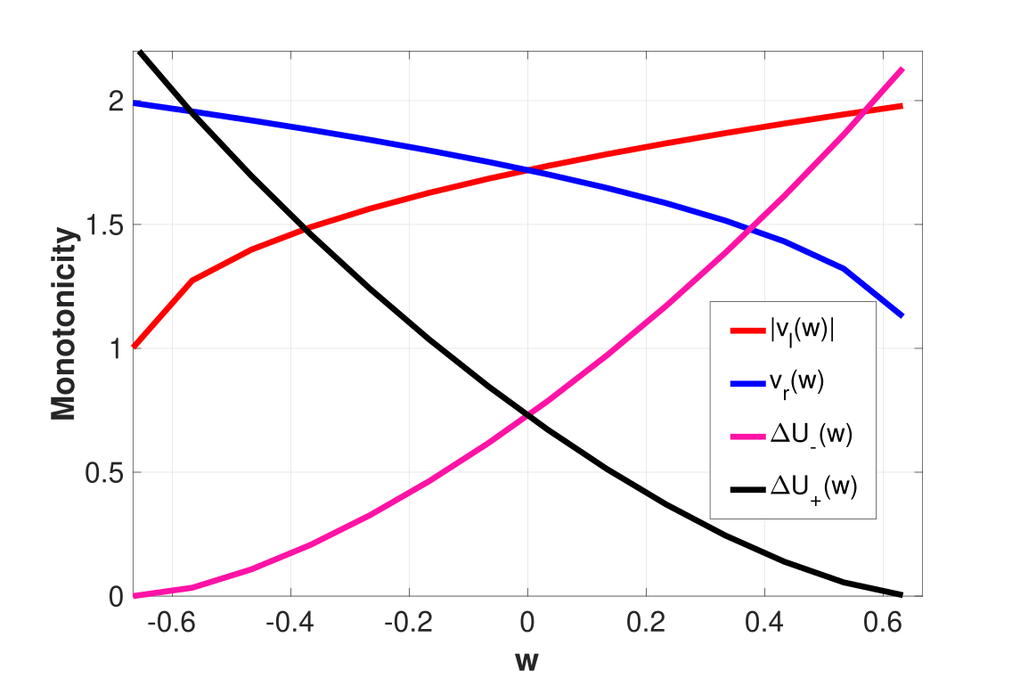
Figure 4: The graphs of the $|v_{l}(w)|$, $v_{r}(w)$, $\bigtriangleup U_{-}(w)$, and $\bigtriangleup U_{+}(w)$ with respect to $w\in[-\frac{2}{3},\frac{2}{3}]$. Their monotonicity ensure the uniqueness of the escape points $w_{-}$ and $w_{+}$ which satisfy the equations in Eq. (21) and Eq. (22). Parameters are $k_{1}=0.1$ and $\phi=0.85$.

$$\begin{split}\displaystyle{\frac{\alpha|v_{l}(w_{-})|^{\alpha}}{\sigma^{\alpha}}}=\frac{1}{\varepsilon}=\displaystyle{\frac{\alpha v_{r}(w_{+})^{\alpha}}{\sigma^{\alpha}}},\end{split}$$ (21)

for the Lévy process, and

$$\begin{split}\displaystyle{\exp\bigg{(}\frac{2\bigtriangleup U_{-}(w_{-})}{\sigma^{2}}\bigg{)}}=\frac{1}{\varepsilon}=\displaystyle{\exp\bigg{(}\frac{2\bigtriangleup U_{+}(w_{+})}{\sigma^{2}}\bigg{)}},\end{split}$$ (22)

for the Gaussian process. Therefore, the occurrence of SISR (i.e., frequent and coherent spiking activity) will depend on the neurons’ ability to asymptotically match the timescales by taking the following double scaling limits:

$$\begin{split}\displaystyle{\lim\limits_{(\varepsilon,\sigma)\rightarrow(0,0)}}\bigg{[}\sigma^{\alpha}\varepsilon^{-1}\bigg{]}\to\left\{\begin{array}[]{lcl}\displaystyle{\alpha|v_{l}(w_{-})|^{\alpha}}\\[5.69054pt] \displaystyle{\alpha v_{r}(w_{+})^{\alpha}}\end{array}\right.\end{split}$$ (23)

for the Lévy process, and

$$\begin{split}\displaystyle{\lim\limits_{(\varepsilon,\sigma)\rightarrow(0,0)}}\Bigg{[}\frac{\sigma^{2}\ln(\varepsilon^{-1})}{2}\Bigg{]}\to\left\{\begin{array}[]{lcl}\displaystyle{\bigtriangleup U_{-}(w_{-})}\\[5.69054pt] \displaystyle{\bigtriangleup U_{+}(w_{+})}\end{array}\right.\end{split}$$ (24)

for the Gaussian process [52, 90].

Due to the anomalous long jumps of a trajectory perturbed by a Lévy process [29, 32, 16, 12], this trajectory does not necessarily have to hit the saddle point at $v_{m}$ before escaping from the stable branches of the 2D cubic nullcline. Hence, escapes may instantaneously occur even with a very weak noise intensity. This means that the “frequent spiking” requirement of SISR can be easily achieved by a Lévy process, even with a very weak intensity. However, the “coherent spiking” requirement of SISR can only be guaranteed by the asymptotic scaling limits given in Eq. (23).

In the Gaussian case, a trajectory can only escape from a potential well after hitting the boundary at the saddle point at $v_{m}$. Therefore, the “frequent spiking” requirement of SISR needs that the noise intensity is not too weak (otherwise, we get a Poissonian spike train — a rare spiking event which could destroy the coherence of the spiking [90]). Moreover, we observe that the stochastic timescales of the Gaussian noise in Eq. (19) depend on the energy barrier functions $\bigtriangleup U_{\pm}$. If these barriers are too deep (i.e., $\bigtriangleup U_{\pm}\to\infty$), then weak noise intensities cannot provoke escapes (at least frequently), and the trajectory will remain strapped inside a potential well. Thus, the noise has be to weak (so that the mean exit times satisfy Eq. (19)), but strong enough to able to invoke some spiking. If this Gaussian noise is strong enough to invoke spiking, then the “coherent spiking” requirement of SISR can only be guaranteed by the asymptotic scaling limits given by Eq. (24). Thus, for Lévy noise, we expect SISR to occur even at very weak noise intensities. But for Gaussian noise, we expect SISR to occur at a comparatively larger intensity.

To answer the three main questions we are interested in (see the introduction section), we will set the memristive neuron in the excitable regime by choosing $c=0.95$, $a=0.1$, $b=0.02$, $d=0.5$, and also set location parameter of the standardized Lévy process at $\mu=0.0$. We chose a sufficiently small timescale separation parameter, i.e., $\varepsilon=0.001\ll 1$, weak noise intensity, i.e., $0<\sigma<1$, and then numerically search for the combined values of $k_{1}\in[0.0,2.0]$, $k_{2}\in[1.0,2.0]$, $\alpha\in(0,2]$, and $\beta\in[-1,1]$ for which the scaling limit conditions in Eq. (23) and Eq. (24) are satisfied (or at least to some degree) or not.

4 Numerical results and discussion

To measure the degree of SISR (i.e., the degree to which Eq. (23) and Eq. (24) are satisfied), we use the coefficient of variation ($CV$), an important statistical measure based on the time intervals between spikes [64]. From a neurobiological point of view, $CV$ is more important than other measures (e.g., power spectral density and auto-correlation function) because it is related to the timing precision of information processing in neural systems [59]. $CV$ uses the inter-spike intervals (ISIs) where the $k$th interval is the difference between two consecutive spike times $t^{k}$ and $t^{k+1}$ of the neuron, and is defined as:

$$CV=\dfrac{\sqrt{\langle ISI^{2}\rangle-\langle ISI\rangle^{2}}}{\langle ISI\rangle},$$ (25)

where $\langle ISI\rangle$ and $\langle ISI^{2}\rangle$ represent the mean and the mean squared ISIs, respectively. When $CV=1$, we have Poissonian spike train (i.e., rare and incoherent spiking), and when $CV>1$ we have a point process that is even more variable than a Poisson process [37]. In both these cases, the degree of SISR is quite low as the double limits in the left-hand sides of Eq. (23) and Eq. (24) fail to converge toward the corresponding values on the right-hand sides. The degree of SISR becomes higher with $CV\to 0$ as the double limits in the left-hand sides of Eq. (23) and Eq. (24) also converge toward the corresponding values on the right-hand sides. When $CV=0$, the double limits in the left-hand sides of Eq. (23) and Eq. (24) should be exactly equal to the corresponding values on the right-hand sides. In this case, we will have perfectly “deterministic” periodic spiking.

For our numerical simulations, we used the fourth-order stochastic Runge-Kutta algorithm employed in [28, 86, 76] and proven in [67] to strongly converge. In should be noted that for general noise, the numerical solution of stochastic differential equations that uses the scheme proposed by Wilkie [79] may not be intact even with additive noise, see also [4].

We generate the Lévy random variable by using the Janicki-Weron algorithm [31] which has been proven [95, 77] to generate stable random variable for all admissible values of the parameters $\alpha$, $\beta$ $\mu$, and $\sigma$. We numerically integrate Eq. (14) for a very long time interval (i.e., $T=4\times 10^{7}$ time unit which allows for the small value of $\varepsilon=0.001$, the collection of sufficiently many ISIs for statistical estimate). We then average the ISIs over time and up to $30$ realizations for each noise amplitude.

We recall that the continuous jump property of a Gaussian process (with finite variance) forces the trajectories to hit the boundary of a domain before escaping. While with the discontinuous long-jumps of a Lévy process with $\alpha<2$ (with infinite variance), trajectories can rapidly escape to infinity without hitting the boundary. Thus, for our FHN neuron perturbed by a Lévy noise, we might need to wait for a long time for a trajectory which had exhibited a long-jump to come back to the vicinity of the stable fixed point, if there is no compulsory truncation. It is important to note that these long waiting times can significantly affect the ISIs. Hence, because the $CV$ (used to characterised the degree of SISR) depends (only) on the ISIs, the numerical results obtained would be sensitive to the choice of the truncation threshold. Considering the physical and computer saturation effects, a suitable truncation scheme should, therefore, be adoptable. In our simulations, we use the truncation threshold $v=3.0$ $\times$ sign$(v)$ whenever $\lvert v\rvert>3.0$. This is a well-known truncation scheme for $\alpha$-stable noises employed in many relevant references [33, 50, 42].

To avoid the long waiting times to which CV is sensitive to, we decided to use the truncation threshold above. We note that the threshold values (i.e., $v=-3$ and $v=3$) are respectively below and above, but also sufficiently close to the extreme values ($v=-2$ and $v=2$, see Fig. 5(d)) of the relaxation oscillations of the underlining deterministic FHN model. A value of, for example, $v=1000$ is not physiological for the FHN model. Thus, the truncation threshold used not only ensures that the simulated trajectories do not escape to infinity (thereby avoiding the long waiting times) but also ensures that the trajectories go not too far below and above the extreme values of the relaxation oscillation, which are in fact the physiologically acceptable extreme values for the model. In the presence of noise, the random trajectories may then oscillate with slightly bigger amplitudes compared to that of the deterministic relaxation oscillation. Thus, the truncation scheme used gives room for these fluctuations to be taken into account without any significant effect on the waiting times that arise due to the long-jumps. These makes the truncation threshold $v=3\times sign(v)$ whenever $|v|>3$, a good ans natural choice when calculating the CV values of the FHN model perturbed by a Lévy noise.

Fig. 5(a) and (c) respectively show the variation of $CV$ with the noise intensity $\sigma$ for a very impulsive ($\alpha=0.1$) and symmetric ($\beta=0.0$) Lévy noise and a time series of the coherent spike trains obtained at a noise intensity that satisfies Eq. (23). The $CV$-curve and time series are computed in a weak magnetic flux regime ($k_{1}=0.1$, $k_{2}=0.1$) and show that as long as Eq. (23) is valid, Lévy noise can $(i)$ induce a high degree of SISR even at very weak noise intensities (e.g., $CV\approx 0.075$ at $\sigma=1.0\times 10^{-15}$), and $(ii)$ induce an even higher degree of SISR at relatively larger noise intensities (e.g., $CV=0.0015$ at $\sigma\approx 0.9$). It is worth noting that in Fig. 5(a) and (c) the Lévy noise is very impulsive, i.e., the stability index is very small ($\alpha=0.1$), and therefore even at very weak noise intensities (such as $\sigma=1.0\times 10^{-20}$), the long-jumps can still occasionally occur, thereby inducing some spikes whose $ISIs\neq 0$ will contribute to a finite CV value. But as $\alpha$ increases, the long-jumps become less frequent and of shorter range. Thus, only relatively larger noise intensities can invoke spikes as in Gaussian case in Fig. 5(b) and (d).

In Fig. 5(b) and (d), we respectively show the variation of $CV$ with the noise intensity $\sigma$ for Gaussian noise ($\alpha=2.0$, $\beta=0.0$) and a time series of the coherent spike train obtained at a noise intensity which satisfies Eq. (24), in the same weak magnetic flux regime ($k_{1}=0.1$, $k_{2}=0.1$). Comparing the degree of SISR induced by a Lévy noise with parameters at $\alpha=0.1$ and $\beta=0.0$ to that of Gaussian noise ($\alpha=2.0$, $\beta=0.0$), we see that Lévy noise can induce a higher degree of SISR with both extremely weak and weak noise amplitudes. In Fig. 5(b) with Gaussian noise, we have a low (and almost constant) $CV\approx 0.045$ only in the weak (but not too weak) noise intensities, i.e., for $\sigma\in(0.01,0.1)$.

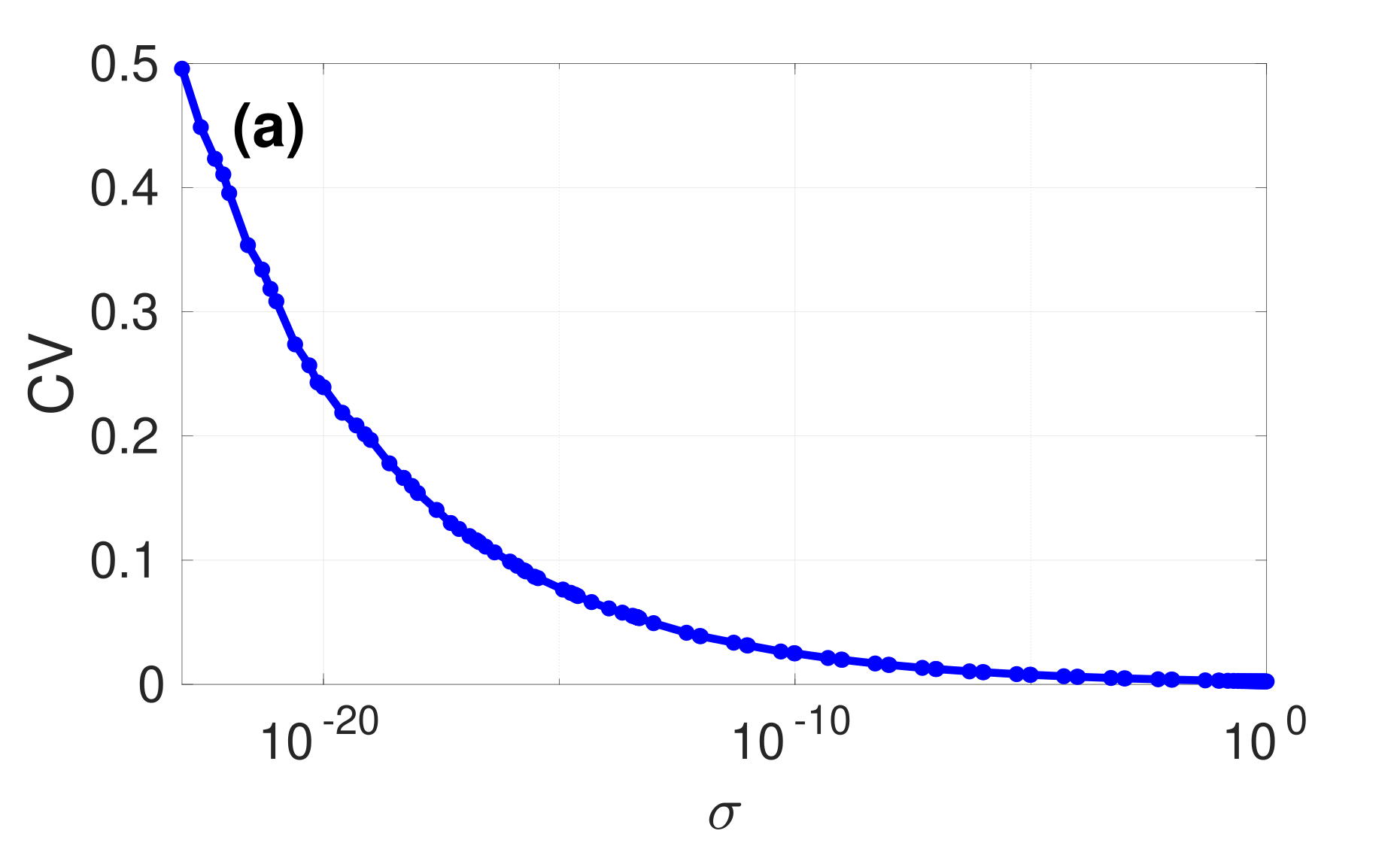
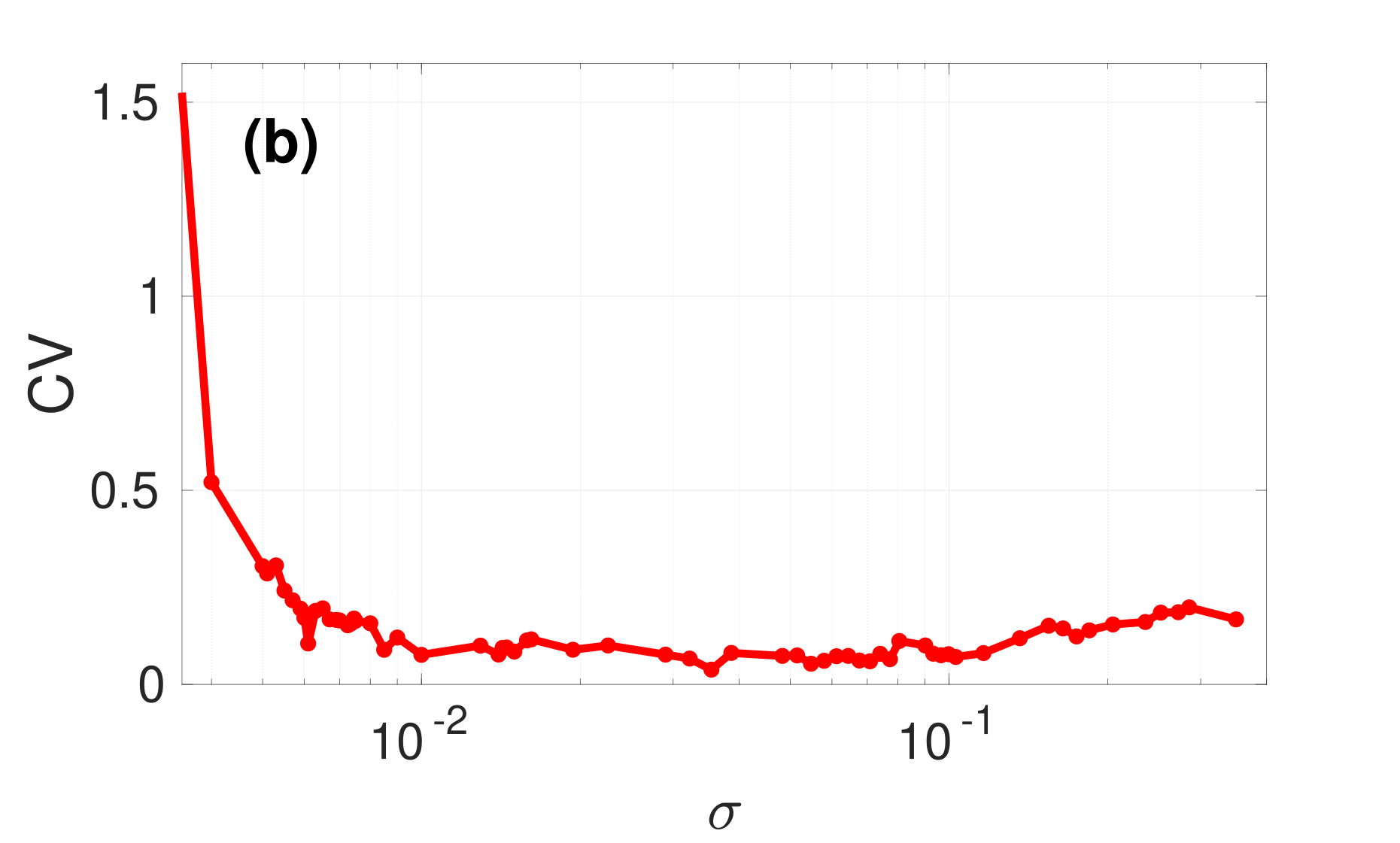
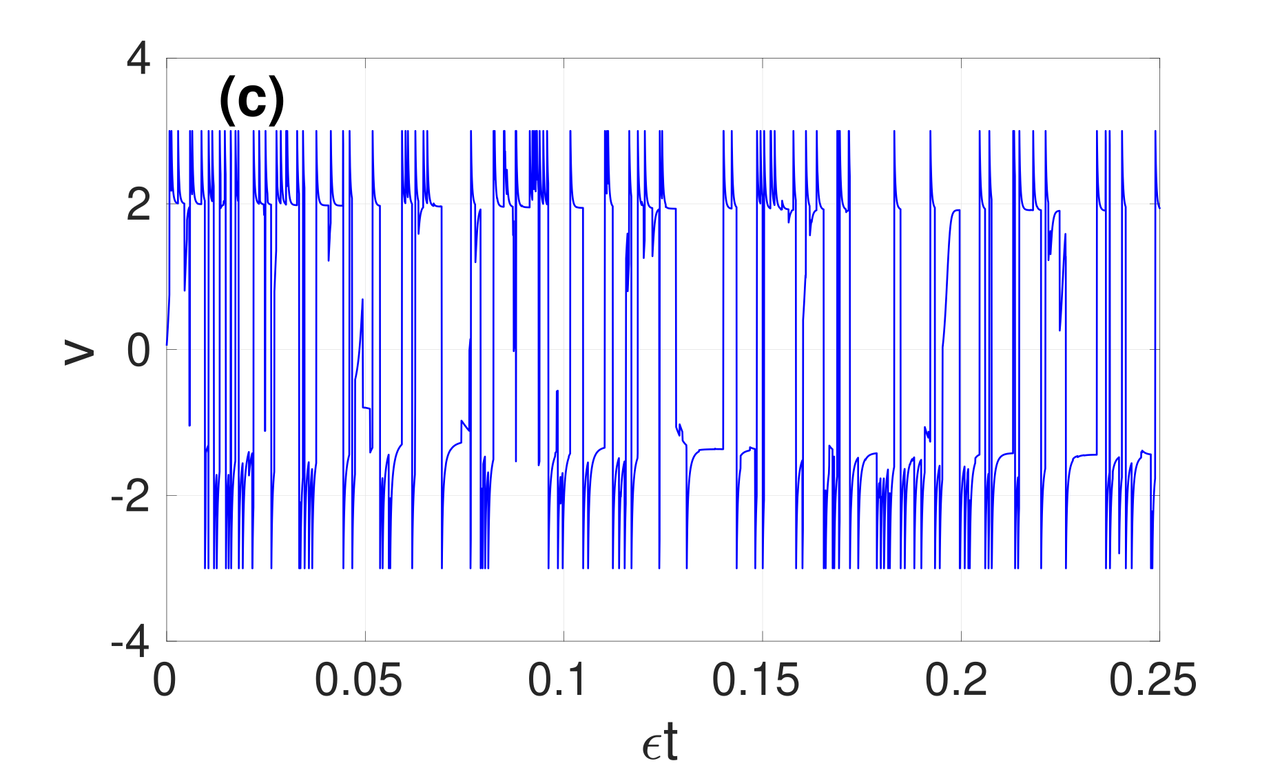
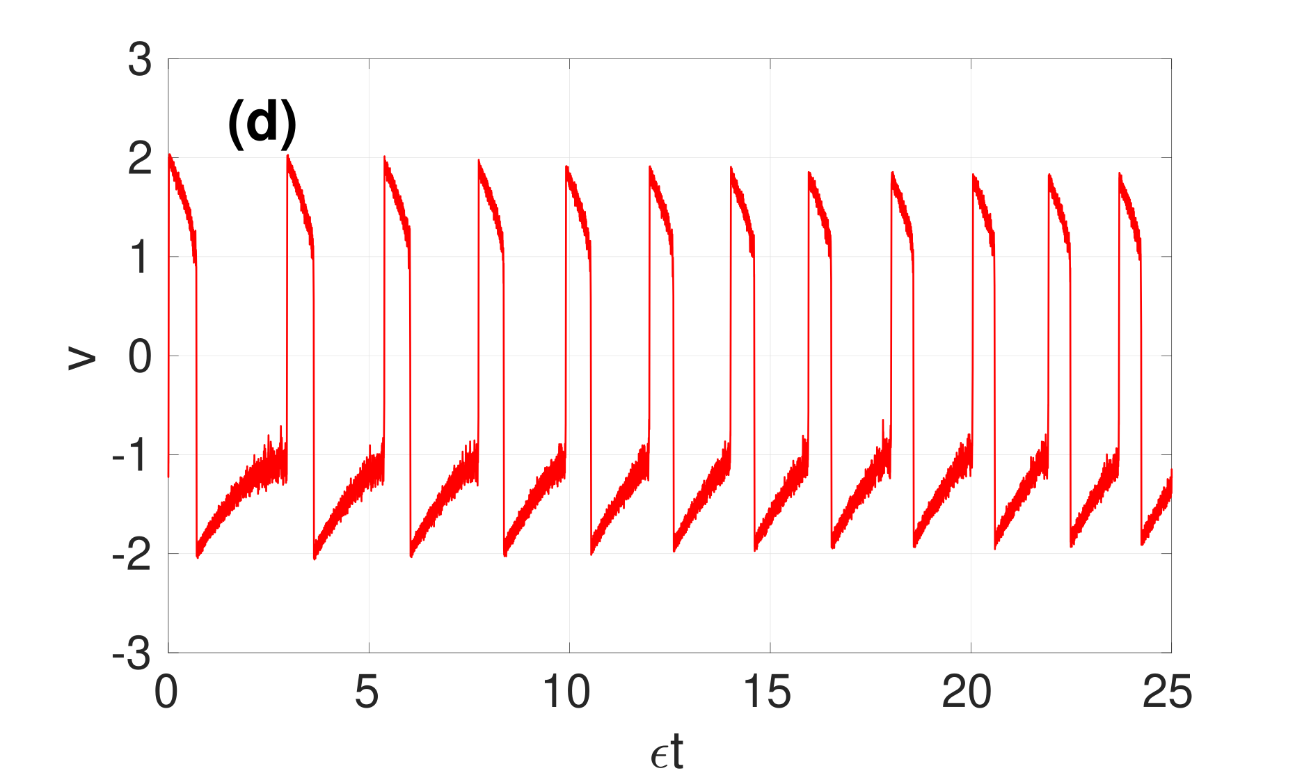
Figure 5: The variation of $CV$ with the noise intensity $\sigma$ with Lévy noise $(\alpha=0.1$, $\beta=0.0)$ in (a) and Gaussian noise $(\alpha=2.0$, $\beta=0.0)$ in (b). Time series during SISR induced by the Lévy noise in (c) with $\sigma=0.04$ and Gaussian noise in (d) with $\sigma=0.04$. Degree of SISR is higher with Lévy noise than with Gaussian noise for all values of $\sigma$. $k_{1}=0.1$ and $k_{2}=0.1$.

Fig. 6(a) and (b) show minimum coefficient of variation ($CV_{min}$) against the stability index ($\alpha$) and the skewness ($\beta$) parameters of the Lévy process in a weak ($k_{1}=0.1$ and $k_{2}=0.1$) and in a strong ($k_{1}=2.0$ and $k_{2}=1.0$) magnetic flux regime, respectively.

In Fig. 6(a), with a weak magnetic flux regime ($k_{1}=0.1$, $k_{2}=0.1$), a right-skewed (i.e., $\beta\in(0.0,1.0]$) Lévy process with a low stability index (i.e., $\alpha\in(0.0,0.7]$) can induce a high degree of SISR, as indicated by the very low value of $CV_{min}\approx 0.0014$. With higher values of $\alpha$, i.e., for $\alpha\in(1.0,2.0)$ and irrespective of the value of the skewness parameter, i.e., for $\beta\in[-1.0,1.0]$, the degree of SISR is high and almost constant as indicated by the low and almost constant $CV_{min}\approx 0.005$. Even though this cannot be clearly seen from the panel, the data shows that, at $\alpha=2.0$ and $\beta\in[-1.0,1.0]$ (which includes the Gaussian case at $\beta=0.0$), the $CV_{min}$ is also the low and almost constant at $CV_{min}\approx 0.0497$, i.e, almost 10 order of magnitude higher than the $CV_{min}$ of the Lévy processes in which $\alpha\in(1.0,2)$ and $\beta\in[-1.0,1.0]$. And for $\alpha\in(0.0,1.0]$ and $\beta\in[-1.0,-0.5]$ (i.e., from the bright red, the yellow, and the white regions), the degree of SISR is relatively low, as $CV_{min}$ continuously vary in the interval $CV_{min}\in[0.125,0.328]$ with the highest value at $CV_{min}\approx 0.328$, occurring at $\alpha=0.8$ and $\beta=-1.0$.

In Fig. 6(b), with a strong magnetic flux regime ($k_{1}=2.0$, $k_{2}=1.0$), the variation in the degree of SISR is qualitatively the same as in Fig. 6(a), but data show that there is a slight quantitative difference in the oder of magnitude of the $CV_{min}$ values, and hence in the degree of SISR in both panels. For example, when we have Gaussian noise (i.e., $\alpha=2.0$ and $\beta=0.0$), we have a $CV_{min}\approx 0.0538$ for weak magnetic flux in Fig. 6(a) and $CV_{min}\approx 0.0497$ for strong magnetic flux in Fig. 6(b). Later, we shall discuss and show more clearly in the $(k_{1},k_{2})$-plane the effects of the magnetic gain parameters on the degree of SISR.

The presence of intermittent intervals of sub-threshold spiking explains the relatively high values of $CV_{min}\in[0.125,0.328]$ in the region bounded by $\alpha\in(0.0,1.0]$ and $\beta\in[-1.0,-0.5]$ (i.e., the bright red, yellow, and white regions) in the panels of Fig. 6. Because of these intervals of intermittent sub-threshold spiking (with $v\leq v_{th}=1.3$, an arbitrarily chosen threshold value), the regularity of the ISIs which is calculated based on the occurrence of supra-threshold spiking (with $v>v_{th}$) is deteriorated. On the other hand, for parameter values in the regions bounded by $\alpha\in(0.0,1.0]$ and $\beta\in(-0.5,1.0]$ (i.e., dark region with $CV_{min}\approx 0.0014$), $\alpha\in(1.0,2.0)$ and $\beta\in[-1.0,1.0]$ (i.e., dark region with $CV_{min}\approx 0.005$), and by $\alpha=2.0$ and $\beta\in[-1.0,1.0]$ (i.e., dark region with $CV_{min}\approx 0.0497$), the time series contain fewer intermittent intervals of sub-threshold spiking (see, e.g., Fig. 5(c)), hence the low value of the $CV_{min}$ in these regions.

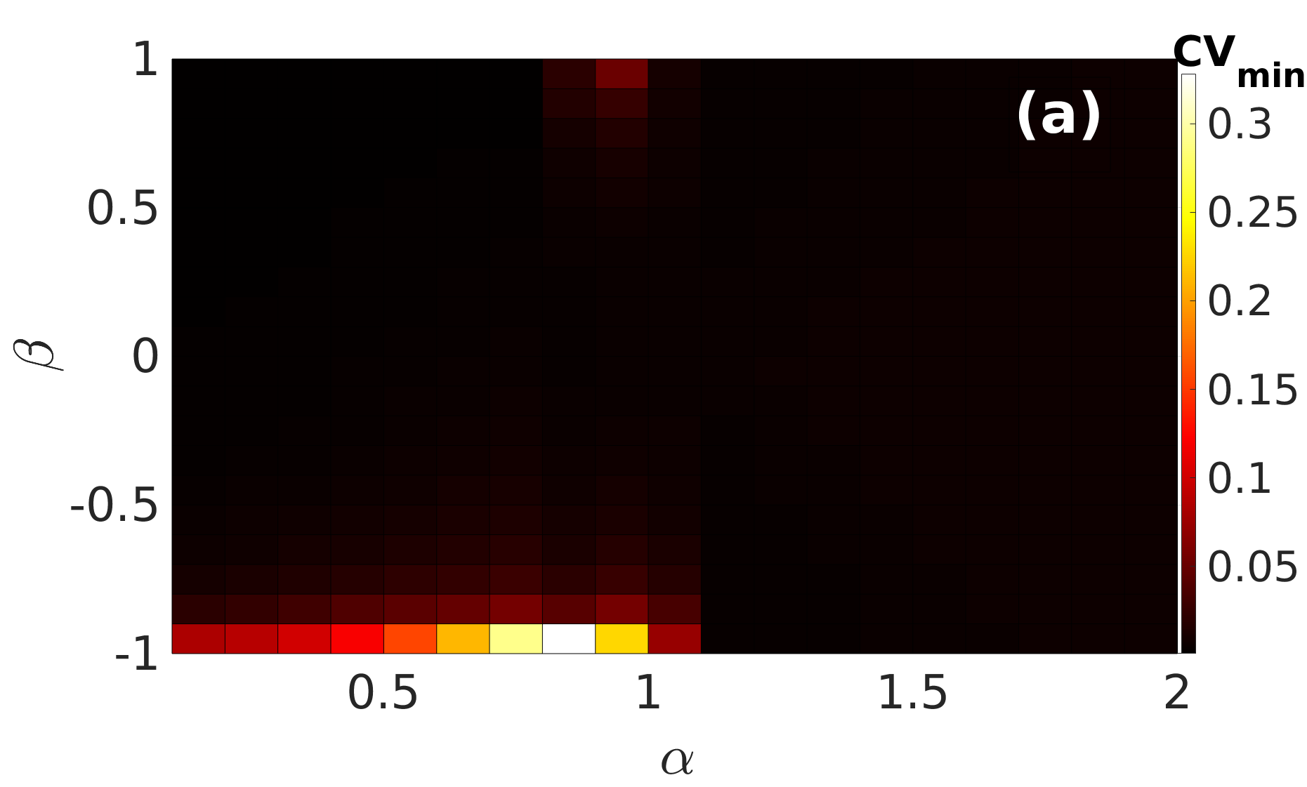
Figure 6: Variations of the minimum CV ($CV_{min}$) with respect to the stability index ($\alpha$) and the skewness ($\beta$) parameters with weak ($k_{1}=0.1$, $k_{2}=0.1$) and strong ($k_{1}=2.0$, $k_{2}=1.0$) magnetic gain parameters in (a) and (b), respectively.

In Fig. 7, we show the variation in the degree of SISR with the variations in the strengths of the magnetic gain parameters $k_{1}$ and $k_{2}$ in three specific regions of interest in Fig. 6(a): (i) when the degree of SISR is low, i.e., in the white spot with $\alpha=0.7$ and $\beta=-1.0$, (ii) when the degree of SISR is high, i.e., the dark red region with $\alpha=2.0$ and $\beta=0.0$ (i.e., Gaussian), and (iii) when the degree of SISR is very high, i.e., the black region with $\alpha=0.1$ and $\beta=1.0$. We also note that in all the panels of Fig. 7, the magnetic gain parameter $k_{2}$ is restricted to $k_{2}\geq 1.0$, so that the memristive neuron always lies in the excitability region (black region) for all values of $k_{1}\geq 0.0$, as indicated in Fig. 2(b).

In Fig. 7(a), we can now clearly see the effects of the magnetic gain parameters on the degree of SISR when $\alpha=0.7$ and $\beta=-1.0$, corresponding, from Fig. 6(a), to the white spot with a relatively large $CV_{min}\approx 0.328$. We observe that: the stronger the magnetic gain parameter $k_{1}$ — that bridges the coupling and modulation on the membrane potential $v$ from magnetic field $\phi$ — and the weaker the parameter $k_{2}$ — that describes the degree of polarization and magnetization by adjusting the saturation of magnetic flux — the higher the degree of SISR. In Fig. 7(a), as $k_{1}\rightarrow 2.0$ and $k_{2}\rightarrow 1.0$, the color-coded $CV_{min}$ goes from a white region with a relatively high value of $CV_{min}\approx 0.69$, via a yellow and a red, to a black region with the lowest $CV_{min}\approx 0.30$. Moreover, irrespective of the value of $k_{2}$, when $k_{1}=0.0$, $CV_{min}$ takes the highest value of the panel (i.e., $CV_{min}\approx 0.69$ in the white region). Further numerical simulations (not shown) indicated that this behavior is qualitatively the same for many pairs of values of $\alpha\in(0.0,1.0]$ and $\beta\in[-1.0,-0.5]$. This means that the appropriate combination of values of the magnetic gain parameters can significantly improve the degree of SISR induced by Lévy noise when the noise parameters are in intervals $\alpha\in[0.0,1.0]$ and $\beta\in[-1.0,-0.5]$. We shall see later in Fig. 7(c) that this significant improvement in the degree of SISR depends on intervals in which $\alpha$ and $\beta$ are located.

In Fig. 7(b), we have Gaussian noise (i.e., $\alpha=2.0$ and $\beta=0.0$) and effects of the magnetic gain parameters are qualitatively the same as in Fig. 7(a) with a Lévy noise having parameters at $\alpha=0.7$ and $\beta=-1.0$. That is, the weaker $k_{2}$ and the stronger $k_{1}$ become, the lower is $CV_{min}$, on average.

It is worth noting, by comparing Fig. 7(a) and (b), that the degree of SISR induced by Lévy noise (with $\alpha=0.7$ and $\beta=-1.0$) is lower than that induced by Gaussian noise ($\alpha=2.0$ and $\beta=0.0$). Furthermore, the effects of the magnetic gain parameters $k_{1}$ and $k_{2}$ on the degree of SISR is weaker in the Gaussian case. That is, in Fig. 7(b), $CV_{min}$ varies in the interval $[0.044,0.121]$, compared to $[0.30,0.69]$ in Fig. 7(a). The bigger range in the latter interval indicates the stronger effects of the magnetic gain parameters on the degree of SISR induced by Lévy noise when its parameters lie in the intervals $\alpha\in(0.0,1.0]$ and $\beta\in[-1.0,-0.5]$.

Moreover, it important to note that the degree of SISR in the non-memristive neuron (i.e., when $k_{1}=0$) is always lower (poorer) than that in the memristive one. This result is confirmed by comparing $CV_{min}$ in the non-memristive FHN neuron perturbed by Gaussian noise — studied in our previous work [90] — to the memristive FHN model studied in the current paper. In the non-memristive case, the lowest $CV$ value is always at $CV\approx 0.2$, while in the memristive case, the lowest value gets even smaller, i.e., $CV\approx 0.044$, especially as $k_{1}\to 2$ and $k_{2}\to 1$.

In Fig. 7(c), we have a Lévy noise with $\alpha=0.1$ and $\beta=1.0$, which corresponds to a black region (i.e., with a high degree of SISR) in Fig. 6(a). In this case, just as in Fig. 7(a), as $k_{1}\to 2$ and $k_{2}\to 1$, the higher the degree of SISR. However, the magnetic gain parameters ($k_{1}$ and $k_{2}$) have weaker effects on the high degree of SISR compared to when the Lévy process is very impulsive, as for example, in Fig. 7(a). In Fig. 7(c), the degree of SISR remains very high with a $CV_{min}$ varying within an extremely thin interval of $[0.000789,0.000804]$, for all values of $k_{1}$ and $k_{2}$. In this case, the Lévy process with $\alpha=0.1$ and $\beta=1.0$ induces a higher degree of SISR than the Gaussian process, in contrast to a Lévy process with $\alpha=0.7$ and $\beta=-1.0$.

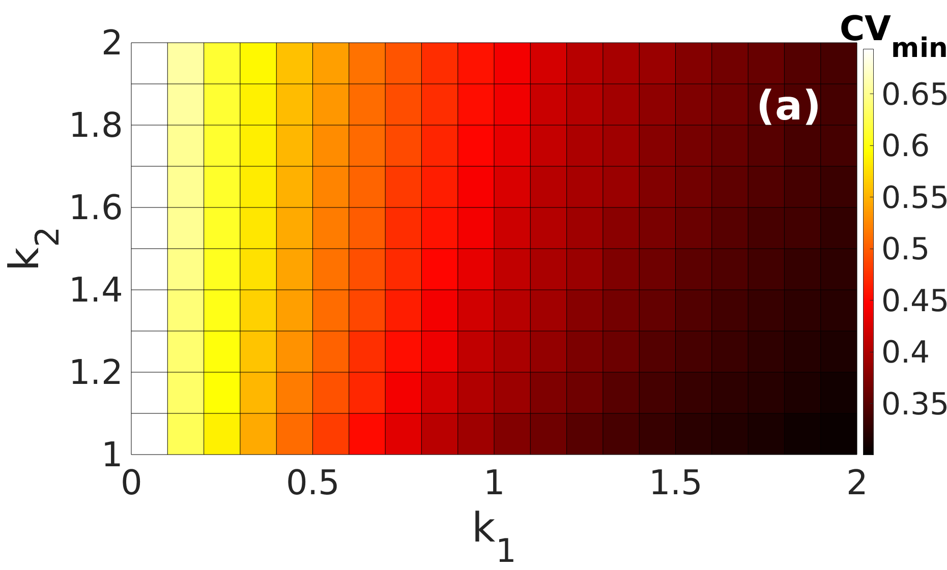
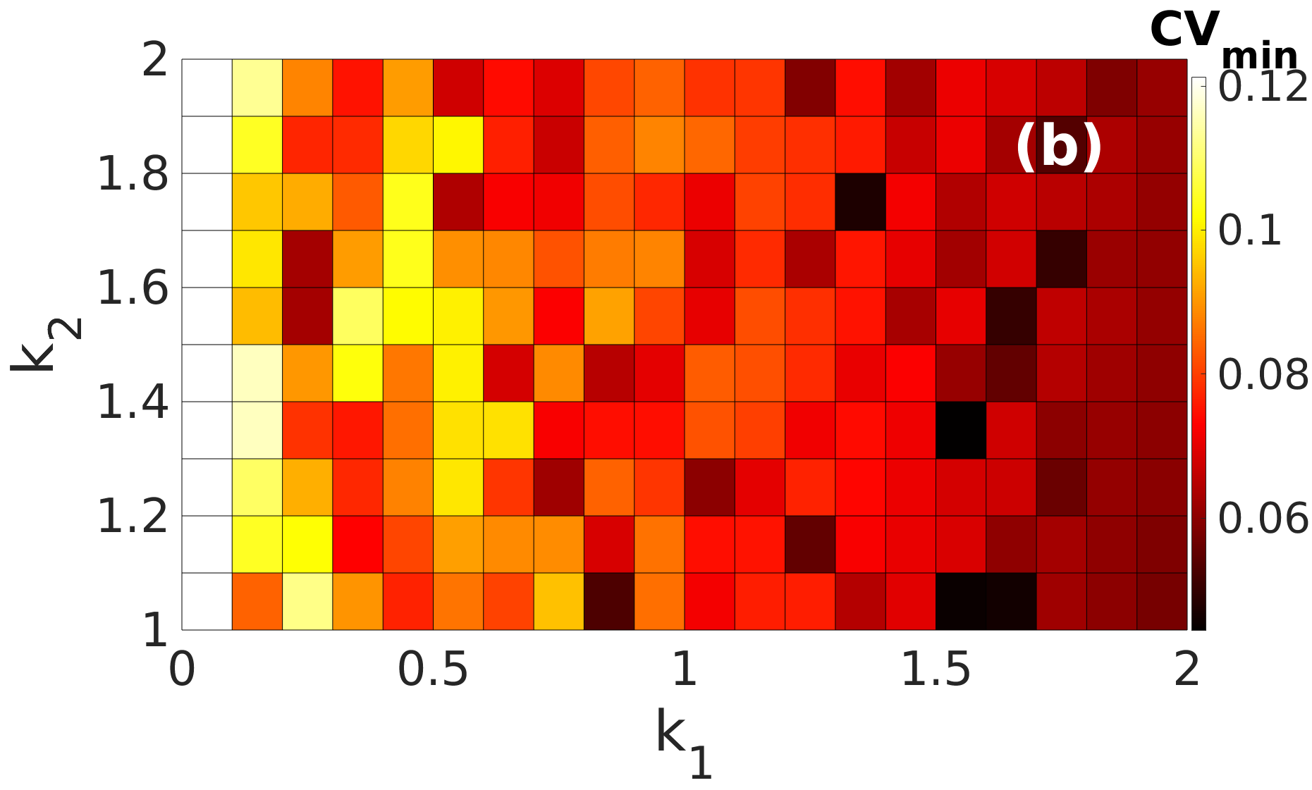
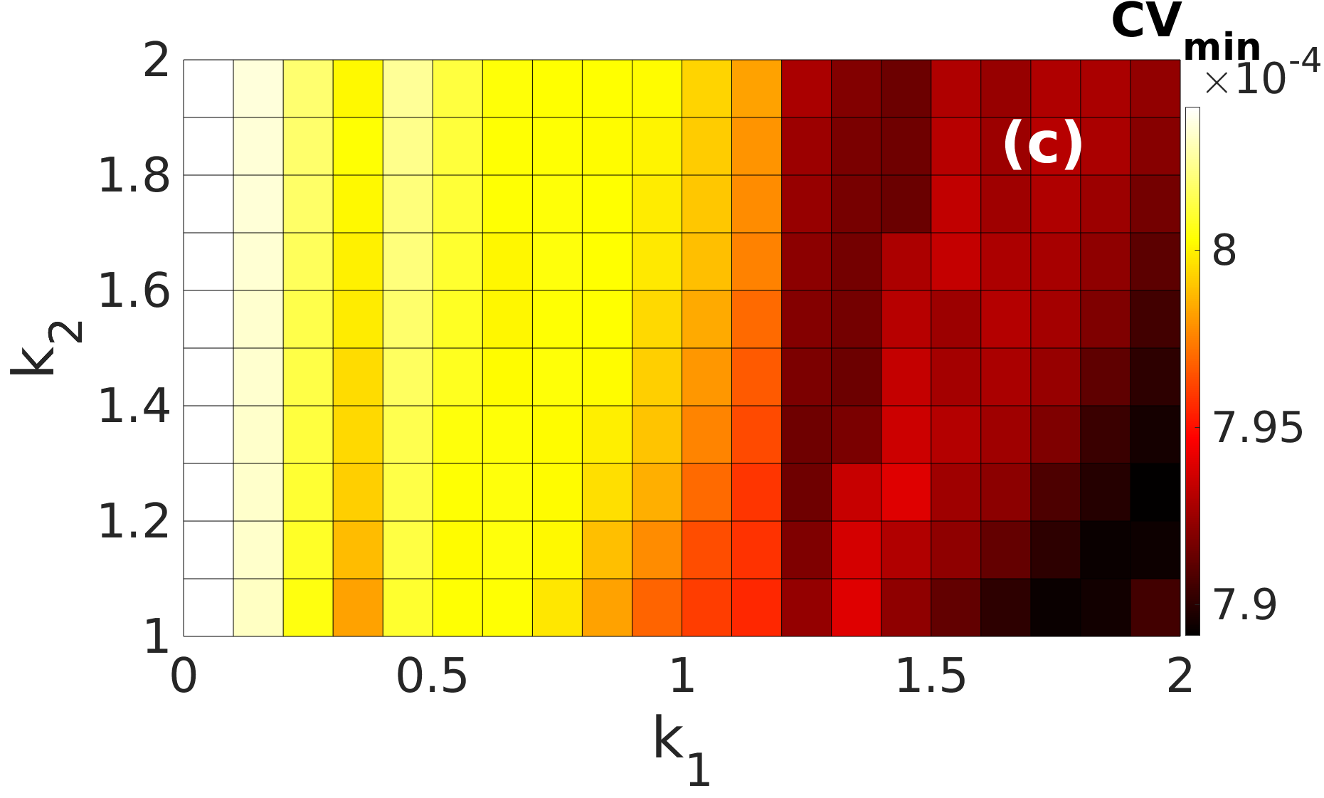
Figure 7: Variations of the minimum CV ($CV_{min}$) with respect to the magnetic gain parameters $k_{1}$ and $k_{2}$ at different values of the stability index and skewness parameters. In all cases, the larger $k_{1}$ is and the smaller $k_{2}$ is, the lower is the value of $CV_{min}$, i.e., the higher the degree of SISR. In (a): $\alpha=0.7$, $\beta=-1.0$; in (b): $\alpha=2.0$, $\beta=0.0$; and (c): $\alpha=0.1$, $\beta=1.0$.

In the adiabatic limit $\varepsilon\to 0$, the fact that stronger magnetic flux $k_{1}$ can significantly improve the degree of SISR with a Gaussian or a Lévy process can theoretically be explained in term of the potential landscapes in Fig. 3 and the mean exit times given by Eq. (18). In the Gaussian case, mean exit times depend exponentially on the barrier functions $\bigtriangleup U_{\pm}$ (see Eq. (19)) which should not be too deep, so that weaker noise intensities can be sufficient to provoke jumps (spikes) from one potential well to another. So as $k_{1}\to 2$ (i.e., becomes stronger), $\bigtriangleup U_{\pm}\to 0$ (i.e., become shallower, see Fig. 3), and the more easily weak noise intensities can provoke frequent spikes. And if this frequent spiking is combined with the scaling limits in Eq. (24), the degree of SISR gets higher (i.e., $CV_{min}\to 0.0$).

In the Lévy cases, mean exit times in Eq. (18) depend on the location of the minima $v_{l}$ and $v_{r}$ and hence, also on band widths of the wells (i.e., the distances from the minima $v=v_{l}$ and $v=v_{r}$ of the wells to the saddle point $v=v_{m}=0.0$; see Fig. 3 which shows a reduction in the distance between the short vertical bars all located at these minima, and the point $v=0$, as $k_{1}$ increases). The shorter these band widths are (i.e., the closer $v_{l}$ and $v_{r}$ are to $v_{m}=0.0$), the shorter the mean exit times given in Eq. (18). Thus, weak noise intensities can more easily provoke frequent jumps (spikes) from one potential well to another. When this frequent spiking is combined with the scaling limits in Eq. (23), the degree of SISR gets higher.

However, when the Lévy noise becomes impulsive (i.e., as $\alpha\to 0$, with a variance that tends to infinity, see Fig. 1 and also [29]), the anomalous instantaneous long jumps of trajectories becomes significant. In this case, the band widths which are controlled by magnetic gain parameter $k_{1}$ do not longer have significant effects on the mean exit times. Thus, as $\alpha\to 0$, the variation in the magnetic gain parameters should also not have too much effects on the high degree of SISR as long as Eq. (23) is satisfied. This is what we observe in Fig. 7(c) with $\alpha=0.1$ and $\beta=1.0$.

Nevertheless, this inability to significantly change the degree of SISR when $\alpha\in(0.0,1.0]$, depends also on the skewness of the Lévy noise. If the noise is left-skewed (as e.g., in Fig. 7(a) with, in particular $\beta=-1.0$), then the left potential well (i.e., the left stable branch of the cubic nullcline on which the unique stable fixed point is located) is favoured compared to the right well (i.e., the right stable branch). This results into trajectories staying a bit longer in this left well, provoking these intermittent intervals of sub-threshold spiking which destroys the regularity of the ISIs. In this left-skewed case, the magnetic gain parameters have significant effect on the degree of SISR as we saw in Fig. 7(a).

5 Summary and conclusions

In this paper, we investigated and compared the mechanism of SISR induced by Lévy white noise and Gaussian white noise in a memristive FHN neuron. We showed that depending on the parameter values ($\alpha\in(0,2)$ and $\beta\in[-1,1]$) of the Lévy noise, the neuron could exhibit a very high degree of SISR with a minimum coefficient of variation as low as 0.000789, compared to 0.044 in the case of Gaussian noise. However, the degree of SISR induced by a Lévy noise is not always higher than that induced by the Gaussian noise. In particular, in the intervals $\alpha\in(0.0,1.0]$ and $\beta\in[-1.0,-0.5]$, the Lévy processes induce a lower degree of SISR (with $CV_{min}\in[0.125,0.328]$) than the Gaussian process with $CV_{min}\approx 0.0497$.

It is shown that, the stronger magnetic gain parameter $k_{1}$ (i.e., the parameter that bridges the coupling and modulation on membrane potential $v$ from magnetic field $\phi$) and the weaker $k_{2}$ (i.e., the parameter that controls the degree of polarization and magnetization by adjusting the saturation of magnetic field $\phi$) are, the higher the degree of SISR for both Lévy and Gaussian processes. However, in the Lévy case, this combined effect of the magnetic gain parameters on the degree of SISR becomes less significant when the process becomes more impulsive (i.e., as $\alpha\to 0$) and right-skewed (with $\beta\to 1$). Moreover, it has been shown, for both types of noises, that the degree of SISR in the memristive neuron (i.e., when $k_{1}\neq 0$ and $k_{2}\neq 0$) is always higher than the degree in the non-memristive neuron (i.e., when $k_{1}=0$ and $k_{2}=0$).

Looking forward, we must be cognizant that Lévy white noise is only one possible type of a non-Gaussian white noise which can induce SISR. The mechanism via which noise with a temporal correlation (i.e., colored noise) can induce SISR is worth investigating. The additional timescale brought into the system by this temporal correlation may come along with new interesting dynamics.

References

- Bao et al. [2010] Bao, B., Liu, Z., Xu, J., 2010. Steady periodic memristor oscillator with transient chaotic behaviours. Electronics letters 46, 237–238.
- Barndorff-Nielsen and Shephard [2001] Barndorff-Nielsen, O.E., Shephard, N., 2001. Non-gaussian ornstein–uhlenbeck-based models and some of their uses in financial economics. Journal of the Royal Statistical Society: Series B (Statistical Methodology) 63, 167–241.
- Bertoin [1996] Bertoin, J., 1996. Lévy processes cambridge university press. Melbourne, NY .
- Burrage et al. [2006] Burrage, K., Burrage, P., Higham, D.J., Kloeden, P.E., Platen, E., 2006. Comment on “Numerical methods for stochastic differential equations”. Phys. Rev. E 74, 068701.
- Carrillo et al. [2004] Carrillo, O., Santos, M.A., García-Ojalvo, J., Sancho, J., 2004. Spatial coherence resonance near pattern-forming instabilities. EPL (Europhysics Letters) 65, 452.
- Chechkin et al. [2007] Chechkin, A.V., Sliusarenko, O.Y., Metzler, R., Klafter, J., 2007. Barrier crossing driven by Lévy noise: Universality and the role of noise intensity. Phys. Rev. E 75, 041101.
- Chua [1971] Chua, L., 1971. Memristor-the missing circuit element. IEEE Transactions on circuit theory 18, 507–519.
- Collins et al. [1996] Collins, J.J., Imhoff, T.T., Grigg, P., 1996. Noise-enhanced information transmission in rat sa1 cutaneous mechanoreceptors via aperiodic stochastic resonance. Journal of Neurophysiology 76, 642–645.
- DeVille and Vanden-Eijnden [2007] DeVille, R.L., Vanden-Eijnden, E., 2007. A nontrivial scaling limit for multiscale markov chains. Journal of Statistical Physics 126, 75–94.
- DeVille et al. [2005] DeVille, R.L., Vanden-Eijnden, E., Muratov, C.B., 2005. Two distinct mechanisms of coherence in randomly perturbed dynamical systems. Physical Review E 72, 031105.
- DeVille et al. [2007] DeVille, R.L., Vanden-Eijnden, E., et al., 2007. Self-induced stochastic resonance for brownian ratchets under load. Communications in Mathematical Sciences 5, 431–466.
- Ditlevsen [1999] Ditlevsen, P.D., 1999. Anomalous jumping in a double-well potential. Physical Review E 60, 172.
- Douglass et al. [1993] Douglass, J.K., Wilkens, L., Pantazelou, E., Moss, F., 1993. Noise enhancement of information transfer in crayfish mechanoreceptors by stochastic resonance. Nature 365, 337–340.
- Dubkov et al. [2008] Dubkov, A.A., Spagnolo, B., Uchaikin, V.V., 2008. Lévy flight superdiffusion: an introduction. International Journal of Bifurcation and Chaos 18, 2649–2672.
- Dybiec and Gudowska-Nowak [2009] Dybiec, B., Gudowska-Nowak, E., 2009. Lévy stable noise-induced transitions: stochastic resonance, resonant activation and dynamic hysteresis. Journal of Statistical Mechanics: Theory and Experiment 2009, P05004.
- Dybiec et al. [2016] Dybiec, B., Gudowska-Nowak, E., Chechkin, A., 2016. To hit or to pass it over—remarkable transient behavior of first arrivals and passages for lévy flights in finite domains. Journal of Physics A: Mathematical and Theoretical 49, 504001.
- Dybiec et al. [2007] Dybiec, B., Gudowska-Nowak, E., Hänggi, P., 2007. Escape driven by -stable white noises. Physical Review E 75, 021109.
- Feng et al. [2019] Feng, J., Xu, W., Xu, Y., Wang, X., 2019. Effects of lévy noise in a neuronal competition model. Physica A: Statistical Mechanics and its Applications 531, 121747.
- FitzHugh [1969] FitzHugh, R., 1969. Mathematical models of excitation and propagation in nerve. Biological engineering , 1–85.
- Gammaitoni et al. [1998] Gammaitoni, L., Hänggi, P., Jung, P., Marchesoni, F., 1998. Stochastic resonance. Reviews of modern physics 70, 223.
- Górska and Penson [2011] Górska, K., Penson, K., 2011. Lévy stable two-sided distributions: Exact and explicit densities for asymmetric case. Physical Review E 83, 061125.
- Guo et al. [2018] Guo, D., Perc, M., Liu, T., Yao, D., 2018. Functional importance of noise in neuronal information processing. EPL (Europhysics Letters) 124, 50001.
- Guo et al. [2017] Guo, D., Perc, M., Zhang, Y., Xu, P., Yao, D., 2017. Frequency-difference-dependent stochastic resonance in neural systems. Physical Review E 96, 022415.
- Guo et al. [2021] Guo, Y., Wang, L., Dong, Q., Lou, X., 2021. Dynamical complexity of fitzhugh–nagumo neuron model driven by lévy noise and gaussian white noise. Mathematics and Computers in Simulation 181, 430–443.
- Gutkin et al. [2007] Gutkin, B., Jost, J., Tuckwell, H., 2007. Transient termination of spiking by noise in coupled neurons. EPL (Europhysics Letters) 81, 20005.
- Gutkin et al. [2009] Gutkin, B.S., Jost, J., Tuckwell, H.C., 2009. Inhibition of rhythmic neural spiking by noise: the occurrence of a minimum in activity with increasing noise. Naturwissenschaften 96, 1091–1097.
- Hong et al. [2013] Hong, Q.H., Zeng, Y.C., Li, Z.J., 2013. Design and simulation of chaotic circuit for flux-controlled memristor and charge-controlled memristor. Acta Physica Sinica 62.
- Huang et al. [2011] Huang, J., Tao, W., Xu, B., 2011. Effects of small time delay on a bistable system subject to lévy stable noise. Journal of Physics A: Mathematical and Theoretical 44, 385101.
- Imkeller and Pavlyukevich [2006] Imkeller, P., Pavlyukevich, I., 2006. Lévy flights: transitions and meta-stability. Journal of Physics A: Mathematical and General 39, L237–L246.
- Izhikevich [2000] Izhikevich, E.M., 2000. Neural excitability, spiking and bursting. International Journal of Bifurcation and Chaos 10, 1171–1266.
- Janicki and Weron [1993] Janicki, A., Weron, A., 1993. Simulation and chaotic behavior of alpha-stable stochastic processes. volume 178. CRC Press.
- Koren et al. [2007] Koren, T., Lomholt, M.A., Chechkin, A.V., Klafter, J., Metzler, R., 2007. Leapover lengths and first passage time statistics for lévy flights. Physical review letters 99, 160602.
- Kosko and Mitaim [2001] Kosko, B., Mitaim, S., 2001. Robust stochastic resonance: Signal detection and adaptation in impulsive noise. Physical review E 64, 051110.
- Kramers [1940] Kramers, H.A., 1940. Brownian motion in a field of force and the diffusion model of chemical reactions. Physica 7, 284–304.
- Krauss et al. [2019] Krauss, P., Prebeck, K., Schilling, A., Metzner, C., 2019. Recurrence resonance” in three-neuron motifs. Frontiers in computational neuroscience 13.
- Kuehn [2015] Kuehn, C., 2015. Multiple Time Scale Dynamics. Springer, Berlin.
- Kurrer and Schulten [1995] Kurrer, C., Schulten, K., 1995. Noise-induced synchronous neuronal oscillations. Physical Review E 51, 6213.
- Li et al. [2015] Li, Q., Zeng, H., Li, J., 2015. Hyperchaos in a 4d memristive circuit with infinitely many stable equilibria. Nonlinear Dynamics 79, 2295–2308.
- Li and Ning [2015] Li, X., Ning, L., 2015. Stochastic resonance in fizhugh-nagumo model driven by multiplicative signal and non-gaussian noise. Indian Journal of Physics 89, 189–194.
- Lindner et al. [2004] Lindner, B., Garcıa-Ojalvo, J., Neiman, A., Schimansky-Geier, L., 2004. Effects of noise in excitable systems. Physics reports 392, 321–424.
- Lisowski et al. [2015] Lisowski, B., Valenti, D., Spagnolo, B., Bier, M., Gudowska-Nowak, E., 2015. Stepping molecular motor amid lévy white noise. Physical Review E 91, 042713.
- Liu and Kang [2018] Liu, R.N., Kang, Y.M., 2018. Stochastic resonance in underdamped periodic potential systems with alpha stable lévy noise. Physics Letters A 382, 1656–1664.
- Longtin [1993] Longtin, A., 1993. Stochastic resonance in neuron models. Journal of statistical physics 70, 309–327.
- Lv et al. [2016] Lv, M., Wang, C., Ren, G., Ma, J., Song, X., 2016. Model of electrical activity in a neuron under magnetic flow effect. Nonlinear Dynamics 85, 1479–1490.
- M. E. Yamakou [2020] M. E. Yamakou, 2020. Chaotic synchronization of memristive neurons: Lyapunov function versus Hamilton function. Nonlinear Dynamics 101, 487–500.
- Ma et al. [2017a] Ma, J., Mi, L., Zhou, P., Xu, Y., Hayat, T., 2017a. Phase synchronization between two neurons induced by coupling of electromagnetic field. Applied Mathematics and Computation 307, 321–328.
- Ma et al. [2017b] Ma, J., Wang, Y., Wang, C., Xu, Y., Ren, G., 2017b. Mode selection in electrical activities of myocardial cell exposed to electromagnetic radiation. Chaos, Solitons & Fractals 99, 219–225.
- Ma et al. [2017c] Ma, J., Wu, F., Hayat, T., Zhou, P., Tang, J., 2017c. Electromagnetic induction and radiation-induced abnormality of wave propagation in excitable media. Physica A: Statistical Mechanics and its Applications 486, 508–516.
- Mantegna and Stanley [1995] Mantegna, R.N., Stanley, H.E., 1995. Scaling behaviour in the dynamics of an economic index. Nature 376, 46–49.
- Mitaim and Kosko [2004] Mitaim, S., Kosko, B., 2004. Adaptive stochastic resonance in noisy neurons based on mutual information. IEEE transactions on neural networks 15, 1526–1540.
- Muratov and Vanden-Eijnden [2008] Muratov, C.B., Vanden-Eijnden, E., 2008. Noise-induced mixed-mode oscillations in a relaxation oscillator near the onset of a limit cycle. Chaos: An Interdisciplinary Journal of Nonlinear Science 18, 015111.
- Muratov et al. [2005] Muratov, C.B., Vanden-Eijnden, E., Weinan, E., 2005. Self-induced stochastic resonance in excitable systems. Physica D: Nonlinear Phenomena 210, 227–240.
- Muthuswamy [2010] Muthuswamy, B., 2010. Implementing memristor based chaotic circuits. International Journal of Bifurcation and Chaos 20, 1335–1350.
- Neiman et al. [1997] Neiman, A., Saparin, P.I., Stone, L., 1997. Coherence resonance at noisy precursors of bifurcations in nonlinear dynamical systems. Physical Review E 56, 270.
- Novikov et al. [2005] Novikov, D.S., Drndic, M., Levitov, L., Kastner, M., Jarosz, M., Bawendi, M., 2005. Lévy statistics and anomalous transport in quantum-dot arrays. Physical Review B 72, 075309.
- Nozaki et al. [1999] Nozaki, D., Mar, D.J., Grigg, P., Collins, J.J., 1999. Effects of colored noise on stochastic resonance in sensory neurons. Physical Review Letters 82, 2402.
- Nurzaman et al. [2011] Nurzaman, S.G., Matsumoto, Y., Nakamura, Y., Shirai, K., Koizumi, S., Ishiguro, H., 2011. From lévy to brownian: a computational model based on biological fluctuation. PloS one 6, e16168.
- Patel and Kosko [2008] Patel, A., Kosko, B., 2008. Stochastic resonance in continuous and spiking neuron models with levy noise. IEEE Transactions on Neural Networks 19, 1993–2008.
- Pei et al. [1996] Pei, X., Wilkens, L., Moss, F., 1996. Noise-mediated spike timing precision from aperiodic stimuli in an array of hodgekin-huxley-type neurons. Physical review letters 77, 4679.
- Peng et al. [1993] Peng, C.K., Mietus, J., Hausdorff, J., Havlin, S., Stanley, H.E., Goldberger, A.L., 1993. Long-range anticorrelations and non-gaussian behavior of the heartbeat. Physical review letters 70, 1343.
- Penson and Górska [2010] Penson, K., Górska, K., 2010. Exact and explicit probability densities for one-sided lévy stable distributions. Physical review letters 105, 210604.
- Perc [2005] Perc, M., 2005. Spatial coherence resonance in excitable media. Physical Review E 72, 016207.
- Perc [2007] Perc, M., 2007. Transition from gaussian to levy distributions of stochastic payoff variations in the spatial prisoner’s dilemma game. Physical Review E 75, 022101.
- Pikovsky and Kurths [1997] Pikovsky, A.S., Kurths, J., 1997. Coherence resonance in a noise-driven excitable system. Physical Review Letters 78, 775.
- Prokhorov [1965] Prokhorov, Y.V., 1965. W. feller, an introduction to probability theory and its applications. Teoriya Veroyatnostei i ee Primeneniya 10, 204–206.
- Rocha et al. [2020] Rocha, E.G., Santos, E.P., dos Santos, B.J., Samuel, S., Pincheira, P.I., Argolo, C., Moura, A.L., 2020. Lévy flights for light in ordered lasers. Physical Review A 101, 023820.
- Rümelin [1982] Rümelin, W., 1982. Numerical treatment of stochastic differential equations. SIAM Journal on Numerical Analysis 19, 604–613.
- Sato et al. [1999] Sato, K.i., Ken-Iti, S., Katok, A., 1999. Lévy processes and infinitely divisible distributions. Cambridge university press.
- Segev et al. [2002] Segev, R., Benveniste, M., Hulata, E., Cohen, N., Palevski, A., Kapon, E., Shapira, Y., Ben-Jacob, E., 2002. Long term behavior of lithographically prepared in vitro neuronal networks. Physical review letters 88, 118102.
- Semenova and Zakharova [2018] Semenova, N., Zakharova, A., 2018. Weak multiplexing induces coherence resonance. Chaos: An Interdisciplinary Journal of Nonlinear Science 28, 051104.
- Shen et al. [2010] Shen, J., Chen, L., Aihara, K., 2010. Self-induced stochastic resonance in microrna regulation of a cancer network, in: The fourth international conference on computational systems biology, pp. 251–257.
- Shlesinger et al. [1993] Shlesinger, M.F., Zaslavsky, G.M., Klafter, J., 1993. Strange kinetics. Nature 363, 31–37.
- Stambaugh and Chan [2006] Stambaugh, C., Chan, H.B., 2006. Noise-activated switching in a driven nonlinear micromechanical oscillator. Physical Review B 73, 172302.
- Stanley and Mantegna [2000] Stanley, H.E., Mantegna, R.N., 2000. An introduction to econophysics. Cambridge University Press, Cambridge.
- Uzuntarla et al. [2013] Uzuntarla, M., Cressman, J.R., Ozer, M., Barreto, E., 2013. Dynamical structure underlying inverse stochastic resonance and its implications. Physical Review E 88, 042712.
- Wang et al. [2016] Wang, Z., Xu, Y., Yang, H., 2016. Lévy noise induced stochastic resonance in an fhn model. Science China Technological Sciences 59, 371–375.
- Weron [1996] Weron, R., 1996. On the chambers-mallows-stuck method for simulating skewed stable random variables. Statistics & probability letters 28, 165–171.
- Wiesenfeld and Moss [1995] Wiesenfeld, K., Moss, F., 1995. Stochastic resonance and the benefits of noise: from ice ages to crayfish and squids. Nature 373, 33–36.
- Wilkie [2004] Wilkie, J., 2004. Numerical methods for stochastic differential equations. Phys. Rev. E 70, 017701.
- Wu et al. [2019] Wu, F., Ma, J., Zhang, G., 2019. A new neuron model under electromagnetic field. Applied Mathematics and Computation 347, 590–599.
- Wu et al. [2017a] Wu, F., Wang, C., Jin, W., Ma, J., 2017a. Dynamical responses in a new neuron model subjected to electromagnetic induction and phase noise. Physica A: Statistical Mechanics and its Applications 469, 81–88.
- Wu et al. [2016] Wu, F., Wang, C., Xu, Y., Ma, J., 2016. Model of electrical activity in cardiac tissue under electromagnetic induction. Scientific reports 6, 1–12.
- Wu et al. [2017b] Wu, J., Xu, Y., Ma, J., 2017b. Lévy noise improves the electrical activity in a neuron under electromagnetic radiation. PLoS One 12, e0174330.
- Xu et al. [2014] Xu, B., Binczak, S., Jacquir, S., Pont, O., Yahia, H., 2014. Parameters analysis of fitzhugh-nagumo model for a reliable simulation, in: 2014 36th Annual International Conference of the IEEE Engineering in Medicine and Biology Society, IEEE. pp. 4334–4337.
- Xu et al. [2018] Xu, Y., Jia, Y., Ma, J., Hayat, T., Alsaedi, A., 2018. Collective responses in electrical activities of neurons under field coupling. Scientific reports 8, 1–10.
- Xu et al. [2013] Xu, Y., Li, J., Feng, J., Zhang, H., Xu, W., Duan, J., 2013. Lévy noise-induced stochastic resonance in a bistable system. The European Physical Journal B 86, 1–7.
- Xu et al. [2016] Xu, Y., Li, Y., Zhang, H., Li, X., Kurths, J., 2016. The switch in a genetic toggle system with lévy noise. Scientific reports 6, 1–11.
- Yamakou et al. [2020] Yamakou, M.E., Hjorth, P.G., Martens, E.A., 2020. Optimal self-induced stochastic resonance in multiplex neural networks: Electrical vs. chemical synapses. Frontiers in Computational Neuroscience 14, 62.
- Yamakou and Jost [2017] Yamakou, M.E., Jost, J., 2017. A simple parameter can switch between different weak-noise–induced phenomena in a simple neuron model. EPL (Europhysics Letters) 120, 18002.
- Yamakou and Jost [2018a] Yamakou, M.E., Jost, J., 2018a. Coherent neural oscillations induced by weak synaptic noise. Nonlinear Dynamics 93, 2121–2144.
- Yamakou and Jost [2018b] Yamakou, M.E., Jost, J., 2018b. Weak-noise-induced transitions with inhibition and modulation of neural oscillations. Biological cybernetics 112, 445–463.
- Yamakou and Jost [2019] Yamakou, M.E., Jost, J., 2019. Control of coherence resonance by self-induced stochastic resonance in a multiplex neural network. Physical Review E 100, 022313.
- Zhou et al. [2001] Zhou, C., Kurths, J., Hu, B., 2001. Array-enhanced coherence resonance: nontrivial effects of heterogeneity and spatial independence of noise. Physical review letters 87, 098101.
- Zhu [2020] Zhu, J., 2020. Phase sensitivity for coherence resonance oscillators. Nonlinear Dynamics 102, 2281–2293.
- Zolotarev [1983] Zolotarev, V., 1983. One dimensional stable distributions (american mathematical society, providence, ri). Russian original .